River Discharge Simulation in the High Andes of Southern Ecuador Using High-Resolution Radar Observations and Meteorological Station Data

 , , , and
Abstract
:
1. Introduction
2. Materials and Methods
2.1. Study Area
2.2. Data and Materials
2.3. Preparation of Input Data
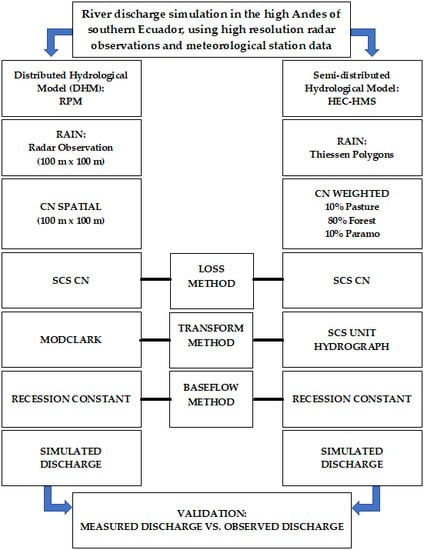
2.3.1. Distributed Hydrological Model (RPM)
2.3.2. Semi-Distributed Hydrological Model (HEC-HMS)
2.4. Validation
3. Results
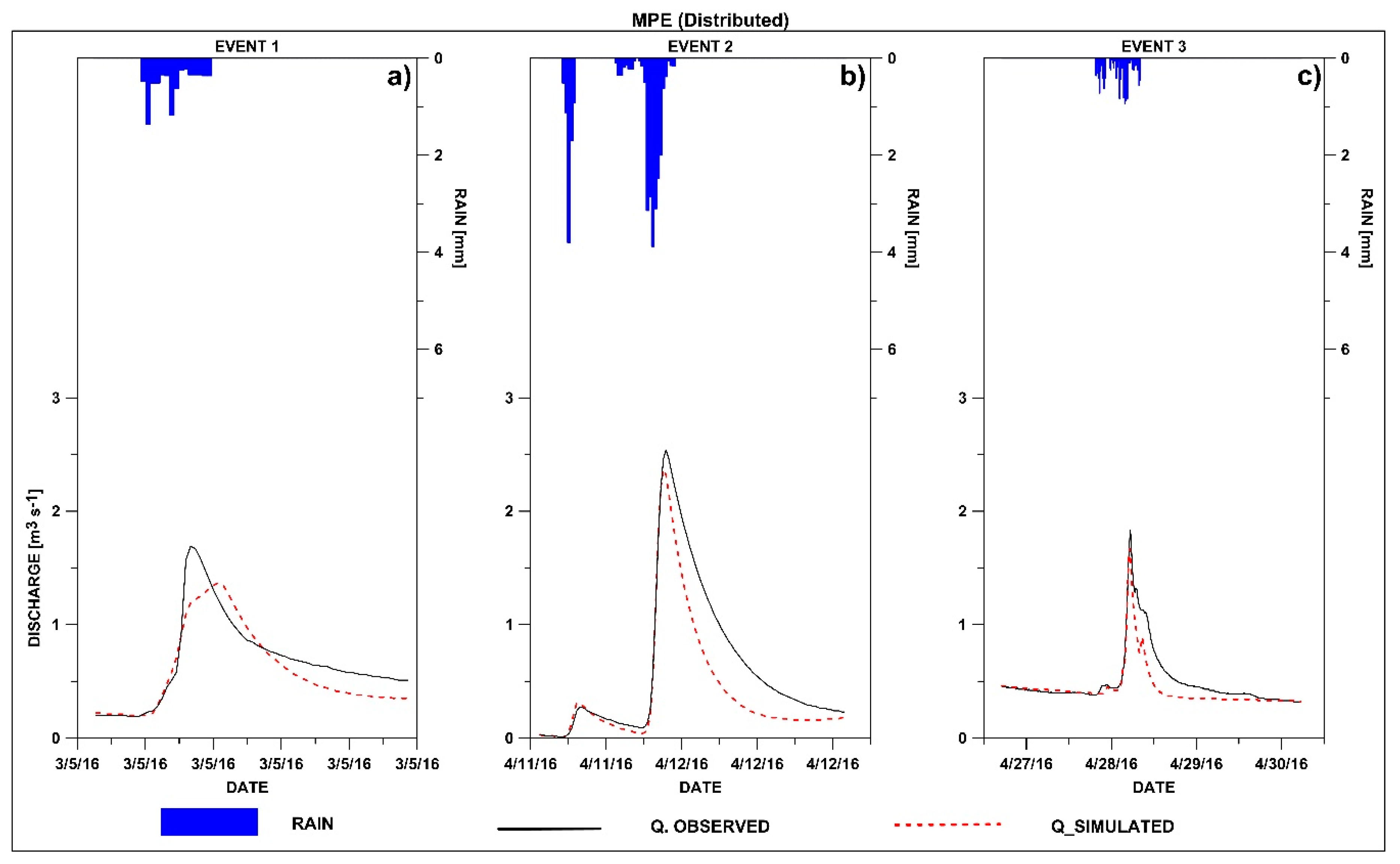
3.1. RPM Model
3.2. HEC-HMS Model
4. Discussion
5. Conclusions
Author Contributions
Funding
Acknowledgments
Conflicts of Interest
References
- Caballero, L.A.; Rimmer, A.; Easton, Z.M.; Steenhuis, T.S. Rainfall Runoff Relationships for a Cloud Forest Watershed in Central America: Implications for Water Resource Engineering. J. Am. Water Resour. Assoc. 2012, 48, 1022–1031. [Google Scholar] [CrossRef]
- Sanyal, J.; Densmore, A.L.; Carbonneau, P. Analysing the effect of land-use/cover changes at sub-catchment levels on downstream flood peaks: A semi-distributed modelling approach with sparse data. Catena 2014, 118, 28–40. [Google Scholar] [CrossRef]
- Clark, C. Storage and the Unit Hydrograph. 1945. Available online: http://ponce.sdsu.edu/clark_paper_portrait.pdf (accessed on 20 November 2019).
- Panziera, L.; Germann, U. The relation between airflow and orographic precipitation on the southern side of the Alps as revealed by weather radar. Q. J. R. Meteorolog. Soc. 2010, 136, 222–238. [Google Scholar] [CrossRef]
- Foresti, L.; Pozdnoukhov, A. Exploration of alpine orographic precipitation patterns with radar image processing and clustering techniques. Meteorol. Appl. 2012, 19, 407–419. [Google Scholar] [CrossRef]
- Coello, C.; Feyen, J.; Aguirre, L.; Morales, M. Respuesta hidrológica de microcuencas con diferente cobertura vegetal. In Proceedings of the International Congress on Development, Environment and Natural Resources: Multi-level and Multi-Scale Sustainability, Cochabamba, Bolivia, 11–13 July 2007. [Google Scholar]
- Ochoa-Cueva, P.; Fries, A.; Montesinos, P.; Rodríguez-Díaz, J.A.; Boll, J. Spatial estimation of soil erosion risk by land-cover change in the Andes of southern Ecuador. Land Degrad. Dev. 2015, 26, 565–573. [Google Scholar] [CrossRef]
- De Bièvre, B.; Acosta, L. Ecosistemas Altoandinos, Cuencas y Regulación Hídrica; CONDESAN: Quito, Ecuador, 2012. [Google Scholar]
- Wang, S.; Fu, B.-J.; He, C.-S.; Sun, G.; Gao, G.-Y. A comparative analysis of forest cover and catchment water yield relationships in northern China. For. Ecol. Manag. 2011, 262, 1189–1198. [Google Scholar] [CrossRef]
- Vázquez Zambrano, R.F. Modelación Hidrológica de Una Microcuenca Altoandina Ubicada en el Austro Ecuatoriano; Engineer-Universidad de Cuenca: Cuenca, Ecuador, 2010. [Google Scholar]
- Behrends, F.; Chagas, C.I.; Vázquez, G.; Palacín, E.A.; Santanatoglia, O.J.; Castiglioni, M.G.; Massobrio, M.J. Aplicación del Modelo Hidrológico-Swat-en una microcuenca agrícola de la Pampa Ondulada. Ciencia del suelo 2011, 29, 75–82. [Google Scholar]
- Célleri, R.; Feyen, J. The hydrology of tropical Andean ecosystems: Importance, knowledge status, and perspectives. Mt. Res. Dev. 2009, 29, 350–356. [Google Scholar] [CrossRef]
- Ciach, G.J.; Krajewski, W.F. Analysis and modeling of spatial correlation structure in small-scale rainfall in Central Oklahoma. Adv. Water Resour. 2006, 29, 1450–1463. [Google Scholar] [CrossRef]
- Tapiador, F.J.; Hou, A.Y.; De Castro, M.; Checa, R.; Cuartero, F.; Barros, A.P. Precipitation estimates for hydroelectricity. Energy Environ. Sci. 2011, 4, 4435–4448. [Google Scholar] [CrossRef]
- Refsgaard, J.C. Terminology, Modelling Protocol and Classification of Hydrological Model Codes. In Distributed Hydrological Modelling; Abbott, M.B., Refsgaard, J.C., Eds.; Springer: Dordrecht, The Netherlands, 1996; pp. 17–39. [Google Scholar]
- Jajarmizadeh, M.; Harun, S.; Salarpour, M. A Review on Theoretical Consideration and Types of Models in Hydrology. J. Environ. Sci. Technol. 2012, 5, 249–261. [Google Scholar] [CrossRef]
- Crespo, P.; Coello, C.; Iñiguez, V.; Cisneros, F.; Cisneros, P.; Ramírez, M.; Feyen, J. Evaluación de SWAT2000 Como Herramienta Para el Análisis de Escenarios de Cambio de uso del suelo en Microcuencas de Montaña del sur del Ecuador. Paper presented at the XI Congreso Ecuatoriano de la Ciencia del Suelo, Quito, Ecuador, 29–31 October 2008. [Google Scholar]
- Méndez-Antonio, B.; Soto-Cortés, G.; Rivera-Trejo, F.; Caetano, E. Modelación hidrológica distribuida apoyada en radares meteorológicos. Tecnología y ciencias del agua 2014, 5, 83–101. [Google Scholar]
- Anand, J.; Gosain, A.K.; Khosa, R.; Srinivasan, R. Regional scale hydrologic modeling for prediction of water balance, analysis of trends in streamflow and variations in streamflow: The case study of the Ganga River basin. J. Hydrol. Reg. Stud. 2018, 16, 32–53. [Google Scholar] [CrossRef]
- Plesca, I.; Timbe, E.; Exbrayat, J.-F.; Windhorst, D.; Kraft, P.; Crespo, P.; Vaché, K.B.; Frede, H.-G.; Breuer, L. Model intercomparison to explore catchment functioning: Results from a remote montane tropical rainforest. Ecol. Modell. 2012, 239, 3–13. [Google Scholar] [CrossRef]
- Behrangi, A.; Khakbaz, B.; Jaw, T.C.; AghaKouchak, A.; Hsu, K.; Sorooshian, S. Hydrologic evaluation of satellite precipitation products over a mid-size basin. J. Hydrol. 2011, 397, 225–237. [Google Scholar] [CrossRef]
- Fries, A.; Rollenbeck, R.; Bayer, F.; Gonzalez, V.; Onate-Valivieso, F.; Peters, T.; Bendix, J. Catchment precipitation processes in the San Francisco valley in southern Ecuador: Combined approach using high-resolution radar images and in situ observations. Meteorol. Atmos. Phys. 2014, 126, 13–29. [Google Scholar] [CrossRef]
- Ochoa, P.A.; Chamba, Y.M.; Arteaga, J.G.; Capa, E.D. Estimation of suitable areas for coffee growth using a GIS approach and multicriteria evaluation in regions with scarce data. Appl. Eng. Agric. 2017, 33, 841–848. [Google Scholar] [CrossRef]
- Crespo, P.; Célleri, R.; Buytaert, W.; Ochoa, B.; Cárdenas, I.; Iñiguez, V.; Borja, P.; De Bièvre, B. Impactos del cambio de uso de la tierra sobre la hidrología de los páramos húmedos andinos. In Avances en Investigación Para la Conservación de los Páramos Andinos; CONDESAN: Quito, Ecuador, 2014; pp. 288–304. [Google Scholar]
- Pedersen, L.; Jensen, N.E.; Christensen, L.E.; Madsen, H. Quantification of the spatial variability of rainfall based on a dense network of rain gauges. Atmos. Res. 2010, 95, 441–454. [Google Scholar] [CrossRef]
- Berne, A.; Krajewski, W.F. Radar for hydrology: Unfulfilled promise or unrecognized potential? Adv. Water Resour. 2013, 51, 357–366. [Google Scholar] [CrossRef]
- Chen, Y.; Liu, H.; An, J.; Görsdorf, U.; Berger, F.H. A field experiment on the small-scale variability of rainfall based on a network of micro rain radars and rain gauges. J. Appl. Meteorol. Climatol. 2015, 54, 243–255. [Google Scholar] [CrossRef]
- Morin, E.; Goodrich, D.C.; Maddox, R.A.; Gao, X.; Gupta, H.V.; Sorooshian, S. Rainfall modeling for integrating radar information into hydrological model. Atmos. Sci. Lett. 2005, 6, 23–30. [Google Scholar] [CrossRef]
- Bendix, J.; Fries, A.; Zárate, J.; Trachte, K.; Rollenbeck, R.; Pucha-Cofrep, F.; Paladines, R.; Palacios, I.; Orellana, J.; Oñate-Valdivieso, F. RadarNet-Sur first weather radar network in tropical high mountains. Bull. Am. Meteorol. Soc. 2017, 98, 1235–1254. [Google Scholar] [CrossRef]
- Oñate-Valdivieso, F.; Fries, A.; Mendoza, K.; Gonzalez-Jaramillo, V.; Pucha-Cofrep, F.; Rollenbeck, R.; Bendix, J. Temporal and spatial analysis of precipitation patterns in an Andean region of southern Ecuador using LAWR weather radar. Meteorol. Atmos. Phys. 2018, 130, 473–484. [Google Scholar] [CrossRef]
- Guerra-Cobián, V.H.; Bâ, K.M.; Quentin-Joret, E.; Díaz-Delgado, C.; Cârsteanu, A.A. Empleo de información NEXRAD en el modelado hidrológico para cuencas con pluviometría deficiente. Tecnología y ciencias del agua 2011, 2, 35–48. [Google Scholar]
- Germann, U.; Berenguer, M.; Sempere-Torres, D.; Zappa, M. REAL—Ensemble radar precipitation estimation for hydrology in a mountainous region. Q. J. R. Meteorolog. Soc. 2009, 135, 445–456. [Google Scholar] [CrossRef]
- Tridon, F.; Battaglia, A.; Watters, D. Evaporation in action sensed by multiwavelength Doppler radars. J. Geophys. Res. Atmos. 2017, 122, 9379–9390. [Google Scholar] [CrossRef]
- Orellana-Alvear, J.; Célleri, R.; Rollenbeck, R.; Bendix, J. Analysis of Rain Types and Their Z–R Relationships at Different Locations in the High Andes of Southern Ecuador. J. Appl. Meteorol. Climatol. 2017, 56, 3065–3080. [Google Scholar] [CrossRef]
- Craciun, C.; Catrina, O. An objective approach for comparing radar estimated and rain gauge measured precipitation. Meteorol. Appl. 2016, 23, 683–690. [Google Scholar] [CrossRef]
- Chu, Z.; Ma, Y.; Zhang, G.; Wang, Z.; Han, J.; Kou, L.; Li, N. Mitigating Spatial Discontinuity of Multi-Radar QPE Based on GPM/KuPR. Hydrology 2018, 5, 48. [Google Scholar] [CrossRef]
- Ośródka, K.; Szturc, J.; Jurczyk, A. Chain of data quality algorithms for 3-D single-polarization radar reflectivity (RADVOL-QC system). Meteorol. Appl. 2014, 21, 256–270. [Google Scholar] [CrossRef]
- Villarini, G.; Krajewski, W.F. Review of the different sources of uncertainty in single polarization radar-based estimates of rainfall. Surv. Geophys. 2010, 31, 107–129. [Google Scholar] [CrossRef]
- Rollenbeck, R.; Bendix, J. Rainfall distribution in the Andes of southern Ecuador derived from blending weather radar data and meteorological field observations. Atmos. Res. 2011, 99, 277–289. [Google Scholar] [CrossRef]
- Zhu, D.; Xuan, Y.; Cluckie, I. Hydrological appraisal of operational weather radar rainfall estimates in the context of different modelling structures. Hydrol. Earth Syst. Sci. Discuss. 2014, 18, 257–272. [Google Scholar] [CrossRef]
- Paschalis, A.; Fatichi, S.; Molnar, P.; Rimkus, S.; Burlando, P. On the effects of small scale space–time variability of rainfall on basin flood response. J. Hydrol. 2014, 514, 313–327. [Google Scholar] [CrossRef]
- Breuer, L.; Windhorst, D.; Fries, A.; Wilcke, W. Supporting, regulating, and provisioning hydrological services. In Ecosystem Services, Biodiversity and Environmental Change in a Tropical Mountain Ecosystem of South Ecuador; Bendix, J., Bräuning, A., Mosandl, R., Wilcke, W., Eds.; Springer: Heidelberg, Germany, 2013; pp. 107–116. [Google Scholar]
- Buytaert, W.; Cuesta-Camacho, F.; Tobón, C. Potential impacts of climate change on the environmental services of humid tropical alpine regions. Global Ecol. Biogeogr. 2011, 20, 19–33. [Google Scholar] [CrossRef]
- Emck, P. Climatology of South Ecuador. Ph.D. Thesis, Friedrich-Alexander Universität Erlangen, Erlangen, Germany, 2007. [Google Scholar]
- Domínguez, M.; Esquivel, G.; Méndez, A.; Mendoza, R.; Arganis, J.; Carrizosa, E. Manual del Modelo Para Pronóstico de Escurrimiento; UNAM Engineering Institute: Mexico City, Mexico, 2008. [Google Scholar]
- Magaña-Hernández, F.; Bá, K.M.; Guerra-Cobián, V.H. Estimación del hidrograma de crecientes con modelación determinística y precipitación derivada de radar. Agrociencia 2013, 47, 739–752. [Google Scholar]
- Zapata, S.D.; Benavides, H.M.; Carpio, C.E.; Willis, D.B. The economic value of basin protection to improve the quality and reliability of potable water supply: The case of Loja, Ecuador. Water Policy 2011, 14, 1–13. [Google Scholar] [CrossRef] [Green Version]
- Samaniego-Rojas, N.; Eguiguren, P.; Maita, J.; Aguirre, N. Clima de la región Sur el Ecuador: Historia y tendencias. In Biodiversidad del Páramo: Pasado, Presente y Futuro; Aguirre, N., Ojeda-Luna, T., Eguiguren, P., Aguirre-Mendoza, Z., Eds.; EDILOJA: Loja, Ecuador, 2015; pp. 43–62. [Google Scholar]
- Rollenbeck, R.; Bendix, J.; Fabian, P. Spatial and temporal dynamics of atmospheric water and nutrient inputs in tropical mountain forests of southern Ecuador. In Tropical Montane Cloud Forests: Science for Conservation and Management; Bruijnzeel, L.A., Scatena, F.N., Hamilton, L.S., Eds.; Cambridge University Press: Cambridge, UK, 2011; pp. 367–377. [Google Scholar]
- Jensen, N.E. X-Band local area weather radar - Preliminary calibration results. Water Sci. Technol. 2002, 45, 135–138. [Google Scholar] [CrossRef]
- Nasa Earth Science Data. Earthdata. Available online: https://search.earthdata.nasa.gov (accessed on 20 November 2019).
- Eastman, J. IDRISI Selva. Guía Para SIG y Procesamiento de Imágenes; Clark University: Worcester, MA, USA, 2012. [Google Scholar]
- Kis, I.M. Comparison of Ordinary and Universal Kriging interpolation techniques on a depth variable (a case of linear spatial trend), case study of the Sandrovac Field. Rudarsko Geolosko Naftni Zbornik 2016, 31, 41. [Google Scholar] [CrossRef]
- National Secretariat of Planning and Development of Ecuador - SENPLADES. National Information System - SNI. Available online: https://sni.gob.ec/web/inicio/descargapdyot (accessed on 20 November 2019).
- Soil Survey Staff. Soil Survey Laboratory Methods Manual. Soil Survey Investigations Rep; US Department of Agriculture and Natural Resources Conservation Service: Washington, DC, USA, 1996; Volume 42.
- González-Jaramillo, V.; Fries, A.; Rollenbeck, R.; Paladines, J.; Oñate-Valdivieso, F.; Bendix, J. Assessment of deforestation during the last decades in Ecuador using NOAA-AVHRR satellite data. Erdkunde 2016, 70, 217–235. [Google Scholar] [CrossRef]
- US Army Corps of Engineers. Hydrologic Engineering Center - HEC. Available online: https://www.hec.usace.army.mil/software/hec-hms/downloads.aspx (accessed on 20 November 2019).
- Universidad Autónoma de México - UNAM. “Series of the Engineering Institute. Available online: http://aplicaciones.iingen.unam.mx/ConsultasSPII/Buscarpublicacion.aspx (accessed on 20 November 2019).
- Álvarez, J.L. Disponibilidad y demanda del recurso hídrico superficial: Estudio de caso: Subcuenca Zamora Huayco, Ecuador. Master’s Thesis, Universidad Nacional de la Plata, La Plata, Argentina, 2018. [Google Scholar]
- Bendjoudi, H.; Hubert, P. Le coefficient de compacité de Gravelius: Analyse critique d’un indice de forme des bassins versants. Hydrol. Sci. J. 2002, 47, 921–930. [Google Scholar] [CrossRef]
- Mejía Veintimilla, D.G. Variabilidad Temporal y Espacial de la Calidad y Cantidad de Agua en la Cuenca del río San Francisco (Provincia de Zamora Chinchipe); Engineer-Universidad Nacional de Loja: Loja, Ecuador, 2009. [Google Scholar]
- Damian-Carrión, D.-A.; Salazar-Huaraca, S.-A.; Rodríguez-Llerena, M.-V.; Ríos-Rivera, A.-C.; Cargua-Catagna, F.-E. Morphometric analysis of micro-watersheds in Achupallas Parish, Sangay National Park, Ecuador using GIS techniques. Perfiles 2016, 31–39. [Google Scholar]
- Natural Resources Conservation Service. National Engineering Handbook: Part 630 Hydrology; USDA Soil Conservation Service: Washington, DC, USA, 2004.
- Engineers Universal Alloy Corporation. Hydrologic Modeling System (HEC-HMS) Application Guide: Version 3.1. 0, Institute for Water Resources: Davis, CA, USA, 2008.
- Walter, M.T.; Archibald, J.A.; Buchanan, B.; Dahlke, H.; Easton, Z.M.; Marjerison, R.D.; Sharma, A.N.; Shaw, S.B. New paradigm for sizing riparian buffers to reduce risks of polluted storm water: Practical synthesis. J. Irrig. Drain. Eng. 2009, 135, 200–209. [Google Scholar] [CrossRef]
- Christensen, A.A.; Brandt, J.; Svenningsen, S.R. Landscape Ecology. In International Encyclopedia of Geography; Richardson, D., Castree, N., Goodchild, M.F., Kobayashi, A., Liu, W., Marston, R.A., Eds.; Wiley-Blackwell: New York, NY, USA, 2017; pp. 1–10. [Google Scholar]
- Nelson, E. Watershed Modeling System (WMS), User’s Manual; Brigham Young University Environmental Modeling Research Lab: Provo, UT, USA, 2006. [Google Scholar]
- Bhattacharya, A.K.; McEnroe, B.M.; Zhao, H.; Kumar, D.; Shinde, S. Modclark model: Improvement and application. IOSR J. Eng. 2012, 2, 100–118. [Google Scholar] [CrossRef]
- Kull, D.W.; Feldman, A.D. Evolution of Clark’s unit graph method to spatially distributed runoff. J. Hydrol. Eng. 1998, 3, 9–19. [Google Scholar] [CrossRef]
- Willems, P. WETSPRO: Water Engineering Time Series Processing Tool; KU Leuven Hydraulics Laboratory: Leuven, Belgium, 2004. [Google Scholar]
- Célleri Alvear, R.E.; Willems, P.; Feyen, J. Evaluation of a Data-Based Hydrological Model for Simulating the Runoff of Medium Sized Andean Basins. MASKANA 2010, 1, 61–77. [Google Scholar] [CrossRef]
- Guzha, A.; Rufino, M.C.; Okoth, S.; Jacobs, S.; Nóbrega, R. Impacts of land use and land cover change on surface runoff, discharge and low flows: Evidence from East Africa. J. Hydrol. Reg. Stud. 2018, 15, 49–67. [Google Scholar] [CrossRef]
- Halwatura, D.; Najim, M. Application of the HEC-HMS model for runoff simulation in a tropical catchment. Environ. Modell. Software 2013, 46, 155–162. [Google Scholar] [CrossRef]
- Tassew, B.G.; Belete, M.A.; Miegel, K. Application of HEC-HMS Model for Flow Simulation in the Lake Tana Basin: The Case of Gilgel Abay Catchment, Upper Blue Nile Basin, Ethiopia. Hydrology 2019, 6, 21. [Google Scholar] [CrossRef] [Green Version]
- Kim, N.W.; Lee, J. Temporally weighted average curve number method for daily runoff simulation. Hydrol. Processes Int. J. 2008, 22, 4936–4948. [Google Scholar] [CrossRef]
- Shi, Z.-H.; Chen, L.-D.; Fang, N.-F.; Qin, D.-F.; Cai, C.-F. Research on the SCS-CN initial abstraction ratio using rainfall-runoff event analysis in the Three Gorges Area, China. Catena 2009, 77, 1–7. [Google Scholar] [CrossRef]
- De Silva, M.; Weerakoon, S.; Herath, S. Modeling of event and continuous flow hydrographs with HEC–HMS: Case study in the Kelani River Basin, Sri Lanka. J. Hydrol. Eng. 2013, 19, 800–806. [Google Scholar] [CrossRef]
- Soulis, K.X.; Valiantzas, J.D. SCS-CN parameter determination using rainfall-runoff data in heterogeneous watersheds – the two-CN system approach. Hydrol. Earth Syst. Sci. 2012, 16, 1001–1015. [Google Scholar] [CrossRef] [Green Version]
- Woodward, D.E.; Hawkins, R.H.; Jiang, R.; Hjelmfelt, A.T.J.; Van Mullem, J.A.; Quan, D.Q. Runoff Curve Number Method: Examination of the Initial Abstraction Ratio. In Proceedings of the World Water & Environmental Resources Congress 2003 and Related Symposia, Philadelphia, PA, USA, 23–26 June 2003. [Google Scholar] [CrossRef] [Green Version]
- Zhang, H.; Wang, Y.; Wang, Y.; Li, D.; Wang, X. The effect of watershed scale on HEC-HMS calibrated parameters: A case study in the Clear Creek watershed in Iowa, US. Hydrol. Earth Syst. Sci. Discuss. 2013, 17, 2735–2745. [Google Scholar] [CrossRef] [Green Version]
- Verma, A.K.; Jha, M.K.; Mahana, R.K. Evaluation of HEC-HMS and WEPP for simulating watershed runoff using remote sensing and geographical information system. Paddy Water Environ. 2010, 8, 131–144. [Google Scholar] [CrossRef]
- Moriasi, D.N.; Arnold, J.G.; Van Liew, M.W.; Bingner, R.L.; Harmel, R.D.; Veith, T.L. Model evaluation guidelines for systematic quantification of accuracy in watershed simulations. Trans. ASABE 2007, 50, 885–900. [Google Scholar] [CrossRef]
- Nash, J.E.; Sutcliffe, J.V. River flow forecasting through conceptual models part I—A discussion of principles. J. Hydrol. 1970, 10, 282–290. [Google Scholar] [CrossRef]
- Vilchis-Mata, I.; Bâ, K.M.; Franco-Plata, R.; Díaz-Delgado, C. Modelación hidrológica con base en estimaciones de precipitación con sensores hidrometeorológicos. Tecnología y ciencias del agua 2015, 6, 45–60. [Google Scholar]
- Meza, D. Análisis Morfométrico de las Cuencas de la Red MEXLTER: Estudio de Diez Cuencas a Nivel Nacional en México; Universidad de Guadalajara: Guadalajara, México, 2010. [Google Scholar]
- Balcazar, L. Modelación hidrológica de una Cuenca en los Andes Del sur del Ecuador Utilizando Datos Estimados por Sensores Remotos. Master’s Thesis, Universidad Autónoma del Estado de México, Toluca, Mexico, 2017. [Google Scholar]
- Mirus, B.B.; Loague, K. How runoff begins (and ends): Characterizing hydrologic response at the catchment scale. Water Resour. Res. 2013, 49, 2987–3006. [Google Scholar] [CrossRef]
- González-Jaramillo, V.; Fries, A.; Zeilinger, J.; Homeier, J.; Paladines-Benitez, J.; Bendix, J. Estimation of above ground biomass in a tropical mountain forest in southern Ecuador using airborne LiDAR data. Remote Sens. 2018, 10, 660. [Google Scholar] [CrossRef] [Green Version]
- Müller, A.K.; Matson, A.L.; Corre, M.D.; Veldkamp, E. Soil N2O fluxes along an elevation gradient of tropical montane forests under experimental nitrogen and phosphorus addition. Front. Earth Sci. 2015, 3. [Google Scholar] [CrossRef] [Green Version]
- Cabrera, O.; Fries, A.; Hildebrandt, P.; Günter, S.; Mosandl, R. Early growth response of nine timber species to release in a tropical mountain forest of Southern Ecuador. Forests 2019, 10, 254. [Google Scholar] [CrossRef] [Green Version]
- Crespo, P.J.; Feyen, J.; Buytaert, W.; Bücker, A.; Breuer, L.; Frede, H.-G.; Ramírez, M. Identifying controls of the rainfall–runoff response of small catchments in the tropical Andes (Ecuador). J. Hydrol. 2011, 407, 164–174. [Google Scholar] [CrossRef]
- Molina, A.; Govers, G.; Vanacker, V.; Poesen, J.; Zeelmaekers, E.; Cisneros, F. Runoff generation in a degraded Andean ecosystem: Interaction of vegetation cover and land use. Catena 2007, 71, 357–370. [Google Scholar] [CrossRef]
- Zehetner, F.; Miller, W.P. Erodibility and runoff-infiltration characteristics of volcanic ash soils along an altitudinal climosequence in the Ecuadorian Andes. Catena 2006, 65, 201–213. [Google Scholar] [CrossRef]
- Gharib, M.; Motamedvaziri, B.; Ghermezcheshmeh, B.; Ahmadi, H. Evaluation of ModClark model for simulating rainfall-runoff in Tangrah Watershed, Iran. Appl. Ecol. Environ. Res. 2018, 16, 1053–1068. [Google Scholar] [CrossRef]
- Ponce, V.M.; Nuccitelli, N.R. Comparison of Two Types of Clark Unit Hydrographs. 2013. Available online: http://ponce.sdsu.edu/comparison_of_two_clark_unit_hydrograph.html (accessed on 20 November 2019).
- Fries, A.; Rollenbeck, R.; Nauß, T.; Peters, T.; Bendix, J. Near surface air humidity in a megadiverse Andean mountain ecosystem of southern Ecuador and its regionalization. Agric. For. Meteorol. 2012, 152, 17–30. [Google Scholar] [CrossRef]
- Buytaert, W.; Beven, K. Models as multiple working hypotheses: Hydrological simulation of tropical alpine wetlands. Hydrol. Processes 2011, 25, 1784–1799. [Google Scholar] [CrossRef]
- Rouhani, H.; Willems, P.; Wyseure, G.; Feyen, J. Parameter estimation in semi-distributed hydrological catchment modelling using a multi-criteria objective function. Hydrol. Processes 2007, 21, 2998–3008. [Google Scholar] [CrossRef]
- Johnson, M.S.; Coon, W.F.; Mehta, V.K.; Steenhuis, T.S.; Brooks, E.S.; Boll, J. Application of two hydrologic models with different runoff mechanisms to a hillslope dominated watershed in the northeastern US: A comparison of HSPF and SMR. J. Hydrol. 2003, 284, 57–76. [Google Scholar] [CrossRef]
- Zhang, H.-l.; Wang, Y.-j.; Wang, Y.-q.; Li, D.-x.; Wang, X.-k. Quantitative comparison of semi- and fully-distributed hydrologic models in simulating flood hydrographs on a mountain watershed in southwest China. J. Hydrodyn. Ser. B 2013, 25, 877–885. [Google Scholar] [CrossRef]
- Sucozhañay, A.; Célleri, R. Impact of Rain Gauges Distribution on the Runoff Simulation of a Small Mountain Catchment in Southern Ecuador. Water 2018, 10, 1169. [Google Scholar] [CrossRef] [Green Version]
- Féral, L.; Sauvageot, H.; Soula, S. Hail detection using S-and C-band radar reflectivity difference. J. Atmos. Oceanic Technol. 2003, 20, 233–248. [Google Scholar] [CrossRef]
- Zhang, P.; Liu, X.; Li, Z.; Zhou, Z.; Song, K.; Yang, P. Attenuation Correction of Weather Radar Reflectivity with Arbitrary Oriented Microwave Link. Adv. Meteorol. 2017, 2017. [Google Scholar] [CrossRef] [Green Version]
- Lengfeld, K.; Clemens, M.; Muenster, H.; Ament, F. Performance of high-resolution X-band weather radar networks–the PATTERN example. Atmos. Meas. Tech. 2014, 7, 4151–4166. [Google Scholar] [CrossRef] [Green Version]
- Morin, G.; Paquet, P. Le Modèle de Simulation de Quantité et de Qualité CEQUEAU: Guide de L’utilisateur Vesion 2.0 pour Windows; INRS-Eau: Sainte-Foy, QC, Canada, 1995. [Google Scholar]
- Xie, H.; Zhang, X.; Yu, B.; Sharif, H. Performance evaluation of interpolation methods for incorporating rain gauge measurements into NEXRAD precipitation data: A case study in the Upper Guadalupe River Basin. Hydrol. Processes 2011, 25, 3711–3720. [Google Scholar] [CrossRef]


| HM | RPM | HEC-HMS | ||||
|---|---|---|---|---|---|---|
| EVENT | R2 | NSE | Precipitation Input | R2 | NSE | Precipitation Input |
| 1 | 0.85 | 0.80 | Radar observations | 0.68 | 0.26 | Station data |
| 2 | 0.92 | 0.82 | Radar observations | 0.86 | 0.78 | Station data |
| 3 | 0.85 | 0.77 | Radar observations | 0.81 | 0.67 | Station data |
© 2019 by the authors. Licensee MDPI, Basel, Switzerland. This article is an open access article distributed under the terms and conditions of the Creative Commons Attribution (CC BY) license (http://creativecommons.org/licenses/by/4.0/).
Share and Cite
Mejía-Veintimilla, D.; Ochoa-Cueva, P.; Samaniego-Rojas, N.; Félix, R.; Arteaga, J.; Crespo, P.; Oñate-Valdivieso, F.; Fries, A. River Discharge Simulation in the High Andes of Southern Ecuador Using High-Resolution Radar Observations and Meteorological Station Data. Remote Sens. 2019, 11, 2804. https://0-doi-org.brum.beds.ac.uk/10.3390/rs11232804
Mejía-Veintimilla D, Ochoa-Cueva P, Samaniego-Rojas N, Félix R, Arteaga J, Crespo P, Oñate-Valdivieso F, Fries A. River Discharge Simulation in the High Andes of Southern Ecuador Using High-Resolution Radar Observations and Meteorological Station Data. Remote Sensing. 2019; 11(23):2804. https://0-doi-org.brum.beds.ac.uk/10.3390/rs11232804
Chicago/Turabian StyleMejía-Veintimilla, Diego, Pablo Ochoa-Cueva, Natalia Samaniego-Rojas, Ricardo Félix, Juan Arteaga, Patricio Crespo, Fernando Oñate-Valdivieso, and Andreas Fries. 2019. "River Discharge Simulation in the High Andes of Southern Ecuador Using High-Resolution Radar Observations and Meteorological Station Data" Remote Sensing 11, no. 23: 2804. https://0-doi-org.brum.beds.ac.uk/10.3390/rs11232804