Article

Pole-Like Street Furniture Segmentation and Classification in Mobile LiDAR Data by Integrating Multiple Shape-Descriptor Constraints

1
Research Institute for Smart Cities, School of Architecture and Urban Planning, Shenzhen University & Guangdong Laboratory of Artificial Intelligence and Digital Economy (SZ), Shenzhen University & Guangdong Key Laboratory of Urban Informatics & Shenzhen Key Laboratory of Spatial Smart Sensing and Services, Shenzhen 518060, China
2
Key Laboratory of Urban Land Resources Monitoring and Simulation, Shenzhen 518034, China
3
Shenzhen Urban Public Safety and Technology Institute, Shenzhen 518046, China
*
Author to whom correspondence should be addressed.
Remote Sens. 2019, 11(24), 2920; https://0-doi-org.brum.beds.ac.uk/10.3390/rs11242920
Submission received: 14 October 2019 / Revised: 2 December 2019 / Accepted: 4 December 2019 / Published: 6 December 2019
(This article belongs to the Special Issue Point Cloud Processing in Remote Sensing)

Abstract

:
Nowadays, mobile laser scanning is widely used for understanding urban scenes, especially for extraction and recognition of pole-like street furniture, such as lampposts, traffic lights and traffic signs. However, the start-of-art methods may generate low segmentation accuracy in the overlapping scenes, and the object classification accuracy can be highly influenced by the large discrepancy in instance number of different objects in the same scene. To address these issues, we present a complete paradigm for pole-like street furniture segmentation and classification using mobile LiDAR (light detection and ranging) point cloud. First, we propose a 3D density-based segmentation algorithm which considers two different conditions including isolated furniture and connected furniture in overlapping scenes. After that, a vertical region grow algorithm is employed for component splitting and a new shape distribution estimation method is proposed to obtain more accurate global shape descriptors. For object classification, an integrated shape constraint based on the splitting result of pole-like street furniture (SplitISC) is introduced and integrated into a retrieval procedure. Two test datasets are used to verify the performance and effectiveness of the proposed method. The experimental results demonstrate that the proposed method can achieve better classification results from both sites than the existing shape distribution method.

Graphical Abstract

1. Introduction

The accurate identification and determination of the location and shape of certain pole-like street furniture elements is crucial in urban cities for constructing three-dimensional models in traffic and street management [1]. In urban cities, common pole-like street furniture includes lampposts, utility poles, traffic signs, traffic lights, etc. They are crucial for urban infrastructure management and updating. Traffic signs and traffic lights contain substantial traffic information that is important for the city management authorities since they need to update lamppost operations. The electricity office also needs to guarantee that the utility poles are fully operational. In addition, many pole-like street furniture items, such as lampposts, are outstanding and easy to recognize, which makes them suitable to use for the simultaneous positioning of intelligent vehicles in “urban canyons”.
Traditional methods of collecting pole-like street furniture information are unsatisfactory. The manual collection methods for these data are time- and labor-consuming; thus, they are not able to meet the high-speed updating requirements of cities. Collecting this information in images is also not a good choice, as images are easily affected by weather conditions, and they do not provide 3D information. A mobile LiDAR (light detection and ranging) system often consists of a global positioning system (GPS), an inertial measurement unit, a wheel-mounted distance measurement indicator (DMI) and laser scanners that are mounted on a vehicle platform. Mobile laser-scanning systems can directly collect the surface information of street objects in cities and attain 3D point cloud data that depict the geometric shapes of these objects. Many researchers have investigated object recognition from mobile LiDAR data in a variety of areas, including road surface detection and reconstruction [2,3], road marking detection and classification [3,4,5,6], road trees recognition [7,8,9], and pole-like street furniture extraction and classification [1,10,11,12,13,14,15,16]. Nowadays, mobile LiDAR systems are acquiring increasing attention in pole-like street furniture element information extraction in road environment.
To extract pole-like street furniture information from mobile LiDAR data, we need to segment the street furniture out from the surrounding environment, such as lampposts, road signs, and traffic lights. However, point clouds collected by mobile LiDAR systems contain multiple objects of many shapes and sizes, complicated component structures, object occlusions, varying point density, massive size of data, and connection to each other, all of which arouse great challenges to precise segmentation and classification. Prevalent classification methods are mainly based on supervised machine learning or unsupervised learning, but we still need further improvement in tackling issues of connected object instance segmentation and extending these algorithms to broader object classification in more datasets. The main contributions of this strategy contain:
(1) Propose a segmentation method that takes 3D density feature into consideration, which can segment pole-like street furniture out in situations where trees and pole-like street furniture are connected to each other;
(2) Design a new algorithm that split pole-like street furniture to pole-components and attachment-components;
(3) Introduce an integrated shape constraint SplitISC to improve the classification performance for multiple kinds of objects over the original shape distribution method.
The paper is organized as follows. Section 1 introduces background information about pole-like street furniture and mobile LiDAR systems. Section 2 provides a review of the related work on the pole-like street furniture segmentation and classification methods of mobile LiDAR data. In Section 3, the proposed method is depicted in detail in three main steps: preprocessing along trajectories, including sectioning and ground extraction, pole-like street furniture segmentation considering overlaps, and pole-like street furniture classification based on object retrieval. Section 4 gives a detailed description of our experimental data and results. Section 5 discussed the results of the experiments. Finally, in the last section, we made conclusions about the proposed method, the experimental results and future work.

2. Related Work

2.1. Street Furniture Segmentation

For pole-like street furniture segmentation, most state-of-the-art methods perform isolation analysis [1,17,18], detect geometric linear features based on confusion matrices [19,20,21], accurately model pole-like street furniture by RANSAC algorithm [10,11] and conduct voxel or supervoxel-based segmentation [1,15,20,22,23,24,25,26,27,28,29]. Brenner et al. first proposed a double-cylinder model to perform isolation analysis, in which the pole-part should be surrounded by an inner cylinder and there should be no points in between the inner and outer cylinders [17]. This cylinder model laid the foundation for its later development [14,15]. Yang et al. calculated the accurate geometry of every point of a point cloud [19]. The dimensionality of each point is classified as scatter, planar or linear. The linear points are clustered and shaped like the pole-parts of the pole-like street furniture. Yang et al. improved their algorithm by introducing the supervoxel method to precisely define the boundaries of different dimensionality object parts [17]. Yang et al. proposed a semantic method to combine multiple levels of instances including points, segments and objects [21]. Li et al. introduced a new method to decompose pole-like street furniture in urban scenes. They detect pole-like street furniture by identifying the linear structures using a 2D density-based method, a slice cutting-based method and a RANSAC (Random sample consensus) model fitting method [10,11]. Other state-of-art methods concentrate on segmenting pole-like street furniture by reorganizing the original point clouds to voxels [1,22,23,25,26] or supervoxels [15,20,24,27,28,29]. Cabo et al. introduced the voxelization method for pole-like street furniture extraction [1,22]. They found a pole part by two-dimensional (2D) analysis based on the horizontal section of the voxels, then they clustered and segmented pole-like street furniture based on voxel connectivity analysis. Shi et al. removed outliers from the original point clouds and voxelized the rest of the point clouds for the first time to down-sample the data [23]. After ground removal, they voxelized the remaining point clouds for the second time for further pole-like furniture segmentation. Xu proposed an unsupervised voxel-based method generating voxels using octree [26]. The voxel-based data structure was reported to improve the segmentation efficiency and accuracy. Wu et al. proposed a super-voxel based method for automatic localization and segmentation of street lampposts from mobile point cloud data, which were also in the pole-like street furniture category [15]. Aijazi et al. introduced a new way of supervoxel generation and segmented the mobile LiDAR data into discrete objects based on supervoxels [24]. Yang et al. proposed another voxelization method incorporating color and intensity information, and performed segmentation on these supervoxels by re-segmenting and merging them [20]. Lin proposed a method that produce supervoxels with adaptive resolutions and preserve better object boundaries when segmenting the point cloud [27]. Xu [28] and Xu [29] utilized supervoxel-based methods to perform instance segmentation for trees.
There are many scenarios in cities where trees and poles are connected and overlap. Many researchers have focused on these problems. Li et al. addressed this problem by proposing a density-based clustering algorithm [25]. The object locations are identified first and then the connected objects are separated by using the 3D object density variations. Yu and Glowinski utilized the graph-cut method from computer vision to separate connected and overlapped objects [21,22,23]. With a given object location, a k-nearest neighbor graph was built, and then the connected objects were separated based on energy minimization.

2.2. Point Cloud Classification
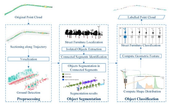
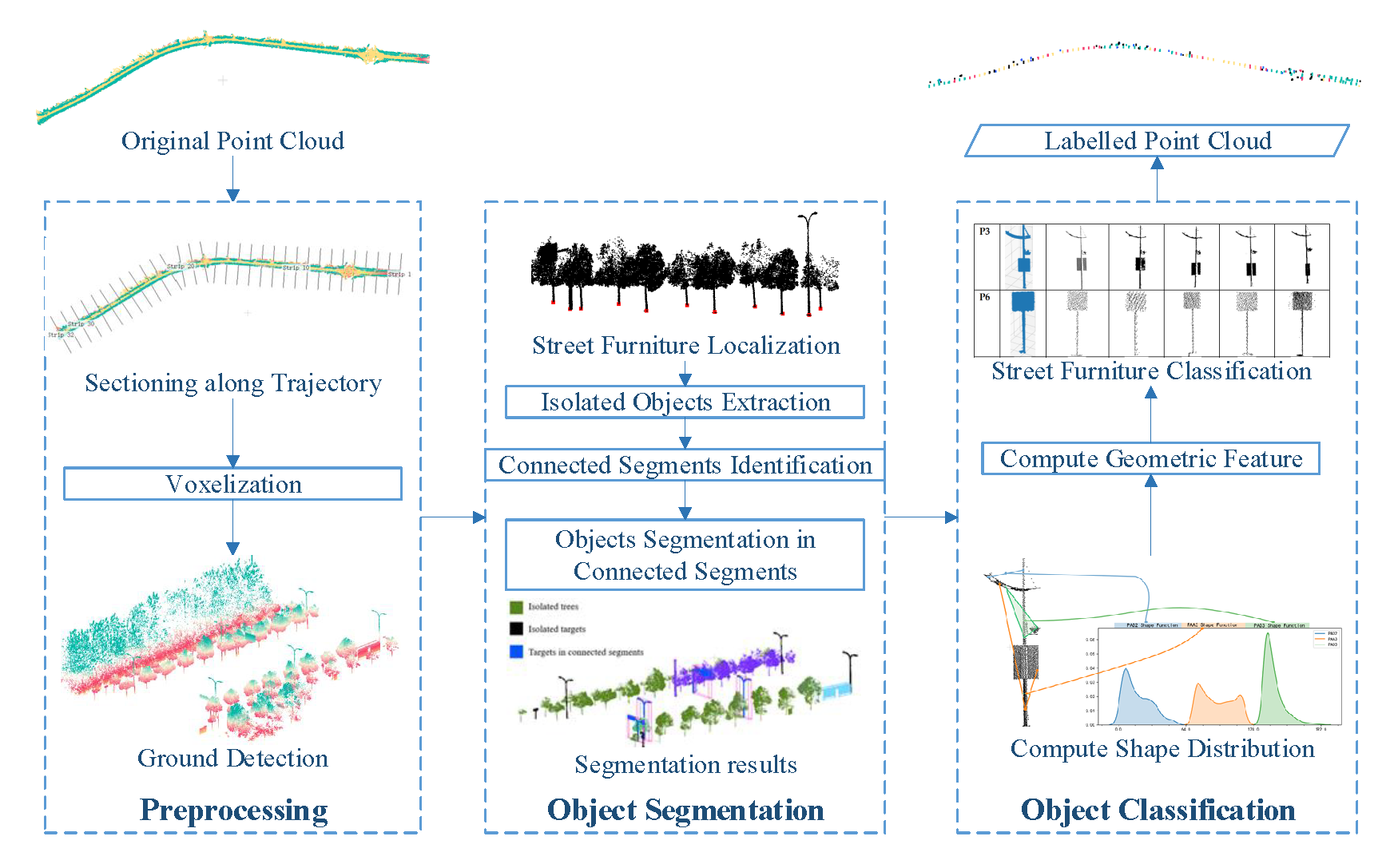
We investigated related work of classification methods after segmenting pole-like street furniture. Since the specific research field is under-researched, we tried to articulate the related work in a broader way to point cloud classification. Related methods of point cloud classification are categorized to segment-based classification methods [30,31,32] (closely related to the proposed classification method) and primitive-based methods [33,34,35,36,37,38,39,40,41,42]. The primitive-based methods are divided into two categories: point-based methods [33,34,35,36,37,38] and voxel-based methods or super-voxel based methods [39,40,41,42]. These primitive-based methods would also provide a clue for researchers who are interested in the classification of pole-like street furniture.
The point-based methods concentrate on point-level features, and attempt to classify each point to a specified class. Since the point-level features may find it difficult to preserve the smooth labeling for different objects, many researchers have tried to solve these problems by using an optimal scale to acquire more accurate geometric features [33,36] or combining contextual information [35,38]. Brodu et al. improved natural scene classification results by utilizing a multi-scale dimensionality criterion [34] while Weinmann et al. enhanced their classification results by experimenting with different neighbor sizes to find the optimal neighborhood [36]. Niemeyer et al. integrated a random forest classifier into a conditional random field (CRF) framework [35]. By this integration, they could take context feature into consideration and use many pointwise features as many other methods do. Li also incorporated contextual information to their classification method [38]. They enhanced the label smoothing in two ways: each point can collect sufficient neighborhood information to achieve an optimal graph; they improved the input label probability set by probabilistic label relaxation to make the labels more consistent with spatial context. The voxel or supervoxel-based methods attempt to reorganize the original point clouds into another form, namely voxels or supervoxels, and then operate the feature extraction and classification processes on the voxels or supervoxels. Supervoxel are usually constructed by incorporating color and intensity information since different parts of an object or different objects often have different color or intensity values. Huang and You introduced a point cloud classification based on a 3D convolutional neural network on the voxel-level [40]. Their network could be improved if multiple resolution voxels of the network can be utilized. Kang and Yang constructed super-voxels firstly as primitives based on similar geometric and radiometric properties [42]. After that, they also constructed point-based multi-scale visual features on similar geometric radiometric and radio metric properties. They integrated features from these two-level primitives, and utilized a combined classifier including Bayesian network and Markov random fields. By applying these tricks, they obtained locally smoothed and globally optimal classification results.
An object-based classification method is often established on the basis of a segmentation method. The point clouds are first segmented to meaningful segments. After extracting and selecting features from these segments, these segments are then classified to different categories. These methods can be classified into supervised learning methods [16,27,43,44,45,46] and unsupervised learning methods [23,24,32,47,48,49]. The supervised classification methods extract the overall features of the segments and train the classifier for object classification based on the extracted features. Golovinskiy et al. utilized a graph-cut method to locate and segment street furniture in urban scenes, and after that several classifiers were introduced to classify these segmented clusters [31]. Another researcher later projected the point cloud to the horizontal plane to build a feature image based on height information, and then segmentation, feature extraction and classification were applied to the feature images [43]. Recently, Binbin Xiang et al. introduced a set of new features to their segments, which were fed to four classifiers and produced good classification results [46]. For unsupervised learning strategies, either thresholding or matching techniques are utilized to classify segments. Aijazi et al. extracted geometric, color and intensity features, and configured several thresholding values to measure the similarity of the five classes of furniture [24]. Yokoyama et al. extracted features from their segments, which they used to measure the objects’ similarity to lampposts, traffic signs and utility poles [47]. Yu et al. performed road scene object detection based on similarity measures [48]. Shi et al. automatically classify segmented pole-like street furniture by 3D shape matching [23]. Wu et al. proposed a new method to retrieve lampposts based on shape retrieval and shape correspondence [32]. Schnabel et al. decomposed the furniture into different geometric primitives and built the topological structure of each element, after which targets are retrieved using the given prototypes [49]. Wang et al. introduced an interesting shape descriptor named Sigvox, which computes multilevel features of street furniture based on an octree structure. This shape descriptor is also utilized to perform street furniture recognition [50].
Although many algorithms have been proposed regarding pole-like street furniture segmentation and classification, most state-of-art methods still need further improvement in complicated scenes where furniture is connected to each other. Besides, most existing methods utilized machine learning or specific models to classify specified categories of pole-like street furniture within their scope, they need improvements to recognize more object classes. To overcome these drawbacks, this paper proposes a complete strategy for urban pole-like street furniture segmentation and classification using mobile LiDAR data by integrating multiple shape descriptor constraint.

3. Methodology

3.1. Overview

This section depicts the detailed workflow of the proposed methodology (Figure 1). The following steps are included: (1) preprocessing along trajectories including sectioning and ground extraction; (2) segmentation of the original point cloud to discrete poles and trees, and target object segmentation; (3) feature calculation and object classification based on the integrated feature descriptors. The details of each processing step of our method are described as follows.

3.2. Preprocessing along Trajectory

Huge data volumes and the complexity of urban street scenes will result in computation and memory load problems. To tackle these problems, we sectioned the original point clouds into small strips along the trajectory lines. Therefore, we use the vehicle trajectory data ( T ) to section the point clouds into a set of strips at an interval ( d ) [6]. To ensure that the objects in one strip will not be split into two parts, there also should be an overlapping zone for each strip.
The sectioned point clouds can be roughly classified into off-ground points, on-ground points, and ground points [47]. The point cloud data were then voxelized to perform ground extraction and later pole-like street furniture segmentation. The extraction targets of the proposed method are the street furniture that stand on or close to the ground. To select these objects, the ground points first need to be detected after voxelization. The ground is assumed to be relatively low in a local area and it sits lower than and vertical to the on-ground objects. Therefore, the ground can be detected by analyzing the relative height in a neighborhood and the vertically continuous height of each horizontally lowest voxel in the whole voxel set. Voxels that satisfy both conditions are recognized as ground voxels. The vertical continuity height is obtained using a vertical height analysis algorithm for voxels detailed in a previous study [25].
The detected ground voxels were back-projected to the original point cloud and the corresponding points and voxels were filtered from the original dataset. The following processing steps are applied to the remaining point cloud and voxel data.

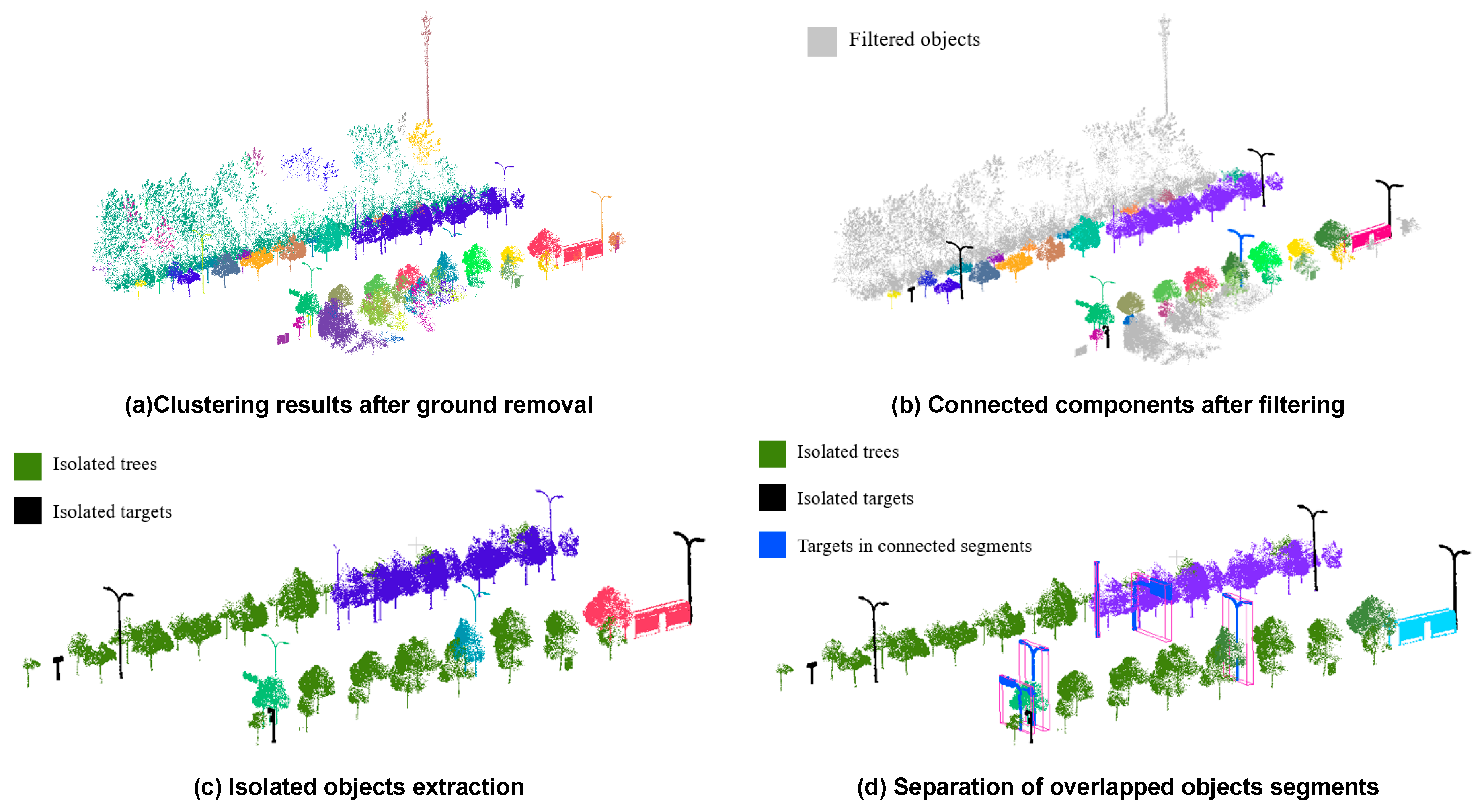
3.3. Segmentation of Target Street Furniture

After ground removal, the remaining point cloud still contains a variety of unwanted segments other than target pole-like street furniture, including cars on the street, buildings and trees beside the road. The whole remaining point cloud data were first clustered by using the DBCAN (Density-Based Spatial Clustering of Applications with Noise) algorithm, which results in discrete segments that represent different objects. The cars on the street can be filtered out based on their overall rectangular structures, while most buildings were filtered out based on height restrictions and planar structure extraction by using the RANSAC fitting algorithm. Then, the remaining point cloud data were subjected to the following processing steps to detect the target pole-like street furniture.

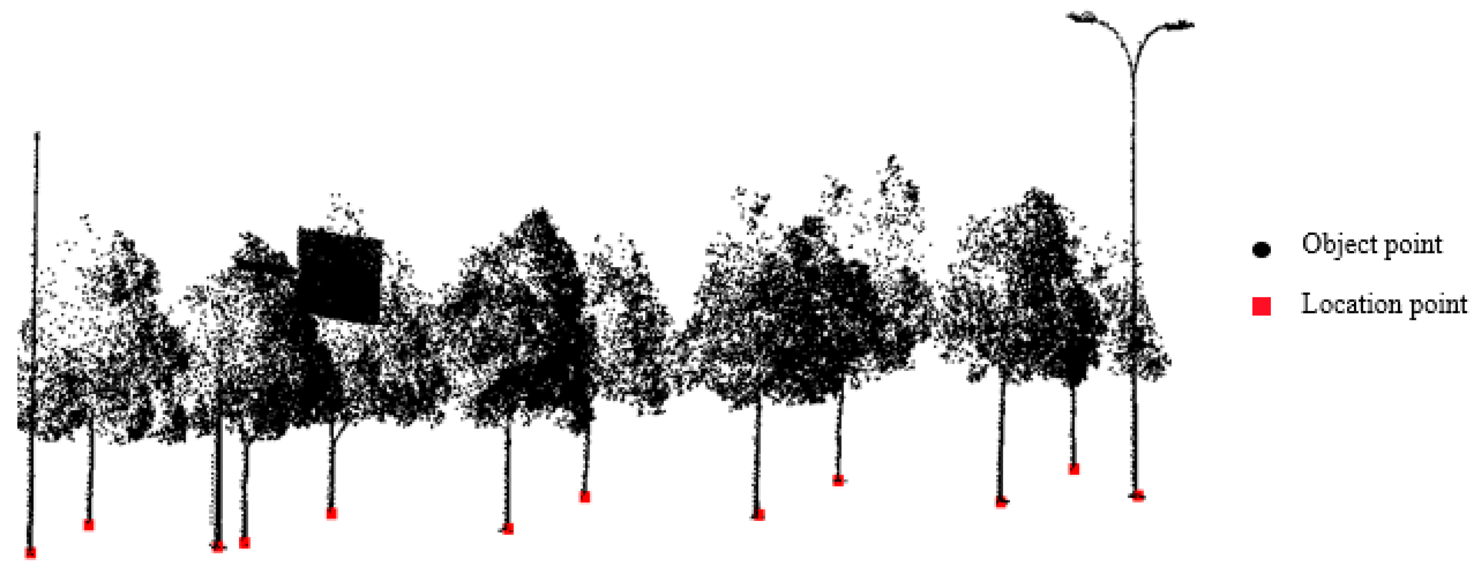
3.3.1. Street Furniture Identification

Pole-like street furniture is object that have a pole structure. In our database, the pole-like street furniture is higher than some of their surroundings. According to this feature, we implement a localization algorithm that identifies pole-like street furniture. A 3D density parameter d e i is designed to locate street furniture that is vertically high enough. We assume that a horizontal position with a large d e i is the position of a street object. For each voxel v i , the density parameter d e i can be formulated as follows:
d e i = { H v i ,                     d g r o u n d i < D t H v i / d g r o u n d i ,   d g r o u n d i D t
where d g r o u n d i is the distance from a voxel to its nearest ground point. H v i is the vertical continuous height of a horizontal voxel location. The parameter H v i can be calculated using the bottom-up tracing algorithm according to previous research [14]. This parameter will assign one voxel a high value that stems from the ground and has enough connecting voxels right above this voxel. These high-density neighboring voxels will later be merged and the voxel with the largest density value will be selected as the candidate street object location ( V c l ). Figure 2 gives an example of street object location detection result after back-projection from voxel to points, in which the black points are the street object point and the red point represent the geometric center of the detected location voxel.
These candidate locations are then analyzed and filtered out using a popular isolation analysis algorithm to select those isolated pole locations; this algorithm has been described in detail in previous research [25]. Additionally, the selection of the diameter of the inner cylinder D i n n e r is based on the maximum horizontal section size of the pole part of the target pole-like street furniture in real scenes, as discussed in previous research regarding isolation analysis [14,15,17,51]. Locations that have an isolated structure are recognized as candidate pole-like street furniture locations for further processing.

3.3.2. Connected Segments Identification

After the candidate pole-like street furniture locations were selected, the segments with these locations can then be classified as isolated pole-like street furniture, isolated trees and trees or poles that are connected with other objects. The isolated trees and pole-like street furniture are those segments with only one street object location voxel ( V c l ), while connected segments are those with more than one V c l . The isolated pole-like street furniture and trees can be differentiated using regular roughness measurements. Pole-like street furniture are man-made structures with regular structures, and they usually have low roughness values while trees are natural objects with relatively high roughness values (Equation (3)). The roughness values can be calculated based on the following equation:
r g h i = e 3 / e 1
where e 3 is the smallest eigenvalue and e 1 is the largest eigenvalue after performing principal component analysis. Isolated pole-like furniture and trees can be differentiated by thresholding the roughness values of the objects. 11 prototypes of street objects that depict the difference of point roughness values distribution is presented in the figure below (Figure 3). The point is colored by roughness values calculated by Equation (2), and the average roughness value of each object is labeled on corresponding object. We can easily select trees out from other pole-like street furniture just by finding objects with high average roughness values.

3.3.3. Resegmentation of Connected Objects

The connected segments that connect trees and pole-like street furniture need to be separated to extract the target objects. We introduce a density-based clustering algorithm to segment these connected objects [25]. This clustering algorithm contains two main steps: selecting the cluster centers and assigning the segment labels. The cluster center is the object location that is selected in the previous step. The 3D density value of each voxel is calculated based on Equation 10. We adopt the idea that point labels are more likely to be similar to a neighborhood that has higher density values [52]. In the proposed algorithm, the label of each voxel can be obtained by using the sequence of 3D density values in descending order. Every non-center voxel’s label is determined by using its neighboring voxel, which is the closest voxel that has a higher local density than the current voxel within a neighboring distance. Assume that the voxel set that is sorted with the local density in descending order is { m i } i = 1 N . The neighboring voxel index n m j of each voxel v i can be specified by the following formula:
ρ i = { H v i h i H i + p i p m a x ,                       d g r o u n d i < D t ( H v i h i H i + p i p m a x ) / d g r o u n d i ,   d g r o u n d i D t .
where h i is the vertical height of voxel v i , H v i i the vertical continuous height of a horizontal voxel location calculated the same way as in Equation (2), p m a x denotes the maximum number of points in one voxel and p i is the number of points in the current voxel v i . Below is a typical scene in an urban scene where trees and a lamppost are standing next to each other. Voxels from the tree trunks and pole part of the lamppost have high 3D density values while the tree crowns and the attachment part of the lamppost have voxels with low values (Figure 4).
Every non-center voxel’s label is determined by using its neighboring voxel, which is the closest voxel that has a higher local density than the current voxel within a neighboring distance. The whole voxels in the dataset are sorted in descending order of the 3D density values of each voxel. Assume that the voxel set that is sorted with the local density in descending order is { m i } i = 1 N . The neighboring voxel index n m j of each voxel v i can be specified by the following formula. In the equation, { V c l } is a set of street object locations
n m j = { argmin j < i { d m i m j } ,   i > 1 0 ,       i = 1   | | j { V c l }
After the clustering-based segmentation, trees and pole-like street furniture are separated. They can also be differentiated by the aforementioned roughness thresholding method. However, in some occasions the pole-like street furniture is not perfectly extracted because some points from trees are wrongly assigned to poles, as some of them are nested together. Therefore, we further implement a cleaning process to better extract the pole-like street furniture which will provide a fine and clean data source for the subsequent feature extraction and recognition process. We implement the cleaning by using ball falling method introduced from [15] to trace the pole part of the object. Figure 5 depicts a scenario before and after cleaning the noisy points. An overlapping segment with one lamppost and one tree was presented in Figure 5a. The lamppost was then segmented out using the clustering algorithm (Figure 5b), in which there are many noisy points around the pole part. The lamppost was then cleaned using the proposed method and we can obtain a more precise lamppost point cloud (Figure 5c).

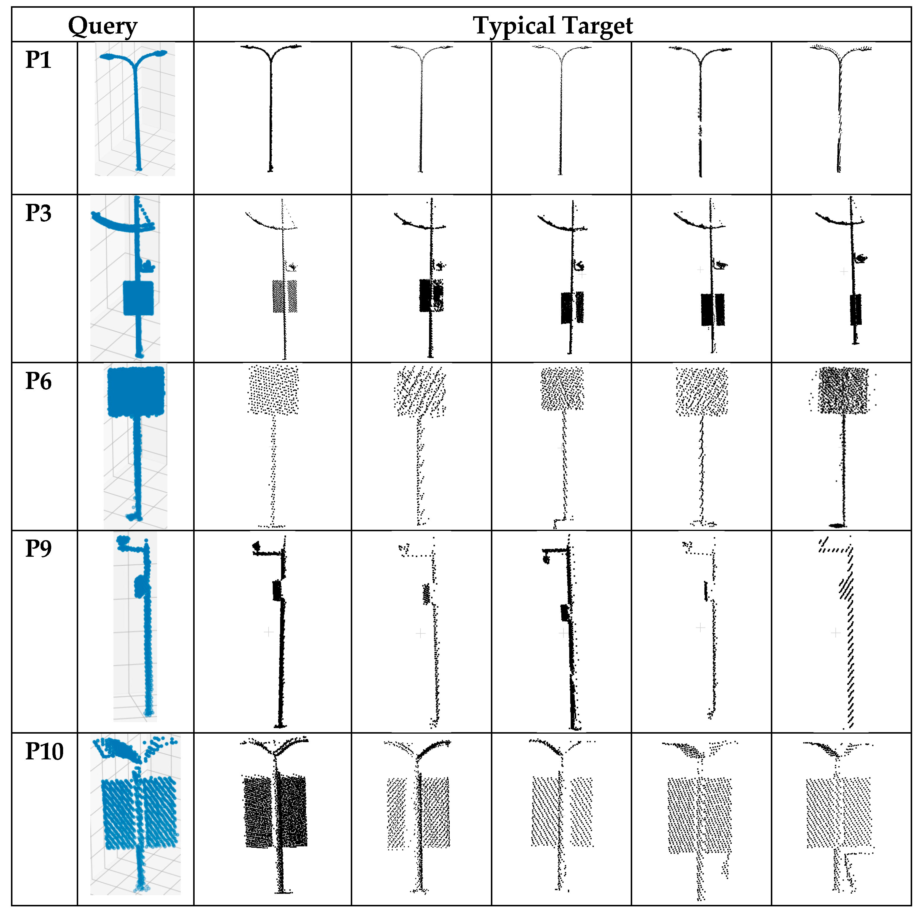
3.4. Object Classification based on Splitting Result of Pole-Like Street Furniture (SplitISC)

To differentiate different kinds of pole-like street furniture, an integrated shape constraint SplitISC is introduced. SplitISC combines three pole attachment-based shape distribution descriptors (PASD) and five geometric shape descriptors (GSD). The pole-like street furniture is first split into pole and attachment components to better compute and represent different features.

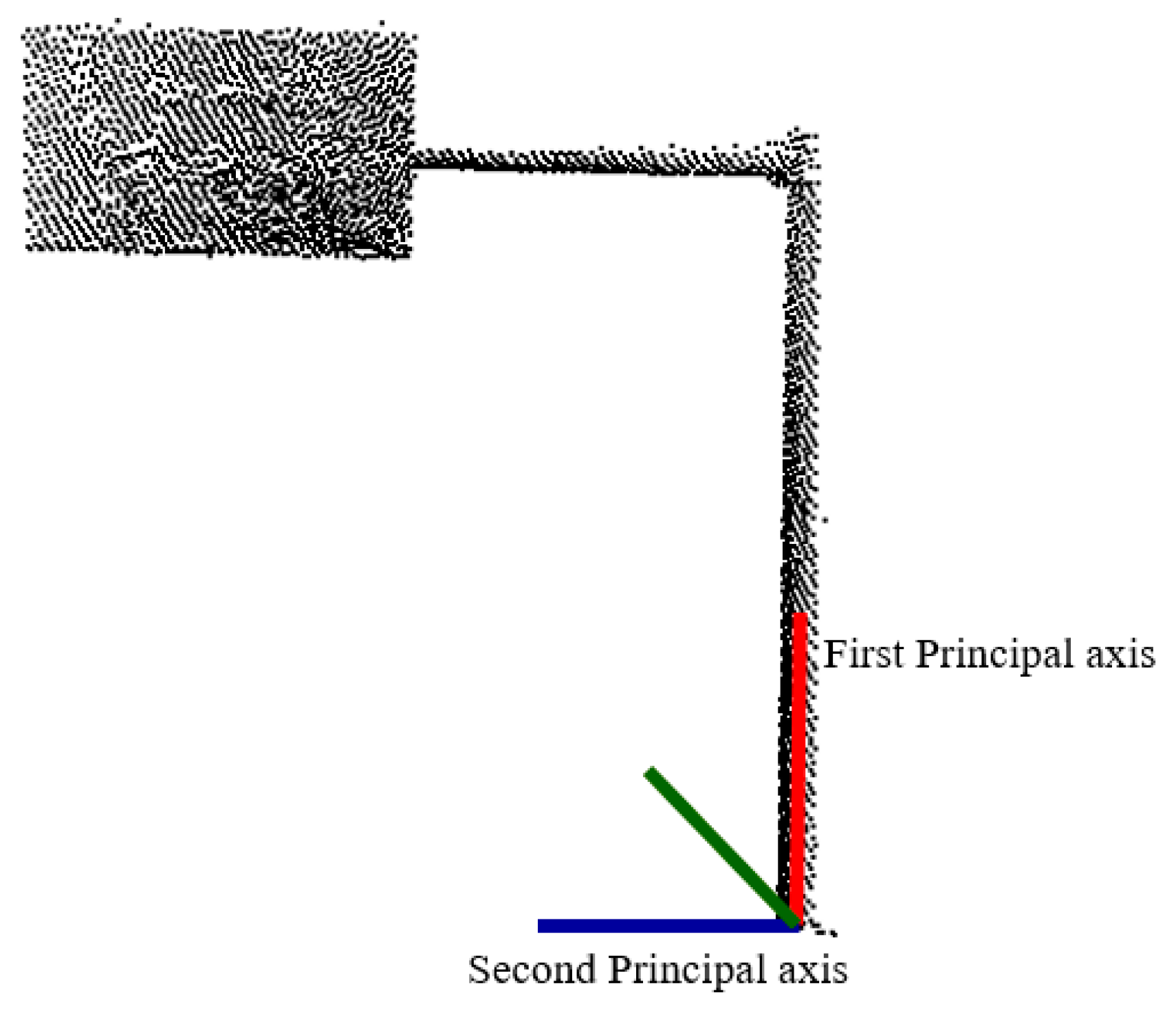
3.4.1. Pole Attachment-Based Shape Distribution Descriptors (PASD) estimation

To differentiate different kinds of pole-like street furniture, two kinds of shape descriptors are introduced: the PASD and the GSD. The pole-like street furniture is first split into pole and attachment components to compute and represent the different features more precisely.
(1) Pole-attachment-based shape distribution descriptor
The pole-attachment-based shape description descriptor builds new shape functions to better represent shape distribution. The pole-like street furniture is first split into poles components and attachments components and the shape functions are built by using the separated components. We conduct isolation analysis layer by layer from bottom to top on a pole-like street furniture to split the object to different parts. The pole-like street furniture splitting Algorithm 1 is presented below.
Algorithm 1: Pole-like street furniture splitting
Input:
C: point cloud cluster
P: pole part points (obtained from the cleaning step)
Parameters:
h l a y e r : layer height
{ p C i } : points in C at layer i
{ p P i } : points in P at layer i
maxz: z value of highest point in C
minz: z value of lowest point in C
i s o c o u n t : number of continuous isolated layers
Start:
Initialize with
h l o w : minz
h h i g h : h l o w + h l a y e r
Repeat
(1)
i s o c o u n t = 0, { p t e m p } = , i = 0
(2)
Select current layer points p C i = a r g z ( p h l o w )&&   a r g ( p < h h i g h )( p C )
(3)
Select current pole part points p P i = a r g z ( p h l o w )&&   a r g ( p < h h i g h )( p P )
(4)
Find { p P i } ‘s neighbours { p N i }
(5)
IF sizeof( { p N i } ) { p P i } < 3
(6)
Repeat
(7)
     p P i { p t e m p }
(8)
     i s o c o u n t = i s o c o u n t + 1, i = i + 1
(9)
     h l o w = h l o w + h l a y e r ,   h h i g h =   h h i g h +   h l a y e r
(10)
    Select current layer points p C i = a r g z ( p h l o w ) &&   a r g ( p < h h i g h )( p C )
(11)
    Select point of pole part p P i   = a r g z ( p h l o w ) &&   a r g ( p < h h i g h )( p P )
(12)
    Find { p P i } ‘s neighbours { p N i }
(13)
Until size of ( { p N i } ) size of { p P i } < 3
(14)
IF i s o c o u n t > 1:
(15)
     { p t e m p } { P P j }
(16)
     j = j + 1
Until h l o w m a x z
(17)
Remove points { P P j } from C, and obtain new point set C A
(18)
Perform DBCAN on C A to get attachment component set { P A j }
Output:
{ P P j } : pole part set
{ P A j } : attachment component set
A lamppost splitting example is presented below using the proposed spitting example (Figure 6). The left figure shows the original lamppost point cloud while the right figure shows the results after splitting out the lamppost. Different color represents different parts of pole-components and attachment-components.
(2) PASD
PASD is a combination of three shape functions, which enhance the original distance function (D2), angle function (A3) and area function (D3) [53]. We found that when the sample frequency surpassed a threshold value F s a m p l e s , the shape function became stable within every test data. Therefore, we randomly sampled the data F s a m p l e s times, and in each iteration, one random point from the pole components and two points from an attachment component of one pole-like street furniture were chosen to compute the following functions.
(1)
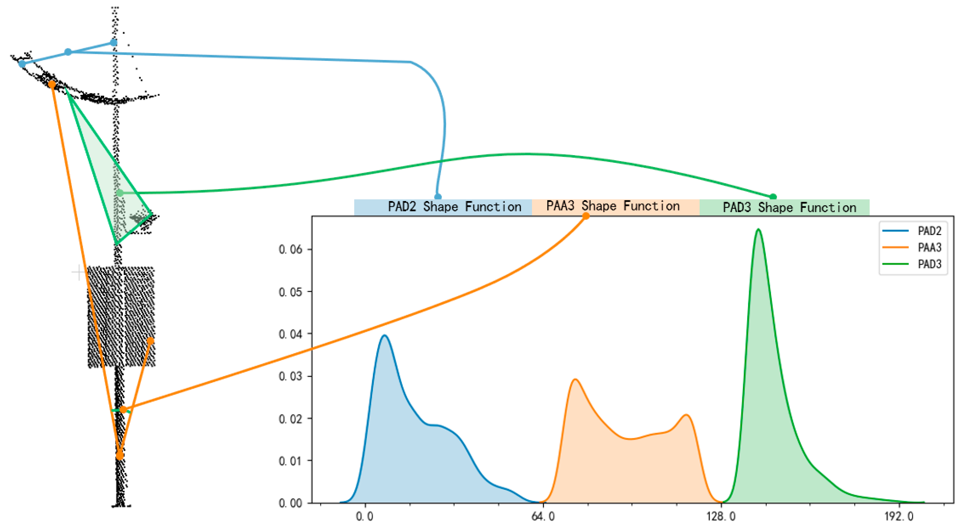
PAD2: PAD2 computes the distance between the pole component point and one point from the attachment component (Figure 7).
(2)
PAA3: PAA3 computes the angle between three points, one point from the pole and the remaining two from the attachments, which will be used to shape the horizontally expanding range of the pole-like street furniture.
(3)
PAD3: PAD3 computes the area of a triangle that is constructed by three points, consisting of one point from the pole and the remaining two from the attachments.
Each shape function is built with 64 bins, and they in all constitute a histogram of 192 values. Figure 7 shows a combinational shape function of pole-like street furniture.

3.4.2. Geometric Shape Descriptors (GSD) Estimation

The shape distribution descriptor can depict the overall shape distribution of an object. However, since it is invariant to the rotation and scale, we need to incorporate other shape descriptors to extract the real sized geometric features.
(1) Local coordinate system construction: to better estimate the geometry of a pole-like street furniture, we need to project the segments to a uniform local coordinate system. We introduce the principal component analysis (PCA) method to compute the axis direction of the local coordinate system. We project all the points from a segment to the XOY plane and assume that all projected points are represented by a point set P i , i { 1 , , k } . This approach allows us to build the following covariance matrix:
M = 1 k i = 1 k ( p i p ¯ ) · ( p i p ¯ ) T
in which k is the point amount of point set P i ; and p ¯ is the geometric center of P i , which can be calculated using the formula p ¯ = 1 k i = 1 k p i . By computing the covariance matrix, we can obtain two eigenvalues in descending order, which correspond to the eigenvectors { e 1 , e 2 } . Then, the eigenvector e 1 , corresponding to the larger eigenvalue λ 1 , is the principal direction of point set P i . We specify the object location in Section 3.3.1 as the origin of the coordinate system, the vertical location as the first axis, the principal direction as the second axis and the direction that is vertical to these two axes as the third axis. Figure 8 shows a sample of estimating the coordinate system for a traffic sign.
(2) GSD estimation: the pole-attachment-based shape distribution descriptor is scale invariant which means it does not contain size information. Thus, we incorporate geometric descriptor to take this information into consideration. Aside from height along the first principal axis ( H 1 ), width along the second axis ( W 2 ) and volume of the segment ( V ), many pole-like street furniture items in cities have strong symmetry, which is mainly centered on the pole on of the object. The symmetry of a pole-like street furniture is defined by the overlap area of the convex hull between both sides of the pole. After projecting the points from the original segment to the planned constructed by using the first and second axes, we can estimate the symmetry of the segment by using the following formula:
S y m m e t r y 2 D =   max ϕ ( S 1 i , S 2 ) max ( a r e a ( S 1 , S 2 ) )
where S 1   and   S 2 represent the point cloud beside each side of the first axis, and ϕ i ( S 1 , S 2 ) represent the overlapping area of the convex hull of S 1 and S 2 when S 1 rotates around the first axis i °( i ϵ { 1 ° , 2 ° 360 ° } ).
The compactness of an object if the object occupies enough space in its bounding box can be calculated based on the following equation:
Compact 3 D = v o l u m e ( V ) / v o l u m e ( B )
where v o l u m e ( V ) is the total volume of all the voxels of the segments and v o l u m e ( B ) represents the volume of the segment’s bounding box.

3.4.3. Object Recognition

Using the abovementioned shape descriptors, we introduce corresponding measures to calculate the similarity of two segments, which will be tested in our object retrieval experiment. Object recognition contains two objects: the first one is a template T and the second one is an instance P . The recognition criterion is based on both the shape distribution similarity and the geometric shape descriptor similarity. The shape distribution similarity of the template object and the instance object is specified as S S D ( T , P ) and the geometric shape descriptor similarity is denoted as S G S ( T , P ) . P is recognized as T when their similarity surpasses a threshold value. S S D ( T , P ) can be calculated using the Minkowski L N norms of the probability density functions (pdfs) [54], while S G S ( T , P ) can be calculated using Equation (9).
S ( T , P ) = ( S S D ( T , P ) + + S G S ( T , P ) ) / 2
S G S ( T , P ) = ( S H   ( T , P ) + S W ( T , P ) + S V ( T , P ) + S S y m m e t r y ( T , P ) + S Compact ( T , P ) ) / 5
where S H   ( T , P ) ,   S W ( T , P ) ,   S V ( T , P ) ,   S S y m m e t r y ( T , P ) ,   S Compact ( T , P ) represent similarity of H 1 , W 2 , V , S y m m e t r y 2 D ,   and   Compact 3 D values between template T and instance P, respectively.

4. Results

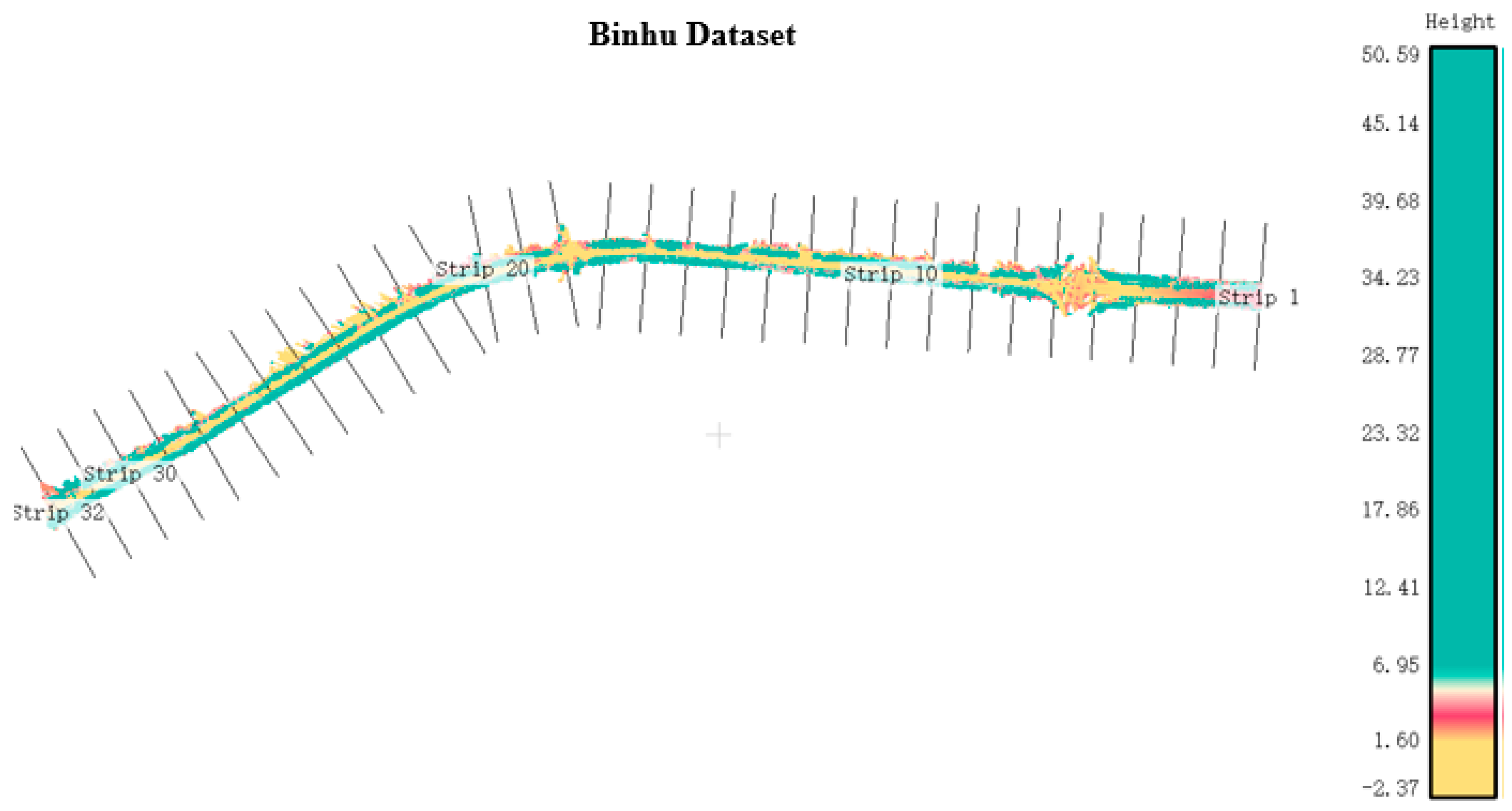
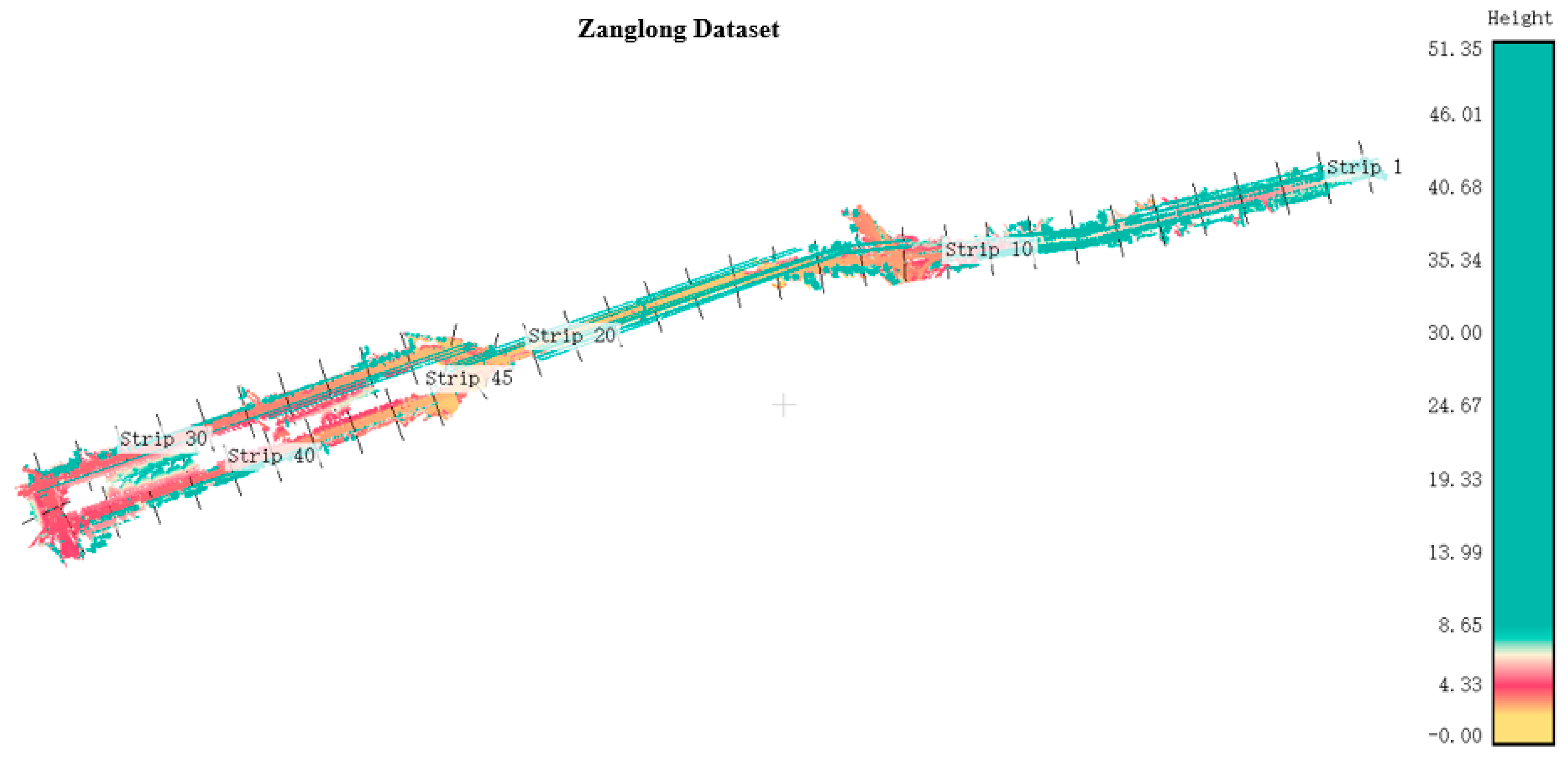
4.1. Dataset and Parameter Setting

To test the effectiveness and efficiency of the proposed method, we choose two test sites in Wuhan, a central city in China, to conduct the experiment. The point clouds were captured by a Lynx Mobile Mapping System, which consists of two laser scanners, one GPS (Global Positioning System) receiver and an inertial measurement unit. The frequency of both laser scanners was 100 kHz. The two test sites both contain different kinds of target street furniture.
The first dataset was collected along Binhu Road and is named the Binhu dataset. The maximum driving speed of this platform was 50 km/h. In this dataset, the pulse count, pulse number and reflectance were also collected. The survey area is approximately 2 km long, and more than 44 million points were collected. The point density is an average of approximately 293 points per square meter.
The second test site was another region of Wuhan. The dataset is collected along a 3.3 km stretch of the Zanglong road with different kinds of street furniture, and it is named the Zanglong dataset. In both datasets, the data were captured from the city streets at normal urban speed limits of 30–40 km/h. The dataset contains more than 57 million points with an average point density of 345 points per square meter. Detailed information of the two datasets, including the road length and number of points, is presented in Table 1.
Table 2 listed the key parameter configurations of the proposed algorithm for the two datasets. V is the voxel size for the voxelization in the preprocessing stage. The voxel size is an important parameter in the localization step, and it is mainly determined by point density. The density of mobile LiDAR data in each test site varies greatly both between the test sites and within each test site. The average point span for distant objects between scan lines in the test sites is approximately 0.15 m. To guarantee that distant objects have vertically continuous voxels in the segmentation step, the voxel size was set to two times the average point span, namely, V = 0.3 m. D i n t e r v a l is the interval for sectioning the original data along the trajectories. To section the experimental data into a number of blocks, we chose D i n t e r v a l = 80 m for both datasets. To prevent target objects from being split, we choose an overlapping distance D o v e r l a p = 5 meters, and repeated objects are merged in later processing steps. D t is a threshold value when computing 3D density value for each voxel in the segmentation step, which is configured based on the distance between attachment components of target pole-like street furniture and the ground. In our experiment, these components are 1.5 meters higher above the ground, thus this threshold value is configured as 1.5 m. D i n n e r is the diameter of the inner cylinder for isolation analysis of the segmentation stage, which is determined by the size of the pole part of the target. The roughness threshold value T r o u g h is a threshold value to differentiate trees from pole-like street furniture. The layer height parameter h l a y e r is the layer height in the pole-like street furniture splitting step. Sample frequency parameter F s a m p l e s depicts the iteration times for selecting points to build the proposed three shape functions in the classification stage. This value is configured as 10,000 since we found that when the sample frequency surpassed 10,000, the proposed shape function became stable in our datasets. The neighbor radius parameter R n e i g h b o r is the radius for searching neighbors when constructing the covariance matrix in the local coordinate system estimation step and in the roughness estimation step, which is also configured based on the point density as with the voxel size parameter.

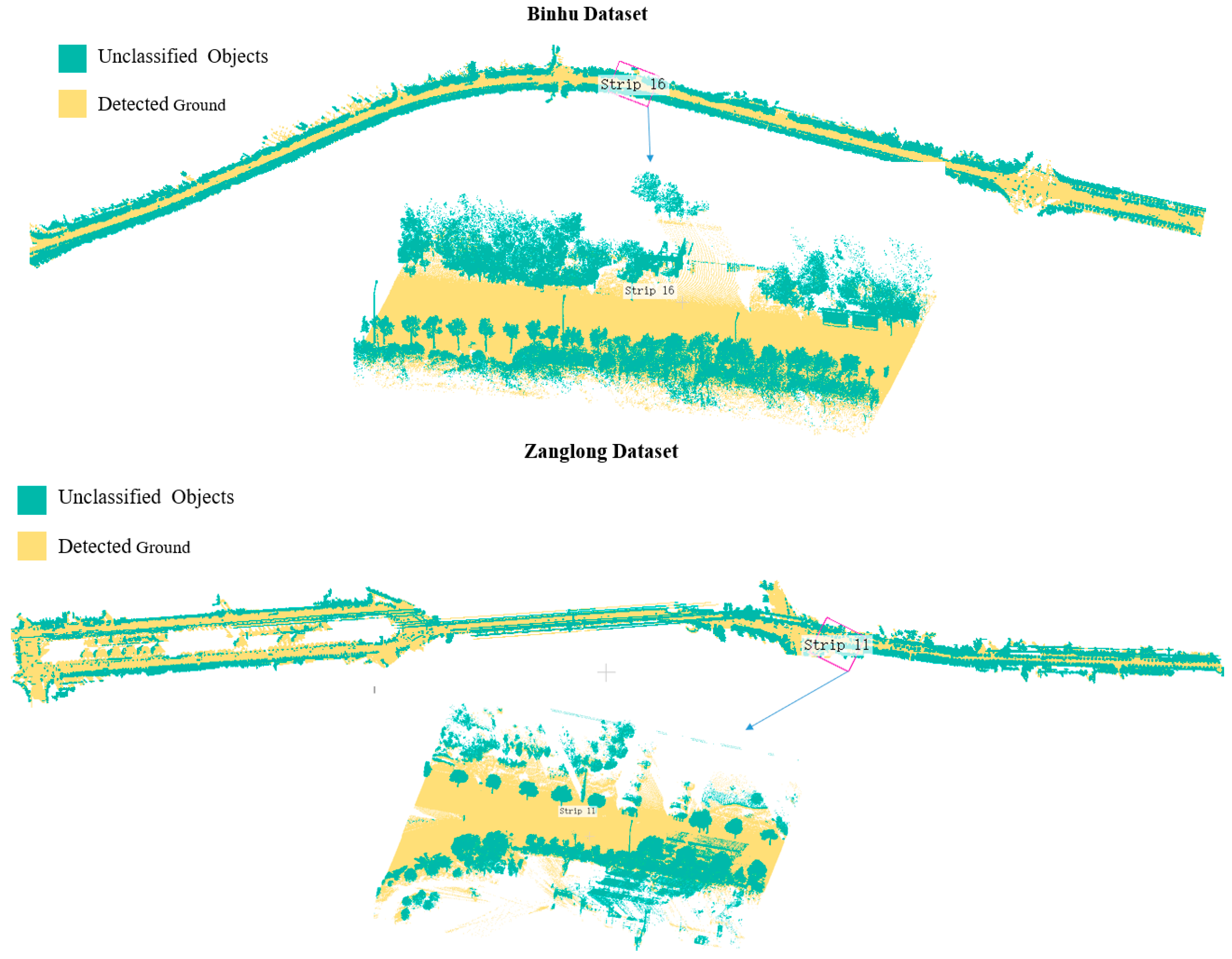
4.2. Evaluation of Sectioning and Ground Extraction Results

To section the experimental data into a number of blocks, we chose d = 80 m for both datasets. To prevent target objects from being split, we chose an overlapping distance of 5 meters, and repeated objects are merged in later processing steps. The Binhu dataset was sectioned into 32 strips, while the Zanglong dataset was sectioned into 45 strips (Figure 9).
The voxel size is an important parameter in the voxelization and localization processing step, and it is mainly determined by the point density. The density of the mobile LiDAR data in each test site varies greatly both between the test sites and within each test site. The average point span for distant objects between scan lines in the test sites was approximately 0.15 m. To guarantee that distant objects have vertically continuous voxels in the segmentation step, the voxel size was set to two times the average point span, namely, 0.3 m. The numbers of voxels generated in the voxelization step were 2.04 million and 2.16 million in the Binhu and Zanglong datasets, respectively, with compression rates (1 – number of voxels containing data/number of original points) of 96.4% and 95.1%, respectively. After voxelization, the ground can then be detected based on the voxels generated.
The ground detection operations are applied to each strip. The vertical height of each voxel was first estimated for every voxel in each road strip. Then, the height difference between the current voxel and a voxel within a certain neighborhood was calculated. Then, the voxels with small vertical height values (1 m) and height differences (0.5 m) were categorized as ground points and removed. The results for the two selected strips in each dataset after back-projection from the voxels to the points are presented in Figure 10, in which the yellow colored points are the detected ground points from the proposed method.

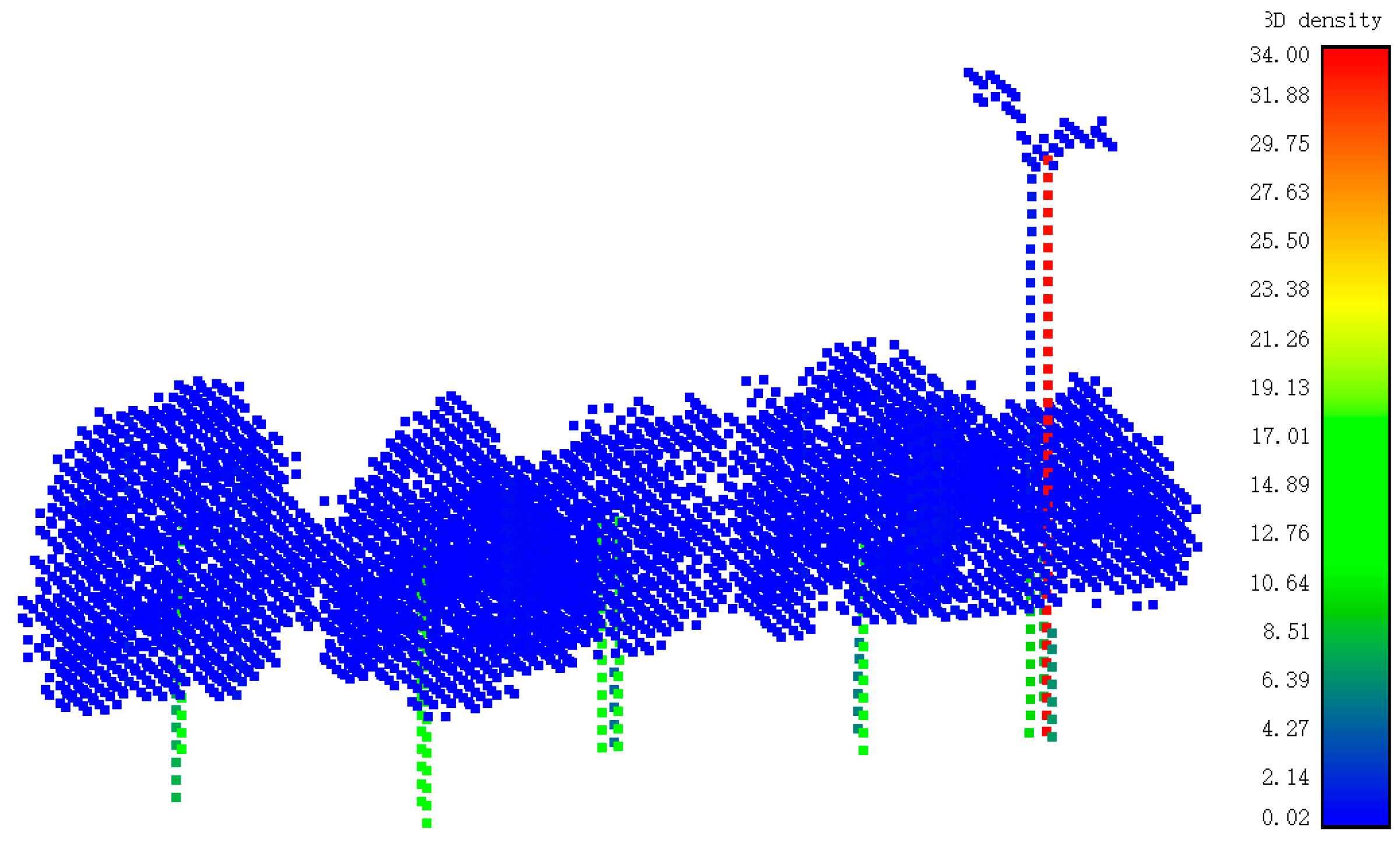
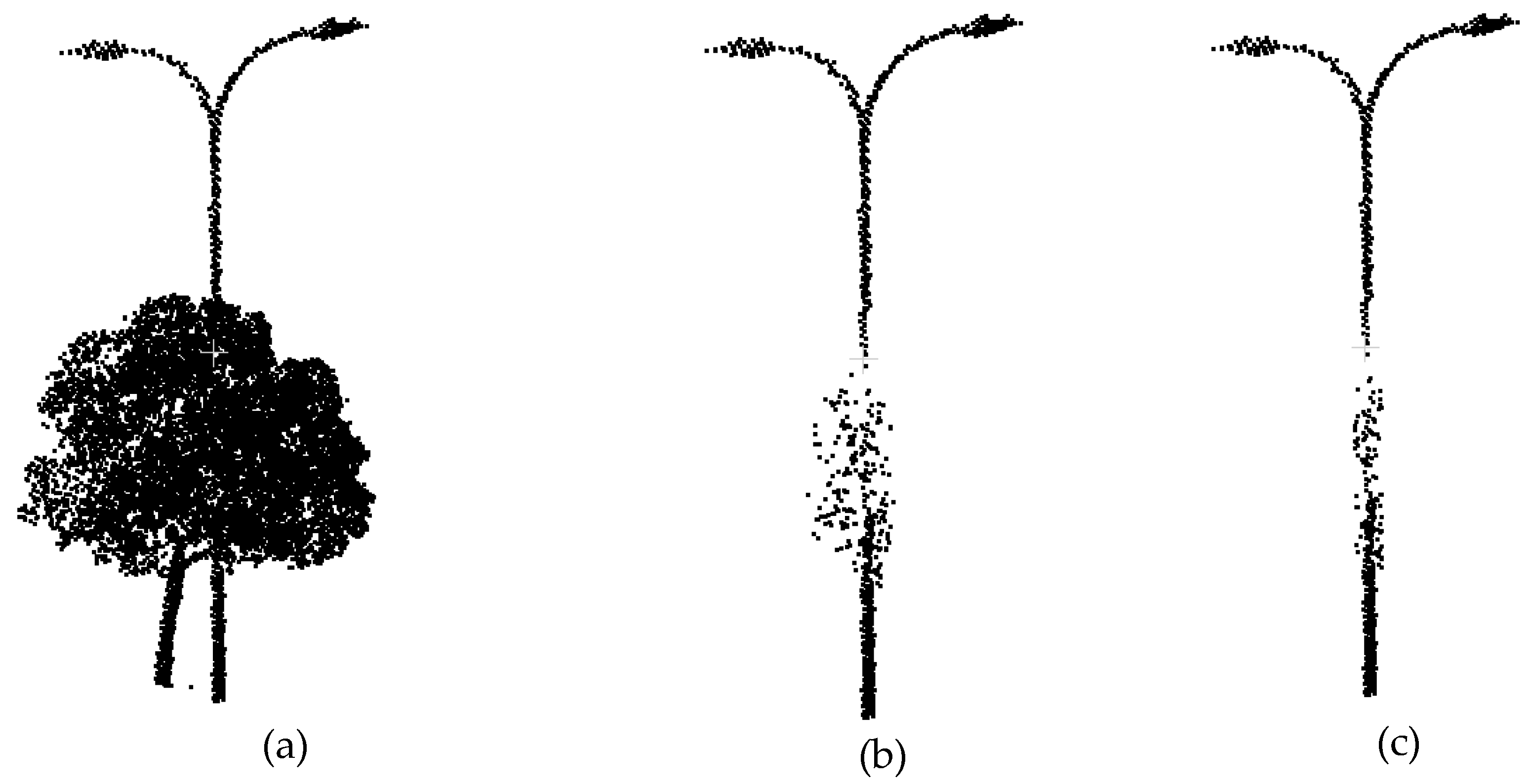
4.3. Qualitative Evaluation of the Object Segmentation Algorithm

The pole-like street furniture extraction procedure of one typical road strip in the Binhu dataset is presented in Figure 11. After ground removal, the above ground components were found by applying the DBSCAN algorithm. This clustering algorithm outputs many segments (differentiated by different colors) that represent part of an object, an objects or several objects (Figure 11a). The components include isolated trees, connected trees poles and one bus stop. We then filter out the components that are obviously not our targets, such as those that are colored gray in Figure 11b. The remaining components include isolated trees, poles that are connected with trees and isolated pole-like street furniture. After the isolation analysis, the isolated poles were detected, as is shown in Figure 11c, and the detected isolated poles are colored black in the figure. The isolated trees can also be detected in this stage and are colored green in Figure 11c. The 4 remaining components that contain poles that are connected to other objects need further separation. Two components contain both one lamppost and one traffic sign and the last one contains one lamppost. After applying the separation algorithm to each component, the pole-like street furniture was all correctly separated, as is shown in Figure 11d (the isolated poles are colored black, the separated poles from the poles that are connected with trees are colored blue and the isolated trees are colored green).

4.4. Quantative Evaluation of the Object Segmentation Algorithm

Two measures, the completeness C P and the correctness C R , are introduced to evaluate the object detection results as follows:
C P = T P / V P
C R = T P / A P
where TP, VP and AP are (1) the number of correct pole targets from the detected road pole-like street furniture obtained by using the proposed method, (2) the number of detected road poles collected by using the artificial visual interpretation representing the ground truth, and (3) the number of detected road poles obtained by using the proposed method.
Table 3 depicts the results for the two different test sites for different kinds of road poles. For the Binhu dataset, 152 objects were extracted, of which 127 were pole-like street furniture. The total number of ground truth pole-like street furniture from the visual inspection was 133. The completeness and correctness for the dataset were 95.5% and 83.6%, respectively. For the Zanglong dataset with 182 ground truth pole-like street furniture, 189 segments were extracted, and 172 of them were pole-like street furniture. The corresponding completeness and correctness were 94.5% and 91.0%, respectively. It can be concluded that the proposed method achieved high completeness but low correctness in both test areas. Figure 12 shows part of the ground detection and pole-like street furniture extraction results from both datasets. In Figure 12a, two tree trunks are falsely detected as pole-like street furniture because they are both shaped like poles. Many similar tree trunks with branches are wrongly detected as pole-like street furniture because the trees that are far away that are located behind the trees in the front are only partially scanned by the laser scanner, which is the major cause for the low correctness for both datasets (Figure 12a). Additionally, partially scanned objects inside buildings can also be wrongly detected as pole-like street furniture. It is true that the CR values in two datasets would greatly improve if we remove all these false results before classification. However, since the shapes and point densities of different target street furniture may vary a lot, we still need further improvement to eliminate all these false segmentation results without reducing CP values. We need to reach a compromise between target diversity and segmentation accuracy. Fortunately, our classification algorithm is able to get rid of these wrongly detected poles from our classification results. In Figure 12b, two undetected targets are selected out. The lower bushes surrounding them affected the isolation analysis procedure and thus are missed in the proposed extraction algorithm (Figure 12b).

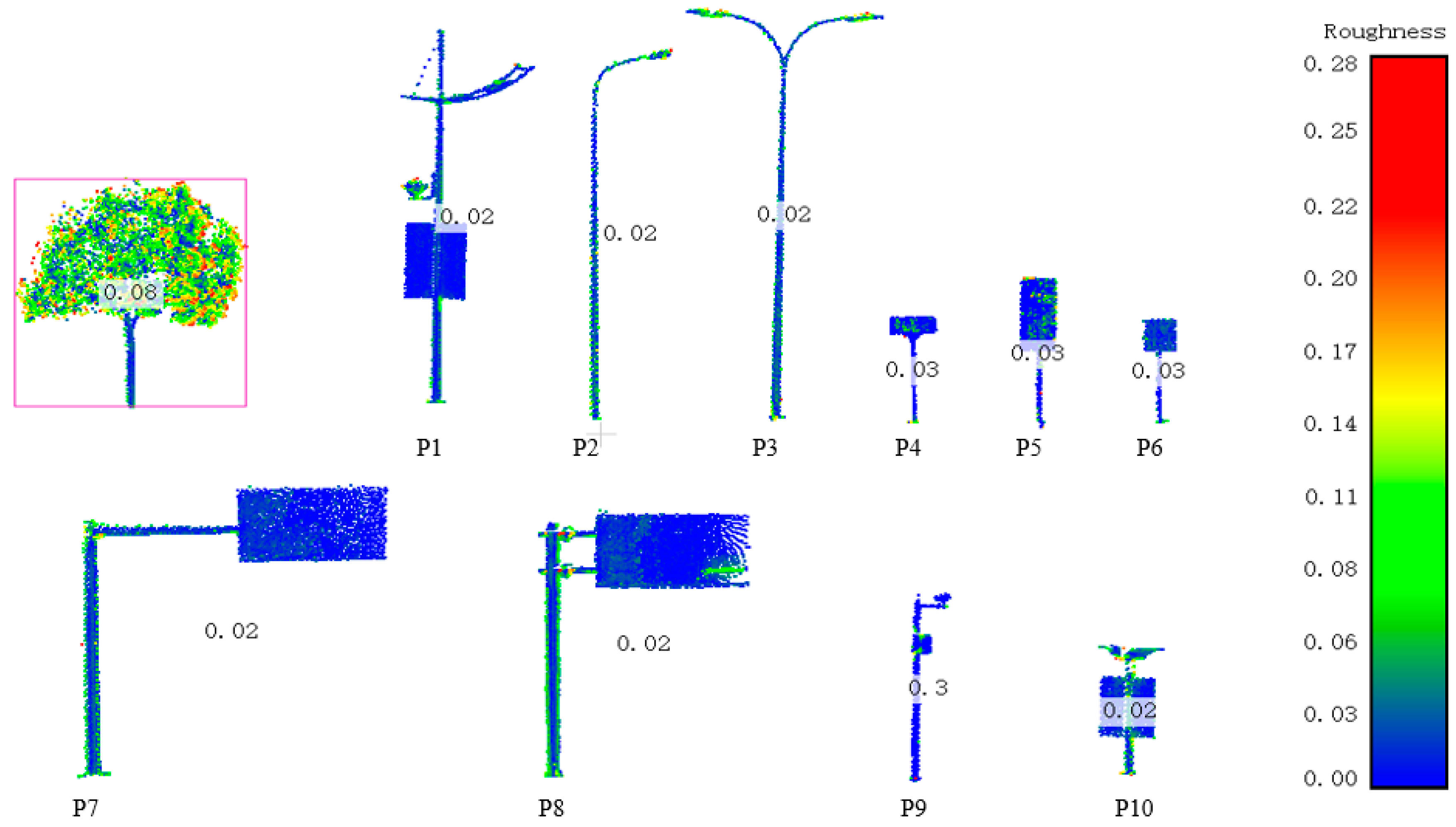
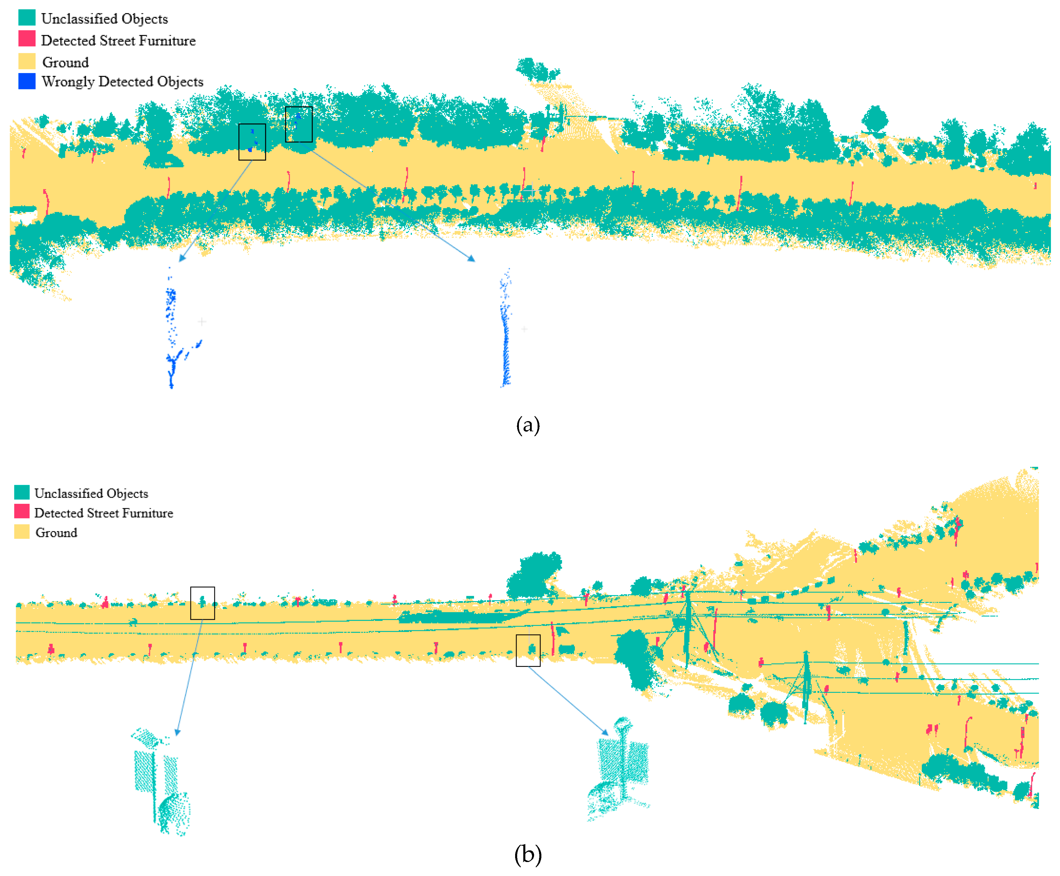
4.5. Qualitative Evaluation of the Object Recognition Algorithm

Ten prototypes of objects are selected and numbered to evaluate the proposed recognition algorithm. The 10 prototypes are presented in an above-mentioned figure (Figure 3).where the name below each prototype represent their number. The prototypes include 3 classes of lampposts, 5 classes of traffic signs, one class of surveillance cameras and one class of billboards. Five typical retrieval samples of these 10 prototypes are selected to show the performance of the proposed recognition algorithm in Figure 13. The left-hand figures are the queried point cloud prototype, and the results are presented on the right side of each prototype in order of their similarity values. It can be seen in the figures that the proposed method can retrieve samples with different point densities. Besides, slight occlusions in the pole part (recognition result of P1) and small amount of noisy points around the pole part are also tolerable using the proposed method (recognition result of P10).

4.6. Quantitative Evaluation of the Object Recognition Algorithm and a Comparative Study

To measure the results of the proposed method, we introduce three measurements, including completeness, correctness and quality. By visual inspection of other unrelated experimenters, the pole-like street furniture database was built and labeled. Table 4 shows the overall recognition results for 10 different prototypes of pole-like street furniture using the proposed method and traditional shape descriptor method (GHA) method (discussed in Section 5.2). The proposed method integrated PASD and GSD to recognize different protypes of objects. The correctness values for both datasets were over 93%, indicating that the proposed method can correctly detect target street furniture. The overall completeness values for both datasets using the proposed methods exceeded 96%, which means that both methods can completely detect targeted pole-like street furniture. The quality of the proposed method in the two datasets both exceeded 90% with the proposed method.

5. Discussion

5.1. Time Performance

The proposed algorithm was implemented in Python with a single thread on a PC with an Intel Core i7 − 7700 CPU. The CPU clock frequency was 3.60 GHz, and the memory size was 16 GB. The time cost at each stage of our method is shown in Table 5. The time costs of each processing step depended on many parameters, such as the input data volume and the algorithm complexity. The preprocessing time for Binghu Dataset and Zanglong Dataset were 781 s and 886 s, respectively. Time performance analysis revealed that the proposed algorithm provided a promising solution for pole-like street furniture segmentation and classification of mobile LiDAR point clouds, and achieved acceptable computational complexity. It can be concluded that time cost of every processing step of the Binhu dataset is less than that of the Zanglong dataset. The two datasets both have a total processing time cost of less than fifteen minutes for the whole workflow, which means that the proposed strategy is effective and capable for mass point clouds processing.

5.2. Comparison with Previous Methods

The proposed method can automatically segment pole-like street furniture and recognize different types of them semi-automatically. It is not straightforward to compare the proposed classification method to previous methods since different methods concentrate on different road conditions and are based on different data with different data accuracies. We attempted to compare the recognition results with the geometric histogram approach based on the original shape distribution method (GHA) [31]. The GHA method achieved much lower quality in Zanglong dataset (Figure 14). The proposed method outperforms the GHA method for both datasets considering the correctness measurement. In the Binhu dataset, the overall correctnessvalue increased from 90.6% to 98.9%, and in the Zanglong dataset, the value was enhanced from 70.9% to 93.6%, showing that the proposed method had fewer wrongly retrieved instances in its results. We analyzed some typical scenarios where the proposed method outperforms the GHA method (Figure 14). Different colors represent different components after the splitting procedure. The first and second row are the false recognition results using the GHA method when retrieving prototypes P9 and P4, respectively. After comparing recognition results of each type of object with two different methods, we found that the overall correctness values in the Zanglong dataset using the GHA method were much lower than those with the proposed method for two reasons. First of all, there were many unwanted tree trunks with branches and other poles which were wrongly recognized as pole-like street furniture prototypes (Figure 14a–c). Second, the original method did not take the real size of an object into consideration which led to the low correctness values for several kinds of traffic signs (Figure 14d–f).

6. Conclusions

In this paper, we presented a complete workflow for the extraction and recognition of pole-like street furniture from mobile LiDAR point clouds, including (1) an automatic ground-filtering algorithm to detect and filter ground points; (2) a 3D density-based segmentation method to segment target pole-like street furniture; (3) a novel method to split pole-like street furniture into pole parts and attachments; and (4) a retrieval method that depends on an improved object shape distribution descriptor, which takes objects’ structures into consideration. The proposed workflow was tested and evaluated by using two test datasets. The object extraction step shows that we can detect target objects at rates of over 94% in both datasets, and the overall completeness values of the retrieval step using the proposed method were over 96%. We compared the proposed SplitISC with the traditional shape descriptor method (GHA) in the object recognition procedure. The proposed method showed better results in both datasets. Besides, our approach only uses the coordinates of point clouds, and is also robust when detecting objects in overlapped regions. The experimental analysis conveyed the following conclusions:
1. The 3D density feature is a robust feature to localize target pole-like street furniture. The segmentation based on the localization result and 3D density feature performs well not only when targets are isolated but also when they are connected to trees.
2. The recognition rate can be improved by utilizing the proposed SplitISC including three enhanced shape distribution descriptors (PAD2, PAA3, PAD3) and five geometric shape descriptors (height along the first principal axis ( H 1 ), width along the second axis ( W 2 ), and volume of the segment ( V ), Symmetry and Compactness descriptors). The performance of the proposed method surpasses the original shape distribution method when we take the real size of street furniture into consideration.
In our future work, we will focus on some of the limitations of the proposed method; for example, how to improve the segmentation accuracy in more complicated situations; how to eliminate wrongly detected poles that originate from partially scanned tree trunks; or how to increase the number of target classes for segmentation and classification.

Author Contributions

Y.L., S.T., R.G., W.W., and X.L., contributed to the design and implementation of the proposed method, L.X., and W.X. helped collected the data, S.T. and Y.W. contributed to the analysis and processing of the data, Y.L. wrote the article.

Funding

This research was funded by the Natural Science Foundation of China (41901329, 41971354, 41971341, 41801392), the China Postdoctoral Science Foundation(2018M643150), the Open Fund of Key Laboratory of Urban Land Resources Monitoring and Simulation (KF-2018-03-066, KF-2018-03-036) and the Shenzhen Science and Technology Innovation Commission (JCYJ20170412142144518, JCTJ20180305125131482).

Conflicts of Interest

The authors declare no conflict of interest.

References

  1. Cabo, C.; Ordoñez, C.; García-Cortés, S.; Martínez, J. An algorithm for automatic detection of pole-like street furniture objects from Mobile Laser Scanner point clouds. ISPRS J. Photogramm. Remote Sens. 2014, 87, 47–56. [Google Scholar] [CrossRef]
  2. Zai, D.; Li, J.; Guo, Y.; Cheng, M.; Lin, Y.; Luo, H.; Wang, C. 3-D road boundary extraction from mobile laser scanning data via supervoxels and graph cuts. IEEE Trans. Intell. Transp. Syst. 2017, 19, 802–813. [Google Scholar] [CrossRef]
  3. Xu, S.; Wang, R.; Zheng, H. Road Curb Extraction From Mobile LiDAR Point Clouds. IEEE Trans. Geosci. Remote Sens. 2017, 55, 996–1009. [Google Scholar] [CrossRef] [Green Version]
  4. Wen, C.; Sun, X.; Li, J.; Wang, C.; Guo, Y.; Habib, A. A deep learning framework for road marking extraction, classification and completion from mobile laser scanning point clouds. ISPRS J. Photogramm. Remote Sens. 2019, 147, 178–192. [Google Scholar] [CrossRef]
  5. Ma, L.; Li, Y.; Li, J.; Zhong, Z.; Chapman, M.A. Generation of Horizontally Curved Driving Lines in HD Maps Using Mobile Laser Scanning Point Clouds. IEEE J. Sel. Top. Appl. Earth Obs. Remote Sens. 2019, 1–15. [Google Scholar] [CrossRef]
  6. Jung, J.; Che, E.; Olsen, M.J.; Parrish, C. Efficient and robust lane marking extraction from mobile lidar point clouds. ISPRS J. Photogramm. Remote Sens. 2019, 147, 1–18. [Google Scholar] [CrossRef]
  7. Xu, S.; Xu, S.; Ye, N.; Zhu, F. Automatic extraction of street trees’ nonphotosynthetic components from MLS data. Int. J. Appl. Earth Obs. Geoinf. 2018, 69, 64–77. [Google Scholar] [CrossRef]
  8. Li, L.; Li, D.; Zhu, H.; Li, Y. A dual growing method for the automatic extraction of individual trees from mobile laser scanning data. ISPRS J. Photogramm. Remote Sens. 2016, 120, 37–52. [Google Scholar] [CrossRef]
  9. Zhong, L.; Cheng, L.; Xu, H.; Wu, Y.; Chen, Y.; Li, M. Segmentation of individual trees from TLS and MLS data. IEEE J. Sel. Top. Appl. Earth Obs. Remote Sens. 2016, 10, 774–787. [Google Scholar] [CrossRef]
  10. Li, F.; Lehtomäki, M.; Oude Elberink, S.; Vosselman, G.; Kukko, A.; Puttonen, E.; Chen, Y.; Hyyppä, J. Semantic segmentation of road furniture in mobile laser scanning data. ISPRS J. Photogramm. Remote Sens. 2019, 154, 98–113. [Google Scholar] [CrossRef]
  11. Li, F.; Oude Elberink, S.; Vosselman, G. Pole-Like Road Furniture Detection and Decomposition in Mobile Laser Scanning Data Based on Spatial Relations. Remote Sens. 2018, 10, 531. [Google Scholar] [CrossRef] [Green Version]
  12. Zheng, H.; Wang, R.; Xu, S. Recognizing Street Lighting Poles From Mobile LiDAR Data. IEEE Trans. Geosci. Remote Sens. 2017, 55, 407–420. [Google Scholar] [CrossRef]
  13. Soilán, M.; Riveiro, B.; Martínez-Sánchez, J.; Arias, P. Traffic sign detection in MLS acquired point clouds for geometric and image-based semantic inventory. ISPRS J. Photogramm. Remote Sens. 2016, 114, 92–101. [Google Scholar] [CrossRef]
  14. Li, L.; Li, Y.; Li, D. A method based on an adaptive radius cylinder model for detecting pole-like objects in mobile laser scanning data. Remote Sens. Lett. 2016, 7, 249–258. [Google Scholar] [CrossRef]
  15. Wu, F.; Wen, C.; Guo, Y.; Wang, J.; Yu, Y.; Wang, C.; Li, J. Rapid localization and extraction of street light poles in mobile LiDAR point clouds: A supervoxel-based approach. IEEE Trans. Intell. Transp. Syst. 2016, 18, 292–305. [Google Scholar] [CrossRef]
  16. Rodríguez-Cuenca, B.; García-Cortés, S.; Ordóñez, C.; Alonso, M. Automatic detection and classification of pole-like objects in urban point cloud data using an anomaly detection algorithm. Remote Sens. 2015, 7, 12680–12703. [Google Scholar] [CrossRef]
  17. Brenner, C. Extraction of features from mobile laser scanning data for future driver assistance systems. In Advances in GIScience; Springer: Berlin/Heidelberg, Germany, 2009; pp. 25–42. [Google Scholar]
  18. Li, Y.; Wang, W.; Tang, S.; Li, D.; Wang, Y.; Yuan, Z.; Guo, R.; Li, X.; Xiu, W. Localization and Extraction of Road Poles in Urban Areas from Mobile Laser Scanning Data. Remote Sens. 2019, 11, 401. [Google Scholar] [CrossRef] [Green Version]
  19. Yang, B.; Dong, Z. A shape-based segmentation method for mobile laser scanning point clouds. ISPRS J. Photogramm. Remote Sens. 2013, 81, 19–30. [Google Scholar] [CrossRef]
  20. Yang, B.; Dong, Z.; Zhao, G.; Dai, W. Hierarchical extraction of urban objects from mobile laser scanning data. ISPRS J. Photogramm. Remote Sens. 2015, 99, 45–57. [Google Scholar] [CrossRef]
  21. Yang, B.; Liu, Y.; Dong, Z.; Liang, F.; Li, B.; Peng, X. 3D local feature BKD to extract road information from mobile laser scanning point clouds. ISPRS J. Photogramm. Remote Sens. 2017, 130, 329–343. [Google Scholar] [CrossRef]
  22. Ordóñez, C.; Cabo, C.; Sanz-Ablanedo, E. Automatic Detection and Classification of Pole-Like Objects for Urban Cartography Using Mobile Laser Scanning Data. Sensors 2017, 17, 1465. [Google Scholar] [CrossRef] [PubMed] [Green Version]
  23. Shi, Z.; Kang, Z.; Lin, Y.; Liu, Y.; Chen, W. Automatic Recognition of Pole-Like Objects from Mobile Laser Scanning Point Clouds. Remote Sens. 2018, 10, 1891. [Google Scholar] [CrossRef] [Green Version]
  24. Aijazi, A.; Checchin, P.; Trassoudaine, L. Segmentation based classification of 3D urban point clouds: A super-voxel based approach with evaluation. Remote Sens. 2013, 5, 1624–1650. [Google Scholar] [CrossRef] [Green Version]
  25. Li, Y.; Li, L.; Li, D.; Yang, F.; Liu, Y. A density-based clustering method for urban scene mobile laser scanning data segmentation. Remote Sens. 2017, 9, 331. [Google Scholar] [CrossRef] [Green Version]
  26. Xu, Y.; Yao, W.; Tuttas, S.; Hoegner, L.; Stilla, U. Unsupervised segmentation of point clouds from buildings using hierarchical clustering based on gestalt principles. IEEE J. Sel. Top. Appl. Earth Obs. Remote Sens. 2018, 11, 4270–4286. [Google Scholar] [CrossRef]
  27. Lin, Y.; Wang, C.; Zhai, D.; Li, W.; Li, J. Toward better boundary preserved supervoxel segmentation for 3D point clouds. ISPRS J. Photogramm. Remote Sens. 2018, 143, 39–47. [Google Scholar] [CrossRef]
  28. Xu, Y.; Sun, Z.; Hoegner, L.; Stilla, U.; Yao, W. Instance Segmentation of Trees in Urban Areas from MLS Point Clouds Using Supervoxel Contexts and Graph-Based Optimization. In Proceedings of the 2018 10th IAPR Workshop on Pattern Recognition in Remote Sensing (PRRS), Beijing, China, 19–20 August 2018; pp. 1–5. [Google Scholar]
  29. Xu, S.; Ye, N.; Xu, S.; Zhu, F. A supervoxel approach to the segmentation of individual trees from LiDAR point clouds. Remote Sens. Lett. 2018, 9, 515–523. [Google Scholar] [CrossRef]
  30. Guan, H.; Yu, Y.; Li, J.; Liu, P. Pole-like road object detection in mobile LiDAR data via supervoxel and bag-of-contextual-visual-words representation. IEEE Geosci. Remote Sens. Lett. 2016, 13, 520–524. [Google Scholar] [CrossRef]
  31. Golovinskiy, A.; Kim, V.G.; Funkhouser, T. Shape-based recognition of 3D point clouds in urban environments. In Proceedings of the 2009 IEEE 12th International Conference on Computer Vision, Kyoto, Japan, 29 September–2 October 2009; pp. 2154–2161. [Google Scholar]
  32. Yu, Y.; Li, J.; Guan, H.; Wang, C.; Yu, J. Semiautomated Extraction of Street Light Poles From Mobile LiDAR Point-Clouds. IEEE Trans. Geosci. Remote Sens. 2015, 53, 1374–1386. [Google Scholar] [CrossRef]
  33. Brodu, N.; Lague, D. 3D terrestrial lidar data classification of complex natural scenes using a multi-scale dimensionality criterion: Applications in geomorphology. ISPRS J. Photogramm. Remote Sens. 2012, 68, 121–134. [Google Scholar] [CrossRef] [Green Version]
  34. Lin, C.-H.; Chen, J.-Y.; Su, P.-L.; Chen, C.-H. Eigen-feature analysis of weighted covariance matrices for LiDAR point cloud classification. ISPRS J. Photogramm. Remote Sens. 2014, 94, 70–79. [Google Scholar] [CrossRef]
  35. Niemeyer, J.; Rottensteiner, F.; Soergel, U. Contextual classification of lidar data and building object detection in urban areas. ISPRS J. Photogramm. Remote Sens. 2014, 87, 152–165. [Google Scholar] [CrossRef]
  36. Weinmann, M.; Jutzi, B.; Hinz, S.; Mallet, C. Semantic point cloud interpretation based on optimal neighborhoods, relevant features and efficient classifiers. ISPRS J. Photogramm. Remote Sens. 2015, 105, 286–304. [Google Scholar] [CrossRef]
  37. Landrieu, L.; Raguet, H.; Vallet, B.; Mallet, C.; Weinmann, M. A structured regularization framework for spatially smoothing semantic labelings of 3D point clouds. ISPRS J. Photogramm. Remote Sens. 2017, 132, 102–118. [Google Scholar] [CrossRef] [Green Version]
  38. Li, N.; Liu, C.; Pfeifer, N. Improving LiDAR classification accuracy by contextual label smoothing in post-processing. ISPRS J. Photogramm. Remote Sens. 2019, 148, 13–31. [Google Scholar] [CrossRef]
  39. Béland, M.; Widlowski, J.-L.; Fournier, R.A.; Côté, J.-F.; Verstraete, M.M. Estimating leaf area distribution in savanna trees from terrestrial LiDAR measurements. Agric. For. Meteorol. 2011, 151, 1252–1266. [Google Scholar] [CrossRef]
  40. Jing, H.; You, S. Point Cloud Labeling using 3D Convolutional Neural Network. In Proceedings of the International Conference on Pattern Recognition, Cancun, Mexico, 4–8 December 2016. [Google Scholar]
  41. Zhu, Q.; Li, Y.; Hu, H.; Wu, B. Robust point cloud classification based on multi-level semantic relationships for urban scenes. ISPRS J. Photogramm. Remote Sens. 2017, 129, 86–102. [Google Scholar] [CrossRef]
  42. Kang, Z.; Yang, J. A probabilistic graphical model for the classification of mobile LiDAR point clouds. ISPRS J. Photogramm. Remote Sens. 2018, 143, 108–123. [Google Scholar] [CrossRef]
  43. Serna, A.; Marcotegui, B. Detection, segmentation and classification of 3D urban objects using mathematical morphology and supervised learning. ISPRS J. Photogramm. Remote Sens. 2014, 93, 243–255. [Google Scholar] [CrossRef] [Green Version]
  44. Weinmann, M.; Weinmann, M.; Mallet, C.; Brédif, M. A classification-segmentation framework for the detection of individual trees in dense MMS point cloud data acquired in urban areas. Remote Sens. 2017, 9, 277. [Google Scholar] [CrossRef] [Green Version]
  45. Vosselman, G.; Coenen, M.; Rottensteiner, F. Contextual segment-based classification of airborne laser scanner data. ISPRS J. Photogramm. Remote Sens. 2017, 128, 354–371. [Google Scholar] [CrossRef]
  46. Xiang, B.; Yao, J.; Lu, X.; Li, L.; Xie, R.; Li, J. Segmentation-based classification for 3D point clouds in the road environment. Int. J. Remote Sens. 2018, 39, 6182–6212. [Google Scholar] [CrossRef]
  47. Yokoyama, H.; Date, H.; Kanai, S.; Takeda, H. Detection and classification of pole-like objects from mobile laser scanning data of urban environments. Int. J. Cad/Cam 2013, 13, 31–40. [Google Scholar]
  48. Yu, Y.; Li, J.; Guan, H.; Wang, C.; Wen, C. Bag of contextual-visual words for road scene object detection from mobile laser scanning data. IEEE Trans. Intell. Transp. Syst. 2016, 17, 3391–3406. [Google Scholar] [CrossRef]
  49. Schnabel, R.; Wessel, R.; Wahl, R.; Klein, R. Shape Recognition in 3D Point-Clouds; Václav Skala-UNION Agency: Plzen, CZ, 2008. [Google Scholar]
  50. Wang, J.; Lindenbergh, R.; Menenti, M. SigVox-A 3D feature matching algorithm for automatic street object recognition in mobile laser scanning point clouds. ISPRS J. Photogramm. Remote Sens. 2017, 128, 111–129. [Google Scholar] [CrossRef]
  51. Pu, S.; Rutzinger, M.; Vosselman, G.; Elberink, S.O. Recognizing basic structures from mobile laser scanning data for road inventory studies. ISPRS J. Photogramm. Remote Sens. 2011, 66, 28–39. [Google Scholar] [CrossRef]
  52. Rodriguez, A.; Laio, A. Clustering by fast search and find of density peaks. Science 2014, 344, 1492–1496. [Google Scholar] [CrossRef] [Green Version]
  53. Wohlkinger, W.; Vincze, M. Ensemble of shape functions for 3D object classification. In Proceedings of the 2011 IEEE International Conference on Robotics and Biomimetics, Cancun, Mexico, 4–8 December 2011; pp. 2987–2992. [Google Scholar]
  54. Osada, R.; Funkhouser, T.; Chazelle, B.; Dobkin, D. Shape Distributions. ACM Trans. Graph. 2002, 21, 807–832. [Google Scholar] [CrossRef]
Figure 1. Workflow of the proposed method.
Remotesensing 11 02920 g001
Figure 2. Identification of street furniture location point
Remotesensing 11 02920 g002
Figure 3. Roughness values of trees and pole-like street furniture.
Remotesensing 11 02920 g003
Figure 4. Three-dimensional (3D) density value calculation for a typical scene in an urban area.
Remotesensing 11 02920 g004
Figure 5. Separated objects before and after cleaning: (a) overlapping objects; (b) a separated lamppost before cleaning; (c) the cleaned lamppost.
Remotesensing 11 02920 g005
Figure 6. An object-splitting sample.
Remotesensing 11 02920 g006
Figure 7. Combinational pole attachment-based shape function.
Remotesensing 11 02920 g007
Figure 8. Local coordinate system construction for a traffic sign.
Remotesensing 11 02920 g008
Figure 9. Sectioning results of the two datasets.
Remotesensing 11 02920 g009aRemotesensing 11 02920 g009b
Figure 10. Ground detection results of the two datasets.
Remotesensing 11 02920 g010
Figure 11. The pole-like street furniture segmentation results from the Binhu Dataset.
Remotesensing 11 02920 g011
Figure 12. Pole-like street furniture extraction results: (a) false extraction results from Binhu Dataset; (b) undetected objects from Zanglong Dataset.
Remotesensing 11 02920 g012
Figure 13. Object retrieval results samples.
Remotesensing 11 02920 g013
Figure 14. False recognition results with the GHA method.
Remotesensing 11 02920 g014
Table 1. Description of the two datasets.
DatasetLength (km)Average Width (m)Points (million)Density (points/m2)
Binhu2.56044293
Zanglong3.35057345
Table 2. Key parameter settings.
ParameterV D i n t e r v a l D o v e r l a p D t D i n n e r T r o u g h h l a y e r F s a m p l e s R n e i g h b o r
Values0.3 m80 m5 m1.5 m1 m0.050.2 m100000.3 m
Table 3. Detection results for the test sites.
Test SitesAPTPVPCPCR
Binhu15212713395.5%83.6%
Zanglong18917218294.5%91.0%
Table 4. Object recognition results of two datasets with splitting result of pole-like street furniture (SplitISC) and traditional shape descriptor method (GHA)method.
Binhu DatasetZanglong Dataset
CorrectnessCompletenessQualityCorrectnessCompletenessQuality
SplitISC98.9%97.8%96.7%93.6%96.3%90.4%
GHA90.6%97.8%88.8%70.9%94.4%67.6%
Table 5. Processing time of each step (seconds).
DatasetVoxelizationGround DetectionTarget Segmentation Feature CalculationClassificationTotal Time
Binghu1019020830558781
Zanglong1325122132962886

