Sub-Pixel Waterline Extraction: Characterising Accuracy and Sensitivity to Indices and Spectra

Abstract

Accurately mapping the boundary between land and water (the ‘waterline’) is critical for tracking change in vulnerable coastal zones, and managing increasingly threatened water resources. Previous studies have largely relied on mapping waterlines at the pixel scale, or employed computationally intensive sub-pixel waterline extraction methods that are impractical to implement at scale. There is a pressing need for operational methods for extracting information from freely available medium resolution satellite imagery at spatial scales relevant to coastal and environmental management. In this study, we present a comprehensive evaluation of a promising method for mapping waterlines at sub-pixel accuracy from satellite remote sensing data. By combining a synthetic landscape approach with high resolution WorldView-2 satellite imagery, it was possible to rapidly assess the performance of the method across multiple coastal environments with contrasting spectral characteristics (sandy beaches, artificial shorelines, rocky shorelines, wetland vegetation and tidal mudflats), and under a range of water indices (Normalised Difference Water Index, Modified Normalised Difference Water Index, and the Automated Water Extraction Index) and thresholding approaches (optimal, zero and automated Otsu’s method). The sub-pixel extraction method shows a strong ability to reproduce both absolute waterline positions and relative shape at a resolution that far exceeds that of traditional whole-pixel methods, particularly in environments without extreme contrast between the water and land (e.g., accuracies of up to 1.50–3.28 m at 30 m Landsat resolution using optimal water index thresholds). We discuss key challenges and limitations associated with selecting appropriate water indices and thresholds for sub-pixel waterline extraction, and suggest future directions for improving the accuracy and reliability of extracted waterlines. The sub-pixel waterline extraction method has a low computational overhead and is made available as an open-source tool, making it suitable for operational continental-scale or full time-depth analyses aimed at accurately mapping and monitoring dynamic waterlines through time and space.

1. Introduction

Accurately mapping the boundary between land and water (the ‘waterline’) is critical for tracking coastal change and managing water resources in an era characterised by the increasing environmental impacts of development and anthropogenic climate change. By providing repeated observations of dynamic coastal zones and inland waters through time, satellite remote sensing provides a powerful and cost-effective alternative to traditional land-based surveys or waterline extraction methods based on sporadically acquired aerial data [1]. Historically, the use of satellite data for operational environmental monitoring has been limited by data access restrictions, inconsistent data structures and formats, a requirement for time and resource-intensive pre-processing before analysis could be conducted, and rapidly increasing data volumes which made desktop-based analyses of large extents or long time-series impractical [2]. In recent years, the development of high-performance earth observation ‘data cubes’ such as the Open Data Cube [3,4] and Google Earth Engine [5] have revolutionised the analysis of extremely large and complex remote sensing datasets [2]. By organising freely available medium resolution satellite imagery such as Landsat or Sentinel-2 into spectrally and geometrically calibrated stacks of analysis-ready data, these platforms support the development of new automated and cost effective workflows for consistent, rapid and repeatable operational monitoring of environmental change across time and space [4]. Data cube approaches leveraging multi-decadal remote sensing time series have so far been used successfully in a wide range of coastal and inland water applications, including monitoring 33 years of coastal change across global sandy beach shorelines [6], mapping the topography and extent through time of threatened intertidal ecosystems [7,8,9,10], and tracking changes in the distributions of inland waterbodies at both continental and global scale [11,12].

Although data cube platforms have driven a paradigm shift in the maximum spatio-temporal scale of analyses that are possible using remote sensing, the ability to accurately monitor environmental change at fine spatial scales remains critical for many potential coastal and inland water applications based on accurately modelling the position of the waterline. These include monitoring coastal erosion along narrow, steep coastlines [13], modelling dynamic intertidal topography and geomorphic change [14,15], and assessing small changes in water levels within narrow or steep sided inland rivers and waterbodies [16,17]. Most remote sensing studies to date have mapped the boundary between land and water in the landscape using binary classifiers based on either machine learning [11,12,18], or thresholding either a single satellite band [19,20,21] or remote sensing water index such as the normalised difference water index or NDWI [7,22,23,24,25,26,27]. These methods are inherently limited to the resolution of the satellite sensor, and are unable to resolve changes in waterline positions occurring at a scale of less than a whole pixel (e.g., 10 m for Sentinel-2 or 30 m for Landsat; [28]). Although high resolution satellite data from commercial providers such as Planet Labs and DigitalGlobe are increasingly available for these applications [29,30], these sources of data are typically prohibitively expensive to implement across regional to global extents, and lack either the temporal depth or systematic revisit frequency that are available for medium resolution satellite programs with coarser pixel resolutions (e.g., Landsat imagery available since 1972, [31]). Accordingly, there is a pressing need for the development of operational methods for extracting waterline information from freely available medium resolution satellite imagery at spatial scales relevant to coastal and environmental management.

By collapsing a complex heterogeneous landscape into a binary land-water classification, whole-pixel approaches to waterline mapping potentially discard valuable information about subtle differences between the spectral characteristics of neighbouring pixels. This information can be used to obtain more nuanced insights into the structure and location of dynamic waterlines through time. Recently, new techniques have been developed to extract the location of the waterline at sub-pixel resolution from medium resolution satellite data by utilising a pixel’s neighbourhood to optimise the position of the waterline. Pardo-Pascual [32,33] and Almonacid-Caballer [34] developed a two-step process where waterlines were first identified at the whole-pixel scale based on infrared Landsat bands, then adjusted to sub-pixel level by fitting a fifth-degree polynomial function to a 7 x 7 pixel neighbourhood around each whole-pixel point. The Laplacian of this function was then calculated to identify the maximum gradient of change. The location of this inflection point between land and water could vary within the extents of a pixel itself, allowing waterlines to be extracted at a higher accuracy relative to the underlying 30 m imagery resolution (e.g., 4.69 to 5.47 m root mean square error or RMSE, [32]). While these techniques clearly demonstrate the potential sub-pixel waterline mapping accuracy that can be achieved using only medium resolution satellite data, they have thus far been implemented at relatively small scales (e.g., 800 m to 20 km of coastline, [32,33,34]) due to their computational intensity (e.g., processing times of up to 5 seconds per kilometer of coastline, [32]). This currently presents a challenge for operationally extracting large numbers of waterlines at continental scale across a full archive of satellite imagery spanning 30+ years.

Waterline mapping methods based on contour extraction provide a computationally efficient alternative to more intensive modelling approaches. Foody et al. [35] demonstrated that by fitting contours to a continuous 2D surface, the waterline could be positioned through the pixel rather than being constrained to pixel boundaries. This produces visually intuitive smooth waterlines that closely reproduce the true waterline position and shape without the distracting blocky pixel artefacts that affect whole-pixel approaches. While early applications of the technique applied waterline extraction to soft-classified layers where the exact proportion of water and land within each pixel was known (e.g., [35,36,37,38]), recent applications have instead used remote sensing water indices such as NDWI which can be calculated directly from open source remote sensing imagery [28,38,39]. These approaches have proven able to extract waterline positions with high levels of accuracy in sandy beach environments (e.g., up to 5.7 m against a 30 year validation dataset at Narrabeen Beach in eastern Australia, [38]). However, applying these extraction methods to remote sensing water indices implicitly assumes that index values respond consistently and linearly to underlying proportions of land and water within a pixel, an assumption that has been poorly tested to date [40,41]. In addition, previous studies have almost exclusively assessed the performance of these approaches within sandy beach environments [28,38,39,42] at the expense of other complex coastal or inland environments (e.g., tidal flats, wetland vegetation, artificial shorelines or rocky shorelines). A better understanding of how sub-pixel waterline extraction responds to variation in spectral properties of different environments and the selection and thresholding of water indices is critical for allowing these techniques to be scaled up from small scale applications to operational analyses at the regional, continental or global scales.

In this study, we provide a comprehensive evaluation of a contour-based method for extracting sub-pixel accuracy waterlines that can be rapidly applied to standard water indices with minimal additional effort, enabling integration with large-scale automated remote sensing workflows (Figure 1). We use a synthetic landscape approach to test the accuracy and precision of extracted sub-pixel waterlines across contrasting environments (sandy beaches, artificial shorelines, wetland vegetation, tidal mudflats and rocky shorelines), and assess how the performance of the method is affected by water index selection and commonly used thresholding approaches. We test the method using high resolution Worldview-2 imagery to verify our experimental findings in a complex, real-world coastal case study, and use our results to make best-practice recommendations for the future application of sub-pixel approaches for mapping waterlines consistently across time and space.

2. Materials and Methods

We conducted a synthetic landscape experiment to evaluate how accurately and precisely extracted waterlines could reproduce true waterline positions under controlled conditions, without the influence of environmental or sensor-related factors (e.g., tides, sensor noise, white water, cloud cover). We generate a simplified but environmentally plausible synthetic landscape using a hyperbolic tangent shape equation [43]. This equation was originally developed to empirically describe the shape of headland bay beach shorelines, and produces a range of steep to shallow curvatures which are suitable for evaluating sub-pixel waterline extraction method performance. The equation is defined as:

$$y=\pm a tanh{ }^m \left(bx\right)$$

(1)

where y = distance across shore in metres; x = distance alongshore in metres; and a (units of length), b (units of 1/length), and m (dimensionless) are empirically-determined coefficients. We used values derived by Moreno and Kraus [43] from a study of 46 beaches in Spain and North America to generate the curve, and converted this function into a two-dimensional 1200 by 600 array where each cell represented a 1.0 x 1.0 m resolution ‘land’ or ‘water’ pixel.

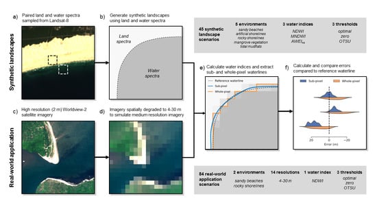
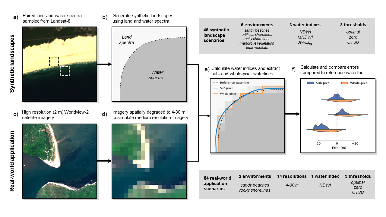
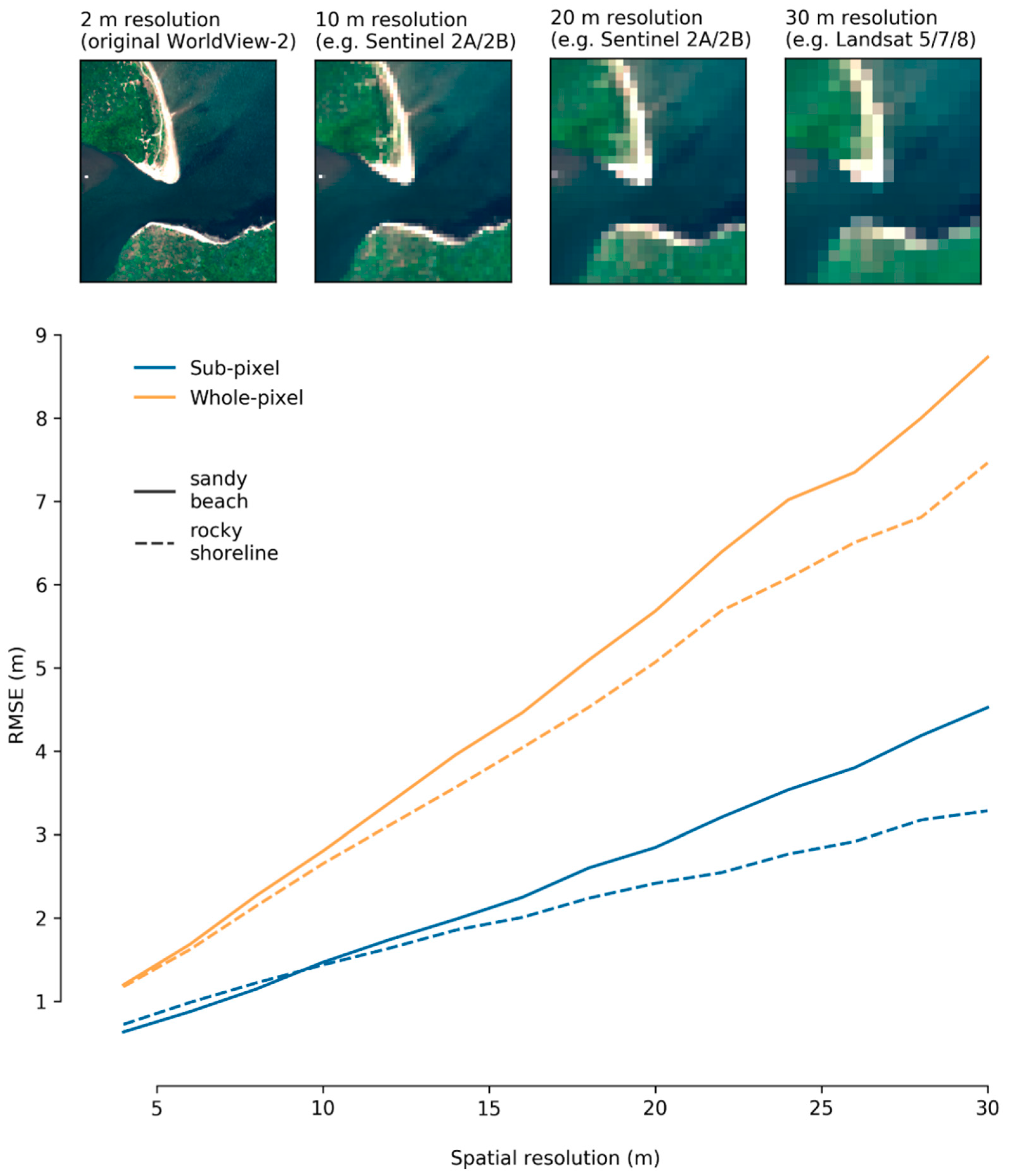
2.1. Influence of Environment on Waterline Extraction Performance

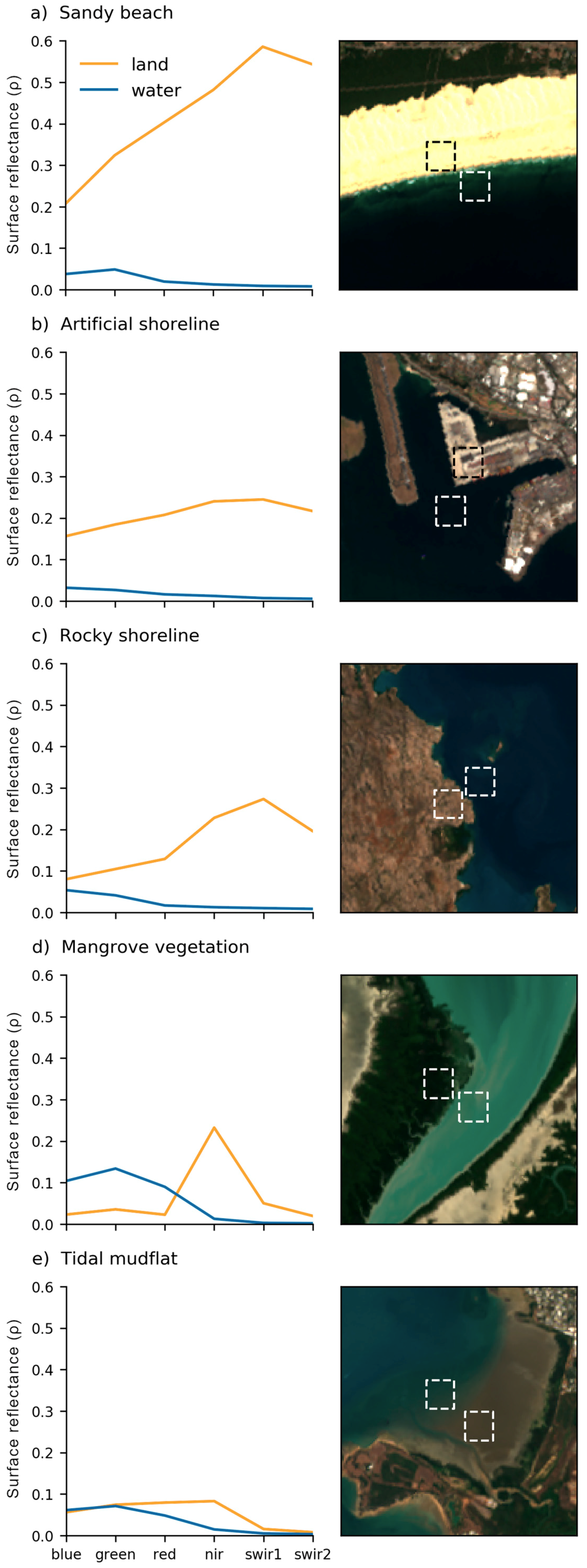
2.1.1. Sample Spectra and Index Calculation

To assess subpixel waterline extraction performance across a range of common land-water boundaries, we extracted a set of typical spectra from freely available Landsat 8 OLI imagery available within the 30 year Digital Earth Australia archive produced by Geoscience Australia [3,4]. This data is available as atmospherically and terrain corrected ‘analysis-ready’ data processed to surface reflectance, allowing reliable spectra to be extracted with no additional processing or calibration required [44]. We focused on five commonly studied environments to explore the influence of contrasting spectral properties on waterline extraction performance: a) sandy beaches [1,6,28,33,34,38,42], b) artificial shorelines [32,45], c) rocky shorelines [10,29,45], d) wetland vegetation [46,47,48], and e) tidal mudflats [7,10,19,49]. Paired samples of land and neighbouring water spectra were extracted from cloud free imagery along the Australian coastline by taking the mean value for each satellite band within each sample region (Figure 2). Imagery acquired at low tide was selected in the case of the tidal mudflat environment. As it would be impractical to analyse the full range of natural spectral variability for any of these individual environments, the sample spectra were intended to serve as a set of spectrally unique examples rather than an exhaustive and representative sample of natural conditions. For each environment, spectral values were assigned to the ‘land’ and ‘water’ pixels of the synthetic landscape to create a multispectral array with six spectral bands (red, green, blue, near-infrared, shortwave infrared 1, shortwave infrared 2) broadly shared by frequently used sources of open-source satellite imagery (e.g., Landsat TM, ETM+, OLI and Sentinel 2 MSI).

Using this array as a high-resolution (i.e., 1.0 m) reference dataset, we then simulated a typical medium resolution satellite dataset (e.g., Landsat) by spatially aggregating the higher-resolution data to a spatial resolution of 30 m using an ‘average’ aggregation rule. This reduced resolution 30 m dataset was then used as the basis for waterline extraction. Initially, we computed a series of common water extraction indices. The normalised difference water index (NDWI, [50]) is one of the most commonly used remote sensing water indices, having been applied to facilitate waterline delineation in a wide range of papers across inland [23,24,26] and coastal environments [7,10,25,51]. This index ranges from -1.0 (land) to 1.0 (water), and uses the ratio of visible green and near-infrared (NIR) reflectance to separate water pixels from land based on water’s high reflectance of visible green light and low reflectance of NIR, and the high reflectance of NIR by dry soil and terrestrial vegetation:

$$NDWI=\frac{\left(Green-NIR\right)}{\left(Green+NIR\right)}$$

(2)

Recently, a modification of the NDWI which substitutes short-wave infrared (SWIR) in place of NIR has seen increasing popularity for waterline extraction [22]. This modified normalised difference water index (MNDWI) has been suggested as a more accurate alternative to NDWI, particularly in environments affected by white water from surf or high levels of turbidity [1,33]. However, this index can produce poor results in intertidal environments where wet substrate remaining after high tide is often mapped as open water [19,20].

$$MNDWI=\frac{\left(Green-SWIR1\right)}{\left(Green+SWIR1\right)}$$

(3)

The automated water extraction index (AWEI) has been proposed to address these limitations of both NDWI and MNDWI. Unlike NDWI and MNDWI, which are based on the relative ratio of green and near-infrared or shortwave radiation, AWEI is based on the sum of multiple spectral bands, and has been shown to produce higher water identification accuracy across a broad range of coastal and inland water environments by maximising spectral contrast between water and land classes [52]. While two formulations of the AWEI have been proposed to deal with extreme shadows in mountainous environments, we focused on the ‘non-shadow’ variant (AWEI_ns) in this study due to the typically low relief of the five environments being assessed:

$$AWE{I}_{ns}=4\times \left(Green-SWIR1\right)-\left(0.25\times NIR+2.75\times SWIR2\right).$$

(4)

2.1.2. Waterline Extraction

We extracted sub-pixel resolution waterlines for each environment and water index using the marching squares with linear interpolation contour extraction algorithm implemented in the Python skimage.measure.find_contour function [53,54]. Contour-based methods aim to detect the boundary between two classes based on a two-dimensional input surface (for example, precisely mapping the position of a given elevation contour from a digital elevation model). When used to extract sub-pixel waterlines from a continuous water index surface, we make the assumption that low or medium resolution pixels along the land-water boundary represent mixed pixels, and that water index values (e.g., NDWI) for these pixels directly reflects the relative proportion of water and land within those pixels. It should therefore be possible to compare the relative water index values of two neighbouring pixels, and use this comparison to more precisely locate the boundary between land and water than simply drawing a line directly along their pixel boundaries. The marching squares with linear interpolation algorithm linearly interpolates between the water index values of neighbouring pixels to map out the precise location of the waterline according to a specified threshold value [53]. For example, where a land pixel has a water index value that is similar to its neighbouring water pixel (indicating the land pixel may contain a significant proportion of water), this will result in the output waterline position being shifted in an inland direction. Theoretically, this allows the location of the derived waterline to be identified at a precision that exceeds the resolution of the input satellite imagery [53].

As waterlines derived from remote sensing water indices can be highly sensitive to the threshold value selected to separate land from water, we extracted subpixel waterlines for three unique thresholds: an ‘optimal’ threshold, a ‘zero’ water index threshold, and an automatically derived threshold. The ‘optimal’ threshold represented the threshold that most closely replicated the high resolution reference shoreline, and was identified for each environment and water index scenario by iterating through a wide range of threshold scenarios (from–1.0 to 1.0 in 0.01 increments for NDWI and MNDWI, and from –2.0 to 2.0 in 0.01 increments for AWEI_ns given its larger range of possible values), and selecting the water index that produced the lowest RMSE compared to the high resolution reference waterline. This threshold scenario was intended to compare the best-possible waterline extraction performance in an application where the ideal water index threshold was known. As knowing the ideal threshold ahead of an analysis is often not possible, the ‘zero’ water index threshold scenario used a constant zero threshold to extract waterlines, a procedure which is commonly used in operational waterline extraction applications conducted across large spatial extents [7,10]. Finally, procedures for automatically deriving threshold values based on the histogram distribution of water index values have been increasingly used to provide improved waterline extraction performance in complex heterogeneous environments where a single threshold (i.e., 0) would produce poor results [6,39,42]. We used Otsu thresholding implemented by the Python function skimage.filters.threshold_otsu to calculate an automatic threshold for each environment and water index [54,55]. This image processing approach identifies a threshold value that best separates a histogram of water index values into two distinct classes (e.g., water and land, [55]).

Subpixel shorelines extracted for each environment, water index and threshold scenario were converted to vector line features to facilitate comparisons against the 1.0 m high-resolution reference waterline. To provide a comparison dataset against which to compare the accuracy and precision of sub-pixel resolution waterlines, we additionally extracted matching waterlines for each scenario using a traditional whole-pixel thresholding approach (henceforth, ‘whole-pixel’ waterlines). This involved identifying all pixels with a water index equal to or above the given threshold as ‘water’ pixels and all values less than the threshold as ‘land’ pixels. This thresholded dataset was then polygonised, and a vector line feature extracted along the boundary of the two classes.

2.1.3. Statistical Comparison

We evaluated the ability of our two extracted waterlines to reproduce the true waterline position by computing distances (errors) between the 1.0 m high-resolution reference waterline and each set of sub-pixel and whole-pixel waterlines. At 1.0 m intervals along the reference waterline, we calculated Euclidean distance to the nearest point on both the sub-pixel and whole-pixel waterlines using the distance method from the shapely Python package [56]. Distances were assigned a direction (water- or land-ward offset from the reference waterline) based on whether the comparison point fell in a ‘land’ or ‘water’ pixel in the synthetic landscape: if the comparison point fell in a ‘land’ pixel, this distance was assigned a negative value to infer a land-ward offset. These distance errors were calculated for each environment, water index and threshold scenario, and compared using split violin plots to visualize error distributions between the sub-pixel and whole-pixel water extraction approaches. We additionally calculated two summary statistics to evaluate the extracted waterlines: root mean square error (RMSE) assessed the absolute accuracy of the derived waterlines compared to the reference waterline, while standard deviation allowed us to compare overall precision, or how closely the extracted waterlines replicated the overall shape of the reference shoreline even if the lines were consistently offset in a water or land-ward direction (e.g., a shoreline that closely followed the relative shape of the reference shoreline would have a low variability in error values).

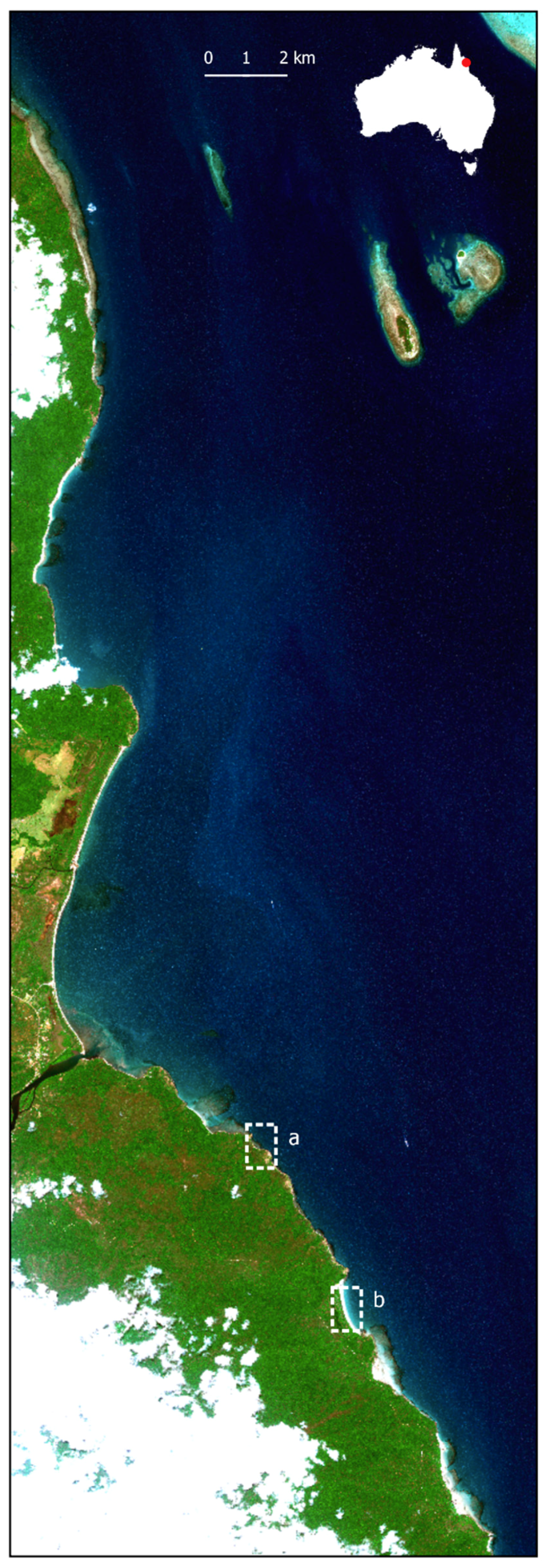
2.2. Real-World Application Using WorldView-2

Although the synthetic data-based modelling framework above allowed us to rapidly test and isolate the performance of sub-pixel waterline extraction across a wide range of environmental and image processing scenarios, the theoretical approach represented a significant simplification of the complex heterogeneous environments typically found in satellite imagery. To complement the theoretical analysis, we assessed sub-pixel waterline extraction using high resolution satellite imagery. We obtained a largely cloud-free 2.0 m resolution WorldView-2 (WV-2) image (acquired 13^th November 2010, 00:40 UTC) for a complex coastal region in north-western Queensland that contained extensive sandy beaches and rocky shoreline environments (Figure 3). This six band multispectral image (red, green, blue, yellow, near infrared 1, near infrared 2) was processed to surface reflectance using a bidirectional reflectance distribution function (BRDF) and topographically corrected MODTRAN-based atmospheric correction as detailed in Li et al. [44]. As WV-2 lacks the shortwave infrared bands required to compute MNDWI and AWEI_ns, we focused on NDWI (using the NIR 1 band) as the water index used to extract waterlines.

To provide a high-resolution reference shoreline, we extracted a vector shoreline at the imagery’s native 2.0 m resolution based on a consistent zero NDWI threshold. While this consistent threshold did not account for the different coastal environments present in the image, using a consistent threshold allowed us to provide a single point-of-truth within the modelling framework that could be compared consistently against lower resolution shorelines, and eliminated any subjectivity associated with manually digitising shorelines. This reference waterline was stratified into sandy beaches and rocky shorelines by visually inspecting the underlying true colour WV-2 imagery, allowing us to compare results across different coastal environments.

To eliminate the confounding influence of tidal processes and coastal change between image acquisitions, we simulated lower resolution satellite imagery using spatially degraded versions of the WV-2 image itself rather than obtain co-incident imagery from other satellite platforms (e.g., Landsat or Sentinel 2). We progressively spatially degraded the 2.0 m resolution WV-2 image from 4 m to 30 m (in 2 m increments) using the average aggregation rule applied in the theoretical approach. Each aggregated image was used to compute NDWI, and extract sub-pixel and whole-pixel waterlines for the optimal, zero and automated Otsu index threshold scenarios above. Otsu thresholding was conducted separately on the two coastal environments (sandy beaches and rocky shorelines) by first buffering the reference shoreline by 50 m, and using this polygon as a mask to ensure that water and land classes were equally represented in the NDWI layer (an assumption of the Otsu process). Waterlines for each scenario were then statistically compared against the reference waterline by computing Euclidean distance errors at 1 m intervals along the extracted waterlines, and assessing RMSE and standard deviation error across the range of spatial resolutions for each of the two coastal environments.

All analyses in this study were conducted on Australia’s National Computing Infrastructure’s Virtual Desktop infrastructure (8 vCPUs, 32GB RAM). Code was written in the Python 3.6 programming language based on open-source functions from the OpenDataCube (https://www.opendatacube.org/), xarray [57], NumPy [58], SciPy [59], scikit-image [54] and pandas [60] libraries. All figures were generated using xarray, Matplotlib [61] and seaborn [62] data visualization libraries.

To allow the analyses presented here to be applied to future studies, functions for rapidly extracting waterlines from large multi-dimensional satellite data arrays are provided as an open-source toolset (Supplementary Materials).

3. Results and Discussion

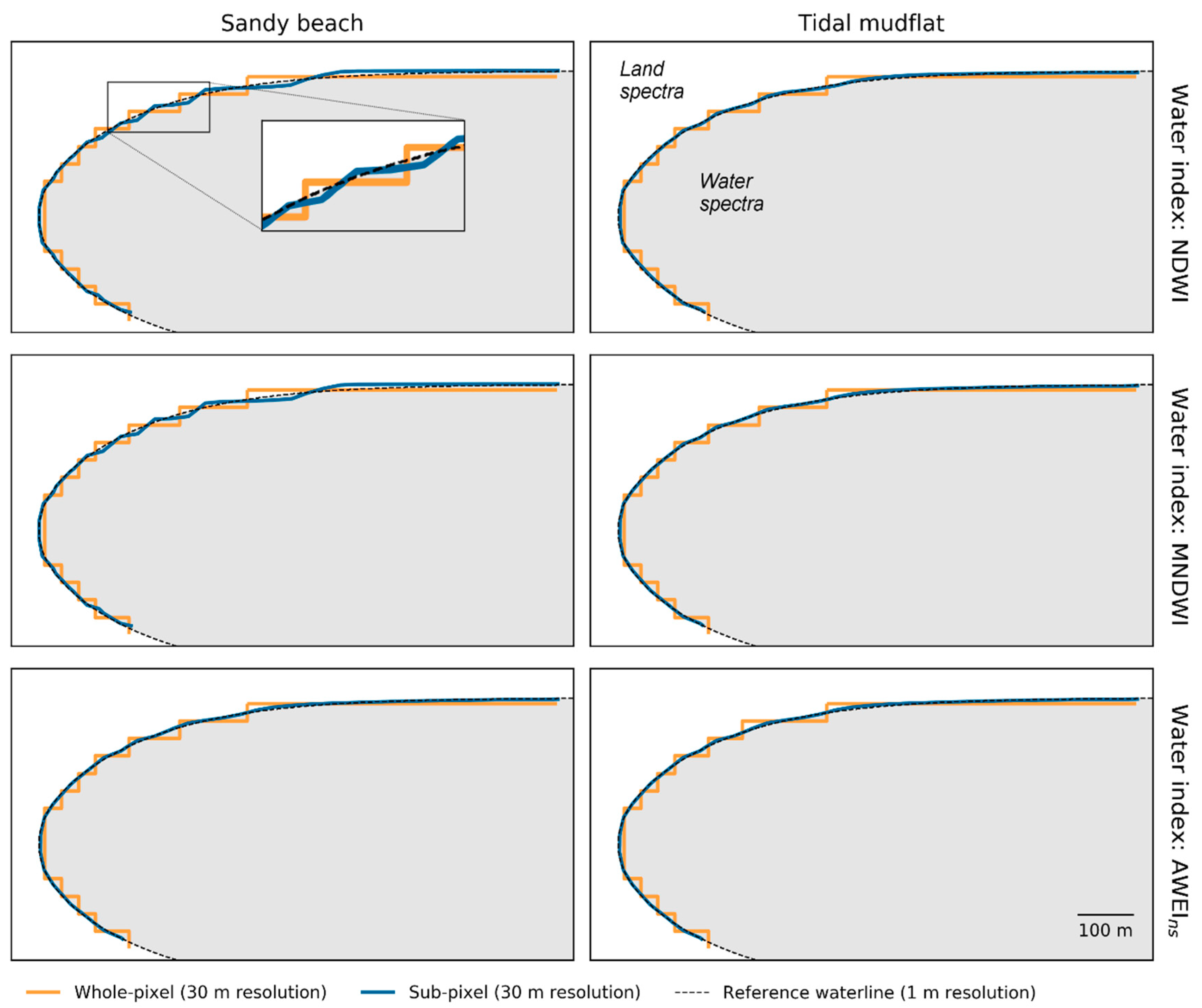
3.1. Sub-Pixel Waterline Extraction Performance

We evaluated waterline extraction performance based on our synthetic landscape approach by comparing the distribution of distances in metres from the modelled to the reference shoreline (errors), using root mean squared error (RMSE) to evaluate whether errors were tightly distributed around 0 (Figure 4). Across 38 of our 45 synthetic landscape scenarios, RMSE for sub-pixel waterline extraction was lower compared to the whole-pixel approach, a clear result that indicated the method was able to more accurately represent the reference waterline position. This was particularly true for ‘optimal’ threshold scenarios, where sub-pixel waterlines were between 2.1 to 5.8 times more accurate than equivalent whole-pixel waterlines across all landscapes and water indexes (

Table 1. Root mean squared error (RMSE in metre units) and standard deviation (in metre units) of errors compared to the reference waterline for sub-pixel and whole-pixel waterline extraction approaches across five sample environments with contrasting spectral characteristics. Waterline extraction methods were compared using three water indices (normalised difference water index (NDWI), modified normalised difference water index (MNDWI), and automated water extraction index ‘non-shadow’ variant (AWEI_ns)) and thresholding strategies (optimal thresholding, zero thresholding and automated Otsu thresholding). Bold cells in the RMSE and standard deviation columns indicate the best modelling performance for each scenario (i.e., sub-pixel or whole-pixel waterlines).

			RMSE (m)		Standard Deviation (m)
Spectra	Water Index	Threshold	Sub-pixel	Whole-pixel	Sub-pixel	Whole-pixel
Sandy beach	NDWI	Optimal	3.74	8.63	3.73	7.60
		Zero	4.17	12.85	3.87	8.35
		Otsu	10.07	14.93	4.31	8.39
	MDWI	Optimal	3.99	8.63	3.97	7.60
		Zero	5.53	14.93	4.21	8.39
		Otsu	9.40	16.24	4.48	8.80
	AWEIns	Optimal	1.50	8.63	1.50	7.59
		Zero	21.60	16.94	4.37	8.94
		Otsu	1.58	8.63	1.49	7.60
Artificial shoreline	NDWI	Optimal	3.48	8.63	3.39	7.60
		Zero	3.89	12.85	3.61	8.35
		Otsu	5.63	14.93	3.77	8.39
	MDWI	Optimal	3.68	8.63	3.65	7.60
		Zero	3.68	9.58	3.65	8.03
		Otsu	10.32	14.93	4.28	8.39
	AWEIns	Optimal	1.51	8.63	1.51	7.59
		Zero	20.39	16.24	4.06	8.80
		Otsu	1.53	8.70	1.50	8.27
Rocky shoreline	NDWI	Optimal	2.73	8.63	2.72	7.60
		Zero	5.64	12.85	2.98	8.35
		Otsu	7.67	14.93	3.14	8.39
	MDWI	Optimal	2.93	8.63	2.93	7.60
		Zero	6.72	14.43	3.29	8.22
		Otsu	7.01	14.93	3.32	8.39
	AWEIns	Optimal	1.50	8.63	1.51	7.59
		Zero	19.79	16.24	3.90	8.80
		Otsu	1.57	8.63	1.49	7.60
Wetland vegetation	NDWI	Optimal	1.75	8.63	1.74	7.59
		Zero	3.06	8.98	1.67	7.70
		Otsu	4.04	8.98	1.71	7.70
	MDWI	Optimal	1.52	8.63	1.52	7.59
		Zero	18.45	13.41	4.32	8.42
		Otsu	2.08	9.04	1.62	9.04
	AWEIns	Optimal	1.51	8.63	1.51	7.59
		Zero	9.02	10.05	2.04	8.85
		Otsu	1.56	8.70	1.49	8.27
Tidal mudflat	NDWI	Optimal	1.75	8.63	1.74	7.59
		Zero	17.68	13.23	3.76	8.60
		Otsu	4.32	9.58	1.73	8.03
	MDWI	Optimal	1.55	8.63	1.55	7.60
		Otsu	2.22	8.98	1.53	7.70
	AWEIns	Optimal	1.51	8.70	1.51	8.27
		Otsu	1.51	8.70	1.51	8.27

, Figure 4). Sub-pixel waterline accuracy was the highest using the AWEI_ns index, where all waterlines extracted from the 30 m resolution data using ‘optimal’ thresholds had an RMSE of 1.50–1.51 m (Table 1, Figure 4). All seven scenarios where sub-pixel waterlines had higher RMSE than whole-pixel waterlines occurred using ‘zero’ thresholding (see Section 3.3, Effect of Water Index Threshold below).

Calculating RMSE allowed us to compare waterline extraction accuracy in absolute terms. However, many applications of waterline extraction such as coastal erosion and inland water level monitoring require an ability to monitor the relative location or shape of the shoreline consistently across time. To quantify how precisely waterline extraction approaches could reproduce the shape of the waterline, we calculated the standard deviation of errors between the modelled and reference waterline, assuming that a low variance in errors indicated that modelled shorelines were always positioned a consistent distance away from the true shoreline position. In all 45 scenarios, sub-pixel waterline errors exhibited significantly lower variance compared to whole-pixel waterlines, indicating a far better reproduction of waterline shape at a scale of less than one pixel (Table 1, Figure 4). Although this result was most pronounced across ‘optimal’ threshold scenarios where standard deviations were up to 5.5 times lower than whole-pixel waterlines, lower variances (i.e., 1.9 to 4.6 times lower) were also found across all ‘zero’ threshold scenarios (Table 1, Figure 4). This was the case even when sub-pixel waterlines had higher RMSE due to being clearly offset from the reference waterline position. Importantly, this result suggests that the resulting sub-pixel waterlines are likely to better reflect the relative waterline shape, even when offset land or sea-ward from the true waterline position due to an inappropriate choice of water index threshold. This result indicates that even a zero threshold approach based on a non-optimal water index threshold combined with sub-pixel waterline extraction can be suitable for applications where the priority is consistently monitoring trends in relative water line positions through time. As we illustrate in the following sections, selecting the appropriate thresholds and indexes both spatially and temporally to enable like-for-like comparison is a non-trivial exercise.

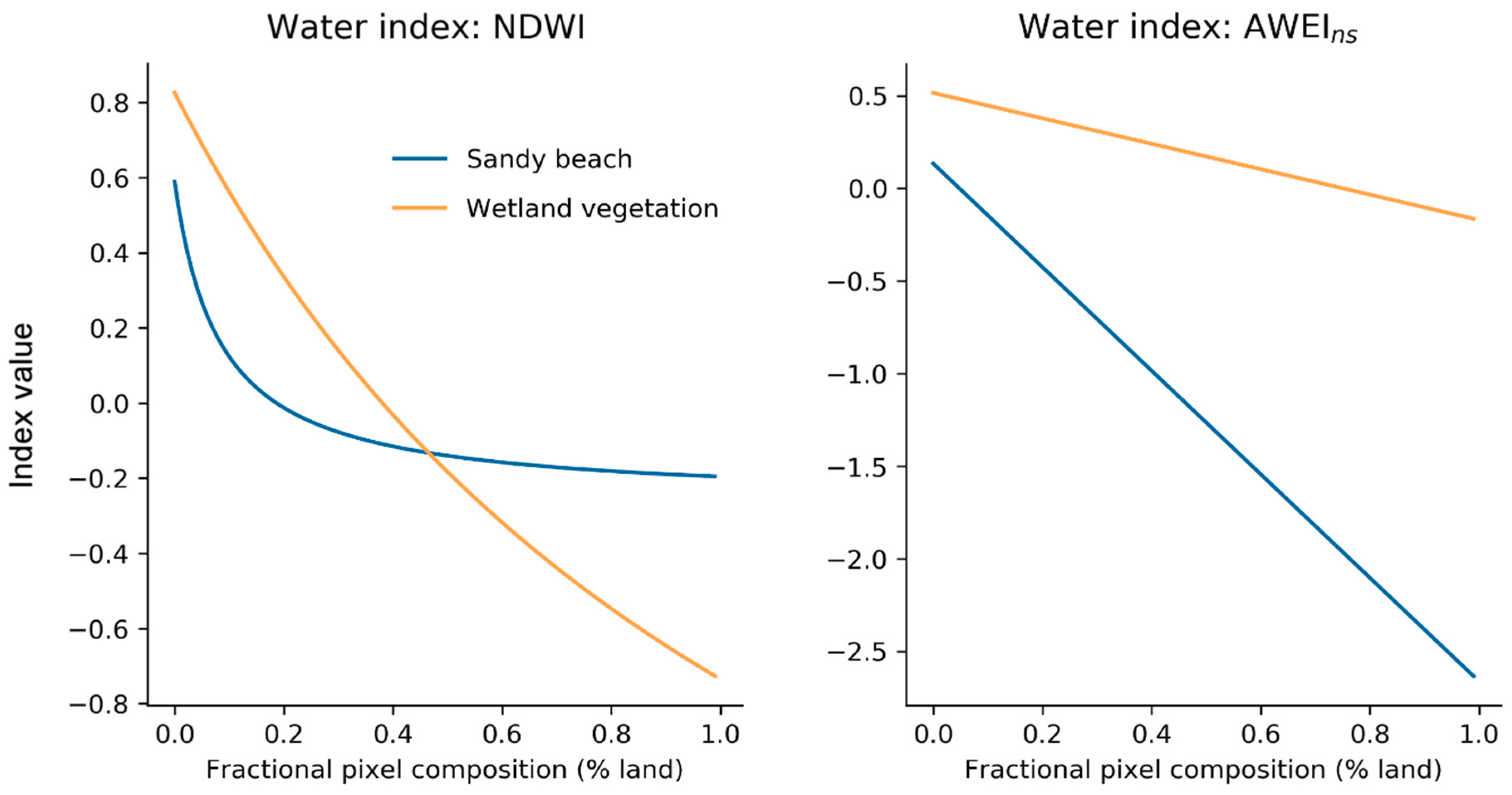
3.2. Effect of Spectra and Water Index

While sub-pixel waterlines more accurately and precisely reproduced reference waterline position and shape across the majority of our scenarios, we observed key differences by environment type which have important implications for remote sensing-based waterline extraction. ‘Optimal’ threshold results for our two normalised difference water indices (NDWI and MNDWI) showed a consistent trend of decreasing RMSE and standard deviation which coincided with a decrease in spectral contrast between water and land features (e.g., lower accuracy and precision along high contrast artificial shorelines and sandy beaches, and better accuracy and precision in low contrast tidal mudflats and wetland vegetation; Figure 4). For example, sub-pixel RMSE and standard deviation for NDWI waterlines improved from 3.74 and 3.73 m in sandy beach environments to 1.75 and 1.74 in tidal mudflats (Table 1). This effect could be qualitatively observed by comparing the shape of the shorelines generated for sandy beach and tidal mudflat environments (Figure 5). In tidal mudflats environments with low spectral contrast between wet mud and turbid water, sub-pixel waterlines closely follow the true shape of the reference shoreline along the entire length of the synthetic coastline. In comparison, sub-pixel waterlines in sandy beach environments displayed repeated undulating artefacts along the shallower curved region of the landscape (Figure 5). In these environments, high contrast between bright sand and dark water reduced the ability of the sub-pixel waterline extraction to resolve fine-scale curves or subtle undulations in waterline shape.

Although spectral contrast appeared to negatively affect both NDWI and MNDWI, the AWEI_ns index did not reveal any relationship with spectral contrast. Accuracy and precision for AWEI_ns remained relatively constant across all environments (Table 1, Figure 4), with no obvious step-like artefacts visible in the resulting waterlines (Figure 5). An explanation for this effect can be found in the non-linear response of certain water index values to the sub-pixel fractional coverage of water within each pixel. In environments with bright land features and dark water, a small increase in the proportion of land within a pixel can produce a large change in remote sensing indices like NDWI that are based on the ratio of visible and infrared radiation. To visualise this, we can calculate an NDWI value based on the weighted average spectra for each satellite band as the percentage of land within the pixel increases from 0 to 100% (Figure 6). In a low contrast environment such as a tidal flat, NDWI values decrease approximately linearly with increasing land. However, in a high contrast sandy beach environment, even a small increase in land coverage (e.g., from 0% to 10%) can result in a rapid decrease in NDWI. When used as the input for sub-pixel waterline extraction, this response drives the repeated undulating response of the waterline, with the resulting waterline position highly affected by a small change in the fractional coverage of bright sand. In contrast, the AWEI_ns index is based on the sum of six spectral bands and linear coefficients, and responds linearly to increasing proportion of land or water within a pixel (Figure 6).

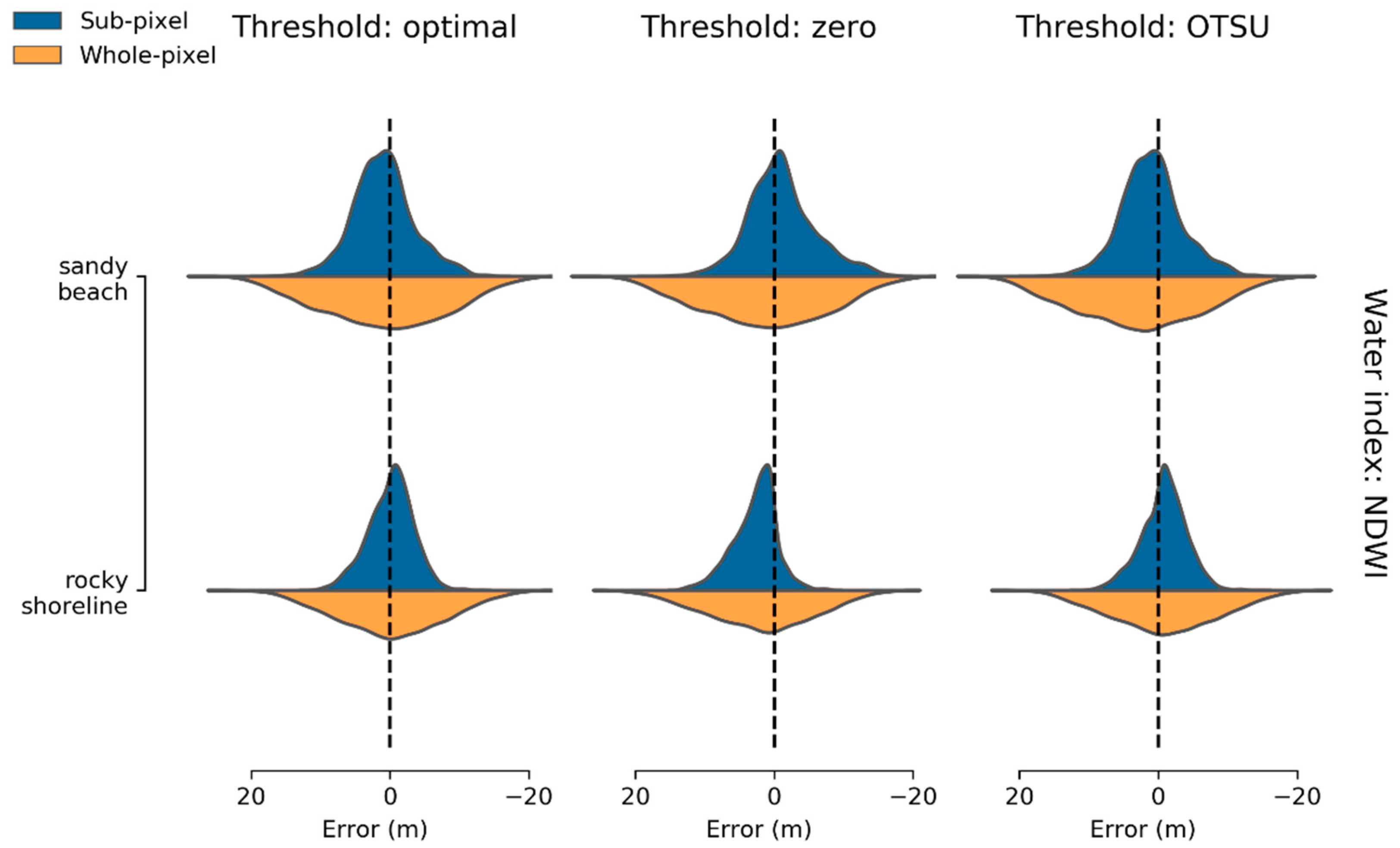
3.3. Effect of Water Index Threshold

The ‘optimal’ water index threshold scenarios allowed us to assess the theoretical limits of sub-pixel waterline extraction performance under ideal conditions where the value of the best threshold value was known. However, threshold selection remains one of the key limitations of satellite-derived waterline extraction, particularly where reference data is not available to tailor the threshold to contrasting heterogeneous coastal or inland water environments [1,63]. This is frequently the case for operation analyses aimed at modelling waterlines across large spatial extents (e.g., at regional, continental or global scale). To evaluate how sub-pixel waterline extraction performs when the optimal value of the threshold is not known in advance, we also compared performance using two more realistic threshold selection strategies. The simplest ‘zero’ threshold scenario applied a consistent threshold of zero to all environments and metrics, in an approach which has been widely used in waterline extraction analyses [7,22,64]. Our results indicate a uniform zero threshold was unable to consistently reproduce the absolute reference waterline position across the five contrasting environments or three water indices we assessed. In an extreme example, a ‘zero’ threshold for tidal mudflat environments completely failed to differentiate between land and water for both the MNDWI and AWEI_ns indices due to the spectral similarity of wet substrate with turbid water in the short-wave infrared satellite bands that were utilised by both indices ([19,20], Figure 4). Although poor modelling performance was observed using the ‘zero’ threshold for both sub- and whole-pixel waterlines, the narrower distribution of sub-pixel waterline errors meant that this method was more sensitive to poor threshold selection compared to whole-pixel waterlines whose larger error distribution typically overlapped with the true location of the waterline (Table 1, Figure 4).

To address the limitations of a consistent zero threshold, we assessed model performance using water index thresholds optimised using Otsu’s method. Otsu has been proposed as an automated method for deriving locally-tuned threshold values for operational waterline analyses, however, the performance of the approach on sub-pixel waterline accuracy has not previously been assessed. Our results indicate that ‘Otsu’ thresholding significantly improved the consistency of waterlines extracted using the sub-pixel approach, leading to error distributions which were generally narrower than corresponding zero threshold distributions, and more comparable across different environment types (Figure 4). This was particularly the case for wetland vegetation and tidal mudflat environments, which saw improvements in overall RMSE of up to 16.4 m between ‘zero’ and ‘Otsu’ scenarios (e.g., wetland vegetation MNDWI; Table 1, Figure 4). Although Otsu typically did not reproduce the absolute or relative accuracy of ‘optimal’ thresholds, the improvement in results compared to zero threshold scenarios results indicates that automated threshold selection can complement sub-pixel waterline extraction approaches. This is likely to be particularly significant in large-scale analyses covering diverse environment types, where the influence of inappropriate threshold selection may overwhelm increases in accuracy gained from implementing sub-pixel waterline extraction methods.

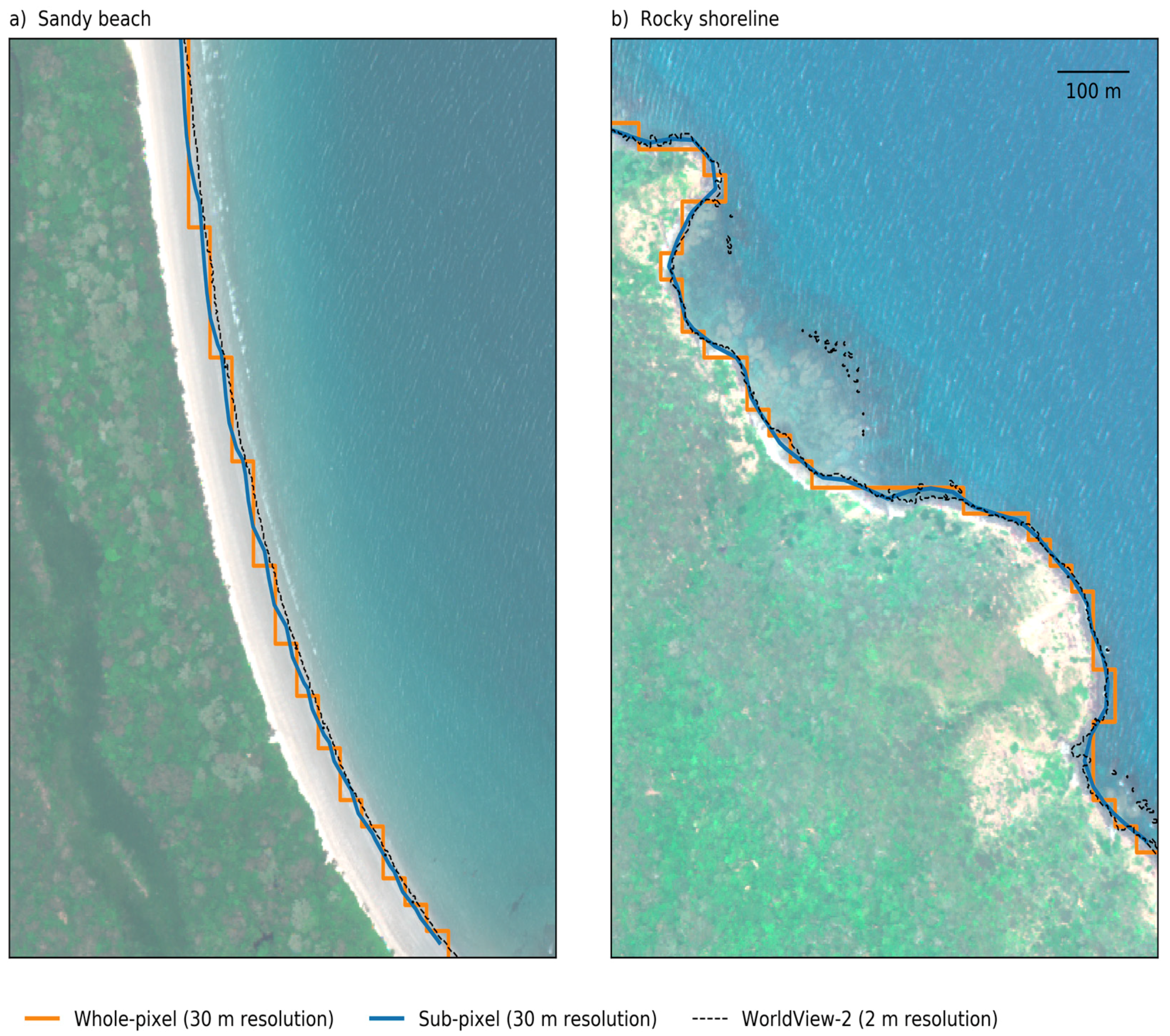
3.4. Real-World Application

By progressively spatially degrading high resolution (2 m) WorldView-2 remote sensing imagery, it was possible to simulate lower resolution satellite imagery and assess the impact of spatial resolution on waterline extraction performance in a more complex real-world scenario. At 30 m resolution (equivalent to Landsat TM, ETM+ and OLI bands), sub-pixel waterlines were 1.9 to 2.3 times more accurate than whole-pixel waterlines both in absolute terms (e.g., RMSE of 3.28–4.52 m compared to 7.46–8.73 m for whole-pixel waterlines), and in their ability to reproduce the relative shape of the reference coastline (e.g., standard deviation of 3.27–4.42 m compared to 7.46–8.70 m;

Table 2. Root mean squared error (RMSE in metre units) and standard deviation (in metre units) of sub-pixel and whole-pixel waterline extraction errors compared to the 2 m resolution WorldView-2 reference waterline. Results are shown for optimal NDWI thresholds for two coastal environments (rocky shorelines and sandy beaches) and four key resolutions (4 m as relevant to Planet Labs 3 m PlanetScope and 5 m RapidEye imagery, 10 m and 20 m as equivalent to Sentinel 2 MSI, and 30 m as equivalent to Landsat TM, ETM+, and OLI). Bold cells for the RMSE and standard deviation columns indicate the best modelling performance for each scenario (i.e., sub-pixel or whole-pixel waterlines). For ‘zero’ and ‘Otsu’ threshold results, refer to Appendix A.

		RMSE (m)		Standard Deviation (m)
Environment	Spatial Resolution (m)	Sub-pixel	Whole-pixel	Sub-pixel	Whole-pixel
Rocky shoreline	4	0.72	1.17	0.72	1.15
Rocky shoreline	10	1.43	2.65	1.43	2.65
Rocky shoreline	20	2.41	5.07	2.41	5.07
Rocky shoreline	30	3.28	7.46	3.27	7.46
Sandy beach	4	0.63	1.19	0.63	1.17
Sandy beach	10	1.47	2.80	1.47	2.79
Sandy beach	20	2.84	5.68	2.84	5.67
Sandy beach	30	4.52	8.73	4.42	8.70

, Figure 7). The ability of the sub-pixel approach to accurately reproduce the true waterline even at this relatively coarse resolution can be qualitatively observed in Figure 8a, where sub-pixel waterlines (blue) closely follow small undulations in the path of the dashed 2 m high resolution waterline which are considerably smaller in scale than the pixel resolution captured by the equivalent whole-pixel waterlines.

Sub-pixel accuracy increased approximately linearly with increasing resolution, with subpixel shorelines achieving accuracies of up to 2.41 m at 20 m Sentinel 2 resolution equivalent, and 1.43 m at 10 m Sentinel 2 resolution (Figure 9). Waterlines based on the original 2 m Worldview-2 dataset (8515 by 21352 pixels) were extracted in 3.98 seconds (± 115 ms for ten repetitions) for 143 km of coastline on Australia’s National Computing Infrastructure’s Virtual Desktop infrastructure (8 vCPUs, 32GB RAM). Waterline extractions at 30 m Landsat resolution took 1.93 seconds (± 116 ms) at a rate of 0.013 seconds per kilometer of coastline. This is equivalent to 13 minutes to process the entire ~60,000 km coastline of Australia (the eighth longest coastline in the world), which is considered suitable for large-scale operational analysis. Our results demonstrate that sub-pixel waterlines can be reliably and efficiently extracted across complex heterogeneous coastal environments, and achieve accuracies that consistently exceed the accuracy of traditional waterline extraction approaches regardless of the spatial scale of analysis.

Comparing two unique coastal environments (sandy beaches and rocky shorelines) allowed us to assess whether we could reproduce the effects of spectral contrast on waterline accuracy that we observed in the simulated landscape analysis. Although the effect was more subtle than in the simulated analysis, Figure 9 highlights that RMSE accuracies for the sandy beach waterlines were routinely lower than rocky shorelines, particularly at coarser resolutions (e.g., 30 m pixels). A qualitative inspection of the resulting shorelines for these two environments revealed that high contrast white sandy beaches were associated with similar repeated undulating artefacts (Figure 8a). While previous studies have shown a relationship between spectral contrast and absolute waterline offsets (e.g., brighter land spectra leading to a land-ward bias in waterline errors, [32]), our results indicate that caution should be used when applying waterline extraction approaches to water indices such as NDWI or MNDWI which react non-linearly to underlying distributions of water and land. This is particularly significant given the majority of waterline extraction analyses to date have focused on analysing sandy beach environments which are likely to be most vulnerable to contrast-driven modelling artefacts. While the limited selection of available WorldView-2 bands prevented us from assessing model performance using an alternative index such as AWEI_ns, we recommend that future studies evaluate model performance using water indices that respond linearly to the fractional coverage of land and water. Alternatively, sub-pixel waterline extraction could be applied directly to more physically meaningful water index surfaces, such as per-pixel estimates of fractional water coverage derived from spectral unmixing analysis [65,66,67]. This will ensure that sub-pixel resolution waterline positions can be compared reliably across environments with unique and contrasting spectral characteristics.

4. Conclusions

In this study, we have evaluated a sub-pixel waterline extraction method that shows a strong ability to reproduce both absolute waterline positions and relative shape at a resolution that far exceeds that of traditional whole-pixel thresholding methods, particularly in environments without extreme contrast between water and land. Given the low computational overhead and open source availability of the technique, the approach is likely to be suitable for large-scale waterline extraction analyses as an easy-to-implement substitute for less precise whole-pixel approaches.

Although sub-pixel waterline extraction provides key advantages over whole-pixel approaches, the extra sensitivity of the method makes it vulnerable to two key challenges facing remote sensing-based waterline extraction in general: the selection and thresholding of a reliable water index [1]. Our results indicate that although zero threshold approaches were unable to consistently reproduce absolute waterline positions, sub-pixel waterlines based on a zero threshold were better able to model relative waterline shape compared to whole-pixel waterlines. Simple zero threshold approaches to mapping surface water are therefore likely to be enhanced through integration with sub-pixel waterline delineation, particularly when the application requires the consistent monitoring of relative water line positions through time.

Where absolute accuracy is the priority, our results show that automated index thresholding approaches (e.g., Otsu) can be combined with sub-pixel methods to extract waterlines that approach the accuracy of optimal thresholds. However, while automated thresholding methods may work successfully for small study areas and discrete time-steps, producing seamless and consistent waterline datasets through time and across complex heterogeneous environments remains a challenge. There is a critical need for the development of new continuous along-shore methods for determining thresholds [68,69] and approaches for ensuring the temporal consistency of automated thresholds to support optimising and operationalising the mapping of dynamic waterlines across space and time. Finally, our results also highlight the importance of selecting remote sensing indices which respond linearly to changes in underlying proportions of water and land, and suggest that future work should focus on integrating the technique with more physically meaningful water indices which directly quantify the proportion of water within each pixel.

To support future applications of the approach, we have provided the tools used to extract sub-pixel waterlines as open-source code (Supplementary Materials). These functions can be applied directly to large multi-dimensional satellite datasets, making them suitable for applying to large scale remote sensing workflows such as those enabled by Open Data Cube [3,4] or Google Earth Engine [5]. By enabling the automatic extraction of sub-pixel waterlines consistently across space and time, it is anticipated that these tools may supplement existing open source coastal monitoring software [70] and assist in scaling up current local-scale waterline analyses to provide insights into drivers of environmental change operating at regional, continental or global scales. Future work will focus on applying sub-pixel waterline extraction methods to provide accurate estimates of waterbody area and volume for inland reservoirs and lakes to monitor the impact of drought and water extraction within semi-arid inland Australia, and operationalising the approach to monitor fine-scale erosion and coastal change across complex coastal environments along the entire Australian coastline.

References

1. Kelly, J.T.; Gontz, A.M. Using GPS-surveyed intertidal zones to determine the validity of shorelines automatically mapped by Landsat water indices. Int. J. Appl. Earth Obs. Geoinf. 2018, 65, 92–104. [Google Scholar] [CrossRef]
2. Kopp, S.; Becker, P.; Doshi, A.; Wright, D.J.; Zhang, K.; Xu, H. Achieving the Full Vision of Earth Observation Data Cubes. Data 2019, 4, 94. [Google Scholar] [CrossRef] [Green Version]
3. Dhu, T.; Dunn, B.; Lewis, B.; Lymburner, L.; Mueller, N.; Telfer, E.; Lewis, A.; McIntyre, A.; Minchin, S.; Phillips, C. Digital earth Australia—Unlocking new value from earth observation data. Big Earth Data 2017, 1, 64–74. [Google Scholar] [CrossRef] [Green Version]
4. Lewis, A.; Oliver, S.; Lymburner, L.; Evans, B.; Wyborn, L.; Mueller, N.; Raevksi, G.; Hooke, J.; Woodcock, R.; Sixsmith, J.; et al. The Australian Geoscience Data Cube—Foundations and lessons learned. Remote Sens. Environ. 2017, 202, 276–292. [Google Scholar] [CrossRef]
5. Gorelick, N.; Hancher, M.; Dixon, M.; Ilyushchenko, S.; Thau, D.; Moore, R. Google Earth Engine: Planetary-scale geospatial analysis for everyone. Remote Sens. Environ. 2017, 202, 18–27. [Google Scholar] [CrossRef]
6. Luijendijk, A.; Hagenaars, G.; Ranasinghe, R.; Baart, F.; Donchyts, G.; Aarninkhof, S. The state of the world’s beaches. Sci. Rep. 2018, 8, 6641. [Google Scholar] [CrossRef]
7. Sagar, S.; Roberts, D.; Bala, B.; Lymburner, L. Extracting the intertidal extent and topography of the Australian coastline from a 28 year time series of Landsat observations. Remote Sens. Environ. 2017, 195, 153–169. [Google Scholar] [CrossRef]
8. Murray, N.J.; Phinn, S.R.; DeWitt, M.; Ferrari, R.; Johnston, R.; Lyons, M.B.; Clinton, N.; Thau, D.; Fuller, R.A. The global distribution and trajectory of tidal flats. Nature 2019, 565, 222–225. [Google Scholar] [CrossRef]
9. Lymburner, L.; Bunting, P.; Lucas, R.; Scarth, P.; Alam, I.; Phillips, C.; Ticehurst, C.; Held, A. Mapping the multi-decadal mangrove dynamics of the Australian coastline. Remote Sens. Environ. 2019. [Google Scholar] [CrossRef]
10. Bishop-Taylor, R.; Sagar, S.; Lymburner, L.; Beaman, R.J. Between the tides: Modelling the elevation of Australia’s exposed intertidal zone at continental scale. Estuar. Coast. Shelf Sci. 2019, 23, 115–128. [Google Scholar] [CrossRef]
11. Mueller, N.; Lewis, A.; Roberts, D.; Ring, S.; Melrose, R.; Sixsmith, J.; Lymburner, L.; McIntyre, A.; Tan, P.; Curnow, S.; et al. Water observations from space: Mapping surface water from 25 years of Landsat imagery across Australia. Remote Sens. Environ. 2016, 174, 341–352. [Google Scholar] [CrossRef] [Green Version]
12. Pekel, J.-F.; Cottam, A.; Gorelick, N.; Belward, A.S. High-resolution mapping of global surface water and its long-term changes. Nature 2016, 540, 418. [Google Scholar] [CrossRef]
13. Vousdoukas, M.I.; Almeida, L.P.M.; Ferreira, Ó. Beach erosion and recovery during consecutive storms at a steep-sloping, meso-tidal beach. Earth Surf. Process. Landf. 2012, 37, 583–593. [Google Scholar] [CrossRef]
14. Long, N.; Millescamps, B.; Guillot, B.; Pouget, F.; Bertin, X. Monitoring the Topography of a Dynamic Tidal Inlet Using UAV Imagery. Remote Sens. 2016, 8, 387. [Google Scholar] [CrossRef] [Green Version]
15. Almeida, L.P.; Almar, R.; Bergsma, E.W.J.; Berthier, E.; Baptista, P.; Garel, E.; Dada, O.A.; Alves, B. Deriving High Spatial-Resolution Coastal Topography From Sub-meter Satellite Stereo Imagery. Remote Sens. 2019, 11, 590. [Google Scholar] [CrossRef] [Green Version]
16. Ogilvie, A.; Belaud, G.; Massuel, S.; Mulligan, M.; Le Goulven, P.; Calvez, R. Surface water monitoring in small water bodies: potential and limits of multi-sensor Landsat time series. Hydrol. Earth Syst. Sci. 2018, 22, 4349. [Google Scholar] [CrossRef] [Green Version]
17. Pereira, B.; Medeiros, P.; Francke, T.; Ramalho, G.; Foerster, S.; Araújo, J.C.D. Assessment of the geometry and volumes of small surface water reservoirs by remote sensing in a semi-arid region with high reservoir density. Hydrol. Sci. J. 2019, 64, 66–79. [Google Scholar] [CrossRef]
18. Tulbure, M.G.; Broich, M.; Stehman, S.V.; Kommareddy, A. Surface water extent dynamics from three decades of seasonally continuous Landsat time series at subcontinental scale in a semi-arid region. Remote Sens. Environ. 2016, 178, 142–157. [Google Scholar] [CrossRef]
19. Ryu, J.-H.; Won, J.-S.; Min, K.D. Waterline extraction from Landsat TM data in a tidal flat: A case study in Gomso Bay, Korea. Remote Sens. Environ. 2002, 83, 442–456. [Google Scholar] [CrossRef]
20. Ryu, J.-H.; Kim, C.-H.; Lee, Y.-K.; Won, J.-S.; Chun, S.-S.; Lee, S. Detecting the intertidal morphologic change using satellite data. Estuar. Coast. Shelf Sci. 2008, 78, 623–632. [Google Scholar] [CrossRef]
21. Park, W.; Lee, Y.-K.; Shin, J.-S.; Won, J.-S. A tidal correction model for near-infrared (NIR) reflectance over tidal flats. Remote Sens. Lett. 2013, 4, 833–842. [Google Scholar] [CrossRef]
22. Xu, H. Modification of normalised difference water index (NDWI) to enhance open water features in remotely sensed imagery. Int. J. Remote Sens. 2006, 27, 3025–3033. [Google Scholar] [CrossRef]
23. Bai, J.; Chen, X.; Li, J.; Yang, L.; Fang, H. Changes in the area of inland lakes in arid regions of central Asia during the past 30 years. Environ. Monit. Assess. 2011, 178, 247–256. [Google Scholar] [CrossRef] [PubMed]
24. Muala, E.; Mohamed, Y.; Duan, Z.; van der Zaag, P. Estimation of reservoir discharges from Lake Nasser and Roseires Reservoir in the Nile Basin using satellite altimetry and imagery data. Remote Sens. 2014, 6, 7522–7545. [Google Scholar] [CrossRef] [Green Version]
25. Rokni, K.; Ahmad, A.; Selamat, A.; Hazini, S. Water Feature Extraction and Change Detection Using Multitemporal Landsat Imagery. Remote Sens. 2014, 6, 4173–4189. [Google Scholar] [CrossRef] [Green Version]
26. Yang, X.; Lu, X. Drastic change in China’s lakes and reservoirs over the past decades. Sci. Rep. 2014, 4, 6041. [Google Scholar] [CrossRef] [Green Version]
27. Schwatke, C.; Scherer, D.; Dettmering, D. Automated Extraction of Consistent Time-Variable Water Surfaces of Lakes and Reservoirs Based on Landsat and Sentinel-2. Remote Sens. 2019, 11, 1010. [Google Scholar] [CrossRef] [Green Version]
28. Liu, Q.; Trinder, J.C. Sub-pixel technique for time series analysis of shoreline changes based on multispectral satellite imagery. In Advanced Remote Sens. Technology for Synthetic Aperture Radar Applications, Tsunami Disasters, and Infrastructure; IntechOpen: London, UK, 2018. [Google Scholar]
29. Dai, C.; Howat, I.M.; Larour, E.; Husby, E. Coastline extraction from repeat high resolution satellite imagery. Remote Sens. Environ. 2019, 229, 260–270. [Google Scholar] [CrossRef]
30. Li, J.; Knapp, D.E.; Schill, S.R.; Roelfsema, C.; Phinn, S.; Silman, M.; Mascaro, J.; Asner, G.P. Adaptive bathymetry estimation for shallow coastal waters using Planet Dove satellites. Remote Sens. Environ. 2019, 232. [Google Scholar] [CrossRef]
31. Woodcock, C.E.; Allen, R.; Anderson, M.; Belward, A.; Bindschadler, R.; Cohen, W.; Gao, F.; Goward, S.N.; Helder, D.; Helmer, E.; et al. Free access to Landsat imagery. Science 2008, 320, 1011. [Google Scholar] [CrossRef]
32. Pardo-Pascual, J.E.; Almonacid-Caballer, J.; Ruiz, L.A.; Palomar-Vázquez, J. Automatic extraction of shorelines from Landsat TM and ETM+ multi-temporal images with subpixel precision. Remote Sens. Environ. 2012, 123, 1–11. [Google Scholar] [CrossRef] [Green Version]
33. Pardo-Pascual, J.E.; Sánchez-García, E.; Almonacid-Caballer, J.; Palomar-Vázquez, J.M.; Priego de los Santos, E.; Fernández-Sarría, A.; Balaguer-Beser, Á. Assessing the accuracy of automatically extracted shorelines on microtidal beaches from Landsat 7, Landsat 8 and Sentinel-2 imagery. Remote Sens. 2018, 10, 326. [Google Scholar] [CrossRef] [Green Version]
34. Almonacid-Caballer, J.; Sánchez-García, E.; Pardo-Pascual, J.E.; Balaguer-Beser, A.A.; Palomar-Vázquez, J. Evaluation of annual mean shoreline position deduced from Landsat imagery as a mid-term coastal evolution indicator. Mar. Geol. 2016, 372, 79–88. [Google Scholar] [CrossRef]
35. Foody, G.M.; Muslim, A.M.; Atkinson, P.M. Super-resolution mapping of the shoreline through soft classification analyses. In Proceedings of the IGARSS 2003, 2003 IEEE International Geoscience and Remote Sens. Symposium. Proceedings (IEEE Cat. No.03CH37477), Toulouse, France, 21–25 July 2003; Volume 6, pp. 3429–3431. [Google Scholar]
36. Foody, G.M.; Muslim, A.M.; Atkinson, P.M. Super-resolution mapping of the waterline from remotely sensed data. Int. J. Remote Sens. 2005, 26, 5381–5392. [Google Scholar] [CrossRef]
37. Muslim, A.M.; Foody, G.M.; Atkinson, P.M. Shoreline Mapping from Coarse-Spatial Resolution Remote Sens. Imagery of Seberang Takir, Malaysia. J. Coast. Res. 2007, 23, 1399–1408. [Google Scholar] [CrossRef]
38. Liu, Q.; Trinder, J.C.; Turner, I.L. Automatic super-resolution shoreline change monitoring using Landsat archival data: A case study at Narrabeen–Collaroy Beach, Australia. J. Appl. Remote Sens. 2017, 11. [Google Scholar] [CrossRef]
39. Vos, K.; Harley, M.D.; Splinter, K.D.; Simmons, J.A.; Turner, I.L. Sub-annual to multi-decadal shoreline variability from publicly available satellite imagery. Coast. Eng. 2019, 150, 160–174. [Google Scholar] [CrossRef]
40. Liu, X.; Deng, R.; Xu, J.; Zhang, F. Coupling the modified linear spectral mixture analysis and pixel-swapping methods for improving subpixel water mapping: Application to the Pearl River Delta, China. Water 2017, 9, 658. [Google Scholar] [CrossRef] [Green Version]
41. Niroumand-Jadidi, M.; Vitti, A. Reconstruction of river boundaries at sub-pixel resolution: estimation and spatial allocation of water fractions. ISPRS Int. J. Geo Inf. 2017, 6, 383. [Google Scholar] [CrossRef] [Green Version]
42. Hagenaars, G.; de Vries, S.; Luijendijk, A.P.; de Boer, W.P.; Reniers, A.J. On the accuracy of automated shoreline detection derived from satellite imagery: A case study of the Sand Motor mega-scale nourishment. Coast. Eng. 2018, 133, 113–125. [Google Scholar] [CrossRef]
43. Moreno, L.J.; Kraus, N.C. Equilibrium shape of headland-bay beaches for engineering design. Proc. Coastal Sediments 1999, 860–875. [Google Scholar]
44. Li, F.; Jupp, D.L.; Thankappan, M.; Lymburner, L.; Mueller, N.; Lewis, A.; Held, A. A physics-based atmospheric and BRDF correction for Landsat data over mountainous terrain. Remote Sens. Environ. 2012, 124, 756–770. [Google Scholar] [CrossRef]
45. Wang, X.; Liu, Y.; Ling, F.; Xu, S. Fine spatial resolution coastline extraction from Landsat-8 OLI imagery by integrating downscaling and pansharpening approaches. Remote Sens. Lett. 2018, 9, 314–323. [Google Scholar] [CrossRef]
46. Souza Filho, P.W.M.; Farias Martins, E.D.S.; da Costa, F.R. Using mangroves as a geological indicator of coastal changes in the Bragança macrotidal flat, Brazilian Amazon: A remote sensing data approach. Ocean Coast. Manag. 2006, 49, 462–475. [Google Scholar] [CrossRef]
47. Nguyen, H.-H.; McAlpine, C.; Pullar, D.; Johansen, K.; Duke, N.C. The relationship of spatial–temporal changes in fringe mangrove extent and adjacent land-use: Case study of Kien Giang coast, Vietnam. Ocean Coast. Manag. 2013, 76, 12–22. [Google Scholar] [CrossRef]
48. Nardin, W.; Locatelli, S.; Pasquarella, V.; Rulli, M.C.; Woodcock, C.E.; Fagherazzi, S. Dynamics of a fringe mangrove forest detected by Landsat images in the Mekong River Delta, Vietnam. Earth Surf. Process. Landf. 2016, 41, 2024–2037. [Google Scholar] [CrossRef]
49. Zhao, B.; Guo, H.; Yan, Y.; Wang, Q.; Li, B. A simple waterline approach for tidelands using multi-temporal satellite images: A case study in the Yangtze Delta. Estuar. Coast. Shelf Sci. 2008, 77, 134–142. [Google Scholar] [CrossRef]
50. McFeeters, S.K. The use of the Normalized Difference Water Index (NDWI) in the delineation of open water features. Int. J. Remote Sens. 1996, 17, 1425–1432. [Google Scholar] [CrossRef]
51. Murray, N.J.; Phinn, S.R.; Clemens, R.S.; Roelfsema, C.M.; Fuller, R.A. Continental scale mapping of tidal flats across East Asia using the Landsat archive. Remote Sens. 2012, 4, 3417–3426. [Google Scholar] [CrossRef] [Green Version]
52. Feyisa, G.L.; Meilby, H.; Fensholt, R.; Proud, S.R. Automated Water Extraction Index: A new technique for surface water mapping using Landsat imagery. Remote Sens. Environ. 2014, 140, 23–35. [Google Scholar] [CrossRef]
53. Cipolletti, M.P.; Delrieux, C.A.; Perillo, G.M.; Piccolo, M.C. Superresolution border segmentation and measurement in remote sensing images. Comput. Geosci. 2012, 40, 87–96. [Google Scholar] [CrossRef]
54. van der Walt, S.; Schönberger, J.L.; Nunez-Iglesias, J.; Boulogne, F.; Warner, J.D.; Yager, N.; Gouillart, E.; Yu, T. scikit-image: image processing in Python. PeerJ 2014, 2, e453. [Google Scholar] [CrossRef] [PubMed]
55. Otsu, N. A threshold selection method from gray-level histograms. IEEE Trans. Syst. Man Cybern. 1979, 9, 62–66. [Google Scholar] [CrossRef] [Green Version]
56. Gilles, S. Shapely: Manipulation and Analysis of Geometric Objects. Available online: https://toblerity.org (accessed on 10 December 2019).
57. Hoyer, S.; Hamman, J. xarray: ND labeled arrays and datasets in Python. J. Open Res. Software 2017, 5. [Google Scholar] [CrossRef] [Green Version]
58. Van Der Walt, S.; Colbert, S.C.; Varoquaux, G. The NumPy array: A structure for efficient numerical computation. Comput. Sci. Eng. 2011, 13, 22. [Google Scholar] [CrossRef] [Green Version]
59. Jones, E.; Oliphant, T.; Peterson, P. {SciPy}: Open Source Scientific Tools for Python. Available online: http://www.scipy.org/ (accessed on 10 December).
60. McKinney, W. Data structures for statistical computing in Python. In Proceedings of the 9th Python in Science Conference (SciPy 2010), Austin, TX, USA, 28 June–3 July 2010; Volume 445, pp. 51–56. [Google Scholar]
61. Hunter, J.D. Matplotlib: A 2D graphics environment. Comput. Sci. Eng. 2007, 9, 90. [Google Scholar] [CrossRef]
62. Waskom, M. Seaborn: Statistical Data Visualization using Matplotlib. Available online: https://seaborn.pydata.org (accessed on 10 December).
63. Zhou, Y.; Dong, J.; Xiao, X.; Xiao, T.; Yang, Z.; Zhao, G.; Zou, Z.; Qin, Y. Open surface water mapping algorithms: A comparison of water-related spectral indices and sensors. Water 2017, 9, 256. [Google Scholar] [CrossRef]
64. Kelly, J.T.; McSweeney, S.; Shulmeister, J.; Gontz, A.M. Bimodal climate control of shoreline change influenced by Interdecadal Pacific Oscillation variability along the Cooloola Sand Mass, Queensland, Australia. Mar. Geol. 2019, 415, 105971. [Google Scholar] [CrossRef]
65. Rover, J.; Wylie, B.K.; Ji, L. A self-trained classification technique for producing 30 m percent-water maps from Landsat data. Int. J. Remote Sens. 2010, 31, 2197–2203. [Google Scholar] [CrossRef]
66. Xie, H.; Luo, X.; Xu, X.; Pan, H.; Tong, X. Automated subpixel surface water mapping from heterogeneous urban environments using Landsat 8 OLI imagery. Remote Sens. 2016, 8, 584. [Google Scholar] [CrossRef] [Green Version]
67. Sun, W.; Du, B.; Xiong, S. Quantifying sub-pixel surface water coverage in urban environments using low-albedo fraction from Landsat imagery. Remote Sens. 2017, 9, 428. [Google Scholar] [CrossRef] [Green Version]
68. Sánchez-García, E.; Balaguer-Beser, Á.; Almonacid-Caballer, J.; Pardo-Pascual, J.E. A new adaptive image interpolation method to define the shoreline at sub-pixel level. Remote Sens. 2019, 11, 1880. [Google Scholar] [CrossRef] [Green Version]
69. Song, Y.; Liu, F.; Ling, F.; Yue, L. Automatic semi-global artificial shoreline subpixel localization algorithm for Landsat imagery. Remote Sens. 2019, 11, 1779. [Google Scholar] [CrossRef] [Green Version]
70. Vos, K.; Splinter, K.D.; Harley, M.D.; Simmons, J.A.; Turner, I.L. CoastSat: A Google Earth Engine-enabled Python toolkit to extract shorelines from publicly available satellite imagery. Environ. Model. Softw. 2019, 122. [Google Scholar] [CrossRef]
Figure 1. Overview of the experimental design followed in this study, including the synthetic landscape component based on spectra extracted from Landsat-8 (ab), and the real-world application component based on high resolution WorldView-2 satellite imagery (cd). Sub-pixel waterlines for both components of the study were extracted for multiple environment, water index, threshold and resolution scenarios (e), and statistically compared against traditional whole-pixel waterlines (f).
Remotesensing 11 02984 g001
Figure 2. Paired samples of land and neighbouring water surface reflectance spectra from five contrasting environments along the Australian coastline (ae). Spectra were extracted from cloud-free Landsat 8 OLI imagery from the Digital Earth Australia archive [3,4].
Remotesensing 11 02984 g002
Figure 3. The 2 m resolution WorldView-2 image for the Cape Tribulation region in north-western Queensland used for the real-world application component of this study indicate regions featured in Figure 8.
Remotesensing 11 02984 g003
Figure 4. Error distributions compared to the reference waterline for sub-pixel (blue or dark) and whole-pixel (orange or light) waterline extraction approaches across five sample environments with contrasting spectral characteristics (y-axis). Errors were assessed for three water indices (vertical panels) and three thresholding approaches (horizontal panels). Errors distributed around 0 indicate a good reproduction of the absolute waterline position, while tightly distributed errors represent a good reproduction of the relative shape of the waterline (even if waterlines were offset by a constant distance from the reference waterline). Two tidal mudflat scenarios failed to extract waterlines due to the inability of a 0 MNDWI or AWEIns water index to separate turbid water from wet intertidal mud.
Remotesensing 11 02984 g004
Figure 5. An example of sub-pixel (blue or dark) and whole-pixel (orange or light) waterlines extracted for three water indices (NDWI, MNDWI and AWEIns; vertical panels) across two contrasting environments: sandy beaches (left panels) and tidal mudflats (right panels). The reference waterline is shown by a dotted line. In high spectral contrast sandy beach environments, sub-pixel NDWI and MNDWI waterlines display repeated undulating artefacts, particularly along the shallower eastern curve of the synthetic beach landscape (see inset). Sub-pixel waterlines for the AWEIns index and all water indices within low spectral contrast tidal flat environments more closely followed the reference shoreline shape with greatly reduced undulating artefacts.
Remotesensing 11 02984 g005
Figure 6. A comparison of the response of the NDWI (left) and AWEIns (right) water indices to the fractional composition of land within a pixel. Normalised difference indices such as NDWI respond non-linearly to increasing proportion of land within a pixel, particularly within high spectral contrast sandy beach environments. In contrast, the AWEIns index responds linearly regardless of spectral contrast between land and water.
Remotesensing 11 02984 g006
Figure 7. Error distributions compared to the reference waterline for 30 m resolution sub-pixel (blue or dark) and whole-pixel (orange or light) waterline extraction approaches across sandy beach and rocky shoreline environments in the Worldview-2 image. Errors were assessed for the NDWI water index and three thresholding approaches (horizontal panels). Errors distributed around 0 indicate a good reproduction of the absolute waterline position, while tightly distributed errors represent a good reproduction of the relative shape of the waterline (even if waterlines were offset by a constant distance from the reference waterline).
Remotesensing 11 02984 g007
Figure 8. An example of 30 m resolution sub-pixel (blue or dark) and whole-pixel (orange or light) waterlines extracted using ‘optimal’ threshold selection across two contrasting environments: sandy beaches (left panel) and rocky shorelines (right panel). The reference 2 m resolution WorldView-2 waterline is shown by a black dotted line overlaid over the WorldView-2 image. In high spectral contrast sandy beach environments (a), sub-pixel waterlines display subtle undulating artefacts, while in lower contrast rocky shoreline environments (b) sub-pixel waterlines closely follow small undulations in the reference waterline position which are considerably smaller in scale than the 30 m pixel resolution.
Remotesensing 11 02984 g008
Figure 9. Waterline extraction accuracy (RMSE in metres) of sub-pixel (blue) and whole-pixel (orange) waterlines compared for sandy beach and rocky shoreline environments. The effect of resolution on accuracy was assessed by spatially degrading the 2.0 m resolution WV-2 image from 4 m to 30 m resolution using an ‘average’ aggregation rule (i.e., the graph’s x-axis; see insets for a visual comparison of the aggregated imagery at resolutions corresponding to several common sources of remote sensing data).
Remotesensing 11 02984 g009