Retrieval of High Spatiotemporal Resolution Leaf Area Index with Gaussian Processes, Wireless Sensor Network, and Satellite Data Fusion

Abstract

Many applications, including crop growth and yield monitoring, require accurate long-term time series of leaf area index (LAI) at high spatiotemporal resolution with a quantification of the associated uncertainties. We propose an LAI retrieval approach based on a combination of the LAINet observation system, the Consistent Adjustment of the Climatology to Actual Observations (CACAO) method, and Gaussian process regression (GPR). First, the LAINet wireless sensor network provides temporally continuous field measurements of LAI. Then, the CACAO approach generates synchronous reflectance data at high spatiotemporal resolution (30-m and 8-day) from the fusion of multitemporal MODIS and high spatial resolution Landsat satellite imagery. Finally, the GPR machine learning regression algorithm retrieves the LAI maps and their associated uncertainties. A case study in a cropland site in China showed that the accuracy of LAI retrievals is 0.36 (12.7%) in terms of root mean square error and R² = 0.88 correlation with ground measurements as evaluated over the entire growing season. This paper demonstrates the potential of the joint use of newly developed software and hardware technologies in deriving concomitant LAI and uncertainty maps with high spatiotemporal resolution. It will contribute to precision agriculture, as well as to the retrieval and validation of LAI products.

1. Introduction

The leaf area index (LAI) describes the surface area available per unit ground surface for energy and mass exchanges between vegetation and the atmosphere. It plays a key role in several surface processes, including photosynthesis, respiration, and evapotranspiration. Spatiotemporal continuous LAI data is critical for climate model validation [1], regional to global scale carbon budget estimation [2], disturbance detection [3], and many other applications. Remote sensing is the only tool that can effectively generate spatiotemporal continuous LAI products [4,5]. The methods to estimate LAI values from satellite data can be divided into empirical methods based on statistical relationships with ground measurements [6,7,8], physical methods based on the inversion of radiative transfer (RT) models [9,10,11], and hybrid methods that combine statistical methods with RT models [12,13,14]. The physical and hybrid methods are increasingly used in the scientific community because of their strong generalization ability [15,16]. However, the inversion of a canopy RT model is an under-determined problem because of the limited information content of the radiometric signal compared to the high number of unknowns influencing the canopy reflectance [17]. The ill-posed nature of the inversion problem—several sets of input variables can yield very similar spectra [18,19]—hampers the application of the physical and hybrid methods [18], so empirical methods are still popular, especially in regional-scale studies.

In situ LAI measurements, required in the calibration of the empirical methods, are usually derived from optical instruments [20,21,22], including digital hemispheric photographs [23,24], TRAC [25], LAI-2000 Plant Canopy Analyzer [26], or its successor LAI-2200. The manual nature of the optical instruments makes the traditional in situ measurements time-consuming and labor-intensive. The emergence of more portable or even fully automatic observation instruments, such as LED sensors [27] and smartphones [28,29], represents a change in paradigm in near-surface remote sensing.

Several operational LAI products, including MODIS [30], GLASS [31], and Copernicus Global Land [32,33] products, are regularly provided by space agencies over long periods at high temporal resolution (between 8- and 15-day frequency) but at coarse spatial resolution (between 300 m and 8 km). On the other hand, several studies have generated LAI maps with high spatial resolution but with a limited temporal sampling [34,35,36]. In fact, the technical constraints of remote sensing instruments [37] involves a tradeoff between spatial and temporal resolution for remote sensing application. This hinders the utility of LAI products in areas with high spatial heterogeneity or substantial temporal variations [38,39,40]. LAI time series with high spatiotemporal resolution are urgently needed for characterizing terrestrial ecosystem processes at the parcel level.

In a previous work [8], we proposed a framework for the retrieval of high spatiotemporal LAI products based on the combined use of wireless sensor network (WSN) and data blending (DB) technologies. The LAINet observation system [41,42] was used to estimate temporally continuous field measurements at high temporal frequency. The Consistent Adjustment of the Climatology to Actual Observations (CACAO) [43] was used as a DB technique to produce fine spatial resolution satellite imagery. Then, an exponential function relating the reconstructed remote sensing observations to the LAINet measurements was calibrated and used to predict LAI maps with high spatiotemporal resolution. However, this approach has two main limitations: (i) accuracy of LAI retrievals not meeting the user requirements (15%) proposed by the Global Climate Observing System [44] and (ii) non-retrieval of the uncertainty associated with the LAI maps.

Characterizing the uncertainties associated with LAI maps is required in many applications including the assimilation into land surface models [45,46]. Some of the existing LAI products provide uncertainty estimates. In the MODIS LAI products, the uncertainty is the standard deviation over all acceptable solutions of the inversion process [4]. In other cases, such as Copernicus Global Land 1 km Version 1 LAI products [32], the uncertainty is estimated using a dedicated algorithm that is independent of the main LAI retrieval algorithm. The rapid development of machine learning regression methods, particularly those based on Bayesian approaches, sheds light on the simultaneous estimation of LAI and uncertainty in a single algorithm [47]. Gaussian process regression (GPR) [48,49] has been reported to improve accuracy in LAI retrieval and provide uncertainty estimates directly through Gaussian probabilities [7].

We aim to develop a method to generate more accurate LAI time series and their associated uncertainties at high spatiotemporal resolution. This will contribute to the temporally continuous validation of coarse spatial resolution LAI products and the assimilation of LAI estimates into land surface models, for which high spatiotemporal resolution maps of both LAI estimations and the corresponding uncertainties are needed.

2. Material and Methods

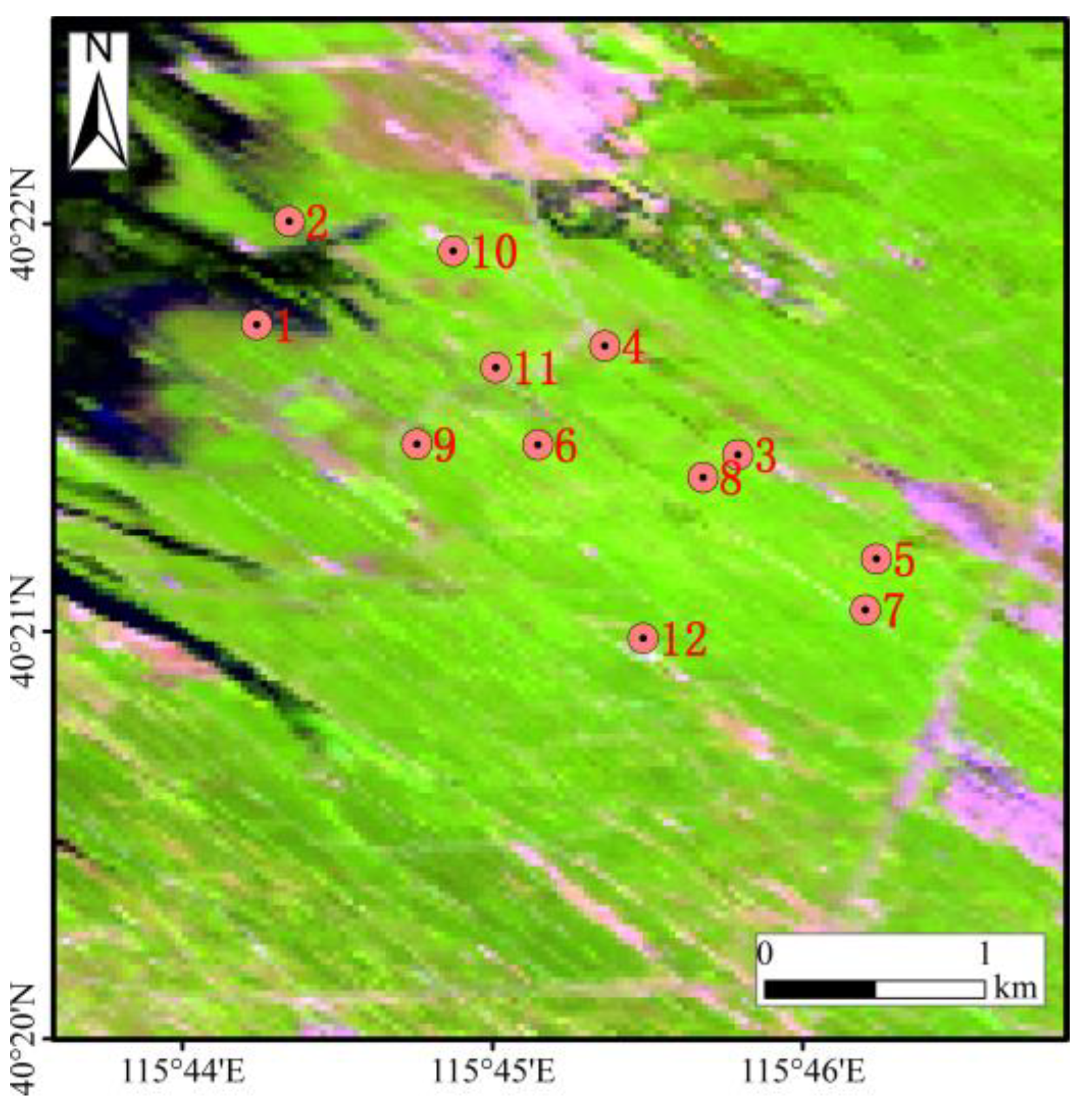
2.1. Study Area

The research was conducted in a 5 km × 5 km region in Huailai, northern China (Figure 1). The annual average precipitation and temperature are 396 mm and 9.6 °C, respectively. Croplands are the main land cover type, and the growing season typically spans from mid-May to late September [50]. The remaining land cover types include water in the northwest and impervious surfaces scattered over the study area.

2.2. Satellite Data

2.2.1. Landsat 8 OLI

We used Landsat 8 Operational Land Imager (OLI) data acquired through the Earth Resources Observation and Science Center Science Processing Architecture (ESPA) (https://espa.cr.usgs.gov). ESPA provides top of canopy reflectances based on the Second Simulation of the Satellite Signal in the Solar Spectrum Vectorial (6SV) atmospheric correction algorithm [51]. Spectral bands in the blue, green, red, near infrared (NIR), and the two shortwave infrared (SWIR1 and SWIR2) bands were used (

Table 1. Band numbers (BN), central wavelengths (CW), and full width at half maximum (FWHM) of the OLI and MODIS sensors for the selected spectral bands.

Spectral band	OLI			MODIS
	BN	CW (nm)	FWHM (nm)	BN	CW (nm)	FWHM (nm)
Blue	2	482.0	60.1	3	469.0	11.5
Green	3	561.4	60.1	4	555.0	12.9
Red	4	654.6	37.5	1	645.0	10.5
Near infrared	5	864.7	28.2	2	858.5	11.6
Short wavelength infrared	6	1608.9	20.4	6	1640.0	14.0
Short wavelength infrared	7	2200.7	84.7	7	2130.0	15.8

).

The dataset includes six cloud-free Landsat 8 OLI scenes (path: 123; row: 32) acquired on the day of year (DOY) 139, 187, 235, 267, 299, and 315 for the year 2013 (Figure 2). This period corresponds to the growing season of the study area (Figure 4). Note that only two Landsat 8 OLI scenes (acquired on DOY 187 and 235) are within the period of acquisition of ground data (from July 1 to September 14, 2013, as detailed in Section 2.3.1), that is, only two ground-based LAI maps could be generated from Landsat data without data blending.

2.2.2. MCD43A4

We also used the nadir directionally normalized reflectance MODIS Nadir Bidirectional Reflectance Distribution Function (BRDF) Adjusted Reflectance product (MCD43A4) [52]. It is produced at 500 m spatial resolution every 8 days using a compositing window of 16 days with data from both Aqua and Terra satellites. All the scenes in 2013 covering the study area (tile number of h24v04) were downloaded from the Land Processes Distributed Active Archive Center (LP DAAC) (https://lpdaac.usgs.gov). The cloud-contaminated scenes were all filtered out, resulting in 36 clean scenes with a full coverage of the growing season of the study area (see Figure 2). The six bands in the MCD43A4 product analogous to the Landsat 8 OLI were selected (Table 1). The MCD43A4 data were resampled to 30-m spatial resolution using the nearest neighbor sampling method.

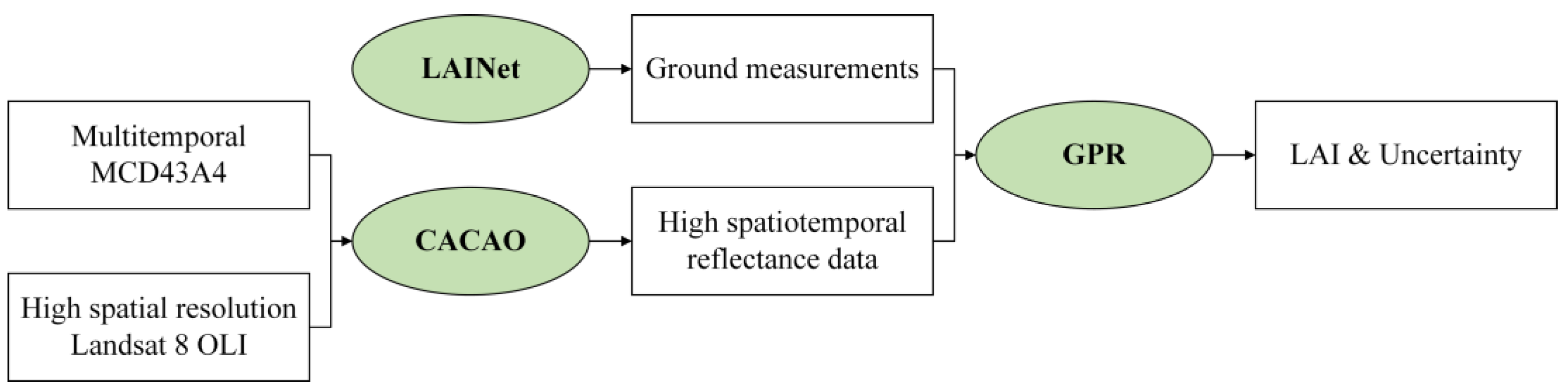
2.3. Retrieval Algorithm

Figure 3 shows the general outline of the proposed framework to generate concomitant LAI and uncertainty maps with high spatiotemporal resolution. It includes LAINet, CACAO, and GPR methods:

(i)

LAINet provided the LAI field measurements for calibrating and validating GPR;

(ii)

CACAO was used for blending the Landsat 8 OLI and MODIS MCD43A4 products and generating reflectance data with high spatiotemporal resolution; and,

(iii)

GPR was used for the retrieval of LAI and uncertainty maps.

2.3.1. LAINet Field Measurements

Field measurements were collected through the LAINet observation system. LAINet comprises 12 below nodes which receive the transmitted solar radiation below the canopy (E_B) (see Figure 1 for their spatial distribution), and 1 above node which receives downward radiation above the canopy (E_A) [42]. The LAI estimation is based on gap fraction measurements calculated as E_B/E_A. For details regarding LAINet, please refer to Qu et al. (2014) and our previous work [8].

Ground measurements were collected from July 1 to September 14, 2013 (see Figure 2). To reduce the random errors, the estimated LAI values from each node of the LAINet observation system were averaged over an 8-day interval. The 8-day composite measurements are hereafter indicated by the DOY of the first day of the compositing period. Due to unexpected instrument failures and unsatisfactory weather conditions, some LAINet measurements were invalid. Only four nodes (numbered 3, 5, 8, and 12 in Figure 1) had valid LAI values for every date. A total of 67 measurements were finally available.

2.3.2. CACAO Reconstruction of High Spatiotemporal Satellite Data

The CACAO [43] method was used to blend Landsat 8 OLI data of high spatial resolution and MCD43A4 data of high temporal resolution, and to reconstruct high spatiotemporal resolution reflectance data.

CACAO is a temporal smoothing and gap filling method with temporal constraints [43]. It fits a phenology model to the actual observations based on a two-step process:

(i)

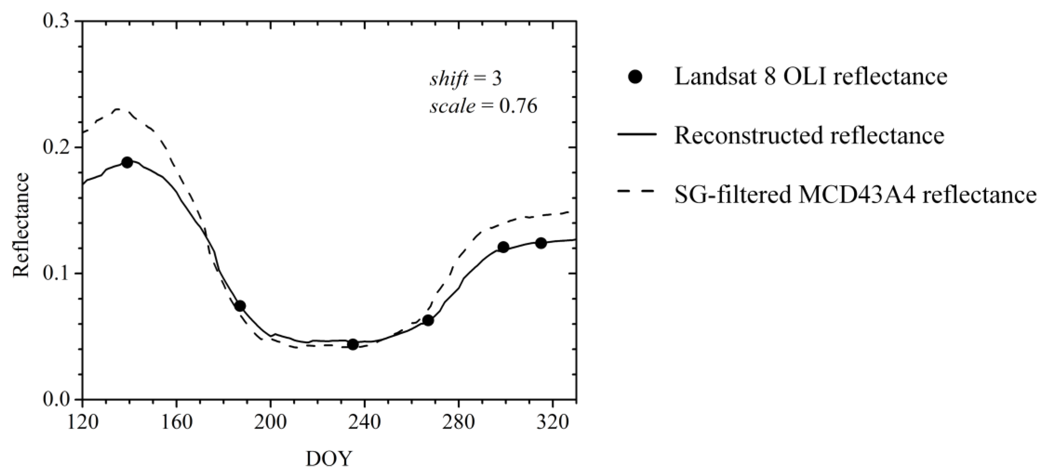
A phenology model was first constructed per pixel and per band based on the temporal evolution of MCD43A4 reflectance data. The time series of MCD43A4 reflectance were smoothed using Savitzky–Golay (SG) filtering [53] to generate the phenology model. SG smooths the time series by fitting a low-degree polynomial in the local temporal window. In this study, the degree of the smoothing polynomial was fixed at 2 and the half-width of the smoothing window at 16 days.

(ii)

The phenology model was then fitted to the actual Landsat observations. It was shifted and scaled in order to minimize its difference with the Landsat 8 OLI data in terms of the root mean square error (RMSE):

$$\arg \underset{scale,shift}{\min }\sqrt{\frac{1}{n}{\displaystyle \sum _{i=1}^n{(R_{OLI}(t_i)-scale·R_{pm}(t_i+shift))}^2}},$$

(1)

where R_OLI represents the Landsat 8 OLI reflectance, R_pm represents the reflectance of the phenology model, n is the number of available Landsat 8 OLI observations (in this study, n = 6), t is the time in days, and scale and shift are the parameters to be adjusted. The minimization of the RMSE was done pixel by pixel, and band by band. After obtaining the values of scale and shift for each pixel in each band, Landsat-like reflectance can be computed at any arbitrary date from the MODIS phenology model.

The CACAO fitting is illustrated in Figure 4. Generally, the Landsat 8 OLI reflectance and the MODIS phenology model (SG-filtered MCD43A4 reflectance) show a similar seasonality with some differences in terms of magnitude and phase. The reconstructed reflectance retains the seasonality of the phenology model and fits the Landsat 8 OLI reflectance values.

The reconstructed reflectances have an 8-day temporal frequency and a 30-m spatial resolution. Their temporal and spatial characteristics inherit from MCD43A4 and Landsat 8 OLI data, respectively. The time series spans from DOY 121 to 321, 2013, covering the entire growing season in our study area.

2.3.3. GPR LAI and Uncertainty Retrieval

GPR can learn the complex relationship between input and output variables based on a probabilistic approach [49]. In addition to highly accurate retrievals, GPR provides pixel-wise confidence intervals of the estimations [7]. Details regarding GPR can be found in a series of studies from Verrelst et al. [7,46,54,55], and we provide only a brief description of GPR adopting their notation.

Under the GPR paradigm, the estimated LAI from GPR obey Gaussian distribution with mean and variance given by the following:

$${\mu }_{*}=K_{*}^{\mathrm{T}}{\left(K+{\sigma }_n^{2}I\right)}^{-1}y,$$

(2)

$${\sigma }_{*}^2=K_{**}-K_{*}^{\mathrm{T}}{\left(K+{\sigma }_n^{2}I\right)}^{-1}{K}_{*},$$

(3)

where K_* is a vector used for characterizing the similarity between the test and training samples, and K_** is the prior covariance. A positive term is subtracted from the prior covariance to estimate the final variance. Therefore, the posterior variance is always smaller than the prior variance, since the observations contribute some additional information [49]. Theoretically, the GPR-estimated uncertainty depends on the training reflectance. If the test reflectance is similar to the training reflectance, the uncertainty for the test set is relatively small because we are dealing with similar input features [46]. In this study, standard deviation (SD), namely, the square root of the predictive variance, was used as a proxy of the retrieval uncertainty.

In Equations (2) and (3), K is a kernel function that evaluates the similarity between the test reflectance x and all training reflectance values. In this study, the automatic relevance determination kernel was used:

$$K(x_i,x_j)=v\exp (-{\displaystyle {\sum }_{b=1}^B\frac{{(x_i^b-x_j^b)}^2}{2{\sigma }_b^2}})+{\delta }_{ij}{\sigma }_n^2,$$

(4)

where v is a scaling factor, B is the dimensions of the input (in this study, B = 6), σ_b controls the spread of the relations for each dimension of the input, and high values of σ_b mean lower informative content of the corresponding dimension for the regression and vice versa, σ_n is the noise standard deviation, and δ_ij is Kronecker’s symbol.

Model hyper-parameters involved in GPR were automatically optimized by maximizing the marginal likelihood in the training set [49]. In this study, GPR was implemented using the simpleR MATLAB toolbox, freely available at https://github.com/IPL-UV/simpleR (accessed on 18 January 2019).

The training dataset is the prerequisite to train a GPR suitable for LAI and uncertainty retrieval. The 67 LAINet measurements and the associated reconstructed Landsat-like reflectances were therefore collected and added to the training dataset. Our study area, beyond the cropping period, is characterized by seasonal inundation and bare soil after harvest. Two dry-soil and two flooded-soil spectral reflectances were therefore added to the training database (with LAI values equal to zero) to improve its representativeness. This treatment was recommended to improve the accuracy of GPR, especially for the input reflectances without associated in situ measurements [34,46]. This resulted in the final training dataset made of 71 LAI-reflectance pairs. The trained GPR was used to generate the concomitant LAI and uncertainty maps with 30-m and 8-day resolutions.

2.4. Validation Approach

The proposed framework approach requires accurate reconstruction of reflectance data at high spatial resolution. The accuracy of the reconstructed reflectances was first assessed (Section 3.1). The original reflectances from the six available Landsat 8 OLI images (Figure 2) were used as the reference data.

We conducted a leave-one-out cross-validation to evaluate the performance of GPR in LAI retrieval (Section 3.2). The n = 67 number of pairs of LAINet-reflectances were split in n-1 for the training and 1 for the validation. Then, the calibrated GPR was used to predict LAI for the observation left out. This process was repeated for all the samples. Finally, we evaluated the performance comparing the predicted LAI with the ground observations for all the samples. For comparison purposes, we also assessed the performance of the exponential regression (ER) approach proposed in our previous work [8]. Both approaches share the same three-step flowchart described in Figure 3, but with some major updates: (1) the exponential regression (y = 0.21exp(3.44x)) proposed in [8] has now been replaced with GPR, to generate LAI and uncertainty maps from ground measurements and high spatiotemporal reflectance data; (2) spectral reflectance was directly ingested into GPR, instead of Normalized Difference Vegetation Index (NDVI) ingested into ER in the previous work; (3) SG filtering was used to generate the phenology model in CACAO, rather than the Double Logistic function adopted in the previous work.

Finally, the temporal evolution of the predicted LAI and associated uncertainties was evaluated (Section 3.3).

3. Results

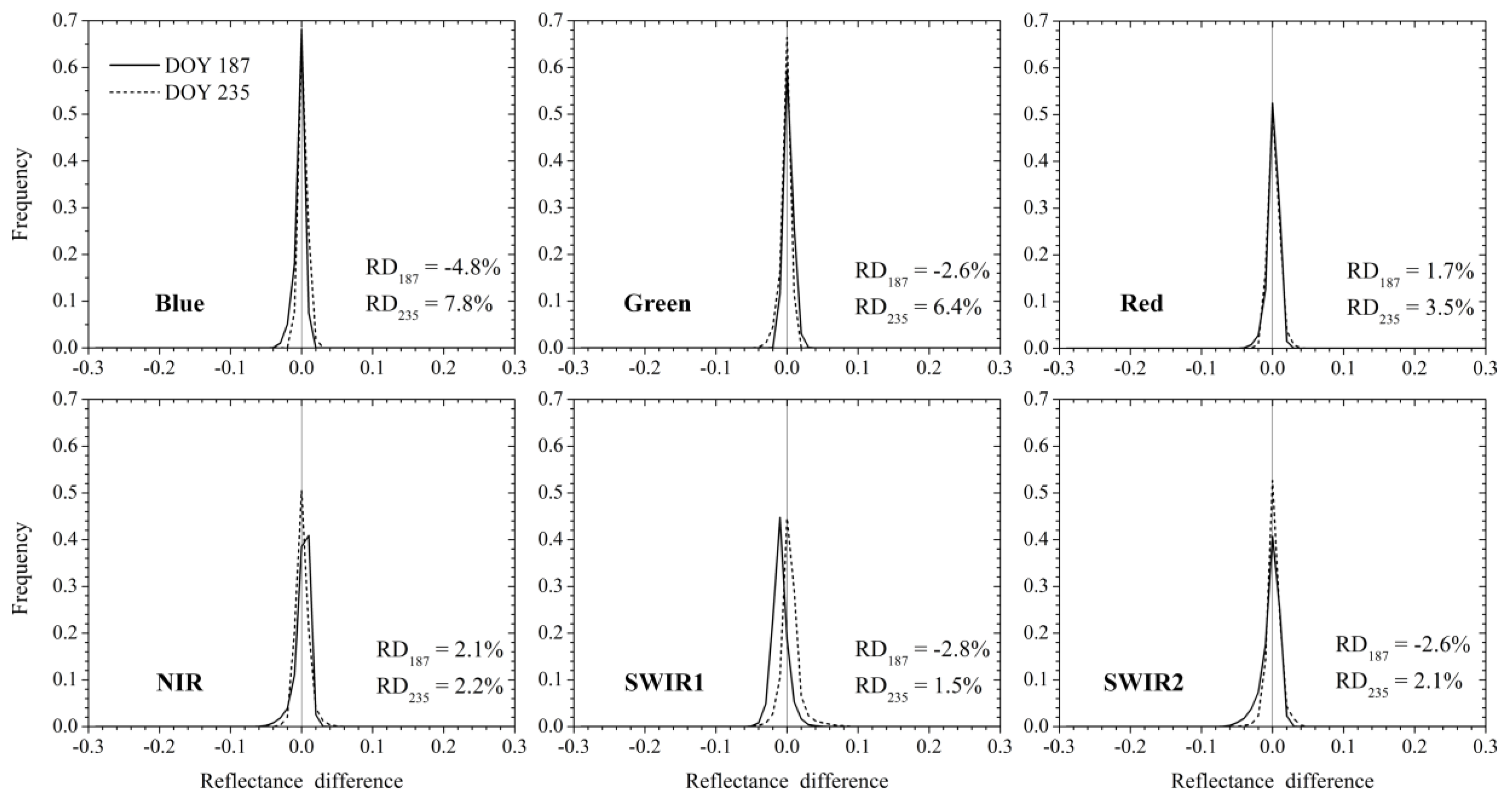
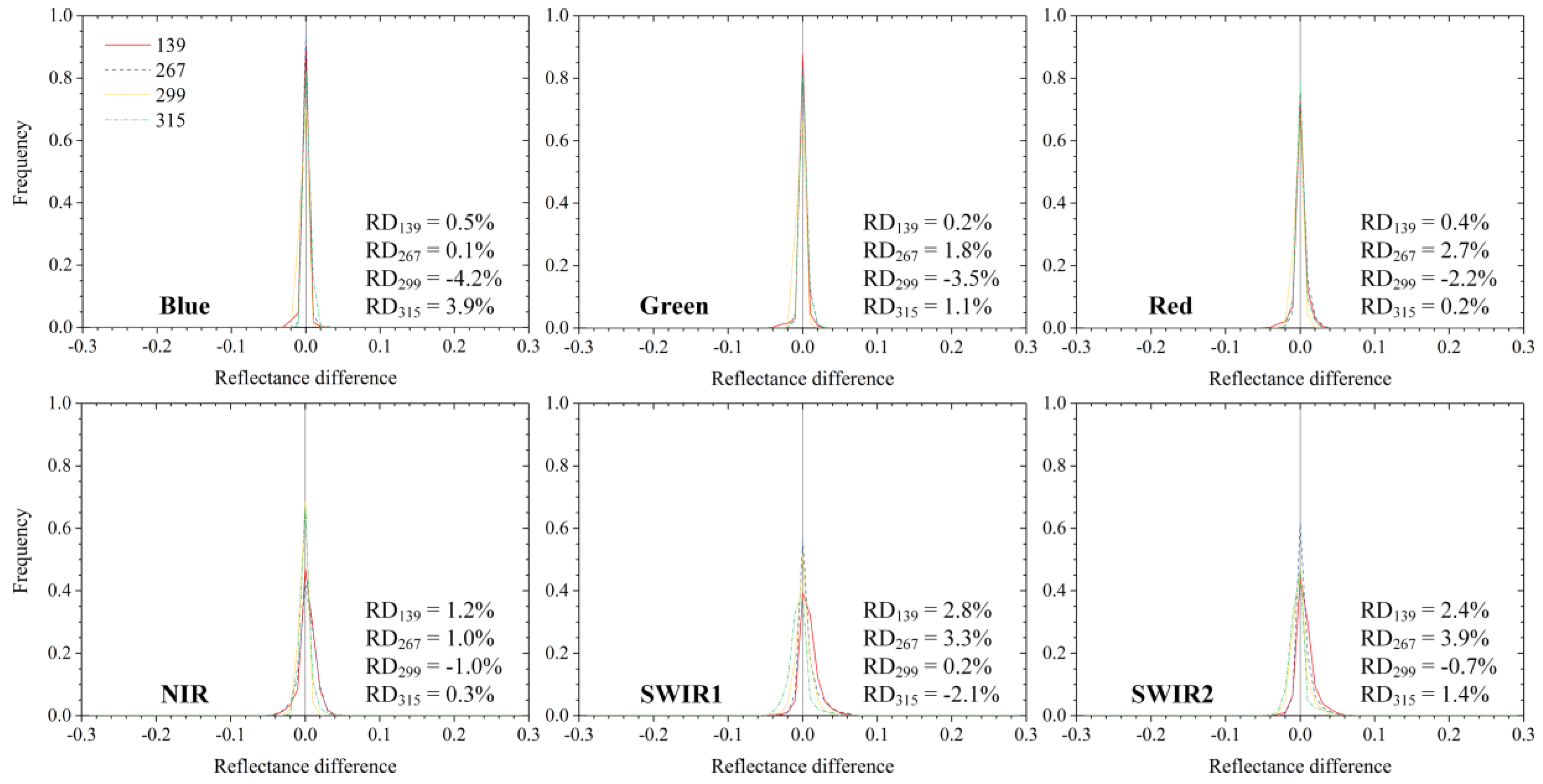
3.1. Evaluation of the Reconstructed High Spatiotemporal Satellite Data

For brevity, Figure 5 only shows the histograms of residuals between the CACAO reconstructed reflectances and OLI observed reflectances on DOY 187 and 235, which are temporally synchronous with the LAINet measurements. The comparison for other dates is shown in Appendix A. In general, the distributions of residuals have peak shapes centered at 0 without significant bias, confirming a good agreement between the reconstructed and the observed reflectances.

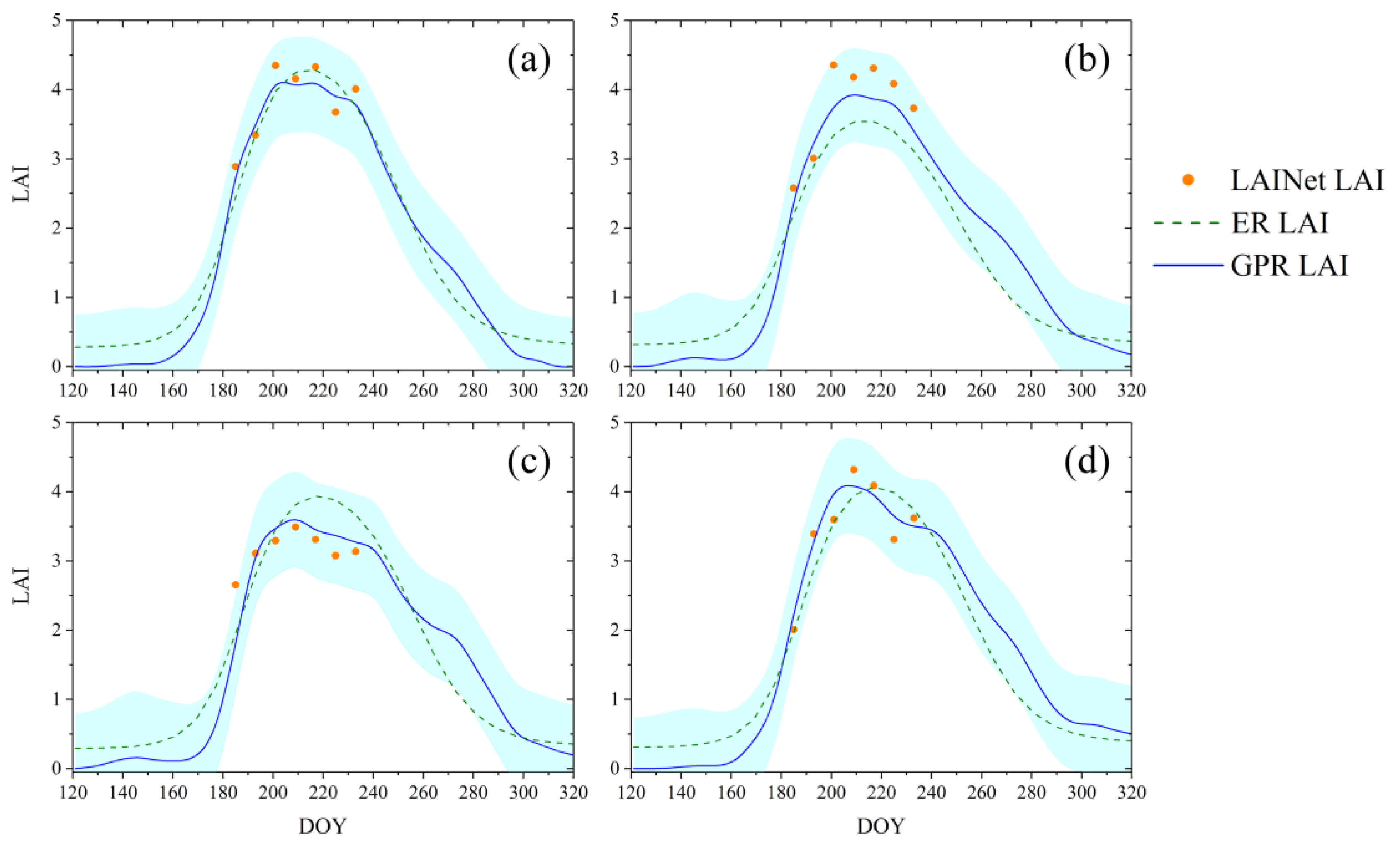
3.2. Cross-Validation

The results of the cross-validation for ER and GPR approaches are shown in Figure 6. Compared to our previous ER approach [8] (R² = 0.70, RMSE = 0.52, relative RMSE (R-RMSE) = 18.4%), GPR showed improved performances (R² = 0.88, RMSE = 0.36, relative RMSE = 12.7%). In addition, ER clearly underestimated LAI observations for LAI values higher than 4.0 because of the saturation of NDVI. This underestimation phenomenon for the high LAI values was clearly mitigated in GPR.

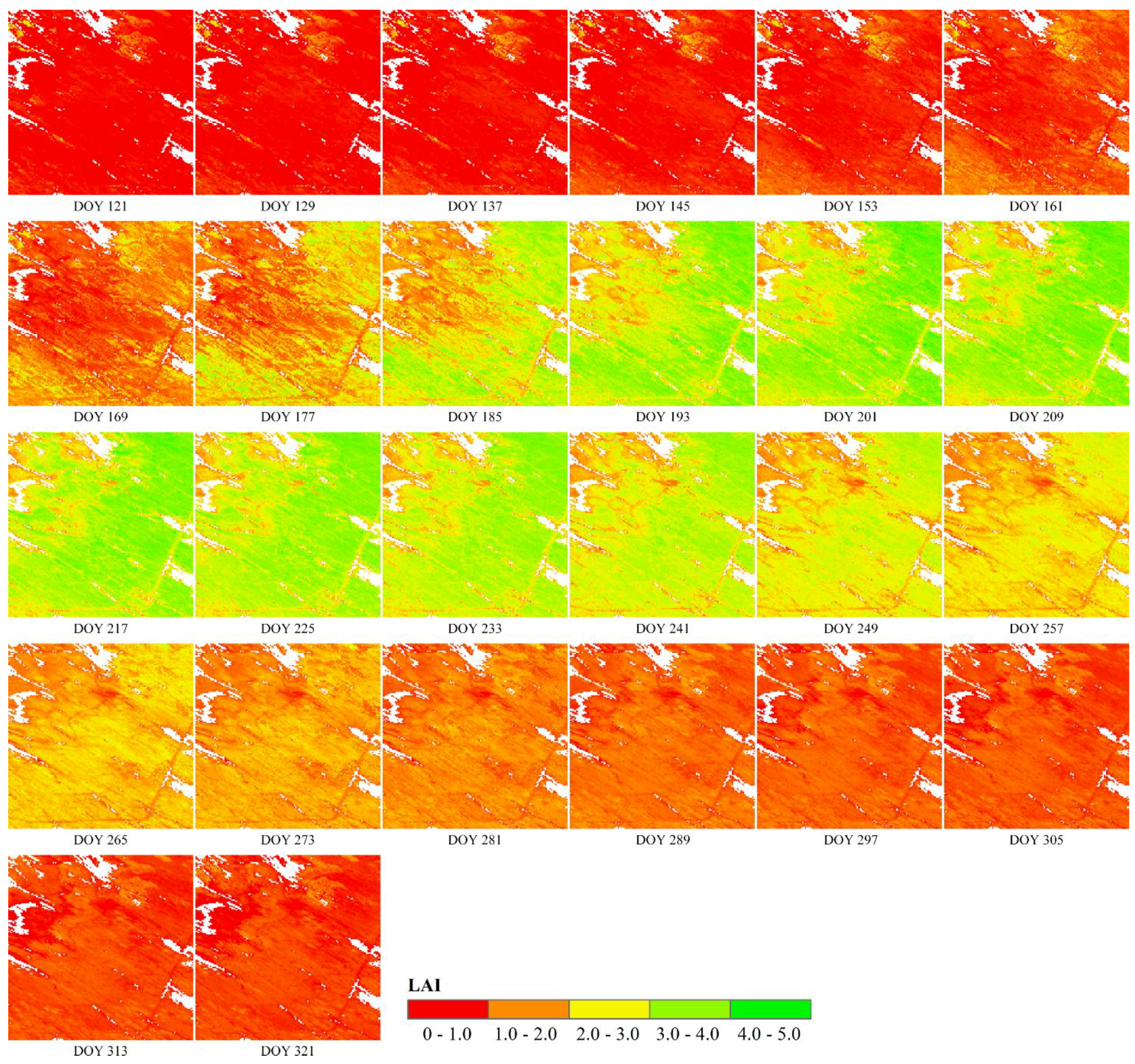
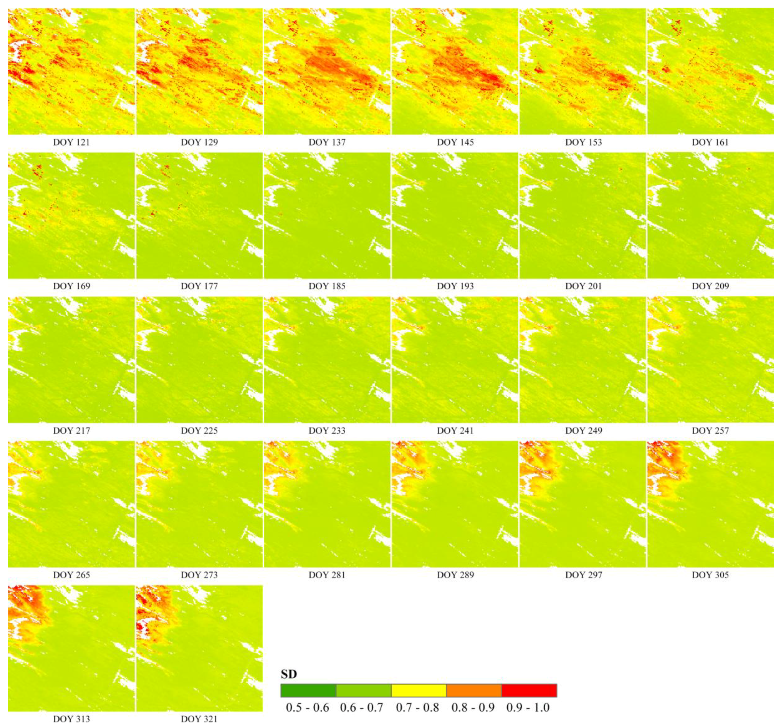
3.3. Temporal Evolution of LAI and Uncertainty Retrievals

The LAI maps (Figure 7) provide detailed information of the expected spatiotemporal dynamics of vegetation in the study area. Before green-up (DOY 161), consistent low LAI values close to zero are observed. After green-up, the vegetation grew rapidly, and reached the growing peak on DOY 217. During this period (from DOY 201 to 217), areas around the water (in the northwestern part of the study area) were characterized by low LAI values (<2.0) due to later sowing. After the growing peak on DOY 217, the vegetation began to wither, and the LAI decreased gradually to zero. During this withering period, areas around the water were also characterized by rather low LAI values, because of seasonal inundation.

The retrieved uncertainty maps (Figure 8) provide insight into the confidence of the estimated LAI. Before green-up, the middle area covering the LAINet nodes was characterized by high uncertainty (SD > 0.8). LAI maps near and during the period of implementation of the LAINet (from DOY 185 to 233) were more credible (SD < 0.7). During the dormancy period (e.g., DOY 289-321), LAI retrievals in the inundated region were uncertain (SD > 0.9).

The temporal evolution of GPR and ER retrievals was further evaluated over the nodes 3, 5, 8 and 12 of LAINet, which provided full temporal coverage for field measurements (Figure 9). In general, both the GPR and ER estimates had similar temporal patterns and followed the temporal dynamics of the observed LAI. However, three main differences can be clearly observed: (1) the local temporal variations in ground LAI measurements were well captured by GPR, whereas the ER over-smoothed the LAI time series; (2) the magnitude of LAI values before green-up (DOY < 161) was close to zero for GPR as expected, whereas ER slightly over-estimated the LAI; (3) during the withering period between DOY 257 and 297, the GPR-estimated LAIs were larger than the ER-estimated ones. Note that nearly all field observations (except the one for plot 8 on DOY 185) lie within the confidence interval of GPR predictions.

4. Discussion

4.1. Improvements Over Previous Approach

This study is based on our previous approach [8] with three major updates: (1) the exponential regression was replaced with GPR, to generate LAI and uncertainty maps from ground measurements and high spatiotemporal reflectance data; (2) spectral reflectance was directly ingested into the transfer function, instead of the vegetation index in the previous work; (3) SG filtering was used to generate the phenology model in CACAO, rather than the Double Logistic function adopted previously. These updates bring several improvements. First, the accuracy of the retrievals has improved. The R² increased from 0.70 to 0.88, and the RMSE decreased from 0.52 LAI (18.4%) to 0.36 LAI (12.7%), meeting the accuracy requirements proposed by the Global Climate Observing System [44]. Second, the temporal evolution of LAI is better captured by GPR, whereas ER over-smooths the time series. Further, GPR shows a better temporal extrapolation capacity than ER, particularly for the dormancy period with LAI retrievals close to the expected zero LAI value. This allows the generation of temporally continuous LAI maps over the entire growing season. Finally, GPR provides the uncertainty associated with the LAI retrievals [46,54].

Several reasons can explain this improvement. (1) GPR is an advanced regression method and can learn the complex nonlinear relationship between remote sensing observations and biophysical variables [48,49]. Many studies have shown that GPR outperforms parametric regression methods in most cases [5,7,34]. Our study further confirms this finding. (2) GPR has the capability to directly exploit the full spectrum [55] and, for this reason, individual bands rather than the derived vegetation index were used in our GPR. The procedure for calculating the vegetation index (i.e., the selection of bands and the formulation of the selected bands) would cause loss of information useful for LAI retrieval [56]. (3) SG filtering can reserve the relatively high frequency variation in the original reflectance time series [53], which is therefore suitable for capturing the local scale changes in the time series of LAI and preventing the over-smoothing observed in Double Logistic. (4) Two dry-soil and two flooded-soil spectral reflectances (with LAI values equal to zero) were introduced to establish an extended training dataset. The original training dataset consisting of only the 67 LAINet measurements under-sampled the low LAI values. The introduction of dry- and flooded-soil spectral reflectances improved the representativeness of the trained GPR for low LAI values, and therefore improved its temporal extrapolation capacity especially for dormancy periods.

The GPR-estimated LAI values are higher than the ER retrievals during the withering period (see Figure 9). One possible explanation is that the NDVI represents the greenness of the vegetation [57], and the gradual decrease of leaf chlorophyll content during the withering period [58] can therefore decrease the value of NDVI and further cause an underestimation of the LAI value. The temporal variation of leaf chlorophyll content (which further causes the variation of leaf spectra) underlines the importance of the direct use of multi- or even hyper-spectral reflectances, especially those containing information on leaf spectra.

4.2. Potential Applications

The LAI time series generated from the proposed framework are characterized by high spatiotemporal resolution and are accompanied with concomitant uncertainty maps. These datasets may be useful in many applications.

The generated high spatiotemporal resolution LAI maps can support the validation activities for the coarse resolution LAI products. Our framework complies with the hierarchical four-stage validation approach proposed by the Land Product Validation (LPV) subgroup of the Committee Earth Observing Satellites’ Working Group on Calibration and Validation (CEOS WGCV) [59]. Therefore, the generated LAI maps can directly serve as reference maps in validation activities. The obvious advantage of our framework over existing studies is that it can derive temporally continuous LAI reference maps. Therefore, it can be used to assess the temporal performance of the coarse resolution LAI products, which is the prerequisite for long-term global change research [60,61].

The derived high spatiotemporal resolution LAI maps can also be used to quantify the spatial and temporal variability of crop distribution and status at field scale. This kind of information is of paramount importance for precision agriculture [62]. The high spatiotemporal resolution LAI maps can provide guidance on agricultural activities and aid farmers to decide, for example, which is the appropriate time to fertilize or irrigate their fields.

The retrieved uncertainty information would allow a proper use of the LAI retrieval. For example, the high reliable retrieval with low SD can be easily extracted for subsequent applications. The inconsistencies among existing coarse resolution LAI products call for quality-assured long-term LAI products [60,63]. Our framework may provide an effective method to fulfill this target.

In addition, the concomitant uncertainty maps facilitate the integration of remote sensing and process models at field scale [64]. For example, the LAI retrievals can be easily assimilated by crop models, because their contribution in the assimilation process can be automatically weighted according to the concomitant uncertainty maps.

4.3. Future Prospects of Research

This study proposed a framework to generate concomitant LAI and uncertainty maps with high spatiotemporal resolution. Several issues are worth being noted to further improve the framework.

High spatial resolution remote sensing observations that are temporally synchronous with field measurements are needed to reduce the uncertainty during LAI estimation caused by the dynamic change of vegetation [65]. The tradeoff between temporal and spatial resolutions of a remote sensing sensor makes it difficult to acquire remote sensing observation with both high spatial resolution and frequent coverage. Data blending techniques were used here to obtain high spatial resolution remote sensing observations that were temporally synchronous with LAINet observations. In our study area, one year of MODIS data was enough to provide temporally continuous coverage although multi-year data may be required to build the phenology model in regions with high cloud coverage. Note that a spectral normalization between MCD43A4 and Landsat 8 OLI data was not applied. We assumed that the difference in their spectral response functions could be implicitly accounted for during the shifting and scaling procedure, considering the significant linear correlation between MODIS and OLI reflectance products [51].

An alternative to generate high spatiotemporal resolution remote sensing data is the combined use of multi-sensor data. For example, Zhao et al. [16] used HJ1/CCD and Landsat 8/OLI simultaneously to fill temporal gaps which existed in any one single data source. In addition, some newly launched satellites (e.g., GF-6 or Venµs) can provide remote sensing observations with both high spatial and temporal resolutions. The performance of our proposed method for multi-sensor or high spatiotemporal data will be evaluated in future studies.

The analysis of the uncertainty maps suggested that under-sampled observations (e.g., middle areas before green-up and inundated areas during the dormancy period, see Figure 9) are often associated with high uncertainty. Therefore, a longer temporal span and more below nodes should be added to the LAINet system in our study area to enhance the representativeness of the training dataset [50,66]. To partly cope with the training dataset under-sample for low LAI, we deliberately extended the original training dataset with four new spectra that covered two main kinds of non-vegetated surfaces (i.e., dry and flooded soils) with an LAI value of zero. This extended training dataset improved the extrapolation capacity of GPR, especially for low values which were not sufficiently sampled by LAINet. Surprisingly, the estimates with low LAI also represent high uncertainty after introducing the non-vegetated spectra. This may be because the non-vegetated and low-LAI surfaces have significant heterogeneity [67] and four spectra cannot represent them very well. However, we did not try to add more non-vegetated spectra, because the number of LAINet measurements was limited (67), and more non-vegetated spectra would have diluted the information involved in LAINet measurements, and further reduced the retrieval accuracy. Another solution to improve the representativeness of the training dataset is to add reflectance simulated by RT models, which can cover a broader range of scenarios. As proposed by [12], the simulated reflectance can be imported through the joint Gaussian process to extrapolate the observed reflectance.

The predictive variance from GPR is an indicator of the real uncertainty; however, the physical meaning of this predictive variance is still not clear [46]. Intuitively, it is an indicator of the similarity between the test and the training samples in the LAI space transferred from the reflectance space through a kernel function (see Equation (4)). The kernel used assumed that the measurement noise was independent from the signal (see Equation (4)), which does not hold in most of the problems. The heteroscedastic Gaussian processes [68] can be employed to further improve the estimation results in future studies. In addition, several other methods exist in the literature to quantify the uncertainty associated with retrievals including partial least squares regression [69], Markov chain Monte Carlo [70], random forest [71], and Kriging [72]. These methods will be assessed in future studies.

5. Conclusions

We proposed a framework to generate long-term time series of LAI and their associated uncertainty maps with high spatiotemporal resolution. It was based on the combination of LAINet, CACAO, and GPR. The performance of the proposed method was evaluated over the entire growing season in a crop site in northern China. The accuracy of the retrieved LAI maps (0.36 LAI (12.7%) in terms of RMSE with R² = 0.88 correlation) met the up-to-date uncertainty threshold (15%) proposed by the Global Climate Observing System. To our knowledge, this is the first work combining wireless sensor network, data blending, and machine learning technologies for retrieving LAI and its uncertainty at high spatiotemporal resolution. Our framework will contribute to precision agriculture, as well as to the retrieval and validation of LAI products.

References

1. Wang, G.L.; Yu, M.; Pal, J.S.; Mei, R.; Bonan, G.B.; Levis, S.; Thornton, P.E. On the development of a coupled regional climate-vegetation model RCM-CLM-CN-DV and its validation in Tropical Africa. Clim. Dyn. 2016, 46, 515–539. [Google Scholar] [CrossRef]
2. Liu, J.; Chen, J.M.; Cihlar, J.; Park, W.M. A process-based boreal ecosystem productivity simulator using remote sensing inputs. Remote Sens. Environ. 1997, 62, 158–175. [Google Scholar] [CrossRef]
3. Serbin, S.P.; Ahl, D.E.; Gower, S.T. Spatial and temporal validation of the MODIS LAI and FPAR products across a boreal forest wildfire chronosequence. Remote Sens. Environ. 2013, 133, 71–84. [Google Scholar] [CrossRef]
4. Myneni, R.B.; Hoffman, S.; Knyazikhin, Y.; Privette, J.L.; Glassy, J.; Tian, Y.; Wang, Y.; Song, X.; Zhang, Y.; Smith, G.R.; et al. Global products of vegetation leaf area and fraction absorbed PAR from year one of MODIS data. Remote Sens. Environ. 2002, 83, 214–231. [Google Scholar] [CrossRef] [Green Version]
5. García-Haro, F.J.; Campos-Taberner, M.; Muñoz-Marí, J.; Laparra, V.; Camacho, F.; Sánchez-Zapero, J.; Camps-Valls, G. Derivation of global vegetation biophysical parameters from EUMETSAT Polar System. ISPRS J. Photogramm. Remote Sens. 2018, 139, 57–74. [Google Scholar] [CrossRef]
6. Heiskanen, J.; Rautiainen, M.; Stenberg, P.; Mottus, M.; Vesanto, V.H. Sensitivity of narrowband vegetation indices to boreal forest LAI, reflectance seasonality and species composition. ISPRS J. Photogramm. 2013, 78, 1–14. [Google Scholar] [CrossRef]
7. Verrelst, J.; Munoz, J.; Alonso, L.; Delegido, J.; Rivera, J.P.; Camps-Valls, G.; Moreno, J. Machine learning regression algorithms for biophysical parameter retrieval: Opportunities for Sentinel-2 and -3. Remote Sens. Environ. 2012, 118, 127–139. [Google Scholar] [CrossRef]
8. Yin, G.F.; Li, A.N.; Jin, H.A.; Zhao, W.; Bian, J.H.; Qu, Y.H.; Zeng, Y.L.; Xu, B.D. Derivation of temporally continuous LAI reference maps through combining the LAINet observation system with CACAO. Agric. For. Meteorol. 2017, 233, 209–221. [Google Scholar] [CrossRef]
9. Houborg, R.; McCabe, M.; Cescatti, A.; Gao, F.; Schull, M.; Gitelson, A. Joint leaf chlorophyll content and leaf area index retrieval from Landsat data using a regularized model inversion system (REGFLEC). Remote Sens. Environ. 2015, 159, 203–221. [Google Scholar] [CrossRef] [Green Version]
10. Laurent, V.C.E.; Schaepman, M.E.; Verhoef, W.; Weyermann, J.; Chavez, R.O. Bayesian object-based estimation of LAI and chlorophyll from a simulated Sentinel-2 top-of-atmosphere radiance image. Remote Sens. Environ. 2014, 140, 318–329. [Google Scholar] [CrossRef]
11. Zeng, Y.; Li, J.; Liu, Q.; Huete, A.R.; Yin, G.; Xu, B.; Fan, W.; Zhao, J.; Yan, K.; Mu, X. A Radiative Transfer Model for Heterogeneous Agro-Forestry Scenarios. IEEE Trans. Geosci. Remote Sens. 2016, 54, 4613–4628. [Google Scholar] [CrossRef]
12. Svendsen, D.H.; Martino, L.; Campos-Taberner, M.; Garcia-Haro, F.J.; Camps-Valls, G. Joint Gaussian Processes for Biophysical Parameter Retrieval. IEEE Trans. Geosci. Remote Sens. 2017, 1–10. [Google Scholar] [CrossRef]
13. Teubner, I.E.; Forkel, M.; Jung, M.; Liu, Y.Y.; Miralles, D.G.; Parinussa, R.; van der Schalie, R.; Vreugdenhil, M.; Schwalm, C.R.; Tramontana, G.; et al. Assessing the relationship between microwave vegetation optical depth and gross primary production. Int. J. Appl. Earth Obs. Geoinf. 2018, 65, 79–91. [Google Scholar] [CrossRef]
14. Verrelst, J.; Camps-Valls, G.; Munoz-Mari, J.; Rivera, J.P.; Veroustraete, F.; Clevers, J.; Moreno, J. Optical remote sensing and the retrieval of terrestrial vegetation bio-geophysical properties—A review. ISPRS J. Photogramm. 2015, 108, 273–290. [Google Scholar] [CrossRef]
15. Zeng, Y.; Xu, B.; Yin, G.; Wu, S.; Hu, G.; Yan, K.; Yang, B.; Song, W.; Li, J. Spectral Invariant Provides a Practical Modeling Approach for Future Biophysical Variable Estimations. Remote Sens. 2018, 10, 1508. [Google Scholar] [CrossRef]
16. Zhao, J.; Li, J.; Liu, Q.; Fan, W.; Zhong, B.; Wu, S.; Yang, L.; Zeng, Y.; Xu, B.; Yin, G. Leaf Area Index Retrieval Combining HJ1/CCD and Landsat8/OLI Data in the Heihe River Basin, China. Remote Sens. 2015, 7, 6862–6885. [Google Scholar] [CrossRef] [Green Version]
17. Yin, G.F.; Li, J.; Liu, Q.H.; Fan, W.L.; Xu, B.D.; Zeng, Y.L.; Zhao, J. Regional leaf area index retrieval based on remote sensing: The role of radiative transfer model selection. Remote Sens. 2015, 7, 4604–4625. [Google Scholar] [CrossRef]
18. Quan, X.W.; He, B.B.; Li, X. A Bayesian network-based method to alleviate the ill-posed inverse problem: A case study on leaf area index and canopy water content retrieval. IEEE Trans. Geosci. Remote Sens. 2015, 53, 6507–6517. [Google Scholar] [CrossRef]
19. Zeng, Y.; Li, J.; Liu, Q.; Huete, A.R.; Xu, B.; Yin, G.; Zhao, J.; Yang, L.; Fan, W.; Wu, S.; et al. An Iterative BRDF/NDVI Inversion Algorithm Based on A Posteriori Variance Estimation of Observation Errors. IEEE Trans. Geosci. Remote Sens. 2016, 54, 6481–6496. [Google Scholar] [CrossRef]
20. Breda, N.J.J. Ground-based measurements of leaf area index: A review of methods, instruments and current controversies. J. Exp. Bot. 2003, 54, 2403–2417. [Google Scholar] [CrossRef]
21. Jonckheere, I.; Fleck, S.; Nackaerts, K.; Muys, B.; Coppin, P.; Weiss, M.; Baret, F. Review of methods for in situ leaf area index determination—Part I. Theories, sensors and hemispherical photography. Agric. For. Meteorol. 2004, 121, 19–35. [Google Scholar] [CrossRef]
22. Weiss, M.; Baret, F.; Smith, G.J.; Jonckheere, I.; Coppin, P. Review of methods for in situ leaf area index (LAI) determination Part II. Estimation of LAI, errors and sampling. Agric. For. Meteorol. 2004, 121, 37–53. [Google Scholar] [CrossRef]
23. Zeng, Y.; Li, J.; Liu, Q.; Hu, R.; Mu, X.; Fan, W.; Xu, B.; Yin, G.; Wu, S. Extracting Leaf Area Index by Sunlit Foliage Component from Downward-Looking Digital Photography under Clear-Sky Conditions. Remote Sens. 2015, 7, 13410–13435. [Google Scholar] [CrossRef] [Green Version]
24. Demarez, V.; Duthoit, S.; Baret, F.; Weiss, M.; Dedieu, G. Estimation of leaf area and clumping indexes of crops with hemispherical photographs. Agric. For. Meteorol. 2008, 148, 644–655. [Google Scholar] [CrossRef] [Green Version]
25. Leblanc, S.G. Correction to the plant canopy gap-size analysis theory used by the Tracing Radiation and Architecture of Canopies instrument. Appl. Opt. 2002, 41, 7667–7670. [Google Scholar] [CrossRef] [PubMed]
26. LI-COR. LAI-2000 Plant Canopy Analyzer Operating Manual. 1991. Available online: http://www.ecotek.com.cn/download/Manual-LAI-2000-EN.pdf (accessed on 23 January 2019).
27. Ryu, Y.; Lee, G.; Jeon, S.; Song, Y.; Kimm, H. Monitoring multi-layer canopy spring phenology of temperate deciduous and evergreen forests using low-cost spectral sensors. Remote Sens. Environ. 2014, 149, 227–238. [Google Scholar] [CrossRef]
28. Campos-Taberner, M.; Garcia-Haro, F.J.; Confalonieri, R.; Martinez, B.; Moreno, A.; Sanchez-Ruiz, S.; Gilabert, M.A.; Camacho, F.; Boschetti, M.; Busetto, L. Multitemporal monitoring of plant area index in the Valencia rice district with PocketLAI. Remote Sens. 2016, 8, 202. [Google Scholar] [CrossRef]
29. Qu, Y.H.; Wang, J.; Song, J.L.; Wang, J.D. Potential and limits of retrieving conifer leaf area index using smartphone-based method. Forests 2017, 8, 217. [Google Scholar] [CrossRef]
30. Yan, K.; Park, T.; Yan, G.J.; Chen, C.; Yang, B.; Liu, Z.; Nemani, R.R.; Knyazikhin, Y.; Myneni, R.B. Evaluation of MODIS LAI/FPAR product collection 6. Part 1: Consistency and improvements. Remote Sens. 2016, 8, 359. [Google Scholar] [CrossRef]
31. Liang, S.L.; Zhao, X.; Liu, S.H.; Yuan, W.P.; Cheng, X.; Xiao, Z.Q.; Zhang, X.T.; Liu, Q.; Cheng, J.; Tang, H.R.; et al. A long-term Global LAnd Surface Satellite (GLASS) data-set for environmental studies. Int. J. Digit. Earth 2013, 6, 5–33. [Google Scholar] [CrossRef] [Green Version]
32. Baret, F.; Weiss, M.; Lacaze, R.; Camacho, F.; Makhmara, H.; Pacholcyzk, P.; Smets, B. GEOV1: LAI and FAPAR essential climate variables and FCOVER global time series capitalizing over existing products. Part1: Principles of development and production. Remote Sens. Environ. 2013, 137, 299–309. [Google Scholar] [CrossRef]
33. Verger, A.; Baret, F.; Weiss, M. Near real-time vegetation monitoring at global scale. IEEE J. Sel. Top. Appl. Earth Obs. Remote. Sens. 2014, 7, 3473–3481. [Google Scholar] [CrossRef]
34. Campos-Taberner, M.; García-Haro, F.J.; Camps-Valls, G.; Grau-Muedra, G.; Nutini, F.; Crema, A.; Boschetti, M. Multitemporal and multiresolution leaf area index retrieval for operational local rice crop monitoring. Remote Sens. Environ. 2016, 187, 102–118. [Google Scholar] [CrossRef]
35. Ganguly, S.; Nemani, R.R.; Zhang, G.; Hashimoto, H.; Milesi, C.; Michaelis, A.; Wang, W.; Votava, P.; Samanta, A.; Melton, F. Generating global leaf area index from Landsat: Algorithm formulation and demonstration. Remote Sens. Environ. 2012, 122, 185–202. [Google Scholar] [CrossRef]
36. Houborg, R.; McCabe, M.F. A hybrid training approach for leaf area index estimation via Cubist and random forests machine-learning. ISPRS J. Photogramm. Remote Sens. 2018, 135, 173–188. [Google Scholar] [CrossRef]
37. Zhu, X.; Helmer, E.H.; Gao, F.; Liu, D.; Chen, J.; Lefsky, M.A. A flexible spatiotemporal method for fusing satellite images with different resolutions. Remote Sens. Environ. 2016, 172, 165–177. [Google Scholar] [CrossRef]
38. Xu, B.; Li, J.; Liu, Q.; Huete, A.R.; Yu, Q.; Zeng, Y.; Yin, G.; Zhao, J.; Yang, L. Evaluating Spatial Representativeness of Station Observations for Remotely Sensed Leaf Area Index Products. IEEE J. Sel. Top. Appl. Earth Obs. Remote. Sens. 2016, 9, 3267–3282. [Google Scholar] [CrossRef]
39. Yin, G.F.; Li, J.; Liu, Q.H.; Li, L.H.; Zeng, Y.L.; Xu, B.D.; Yang, L.; Zhao, J. Improving leaf area index retrieval over heterogeneous surface by integrating textural and contextual information: A case study in the Heihe River Basin. IEEE Geosci. Remote Sens. Lett. 2015, 12, 359–363. [Google Scholar] [CrossRef]
40. Zeng, Y.L.; Li, J.; Liu, Q.H.; Li, L.H.; Xu, B.D.; Yin, G.F.; Peng, J.J. A Sampling Strategy for Remotely Sensed LAI Product Validation Over Heterogeneous Land Surfaces. IEEE J. Sel. Top. Appl. Earth Obs. Remote Sens. 2014, 7, 3128–3142. [Google Scholar] [CrossRef]
41. Dou, B.; Wen, J.; Li, X.; Liu, Q.; Peng, J.; Xiao, Q.; Zhang, Z.; Tang, Y.; Wu, X.; Lin, X.; et al. Wireless Sensor Network of Typical Land Surface Parameters and Its Preliminary Applications for Coarse-Resolution Remote Sensing Pixel. Int. J. Distrib. Sens. Netw. 2016. [Google Scholar] [CrossRef]
42. Qu, Y.H.; Han, W.C.; Fu, L.Z.; Li, C.R.; Song, J.L.; Zhou, H.M.; Bo, Y.C.; Wang, J.D. LAINet—A wireless sensor network for coniferous forest leaf area index measurement: Design, algorithm and validation. Comput. Electron. Agric. 2014, 108, 200–208. [Google Scholar] [CrossRef]
43. Verger, A.; Baret, F.; Weiss, M.; Kandasamy, S.; Vermote, E. The CACAO method for smoothing, gap filling, and characterizing seasonal anomalies in satellite time series. IEEE Trans. Geosci. Remote Sens. 2013, 51, 1963–1972. [Google Scholar] [CrossRef]
44. GCOS. The Global Observing System for Climate: Implementation Needs. 2016. Available online: https://unfccc.int/sites/default/files/gcos_ip_10oct2016.pdf (accessed on 23 January 2019).
45. Fang, H.; Wei, S.; Jiang, C.; Scipal, K. Theoretical uncertainty analysis of global MODIS, CYCLOPES, and GLOBCARBON LAI products using a triple collocation method. Remote Sens. Environ. 2012, 124, 610–621. [Google Scholar] [CrossRef]
46. Verrelst, J.; Rivera, J.P.; Moreno, J.; Camps-Valls, G. Gaussian processes uncertainty estimates in experimental Sentinel-2 LAI and leaf chlorophyll content retrieval. ISPRS J. Photogramm. Remote Sens. 2013, 86, 157–167. [Google Scholar] [CrossRef]
47. Han, W.C.; Qu, Y.H. Data uncertainty in an improved Bayesian network and evaluations of the credibility of the retrieved multitemporal high-spatial-resolution leaf area index. IEEE J. Sel. Top. Appl. Earth Obs. Remote. Sens. 2016, 9, 3553–3563. [Google Scholar] [CrossRef]
48. Camps-Valls, G.; Gómez-Chova, L.; Muñoz-Marí, J.; Vila-Francés, J.; Amorós, J.; Valle-Tascon, S.D.; Calpe-Maravilla, J. Biophysical parameter estimation with adaptive Gaussian processes. In Proceedings of the 2009 IEEE International Geoscience and Remote Sensing Symposium, Cape Town, South Africa, 12–17 July 2009; pp. IV-69–IV-72. [Google Scholar]
49. Rasmussen, C.E.; Williams, C.K. Gaussian Processes for Machine Learning; MIT Press: Cambridge, MA, USA, 2006; Volume 2, p. 4. [Google Scholar]
50. Zeng, Y.L.; Li, J.; Liu, Q.H.; Qu, Y.H.; Huete, A.R.; Xu, B.D.; Yin, G.F.; Zhao, J. An Optimal Sampling Design for Observing and Validating Long-Term Leaf Area Index with Temporal Variations in Spatial Heterogeneities. Remote Sens. 2015, 7, 1300–1319. [Google Scholar] [CrossRef] [Green Version]
51. Vermote, E.; Justice, C.; Claverie, M.; Franch, B. Preliminary analysis of the performance of the Landsat 8/OLI land surface reflectance product. Remote Sens. Environ. 2016, 185, 46–56. [Google Scholar] [CrossRef]
52. Schaaf, C.B.; Gao, F.; Strahler, A.H.; Lucht, W.; Li, X.W.; Tsang, T.; Strugnell, N.C.; Zhang, X.Y.; Jin, Y.F.; Muller, J.P.; et al. First operational BRDF, albedo nadir reflectance products from MODIS. Remote Sens. Environ. 2002, 83, 135–148. [Google Scholar] [CrossRef] [Green Version]
53. Chen, J.; Jonsson, P.; Tamura, M.; Gu, Z.H.; Matsushita, B.; Eklundh, L. A simple method for reconstructing a high-quality NDVI time-series data set based on the Savitzky-Golay filter. Remote Sens. Environ. 2004, 91, 332–344. [Google Scholar] [CrossRef]
54. Verrelst, J.; Alonso, L.; Camps-Valls, G.; Delegido, J.; Moreno, J. Retrieval of vegetation biophysical parameters using Gaussian process techniques. IEEE Trans. Geosci. Remote Sens. 2012, 50, 1832–1843. [Google Scholar] [CrossRef]
55. Verrelst, J.; Rivera, J.P.; Veroustraete, F.; Munoz-Mari, J.; Clevers, J.; Camps-Valls, G.; Moreno, J. Experimental Sentinel-2 LAI estimation using parametric, non-parametric and physical retrieval methods—A comparison. ISPRS J. Photogramm. 2015, 108, 260–272. [Google Scholar] [CrossRef]
56. Xie, Q.; Huang, W.; Zhang, B.; Chen, P.; Song, X.; Pascucci, S.; Pignatti, S.; Laneve, G.; Dong, Y. Estimating winter wheat leaf area index from ground and hyperspectral observations using vegetation indices. IEEE J. Sel. Top. Appl. Earth Obs. Remote. Sens. 2016, 9, 771–780. [Google Scholar] [CrossRef]
57. Huete, A.; Didan, K.; Miura, T.; Rodriguez, E.P.; Gao, X.; Ferreira, L.G. Overview of the radiometric and biophysical performance of the MODIS vegetation indices. Remote Sens. Environ. 2002, 83, 195–213. [Google Scholar] [CrossRef]
58. Croft, H.; Chen, J.M.; Luo, X.Z.; Bartlett, P.; Chen, B.; Staebler, R.M. Leaf chlorophyll content as a proxy for leaf photosynthetic capacity. Glob. Chang. Biol. 2017, 23, 3513–3524. [Google Scholar] [CrossRef] [PubMed]
59. Morisette, J.T.; Baret, F.; Privette, J.L.; Myneni, R.B.; Nickeson, J.E.; Garrigues, S.; Shabanov, N.V.; Weiss, M.; Fernandes, R.A.; Leblanc, S.G.; et al. Validation of global moderate-resolution LAI products: A framework proposed within the CEOS Land Product Validation subgroup. IEEE Trans. Geosci. Remote Sens. 2006, 44, 1804–1817. [Google Scholar] [CrossRef]
60. Jiang, C.Y.; Ryu, Y.; Fang, H.L.; Myneni, R.; Claverie, M.; Zhu, Z.C. Inconsistencies of interannual variability and trends in long-term satellite leaf area index products. Glob. Chang. Biol. 2017, 23, 4133–4146. [Google Scholar] [CrossRef] [PubMed] [Green Version]
61. Smettem, K.R.J.; Waring, R.H.; Callow, J.N.; Wilson, M.; Mu, Q.Z. Satellite-derived estimates of forest leaf area index in southwest Western Australia are not tightly coupled to interannual variations in rainfall: Implications for groundwater decline in a drying climate. Glob. Chang. Biol. 2013, 19, 2401–2412. [Google Scholar] [CrossRef] [PubMed]
62. Busetto, L.; Casteleyn, S.; Granell, C.; Pepe, M.; Barbieri, M.; Campos-Taberner, M.; Casa, R.; Collivignarelli, F.; Confalonieri, R.; Crema, A.; et al. Downstream services for rice crop monitoring in Europe: From regional to local scale. IEEE J. Sel. Top. Appl Earth Obs. Remote. Sens. 2017, 10, 5423–5441. [Google Scholar] [CrossRef]
63. Peng, J.; Blessing, S.; Giering, R.; Muller, B.; Gobron, N.; Nightingale, J.; Boersma, F.; Muller, J.P. Quality-assured long-term satellite-based leaf area index product. Glob. Chang. Biol. 2017, 23, 5027–5028. [Google Scholar] [CrossRef]
64. Sabater, J.M.; Rudiger, C.; Calvet, J.C.; Fritz, N.; Jarlan, L.; Kerr, Y. Joint assimilation of surface soil moisture and LAI observations into a land surface model. Agric. For. Meteorol. 2008, 148, 1362–1373. [Google Scholar] [CrossRef] [Green Version]
65. Tillack, A.; Clasen, A.; Kleinschmit, B.; Foerster, M. Estimation of the seasonal leaf area index in an alluvial forest using high-resolution satellite-based vegetation indices. Remote Sens. Environ. 2014, 141, 52–63. [Google Scholar] [CrossRef]
66. Yin, G.F.; Li, A.N.; Zeng, Y.L.; Xu, B.D.; Zhao, W.; Nan, X.; Jin, H.A.; Bian, J.H. A cost-constrained sampling strategy in support of LAI product validation in mountainous areas. Remote Sens. 2016, 8, 704. [Google Scholar] [CrossRef]
67. Xu, B.D.; Li, J.; Park, T.; Liu, Q.H.; Zeng, Y.L.; Yin, G.F.; Zhao, J.; Fan, W.L.; Yang, L.; Knyazikhin, Y.; et al. An integrated method for validating long-term leaf area index products using global networks of site-based measurements. Remote Sens. Environ. 2018, 209, 134–151. [Google Scholar] [CrossRef]
68. Lazaro-Gredilla, M.; Titsias, M.K.; Verrelst, J.; Camps-Valls, G. Retrieval of biophysical parameters with heteroscedastic Gaussian processes. IEEE Geosci. Remote Sens. Lett. 2014, 11, 838–842. [Google Scholar] [CrossRef]
69. Wang, Z. Mapping foliar functional traits and their uncertainties across three years in a grassland experiment. Remote Sens. Environ. 2018. [Google Scholar] [CrossRef]
70. Somarathna, P.; Minasny, B.; Malone, B.P.; Stockmann, U.; McBratney, A.B. Accounting for the measurement error of spectroscopically inferred soil carbon data for improved precision of spatial predictions. Sci. Total Environ. 2018, 631–632, 377–389. [Google Scholar] [CrossRef]
71. Greaves, H.E. High-resolution mapping of aboveground shrub biomass in Arctic tundra using airborne lidar and imagery. Remote Sens. Environ. 2016. [Google Scholar] [CrossRef]
72. Viscarra Rossel, R.A.; Webster, R.; Bui, E.N.; Baldock, J.A. Baseline map of organic carbon in Australian soil to support national carbon accounting and monitoring under climate change. Glob. Chang. Biol 2014, 20, 2953–2970. [Google Scholar] [CrossRef] [Green Version]
Figure 1. Map of the study area. The background image is the false color composition with bands 6-5-4 of the Landsat 8 Operational Land Imager (OLI) image acquired on August 23, 2013. The points and numbers indicate the locations of the twelve below nodes in the LAINet observation system deployed in the study area.
Remotesensing 11 00244 g001
Figure 2. Temporal distributions of the MODIS and Landsat acquisitions during the year 2013 over the study area. The shaded area represents the period of acquisition of ground LAINet measurements. DOY: day of year.
Remotesensing 11 00244 g002
Figure 3. Flowchart of the methodology combining LAINet, CACAO, and GPR for the generation of LAI and uncertainty maps with high spatiotemporal resolution.
Remotesensing 11 00244 g003
Figure 4. Illustration of the CACAO fitting of the MODIS phenology model to actual Landsat observations for reconstructing high spatiotemporal reflectance data. Case of reflectance in the red band for the central pixel of the study area. The shift and scale fitting parameters are indicated.
Remotesensing 11 00244 g004
Figure 5. Histograms of residuals between the CACAO reconstructed reflectances and the Landsat 8 OLI observed reflectances on DOY 187 (solid lines) and 235 (dashed lines) for the different spectral bands. The statistics refer to the relative differences (RD).
Remotesensing 11 00244 g005
Figure 6. Cross-validation of (a) exponential regression (ER) predicted LAI, and (b) Gaussian process regression (GPR) with field LAI observations. The dashed line represents the 1:1 line.
Remotesensing 11 00244 g006
Figure 7. Maps of the estimated LAI at high spatiotemporal resolution (30-m and 8-day). The white areas represent non-vegetated cover types.
Remotesensing 11 00244 g007
Figure 8. Maps of the standard deviation (SD) associated with the LAI retrievals (Figure 7). The white areas represent non-vegetated cover types.
Remotesensing 11 00244 g008
Figure 9. The temporal evolution of the LAI derived from Gaussian process regression (GPR), exponential regression (ER), and LAINet field observations for (a) node 3, (b) node 5, (c) node 8, and (d) node 12 (see Figure 1 for node location). The shaded areas represent the GPR uncertainty.
Remotesensing 11 00244 g009