Content-Sensitive Multilevel Point Cluster Construction for ALS Point Cloud Classification

Abstract

Airborne laser scanning (ALS) point cloud classification is a challenge due to factors including complex scene structure, various densities, surface morphology, and the number of ground objects. A point cloud classification method is presented in this paper, based on content-sensitive multilevel objects (point clusters) in consideration of the density distribution of ground objects. The space projection method is first used to convert the three-dimensional point cloud into a two-dimensional (2D) image. The image is then mapped to the 2D manifold space, and restricted centroidal Voronoi tessellation is built for initial segmentation of content-sensitive point clusters. Thus, the segmentation results take the entity content (density distribution) into account, and the initial classification unit is adapted to the density of ground objects. The normalized cut is then used to segment the initial point clusters to construct content-sensitive multilevel point clusters. Following this, the point-based hierarchical features of each point cluster are extracted, and the multilevel point-cluster feature is constructed by sparse coding and latent Dirichlet allocation models. Finally, the hierarchical classification framework is created based on multilevel point-cluster features, and the AdaBoost classifiers in each level are trained. The recognition results of different levels are combined to effectively improve the classification accuracy of the ALS point cloud in the test process. Two scenes are used to experimentally test the method, and it is compared with three other state-of-the-art techniques.

1. Introduction

Airborne laser scanning (ALS) can rapidly obtain abundant stereo information of large-scale three-dimensional (3D) scenes (point cloud), widely used in object recognition [1,2,3], smart cities [4], and civil and transportation engineering [5,6]. The recognition and structural expression of the stereo information is the basis and key to such applications. Accurate and efficient recognition or classification of the ALS point cloud is a challenging task due to the variety of ground objects with different sizes and geometric shapes. The construction of a classification unit and discriminant-feature expression of objects from complex point cloud scenes are crucial for accurate classification results [7]. Classification units include the point [8,9,10,11] and point cluster (object) [12,13,14,15]. In the process of point-based classification, the features of individual points are first extracted, then a classifier such as JointBoost [8] is trained using selected training data. However, this point-based unit has some drawbacks including insufficient available features [16], and slowness in determining the optimal neighborhood [17]. The point cluster-based classification can aggregate some scattered points into a whole representation to obtain a more efficient feature expression [12,18]. In addition, the feature representation can obtain some characteristics of spatial hierarchies [19]. Most notably, the distributions (contents) of ground objects have some effect on the sense of multilevel structure [20]. This study focuses on generating content-sensitive hierarchical point clusters, and constructing a multilevel framework of ALS point cloud classification.

2. Related Work

In this section, related work concerning the proposed method is discussed, starting with the generation of (multilevel) point clusters. This is followed by the description of the hierarchical classification framework.

2.1. Construction of (Multilevel) Point Clusters

As noted in [7], basic unit is the foundation of point cloud classification, including point-based classification [21], object (point cluster)-based classification [22], and hierarchical point cluster-based classification [23]. Point cluster-based classification methods are superior to the point-based method for the recognition of point cloud, however [24,25]. The following related work is related to the (multilevel) point cluster construction method. Wang et al. [26] resampled point clouds into different scales and aggregated the resampled dataset for each scale into several hierarchical point clusters to classify the terrestrial laser scanning (TLS) point cloud. Zhang et al. [24] employed the graph cut method [27] to segment the point cloud in order to obtain initial point sets, and constructed multilevel point clusters using the normalized cut method [28]. Yokoyama et al. [29] extracted rod-shaped objects from a vehicle-borne laser scanning point cloud. To highlight rod-shaped and planar objects, the point cloud was contracted by Laplacian smoothing. The point cloud was then formed into rod-shaped, planar, and mixed objects by clustering, and the rod-shaped objects were identified by various combination rules. In related work, point clusters were generated by converting the point cloud into a two-dimensional (2D) image. Barnea and Filin [30] converted the point cloud into a range image, and used the mean-shift algorithm [31] to segment the range image. Point clusters were then obtained by combining the segmentation results. Based on this work [30], Barnea and Filin [32] then improved the image segmentation-based point cluster construction algorithm using an iterative segmentation method to obtain superior segmentation boundary and regions. The plane-based segmentation results obtained by this formula cannot achieve the purpose of target object segmentation however.

2.2. Hierarchical Classification Framework

The use of multilevel framework can improve classification results by fully considering the information of different levels [33]. This hierarchical classification framework has been studied by numerous scholars in recent years. Wang et al. [26] proposed a multiscale and multilevel framework to process TLS point clouds. In the framework, latent dirichlet allocation (LDA) integrated with the bag of words (BoW) was used to express the point-cluster based features at each level for each scale after generating multilevel point clusters. It is known that the BoW discards the spatial order of local descriptors, which limits the descriptive power to the descriptors. Brodu and Lague [34] designed a multiscale local features-based framework to classify TLS point clouds. Due to the combination of features from different scales, this method performed better than the method with single-scale features, and was robust in the classification of TLS point clouds with missing partial data. Pauly et al. [35] proposed a multiscale classification framework for discrete surface analysis and multi-scale feature extraction. Xiong et al. [36] split point cloud data into several point-based and region-based hierarchies on fine and coarse scales. In this multilevel structure, the discriminant results of the preceding level were used for the next level to form semantic features, then statistical and relational information was used for point cloud classification. Xu et al. [37] proposed a multi-type object framework which employed three types of entity to classify point clouds, namely, single points, plane segments, and segments obtained by mean-shift segmentation [31]. In this method, the features were extracted from the three levels for segmentation, and the contextual and shape features of the point cloud were determined from the different levels. In these two methods, different scales were used to determine the context of the point cloud and the shapes of the objects.

In the design of a hierarchical classification framework, classifier is also critical for obtaining a high level of recognition results in cluttered scenes. Numerous supervised statistical classifiers have been developed for point cloud classification. Mallet [38] used point-based multiclass support vector machine (SVM) to classify full-wavelength light detection and ranging (LiDAR) point clouds in urban mapping. However, the approach classified each point independently, without considering the labels of neighboring points. In [7], neighboring nearby points were initially clustered hierarchically to form a set of potential object locations, then a graph-cut algorithm was used to segment the points surrounding those locations into foreground and background sets, and contextual and shape features were constructed for each point cluster. Finally, an SVM classifier was used to classify the objects into semantic groups. Zhang et al. [24] firstly constructed multilevel point cluster-based features, then multi-path AdaBoost classifiers were trained to classify the unknown point cloud by the inheritance of the discriminant results under different paths.

3. Proposed Method

As shown in Figure 1, the method first divides the ALS point cloud into initial content-sensitive point clusters based on the densities of object distribution. Following this, the normalized cut [28] method is used to segment the initial content-sensitive point clusters to obtain multilevel point clusters. Then, the features of each point in each point cluster are extracted [39], and the extracted features of points in each point cluster are aggregated to express features of multilevel point clusters by sparse coding and LDA models [24]. Finally, the AdaBoost classifiers of each level are trained to predict and identify the unknown ALS point cloud. The contributions are as follows:

• A method of constructing content-sensitive hierarchical point clusters is proposed, which can sense the densities of the object distribution and hierarchies of spatial structure. The content-sensitive hierarchical point clusters can adapt the contents of the ground objects, meaning that a small point set appears in a content-dense area, and a large set is generated in a content-sparse area. Thus, the segmented hierarchical point clusters can achieve improved construction of a multilevel object.
• Based on the content-sensitive hierarchical point clusters, a hierarchical classification framework is designed, which can fully exploit the spatial multilevel structures to accurately label unknown point clusters.

3.1. Construction of Content-Sensitive Multilevel Point Clusters

3.1.1. Construction of Initial Content-Sensitive Point Sets of Point Cloud

(1) Mapping Point Cloud to a 2D Raster Image

The point cloud is first projected into the XOY coordinate plane, and the discrete points are placed in the grid according to the coordinates. Assuming that the pixel size of the generated raster image is p, the height (h) and width (w) of the grid array is: h = (Y_max − Y_min)/p, where Y_max is the maximum Y coordinate of all points, and Y_min is the minimum value; w = (X_max − X_min)/p, where X_max is the maximum X coordinate of all points, and X_min is the minimum value. Next, the interpolation radius is set as r, which is generally two times that of p. All the points are then traversed in the grid within the interpolation radius, and the intensity values of the points are used to perform inverse distance weighting interpolation to obtain the pixel value of each grid, generating an entire raster image (as shown in Figure 2b). At the same time, the mapping relationship between the point and the image pixel during the conversion process is recorded to prepare for hierarchical segmentation. Note that each pixel in the image is generated by particular points: the grid array is h × w. In the process of gridding, suppose that the i^th pixel of the image is generated from n points, then the position of i in the grid array is recorded by the matrix of n × 4, including the 3D coordinates and intensity values of the points.

(2) Generation of Initial Content-Sensitive Point Clusters

The initial content-sensitive point clusters are constructed by transformation from Euclidean space to manifold space, which expands the original five-dimensional (5D) color and image space to content-sensitive space. In R⁵ space, the image is mapped to a 2D manifold space $ℳ$, whose area element is a content-sensitive measure in an image [20,40]. Restricted centroidal Voronoi tessellation (RCVT) is then constructed, which can fully consider the density of object distribution [41], so the construction of superpixels (point clusters) is compatible with the densities of the ground objects. For instance, small superpixels are generated in content-dense areas, and large superpixels are generated in content-sparse areas. When generating the RCVT, a Voronoi diagram of the raster image in the manifold space $ℳ$ is first constructed, then the RCVT is built to obtain the content-sensitive superpixels.

In the process of acquiring the superpixels, the number (K) of generated superpixels is set in advance. It first generates K seed points (cluster centers) to perform the clustering operation, then iterative optimization is carried out until the error converges (the clustering center of each superpixel does not change from this time on, and usually the number of iterations is ten). The final superpixel clustering result is provided in Figure 3.

After the superpixels are obtained, the initial clustering and segmentation result of the point cloud is acquired by transformation, according to the mapping relationship between the point cloud and the pixel. When obtaining superpixels, the label of the segment region to which each pixel belongs is recorded. Assuming that the number of obtained superpixels is k, the label corresponded to each pixel is any one ranging from 1 to k. Therefore, the initial content-sensitive point sets are finally recorded with a matrix of N × 5, where N represents the number of all points. The five dimensions of the matrix include the label of superpixel to which the point belongs, as well as 3D coordinates, and the intensity value of the point.

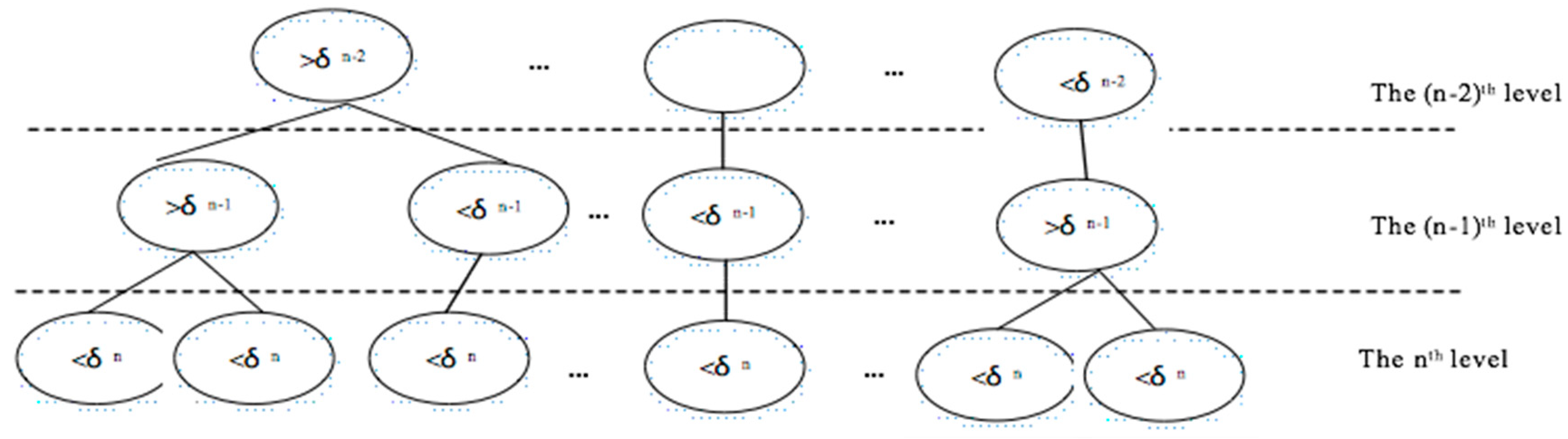
3.1.2. Construction of Multilevel Point Clusters

Although the initial segmentation can divide some of the aggregated points into point sets to a certain extent, some point sets still include multiple ground objects (as shown in the red circle in Figure 3). In order to obtain higher-discrimination features of the point sets, and assign a semantic label to the laser point well, the initial point sets are further divided so that a point set only contains one ground object or part of a ground object. As a normalized cut [42] can effectively segment the point sets, it is introduced to segment the initial point sets to further obtain content-sensitive multilevel point clusters. Firstly, a point set is divided into two parts by normalized cut, until the number of points in the set is less than a predefined threshold δ. Different thresholds δⁿ are set by different levels, so the point cloud is divided into point sets with different levels and sizes (as shown in Figure 4). Note that n is the level number, δⁿ = ηe^x, where η is an empirical parameter, it is set as 10, and x is an integer related with the level number. The formula of normalized cut is as follows:

$$Ncut\left(A,B\right)=\frac{cut\left(A,B\right)}{assoc\left(A,V\right)}+\frac{cut\left(A,B\right)}{assoc\left(B,V\right)}$$

(1)

where the V represents a point set, and A and B represent the two divided point sets, respectively. Subscript Ncut(A,B) represents the sum of the separated edge weights between two sets of points, the assoc(A,V) is the sum of the edge weights associated with all points in A, and assoc(B,V) represents the sum of the edge weights associated with all points in B.

3.2. Feature Construction of Content-Sensitive Multilevel Point Clusters

After the generation of content-sensitive multilevel point clusters, the features of the content-sensitive multilevel point clusters are extracted. As the point-based features are the basis of constructing the features of point clusters, these features in each point cluster are extracted first. Sparse coding and LDA joint learning are then used to express the features of multilevel point clusters on the basis of point features.

3.2.1. Extraction of the Point-Based Features

The method described in [39] is used in this study to extract point-based features. This method mainly extracts geometric features by using spatial 3D geometric information. It first determines the optimal size of the local 3D neighborhood of each point, which can increase the distinctiveness of features. The 3D features are then extracted based on the neighborhood. In addition, some extra information or specific structures will be revealed when projecting the 3D point cloud onto the horizontally-oriented plane. Following this, more features are extracted based on 2D projections. Finally, 26-dimensional feature descriptors are extracted for each point, which are listed as follows: the absolute height (z) of the single point, the range radius (r) of the local 3D neighborhood, the local point density (D), the verticality (V) (vertical component based on the single-point local normal vector), the maximum height difference (ΔZ) of the points in the neighborhood, the standard deviation (σ_Z) of the height value, the normalized eigenvalues e₁, e₂, and e₃ of the 3D structure tensor, characteristics of vectorized calculation based on eigenvalues (linearity L_λ, planarity P_λ and scattering S_λ, omnivariance O_λ, anisotropy A_λ, and eigenentropy E_λ), sum of the three eigenvalues Σ_λ, local surface change C_λ, radius of 2D neighborhood range (r_2D) after 2D projection, local point density D_2D, the two eigenvalues of 2D structure tensor, sum of two eigenvalues Σ_λ,2D, the ratio of the two value R_λ,2D, the number (M) of points falling in the 2D bin, the maximum height difference (Δz) of the points in the 2D box, and the standard deviation (σ_z) of the height value.

3.2.2. Feature Construction of Multilevel Point Clusters by Sparse Coding and LDA

In image processing, the BoW method [43] is generally used to quantize each extracted key point into words, then the image is represented by the histogram of the words to obtain a high level of classification or recognition effect. Inspired by the BoW method, sparse coding is introduced to describe the features of point clusters in this method. Sparse coding has obvious advantages in dictionary extraction and feature expression [44], and is based on the basic assumption that input data can be represented by a linear combination of words in an overcomplete dictionary, which can be obtained through point-based feature training. Firstly, a point set is defined as a document, and all point sets constitute a set of documents. The dictionary obtained by sparse coding is then defined as a dictionary of LDA. Following this, each point-based feature in the point set is used as basic unit, and sparse coding is utilized to express the features of points. In each point set, the frequency of each word is calculated to generate a word frequency vector with length V, where V represents the number of words in the dictionary. The SC-LDA (sparse coding-LDA) model is used, which is trained by point-based features to extract the probability of each latent topic in the point set. Finally, the vector F_SL, formed by the probability, acts as the feature of the point set [24].

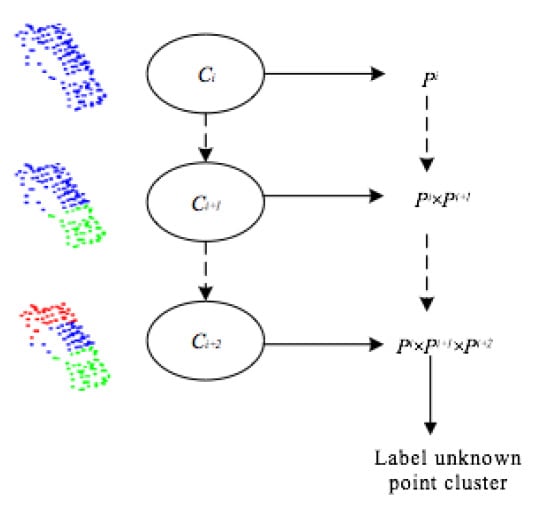
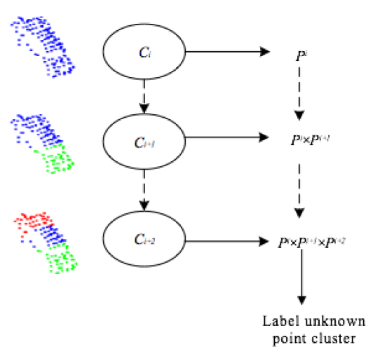
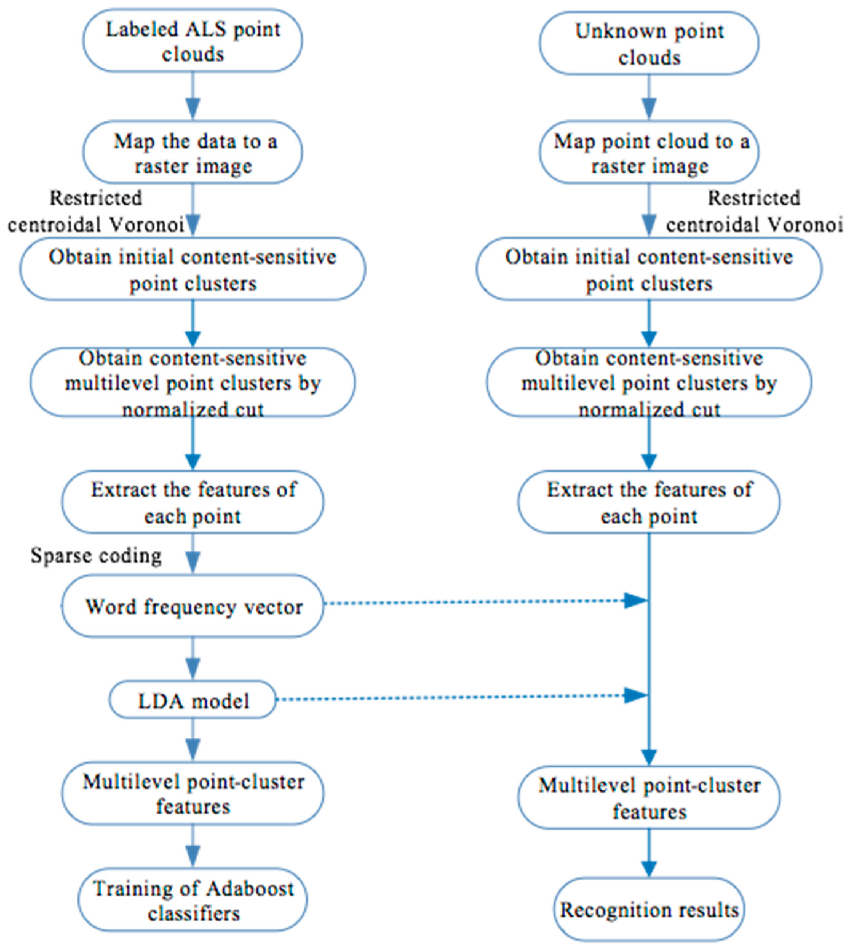
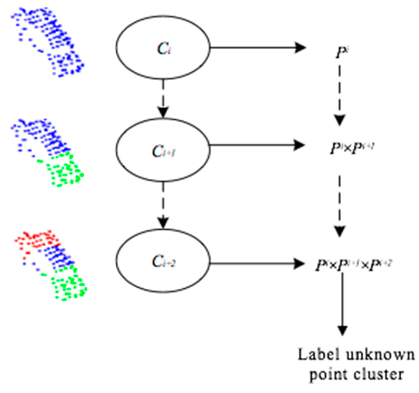
3.2.3. Hierarchical Framework of Point Cloud Classification

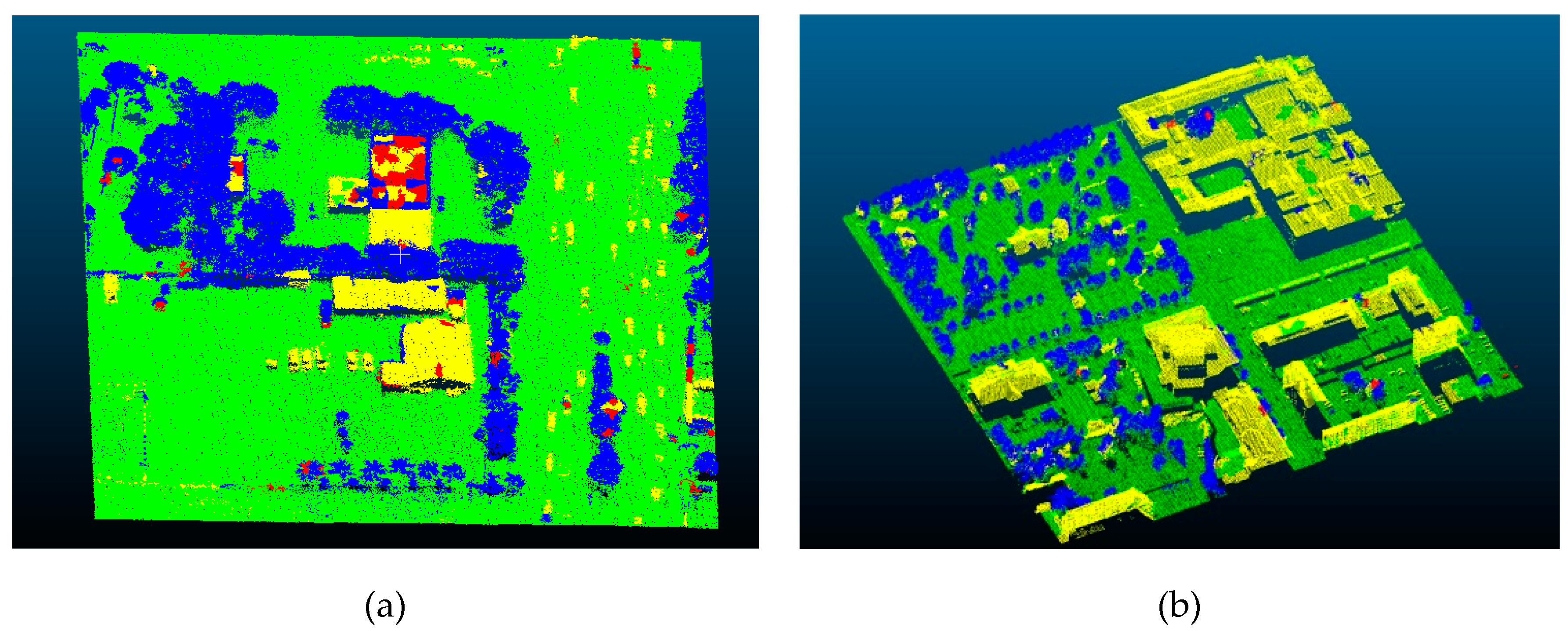
With the aid of the AdaBoost classifier, the multilevel point-clusters features obtained in Section 3.2.2 are used to generate a hierarchical classification framework. In the training process, the training data is initially clustered into multilevel point clusters, then multilevel point-cluster features based on the SC-LDA model are extracted. Following this, the AdaBoost classifiers of each class at each level are obtained through training. It is assumed that the ground objects are divided into four categories: buildings, trees, ground, and cars. The training data is divided into n-layer point clusters, and 4×n AdaBoost classifiers are trained. The SC-LDA model parameters and AdaBoost classifiers are obtained successively, then the trained classifiers are used for the identification of unmarked point clouds. In the process of identifying the unknown point cloud (the test process), the point cloud is first aggregated into content-sensitive multilevel point clusters, then the multilevel point-cluster features based on the SC-LDA model are extracted. Next, the trained classifiers are used for identification and classification. In the classification process, a method (Method III in Section 5) that eliminates hierarchical structure is also implemented to demonstrate the superiority of the proposed technique, which utilizes the initial segmented point sets by using a content-sensitive process to obtain classification results by the SC-LDA model. As shown in Figure 5, the probability that the i^th hierarchical point cluster C_i is marked as l_i is Pⁱ, the probability that the (i+1)^th-level point cluster C_i+1 is marked as l_i is Pⁱ⁺¹, and the probability that the (i+2)^th-level point cluster C_i+2 is marked as l_i is Pⁱ⁺². On the basis of inheriting the recognition result of the previous hierarchical point set C_i, the probability that the point cluster C_i+1 is marked as l_i is Pⁱ×Pⁱ⁺¹. Similarly, the probability that the point cluster C_i+2 is marked as l_i is Pⁱ × Pⁱ⁺¹ × Pⁱ⁺². Thus, the probability that a point cluster will eventually be marked as the label l_i can be expressed mathematically as:

$$P_n^j\left(l_i\right)={\displaystyle \prod }_{m=1}^n{P}^{m,num}\left(l_i,F_{SL}\right)$$

(2)

where n represents the total number of levels of the multilevel point clusters, $P_n^j$ is the probability that the j^th point cluster belongs to the category l_i, $P^{m,num}$ represents the probability that the m^th point cluster in the num^th hierarchical point cluster belongs to the category l_i, and $F_{SL}$ is the feature obtained by each point cluster based on the SC-LDA model. Finally, all point clusters in the top level are labeled by the highest probability of the labels.

4. Results

To verify the performance of the proposed method, point clouds from two urban scenes are used for qualitative and quantitative evaluation and analysis. In this section, the experimental datasets are introduced, and experimental results with experimental datasets are presented and analyzed. Finally, the sensitivities of the parameters in the method are tested, and error analysis is carried out.

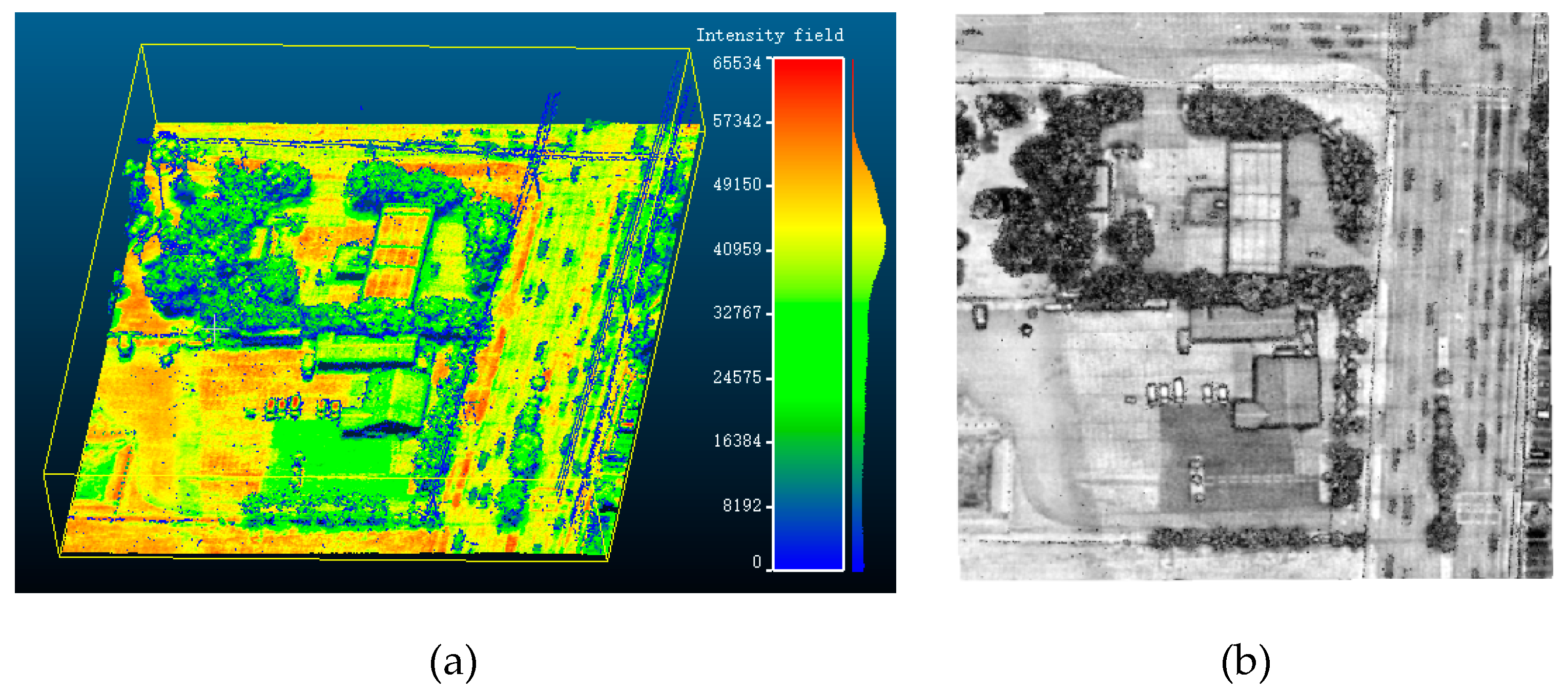
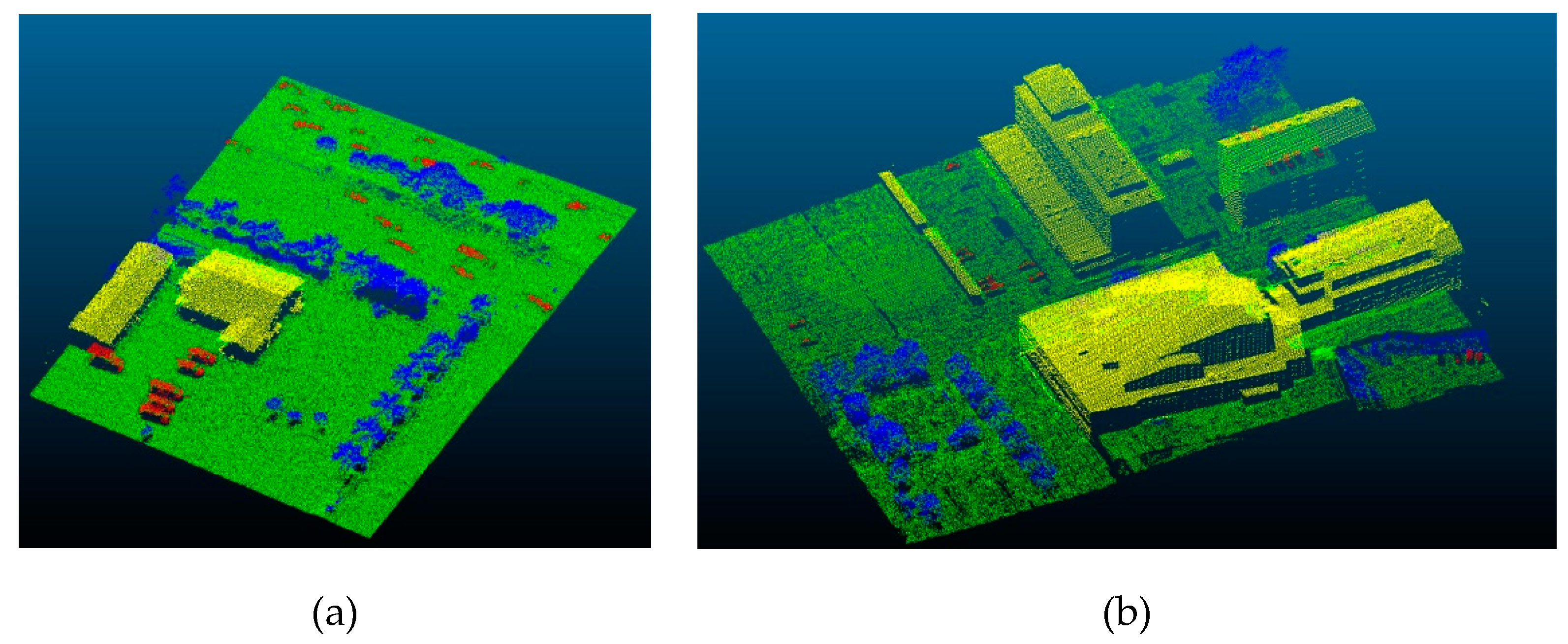
4.1. Experimental Datasets

Two different datasets (Scene I and Scene II) are captured in this study. Scene I contains 775,531 points with an average density of 3 points/m², and the area size is 510 m × 460 m. Scene II contains 819,999 points with an area size of 290 m by 320 m, and an average density of 8 points/m². The outliers of point clouds in the two scenes are few, and there are some differences in the density of the scenes. Objects such as buildings, trees, and cars are present in both experimental scenes. Buildings with different roof shapes, such as flat tops and spires, are surrounded by trees and cars in Scene I. In Scene II, there are buildings with different heights, dense trees with varying heights, and parked cars. Scenes I and II are both used to validate the proposed method.

Points from each scene are selected to form the training datasets (as shown in Figure 6).

Table 1. Experimental datasets.

	Point Number of the Training Data				Point Number of the Test Data
	Trees	Ground	Buildings	Cars	Trees	Ground	Buildings	Cars
Scene I	33,882	143,907	15,587	5939	217,869	453,102	32,153	12,407
Scene II	22,836	76,816	70,808	882	171,657	337,478	305,625	5239

lists the number of training points and test points in the two scenes. Taking the typicality of the training samples into account, the training data includes buildings with different heights, and trees with different densities. All points in Scenes I and II are used as experimental test datasets, and the number of points in each category are also listed in Table 1.

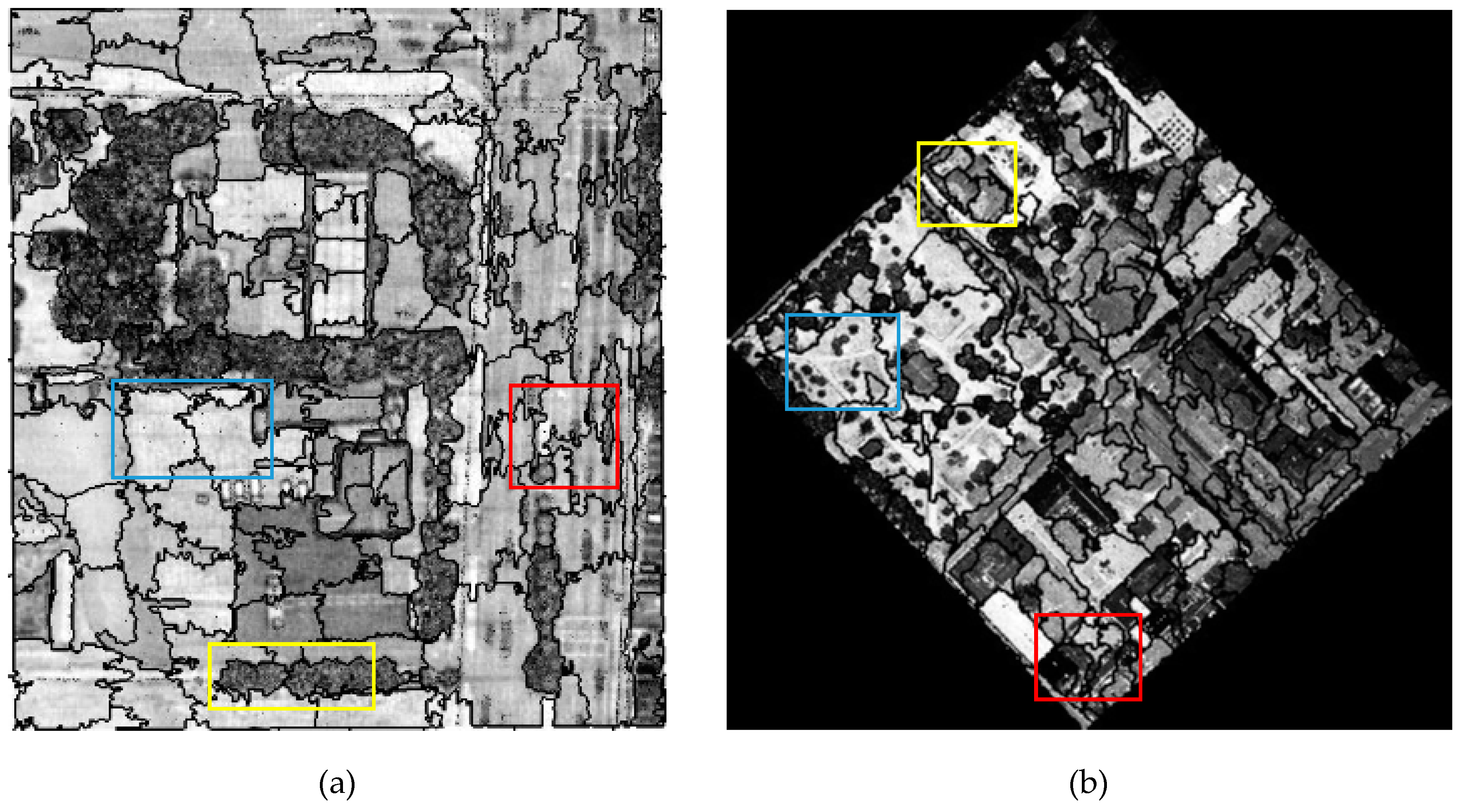
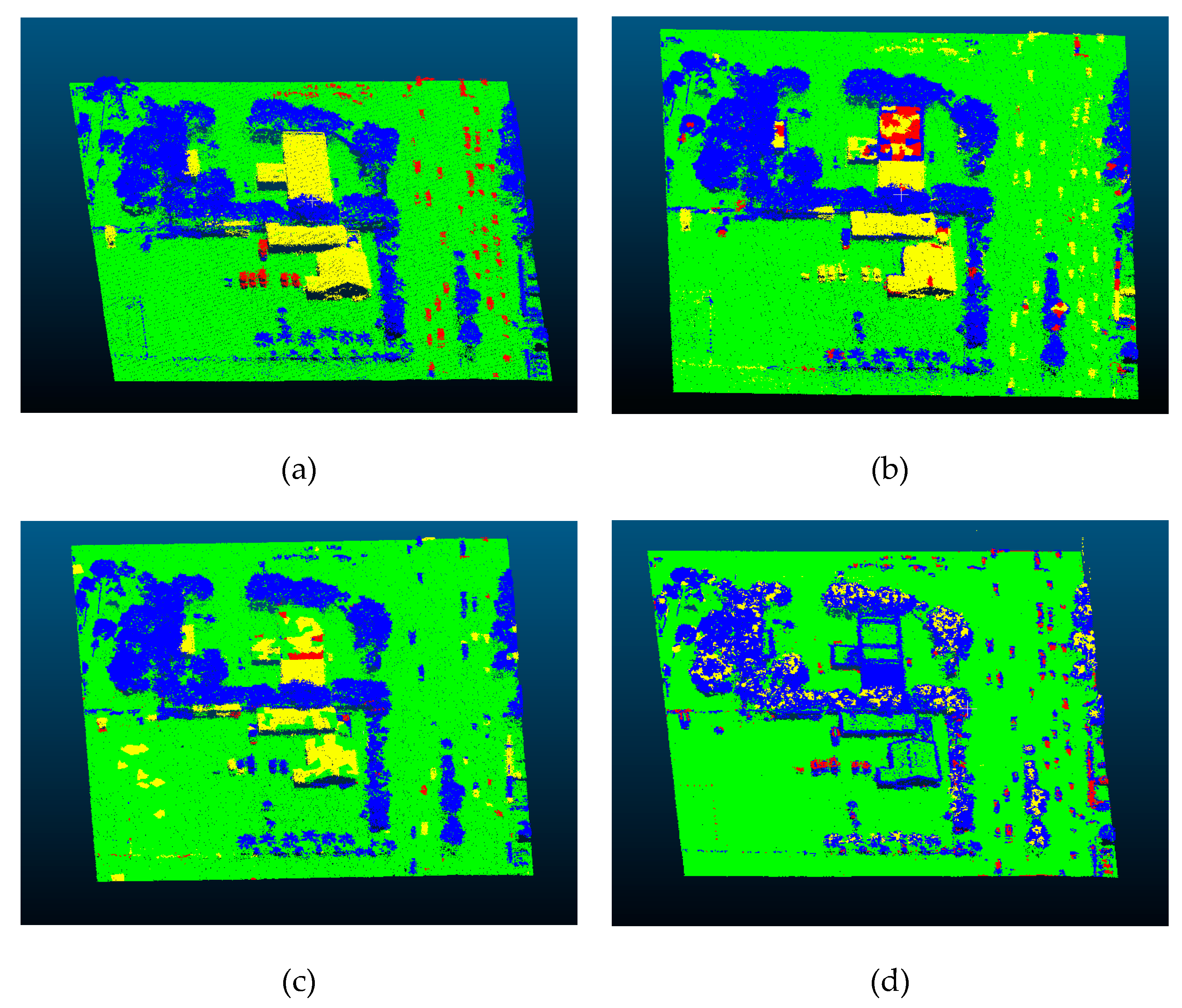
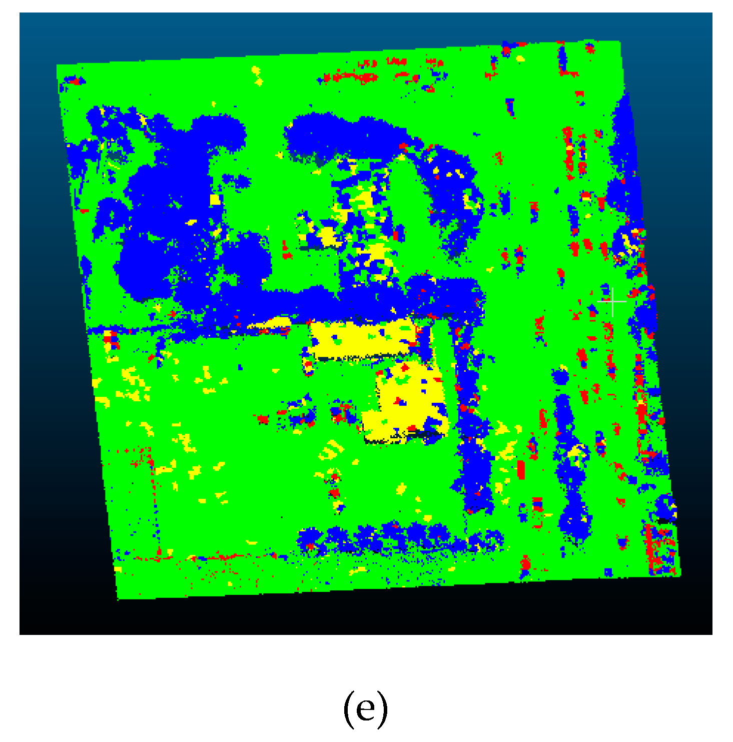
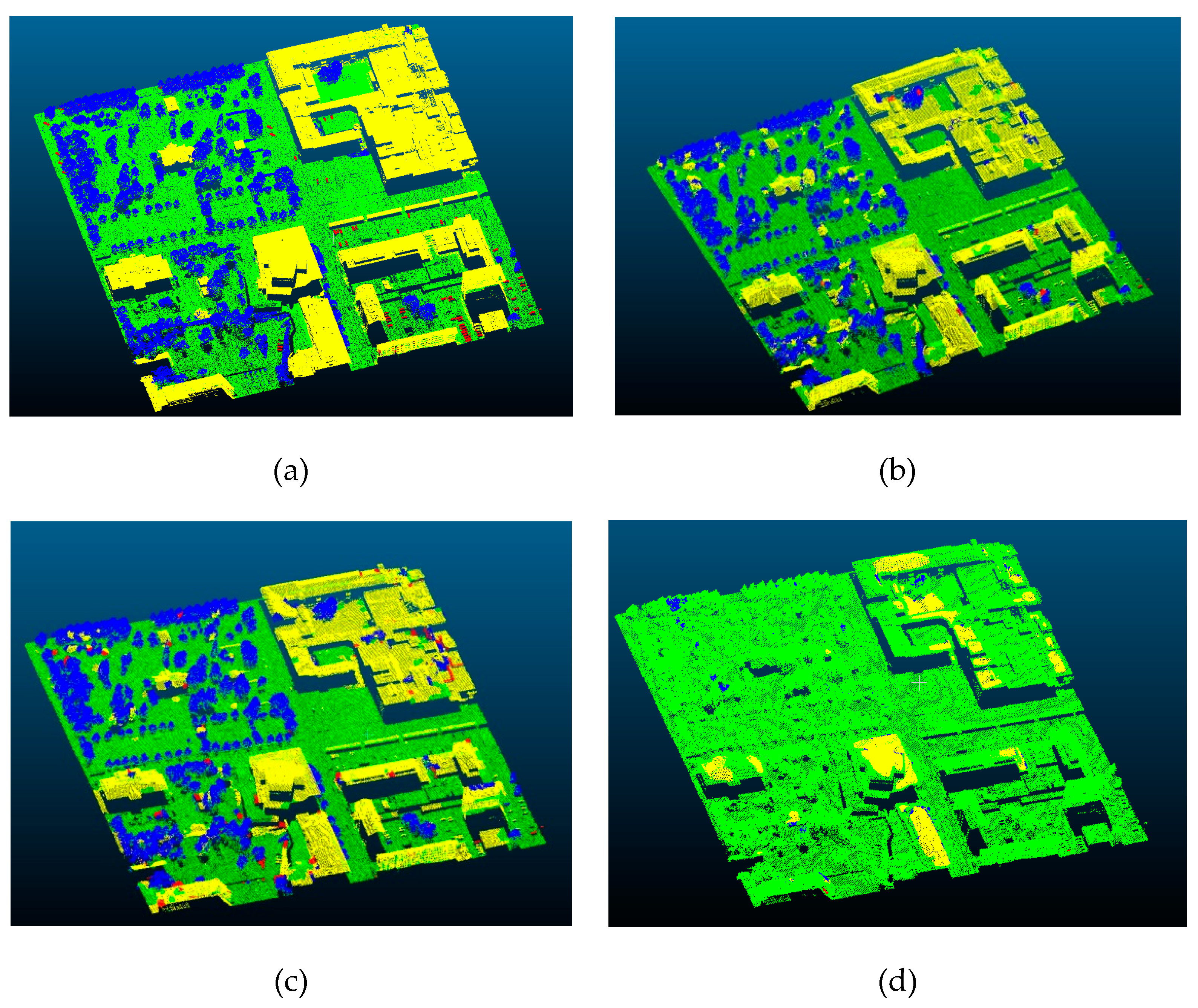
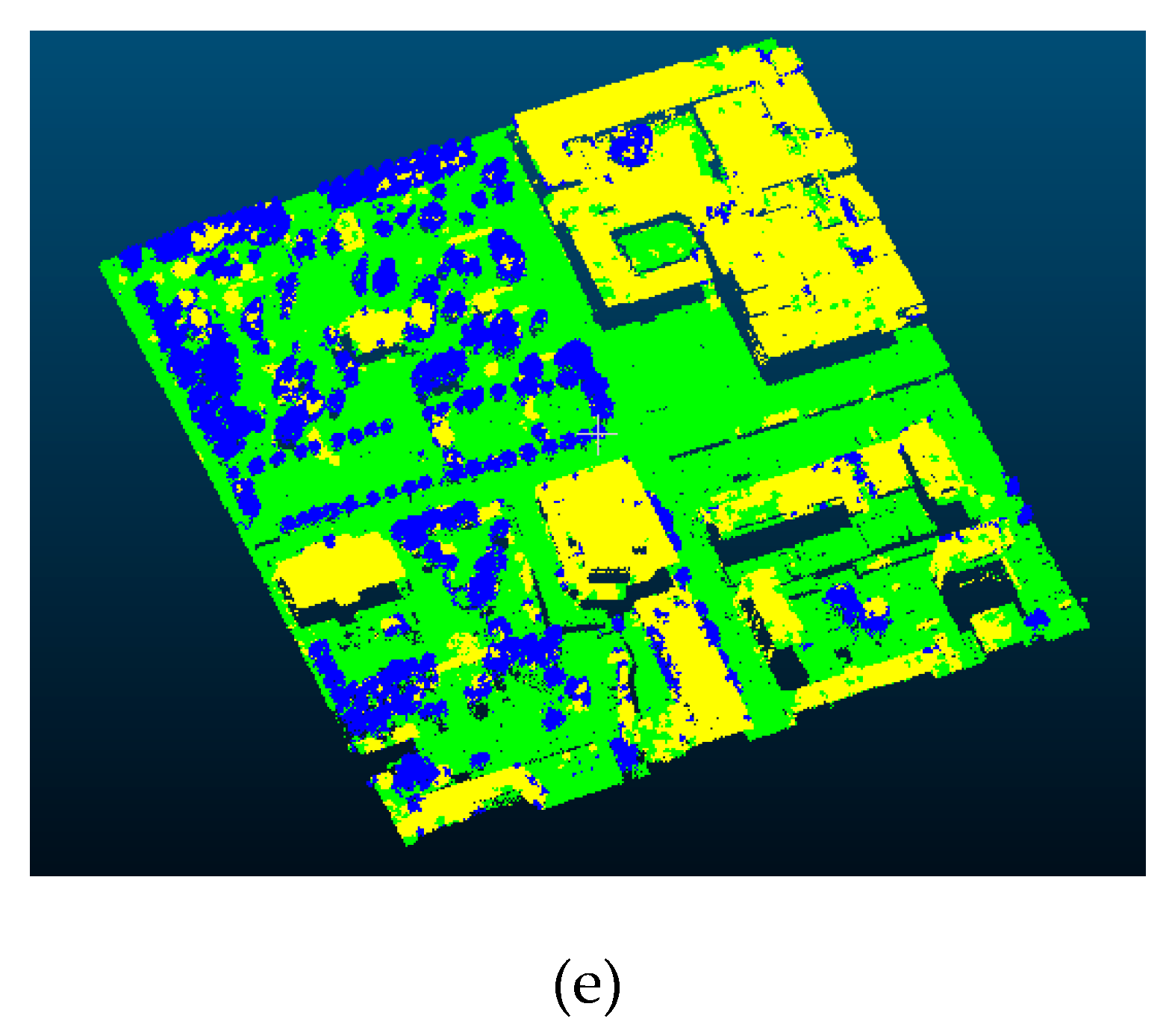
4.2. Experimental Results and Analysis

In the process of constructing initial content-sensitive point sets, superpixel results are obtained, as shown in Figure 7. Small point sets appear in content-dense areas, as shown in the blue rectangle, and large sets are generated in content-sparse areas, as shown in the red rectangle in Figure 7. The edges of building and trees are segmented, illustrated by the yellow rectangle, indicating that the content-sensitive method can sense the densities of the object distribution and hierarchies of spatial structure, and the content-sensitive hierarchical point clusters adapt the contents of the ground objects.

Precision-recall can be used to assess the quality of the classification. Precision is the fraction of relevant instances among the retrieved instances, while recall (also known as sensitivity) is the fraction of relevant instances that have been retrieved over the total amount of relevant instances. High precision means that the results returned by an algorithm are much more relevant than unrelated results, whereas high recall means that an algorithm returned most of the relevant results.

Table 2. Precision-recall and accuracy of different scenes.

	Tree (%)	Ground (%)	Building (%)	Car (%)	Accuracy (%)
Scene I	96.92/95.35	99.23/99.93	61.24/65.04	6.04/5.23	95.29
Scene II	96.54/84.22	96.7/94.09	85.02/94.44	9.72/4.2	91.60

shows the precision-recall and accuracy of the proposed method in the test stage, and Figure 8 illustrates the classification results of the two scenes. Most of the points are correctly identified by the method, except for some buildings and indistinguishable cars, as shown in Figure 8. Table 2 shows that the precision-recall of the tree and ground are high in both scenes. The precision-recall of the cars is not high enough in both scenes, because the cars are small, and the points are few, resulting in classification difficulties. The precision-recall of buildings is high in Scene II, but not high enough in Scene I. This is because the materials of various building roofs may be different, which has an impact on the training and test results. The roof material of Scene I is more diverse, so the precision-recall of buildings is not high enough.

4.3. Sensitivities of Parameters

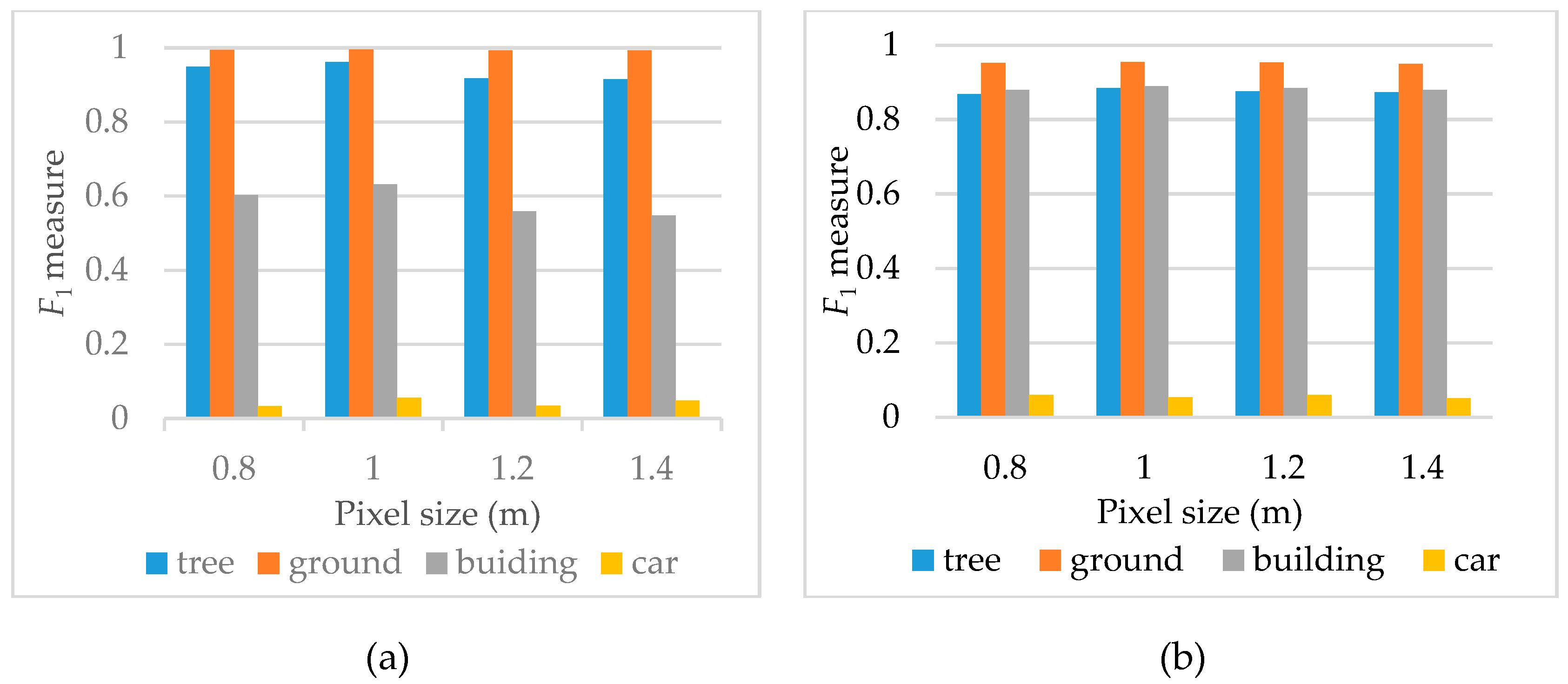
In this section, the influences of several important parameters in the process of the construction of content-sensitive multilevel point clusters on the classification accuracy are tested. This includes the pixel size p in the process of mapping point cloud to image, the number of superpixels K in the superpixel clustering process, the ratio of the training data to total data (s), and the density of resampled point cloud (d). The F₁ measure (Equation (3)) is used to represent the classification quality of Scenes I and II [26]:

$$F_1=\frac{2\left(recall\times precision\right)}{recall+precision}$$

(3)

4.3.1. Pixel Size

In order to test the effects of different pixel sizes (p) on the classification results, various p values are set to obtain different classification results. The p values are set respectively as 0.8 m, 1.0 m, 1.2 m, and 1.4 m, the number of superpixels K is 300, s value is 25%, and d value is 100%. The test results are provided in Figure 9. In Scene I, the F₁ measure values of tree and ground recognition for the proposed method both exceed 0.9. In Scene II, the F₁ measure value for ground recognition exceeds 0.9, and the F₁ measure values for building and tree identification are close to 0.9. From the trend of F₁ measure values of the four ground objects in the two scenes, the method maintains the recognition stability of the four types of ground objects. When the value of p is 1 m, the four types of ground objects in both scenes can obtain superior F₁ measure values.

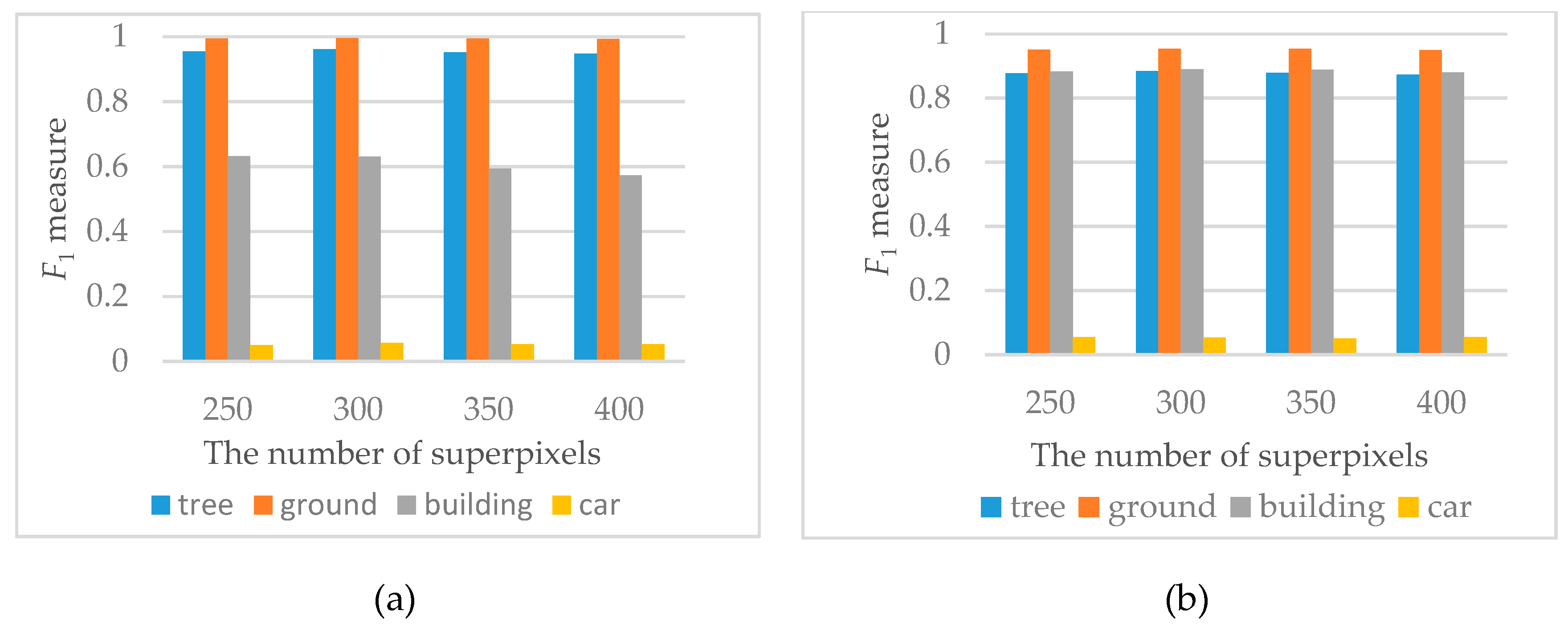
4.3.2. Effects of Superpixel Number

The K values are set as 250, 300, 350, and 400, p value is 1 m, athe s value is 25%, and the d value is 100%. The test results are provided in Figure 10. As illustrated, the F₁ measure values of Scene I for tree and ground recognition both exceed 0.9 at different K values. The F₁ measure value for ground recognition in Scene II also exceeds 0.9, and the F₁ measure values for tree and building identification are close to 0.9. From the trend of the F₁ measure values of the four ground objects in the two scenes, the method maintains the recognition stabilities of the four types of ground objects. When the K value is 300, the four types of ground objects in the scene can obtain better F₁ measure values, that is, superior recognition results can be acquired.

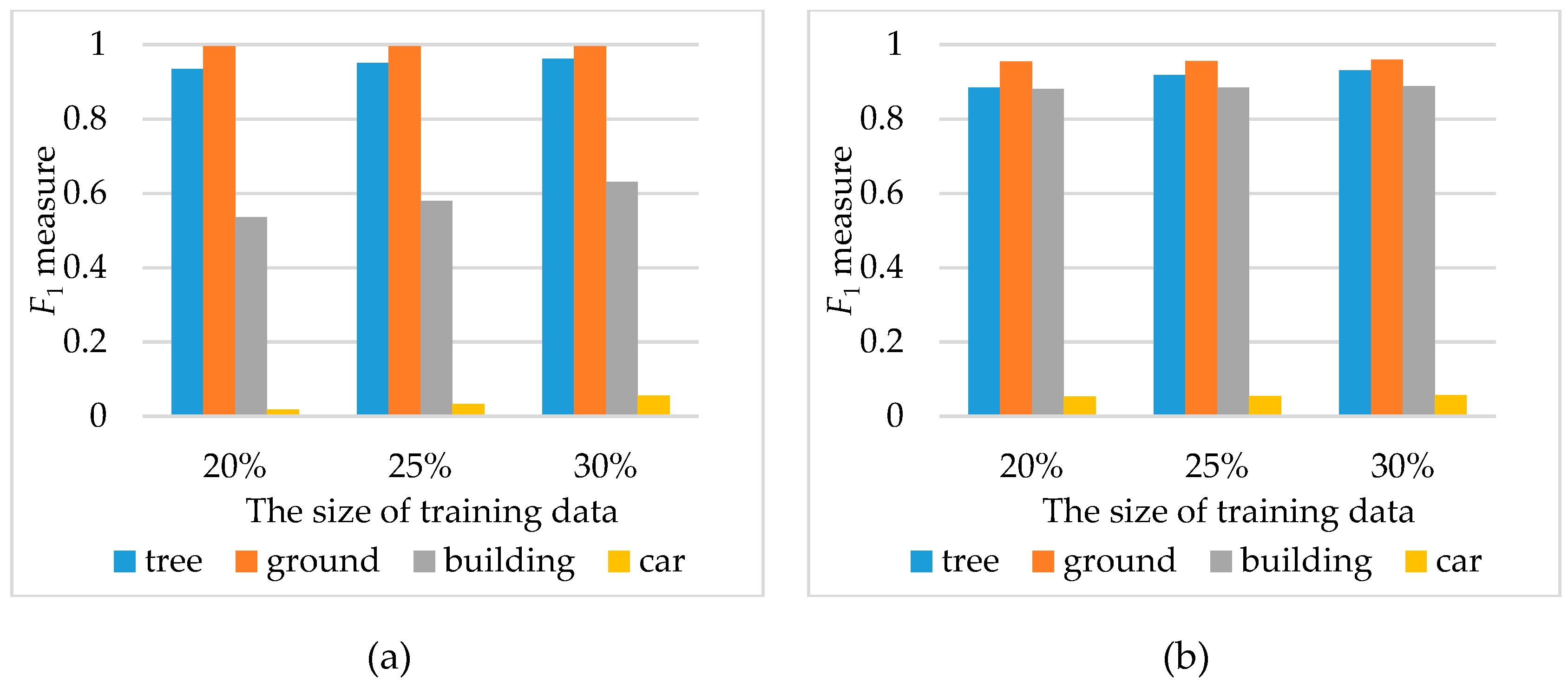
4.3.3. Ratio of the Training Data to Total Data (s)

To test the effects of training data, the s values are set as 20%, 25%, and 30%, which is the percentage of training data in the total data (test data). The p value is set as 1 m, K value as 300, and d value as 100%. The test results are provided in Figure 11. From the trend of the F₁ measure values of the four ground objects in the two scenes, it can be determined that as the size of training data increases, the method is robust for the classification of the four on-ground objects.

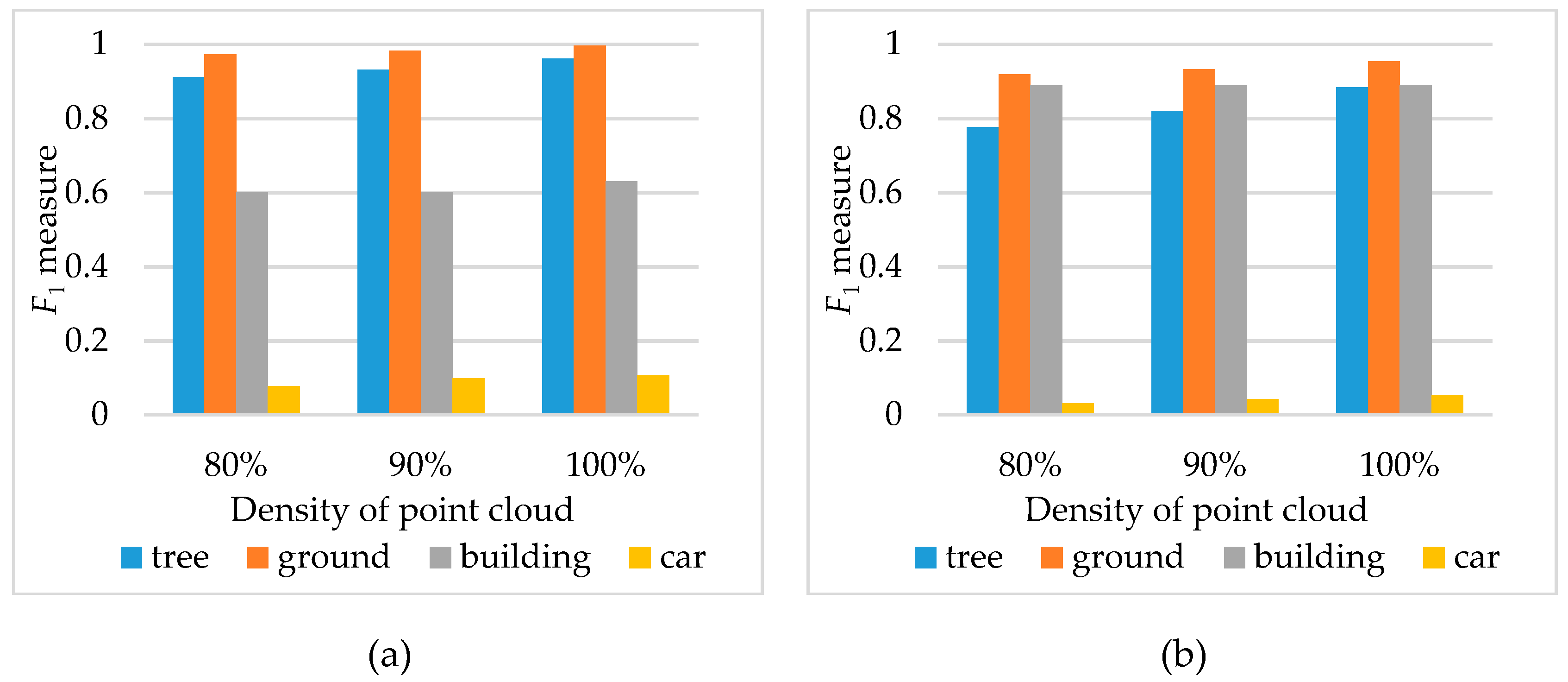
4.3.4. Density of the Point Cloud

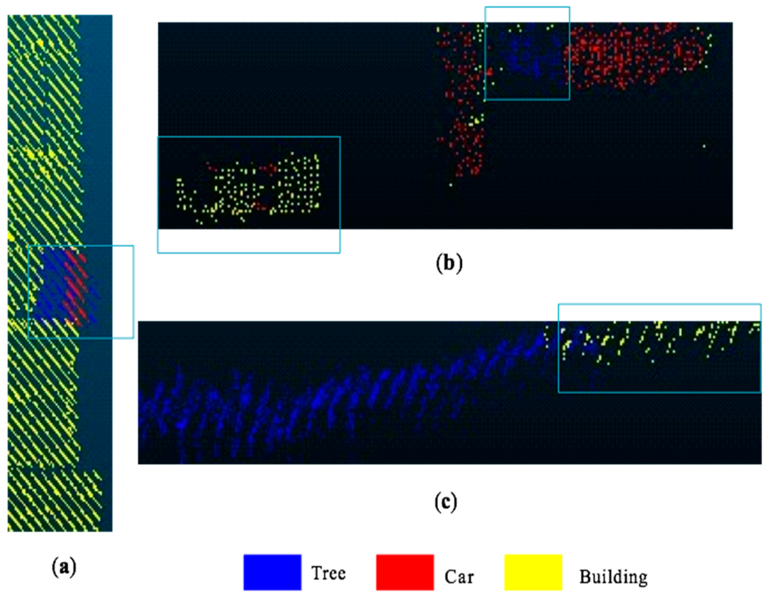
To test the influences of different densities of point clouds, the original data (d values) is randomly resampled as 80%, 90%, and 100%, which is the percentage of point cloud density to the original point cloud density. The p value is set as 1 m, K value as 300, and s value as 25%. The test results are shown in Figure 12. From the trend of the F₁ measure values of the four ground objects in the two scenes, it can be seen that as the density of the point cloud increases, and the F₁ measure values remain stable for the four kinds of objects.

4.4. Error Analysis

The classification results of Scene I are analyzed under the condition of p = 1, K = 300, s = 25%, and d = 100%, and Scene II under the condition of p = 1, K =300, s = 20%, and d = 100%.

Table 3. Confusion matrix of the classification results in Scene I.

	Tree	Ground	Building	Car	Recall
Overall Accuracy	95.29%
Tree	207,013	1449	3592	5044	0.9535
Ground	0	446,350	216	80	0.9993
Building	5888	354	20,869	4973	0.6504
Car	695	1661	9402	649	0.0523
Precision	0.9692	0.9923	0.6124	0.0604

and

Table 4. Confusion matrix of the classification results in Scene II.

	Tree	Ground	Building	Car	Recall
Overall Accuracy:	91.07%
Tree	138,335	0	29,606	1497	0.8164
Ground	0	316,857	19,888	0	0.9409
Building	5027	10,637	286,741	1230	0.9444
Car	93	188	4640	216	0.0420
Precision	0.9643	0.9670	0.8412	0.0734

list the confusion matrices of the two scenes. As shown in the rectangle of Figure 13a, the points on the prominent building eaves are often mistakenly classified into cars and trees, which is due to the limitation of techniques of scanning on-ground objects, resulting in uneven distribution of point clouds. Some car points are scattered, so that they are often incorrectly identified as buildings or trees (Figure 13b). For some trees, the point cloud distribution is relatively flat and similar to the roof of a building, so they are often misjudged as a building (Figure 13c). Despite such errors, the proposed method still identifies most of the points (as shown in Table 3 and Table 4, the total accuracy is 95.29% and 91.07%).

5. Discussion

To verify the performance of the proposed method it is compared with three other methods. The first method (Method I) uses the graph cut method and the SC-LDA model to classify the unknown data [24]. The graph cut method is used first to obtain the initial point clusters, multilevel segmentation is then implemented, and the features of multilevel point clusters are extracted using sparse coding and LDA models to carry out classification. However, this method does not take the density of the ground objects distribution into account. The second method (Method II) utilizes point-based classification [9], using the point-based method to directly extract single-point features, then employing the AdaBoost classifier to classify point clouds. This method does not aggregate data into point clusters or refer to hierarchical structures however. The third method (Method III) is defined in Section 3.2.3, and only uses the initial segmented point sets to obtain classification results, without constructing multi-level point clusters.

Table 5. Precision/recall and accuracy of different methods.

Scene I	Tree(%)	Ground(%)	Building(%)	Car(%)	Accuracy(%)
Proposed method	96.92/95.35	99.23/99.93	61.24/65.04	6.04/5.23	95.29
Method I	96.53/94.4	95.18/99.18	69.39/53.67	11.5/4.25	94.18
Method II	87.15/79.75	94.65/99.24	0.045/0.044	38.91/30.64	87.74
Method III	92.80/93.48	96.76/97.97	63.60/49.22	44.21/49.08	93.17
Scene II	Tree(%)	Ground(%)	Building(%)	Car(%)	Accuracy(%)
Proposed method	96.54/84.22	96.7/94.09	85.02/94.44	9.72/4.2	91.60
Method I	94.36/89.11	96.14/92.24	85.98/91.33	2.31/4.21	90.70
Method II	69.47/4.50	45.22/97.17	88.38/24.13	23.51/1.35	49.93
Method III	91.60/82.71	89.91/94.02	84.87/86.62	7.69/0.19	88.31

shows precision/recall and accuracy of the four methods during the test phase. As illustrated, the precision and recall of the classification results obtained by the proposed method are almost the highest in the four specific categories. In addition, the final classification accuracy of the method is higher than the other three techniques. Figure 14 and Figure 15 visually illustrate the classification results of the different methods, in which most of the points are correctly identified by the proposed method, except for some buildings and indistinguishable cars. As shown in Table 5, the classification results of Method II are the worst, which indicates that classification based on the point cluster is better than the single point. The accuracy of the classification results obtained by the proposed method is higher than Method III, and the precision-recall is almost higher than Method III in the four specific categories, indicating that classification based on the multilevel point clusters will achieve better results. The recognition of trees, ground, and buildings is superior to car identification using the method put forward in this paper and Method I, and the proposed method is superior or similar to Method I in identifying various types of ground objects. As the proposed technique can perceive the density variation of the ground object distribution, the constructed multilevel point clusters can adapt to the densities of the objects, and the features of the objects can be expressed more efficiently.

6. Conclusions

The point cloud classification method based on the content-sensitive multilevel point clusters was the focus of this study. The initial content-sensitive point sets of point cloud was first investigated, which takes the object entity content into account, and the initial classification unit was adapted to the densities of the ground objects. Secondly, the normalized cut method was used to segment the initial point set to construct content-sensitive multilevel point clusters. The point-based features of each hierarchical point cluster were then extracted, and the multilevel point-cluster features were constructed by sparse coding and LDA models. Finally, AdaBoost classifiers were used for training, and the prediction and recognition of the point cloud were completed based on the trained classifiers. Experiments were performed on point clouds in different scenes, and compared with three other methods. Most of the points were correctly identified by the proposed method, with an exception of some buildings and indistinguishable cars in the experimental results, and the accuracy of the proposed method was found to be superior to other state-of-the-art methods. At the same time, the setting of the parameters in the proposed method was determined to have little influence on the classification performance, meaning that the method is robust in recognizing different point clouds.

The two contributions in this framework are the construction of content-sensitive hierarchical point clusters, which can adapt the contents of the ground objects and hierarchies of spatial structure. Thus, the segmented hierarchical point clusters can achieve better construction of multilevel objects. In addition, a hierarchical classification framework based on content-sensitive hierarchical point clusters was designed, which can fully exploit spatial multilevel structures to accurately label unknown point clusters.

Future research will focus on improving the efficiency of this method and integrating point cluster-based deep feature into the framework.

References

1. Polewski, P.; Yao, W.; Heurich, M.; Krzystek, P.; Stilla, U. Detection of fallen trees in ALS point clouds using a normalized cut approach trained by simulation. ISPRS J. Photogramm. Remote Sens. 2015, 105, 252–271. [Google Scholar] [CrossRef]
2. Rodriguez-Cuenca, B.; Garcia-Cortes, S.; Ordonez, C.; Alonso, M.C. Automatic detection and classification of pole-like objects in urban point cloud data using an anomaly detection algorithm. Remote Sens. 2015, 7, 12680–12703. [Google Scholar] [CrossRef]
3. Wu, B.; Yu, B.; Wu, Q.; Huang, Y.; Chen, Z.; Wu, J. Individual tree crown delineation using localized contour tree method and airborne lidar data in coniferous forests. Int. J. Appl. Earth Obs. Geoinf. 2016, 52, 82–94. [Google Scholar] [CrossRef]
4. Garnett, R.; Adams, M.D. LiDAR—A Technology to Assist with Smart Cities and Climate Change Resilience: A Case Study in an Urban Metropolis. ISPRS Int. J. Geo-Inf. 2018, 7, 161. [Google Scholar] [CrossRef]
5. Serna, A.; Marcotegui, B. Urban accessibility diagnosis from mobile laser scanning data. ISPRS J. Photogramm. Remote Sens. 2013, 84, 23–32. [Google Scholar] [CrossRef] [Green Version]
6. Yang, B.; Dong, Z.; Liu, Y.; Liang, F.; Wang, Y. Computing multiple aggregation levels and contextual features for road facilities recognition using mobile laser scanning data. ISPRS J. Photogramm. Remote Sens. 2017, 126, 180–194. [Google Scholar] [CrossRef]
7. Golovinskiy, A.; Kim, V.G.; Funkhouser, T. Shape-based recognition of 3D point clouds in urban environments. In Proceedings of the IEEE International Conference on Computer Vision, Kyoto, Japan, 29 September–2 October 2009; pp. 2154–2161. [Google Scholar]
8. Guo, B.; Huang, X.; Zhang, F.; Sohn, G. Classification of airborne laser scanning data using JointBoost. ISPRS J. Photogramm. Remote Sens. 2015, 100, 71–83. [Google Scholar] [CrossRef]
9. Lodha, S.K.; Fitzpatrick, D.M.; Helmbold, D.P. Aerial Lidar Data Classification using AdaBoost. In Proceedings of the International Conference on 3-D Digital Imaging and Modeling, Montreal, QC, Canada, 21–23 August 2007; pp. 435–442. [Google Scholar]
10. Chehata, N.; Guo, L.; Mallet, C. Airborne Lidar Feature Selection for Urban Classification Using Random Forests. Available online: http://citeseerx.ist.psu.edu/viewdoc/download?doi=10.1.1.471.8566&rep=rep1&type=pdf (accessed on 31 January 2019).
11. Weinmann, M.; Jutzi, B.; Hinz, S.; Mallet, C. Semantic point cloud interpretation based on optimal neighborhoods, relevant features and efficient classifiers. ISPRS J. Photogramm. Remote Sens. 2015, 105, 286–304. [Google Scholar]
12. Tóvári, D. Segmentation Based Classification of Airborne Laser Scanner Data. Ph.D. Thesis, Universität Karlsruhe, Karlsruhe, Germany, 2006. [Google Scholar]
13. Darmawati, A. Utilization of Multiple Echo Information for Classification of Airborne Laser Scanning Data. Master’s Thesis, ITC Enschede, Enschede, The Netherlands, 2008. [Google Scholar]
14. Yao, W.; Hinz, S.; Stilla, U. Object extraction based on 3d-segmentation of lidar data by combining mean shift with normalized cuts: Two examples from urban areas. In Proceedings of the 2009 Joint Urban Remote Sensing Event, Shanghai, China, 20–22 May 2009; pp. 1–6. [Google Scholar]
15. Yang, B.S.; Dong, Z.; Zhao, G.; Dai, W.X. Hierarchical extraction of urban objects from mobile laser scanning data. ISPRS J. Photogramm. Remote Sens. 2015, 99, 45–57. [Google Scholar] [CrossRef]
16. Zhang, J.X.; Lin, X.G.; Liang, X.H. Research progress and prospects of point cloud information extraction. Acta Geodaetica et Cartographica Sinica. 2017, 46, 1460–1469. [Google Scholar]
17. Wang, Y.; Cheng, L.; Chen, Y.M.; Wu, Y.; Li, M.C. Building point detection from vehicle-borne LIDAR data based on voxel group and horizontal hollow analysis. Remote Sens. 2016, 8, 419. [Google Scholar] [CrossRef]
18. Zhang, J.X.; Lin, X.G.; Ning, X.G. SVM-based classification of segmented airborne lidar point clouds in urban areas. Remote Sens. 2013, 5, 3749–3775. [Google Scholar] [CrossRef]
19. Zhang, Z.; Zhang, L.; Tan, Y.; Zhang, L.; Liu, F.; Zhong, R. Joint discriminative dictionary and classifier learning for ALS point cloud classification. IEEE Trans. Geosci. Remote Sens. 2017, 56, 524–538. [Google Scholar] [CrossRef]
20. Liu, Y.J.; Yu, C.C.; Yu, M.J. Manifold SLIC: A Fast Method to Compute Content-Sensitive Superpixels. In Proceedings of the IEEE Conference on Computer Vision and Pattern Recognition (CVPR), Las Vegas, NV, USA, 27–30 June 2016; pp. 651–659. [Google Scholar]
21. Niemeyer, J.; Mallet, C.; Rottensteiner, F.; Sörgel, U. Conditional random fields for the classification of lidar point clouds. ISPRS Int. Arch. Photogramm. Remote Sens. Spat. Inf. Sci. 2011, 38, 209–214. [Google Scholar] [CrossRef]
22. Kim, H.B.; Sohn, G. Random forests based multiple classifier system for power-line scene classification. In Proceedings of the International Archives of the Photogrammetry, Remote Sensing and Spatial Information Sciences, Calgary, AB, Canada, 29–31 August 2011. [Google Scholar]
23. Lin, X.G.; Zhang, J.X. Multiple-primitives-based hierarchical classification of airborne laser scanning data in urban areas. ISPRS Int. Arch. Photogramm. Remote Sens. Spat. Inf. Sci. 2017, 42, 837–843. [Google Scholar]
24. Zhang, Z.; Zhang, L.; Tong, X.; Wang, Z.; Guo, B.; Huang, X. A multilevel point-cluster-based discriminative feature for ALS point cloud classification. IEEE Trans. Geosci. Remote Sens. 2016, 54, 3309–3321. [Google Scholar] [CrossRef]
25. Zhang, Z.; Zhang, L.; Tong, X.; Wang, Z.; Guo, B.; Zhang, L.; Xing, X. Discriminative-dictionary-learning-based multilevel point-cluster features for ALS point-cloud classification. IEEE Trans. Geosci. Remote Sens. 2016, 54, 7309–7322. [Google Scholar] [CrossRef]
26. Wang, Z.; Zhang, L.Q.; Tian, F.; Chen, D. A Multiscale and Hierarchical Feature Extraction Method for Terrestrial Laser Scanning Point Cloud Classification. IEEE Trans. Geosci. Remote Sens. 2015, 53, 2409–2425. [Google Scholar] [CrossRef]
27. Boykov, Y.; Veksler, O.; Zabih, R. Fast approximate energy minimization via graph cuts. IEEE Trans Pattern Anal Mach Intell. 2001, 23, 1222–1239. [Google Scholar] [CrossRef] [Green Version]
28. Shi, J.; Malik, J. Normalized cuts and image segmentation. IEEE Trans Pattern Anal Mach Intell. 2000, 22, 888–905. [Google Scholar] [Green Version]
29. Yokoyama, H.; Date, H.; Kanai, S.; Takeda, H. Detection and classification of pole-like objects from mobile laser scanning data of urban environments. Int. J. Cad/Cam. 2013, 13, 31–40. [Google Scholar]
30. Barnea, S.; Filin, S. Segmentation of terrestrial laser scanning data by integrating range and image content. In Proceedings of the XXIth ISPRS Congress, Beijing, China, 3–11 July 2008. [Google Scholar]
31. Comaniciu, D.; Meer, P. Mean Shift: A Robust Approach Toward Feature Space Analysis. IEEE Trans Pattern Anal Mach Intell. 2002, 24, 603–619. [Google Scholar] [CrossRef]
32. Barnea, S.; Filin, S. Segmentation of terrestrial laser scanning data using geometry and image information. ISPRS J. Photogramm. Remote Sens. 2013, 76, 33–48. [Google Scholar] [CrossRef]
33. Farabet, C.; Couprie, C.; Najman, L.; Lecun, Y. Learning hierarchical features for scene labeling. IEEE Trans Pattern Anal Mach Intell. 2013, 35, 1915–1929. [Google Scholar] [CrossRef] [PubMed]
34. Brodu, N.; Lague, D. 3D terrestrial lidar data classification of complex natural scenes using a multi-scale dimensionality criterion: applications in geomorphology. ISPRS J. Photogramm. Remote Sens. 2012, 68, 121–134. [Google Scholar] [CrossRef]
35. Pauly, M.; Keiser, R.; Gross, M. Multi-scale feature extraction on point-sampled surfaces. In Computer Graphics Forum; Blackwell Publishing, Inc.: Oxford, UK, 2003; pp. 281–289. [Google Scholar]
36. Xiong, X.; Munoz, D.; Bagnell, J.A.; Hebert, M. 3-d scene analysis via sequenced predictions over points and regions. In Proceedings of the IEEE International Conference on the Robotics and Automation (ICRA), Shanghai, China, 9–13 May 2011; pp. 2609–2616. [Google Scholar]
37. Xu, S.; Oude, E.S.; Vosselman, G. Entities and features for classification of airborne laser scanning data in urban area. In Proceedings of the XXII ISPRS Congress, Melbourne, VIC, Australia, 25 August–1 September 2012; pp. 257–2662. [Google Scholar]
38. Mallet, C. Analysis of Full-Waveform LIDAR Data for Urban Area Mapping. Ph.D. Thesis, Télécom ParisTech, Paris, France, 2010. [Google Scholar]
39. Weinmann, M.; Urban, S.; Hinz, S.; Jutzi, B.; Mallet, C. Distinctive 2D and 3D features for automated large-scale scene analysis in urban areas. Comput. Graph. 2015, 49, 47–57. [Google Scholar] [CrossRef]
40. Liu, Y.J.; Yu, M.; Li, B.J.; He, Y. Intrinsic manifold SLIC: A simple and efficient method for computing content-sensitive superpixels. IEEE Trans Pattern Anal Mach Intell. 2018, 40, 653–666. [Google Scholar] [CrossRef] [PubMed]
41. Liu, J.; Tang, Z.; Cui, Y.; Wu, G. Local competition-based superpixel segmentation algorithm in remote sensing. Sensors. 2017, 17, 1364. [Google Scholar] [CrossRef]
42. Nadarajah, S. An approximate distribution for the normalized cut. J. Math Imaging. Vis. 2008, 32, 89–96. [Google Scholar] [CrossRef]
43. Nowak, E.; Frédéric, J.; Triggs, B. Sampling strategies for bag-of-features image classification. In Proceedings of the 9th European Conference on Computer Vision, Graz, Austria, 7–13 May 2006; pp. 490–503. [Google Scholar]
44. Han, B.; He, B.; Sun, T.; Ma, M.; Shen, Y.; Lendasse, A. HSR: L1/2-regularized sparse representation for fast face recognition using hierarchical feature selection. Neural Comput Appl. 2016, 27, 305–320. [Google Scholar] [CrossRef]
Figure 1. Method flowchart.
Remotesensing 11 00342 g001
Figure 2. Mapping point cloud to raster image. (a) Original point cloud; and (b) the raster image based on intensity.
Remotesensing 11 00342 g002
Figure 3. Superpixel clustering result.
Remotesensing 11 00342 g003
Figure 4. An illustration of the three-level content-sensitive point clusters.
Remotesensing 11 00342 g004
Figure 5. Labeling unknown point clusters.
Remotesensing 11 00342 g005
Figure 6. Training datasets. Blue points represent trees, green points are ground, yellow points are buildings, and red points are cars. (a) Training dataset obtained from Scene I; and (b) training dataset obtained from Scene II.
Remotesensing 11 00342 g006
Figure 7. The results of superpixels from the two scenes. (a) The superpixels result from Scene I; and (b) the superpixels result from Scene II.
Remotesensing 11 00342 g007
Figure 8. Classification results of the two scenes. (a) Classification results of Scene I; and (b) classification results of Scene II.
Remotesensing 11 00342 g008
Figure 9. Impacts of different sizes of pixel on the classification results. (a) Influences of different sizes of pixel on the classification results in Scene I; and (b) influences of different sizes of pixel on the classification results in Scene II.
Remotesensing 11 00342 g009
Figure 10. Impacts of different numbers of superpixel on the classification results. (a) Influences of different numbers of superpixel on the classification results in Scene I; and (b) influences of different numbers of superpixel on the classification results in Scene II.
Remotesensing 11 00342 g010
Figure 11. Impacts of different ratios of training data to total data on the classification results. (a) Influences of different ratios of training data to total data on the classification results in Scene I; and (b) influences of different ratios of training data to total data on the classification results in Scene II.
Remotesensing 11 00342 g011
Figure 12. Impacts of different densities of resampled point cloud on the classification results. (a) Influences of different densities of resampled point cloud on the classification results in Scene I; and (b) influences of different densities of resampled point cloud on the classification results in Scene II.
Remotesensing 11 00342 g012
Figure 13. Typical misclassification errors. (a) Points on the building edge are misclassified as tree and car; (b) car points are misclassified as tree and building; and (c) tree points are misclassified as building.
Remotesensing 11 00342 g013
Figure 14. Classification results of Scene I. (a) Ground truth; (b) classification results of proposed method; (c) classification results of Method I; (d) classification results of Method II; and (e) classification results of Method III. The tree, ground, building, and car are respectively colored by blue, green, yellow, and red.
Remotesensing 11 00342 g014aRemotesensing 11 00342 g014b
Figure 15. Classification results of Scene II. (a) Ground truth; (b) classification results of proposed method; (c) Classification results of Method I; (d) classification results of Method II; and (e) classification results of Method III. The tree, ground, building, and car are respectively colored blue, green, yellow, and red.
Remotesensing 11 00342 g015aRemotesensing 11 00342 g015b