Separating Built-Up Areas from Bare Land in Mediterranean Cities Using Sentinel-2A Imagery

Abstract

In this research work, a multi-index-based support vector machine (SVM) classification approach has been proposed to determine the complex and morphologically heterogeneous land cover/use (LCU) patterns of cities, with a special focus on separating bare lands and built-up regions, using Istanbul, Turkey as the main study region, and Ankara and Konya (in Turkey) as the independent test regions. The multi-index approach was constructed using three-band combinations of spectral indices, where each index represents one of the three major land cover categories, green areas, water bodies, and built-up regions. Additionally, a shortwave infrared-based index, the Normalized Difference Tillage Index (NDTI), was proposed as an alternative to existing built-up indices. All possible index combinations and the original ten-band Sentinel-2A image were classified with the SVM algorithm, to map seven LCU classes, and an accuracy assessment was performed to determine the multi-index combination that provided the highest performance. The SVM classification results revealed that the multi-index combination of the normalized difference tillage index (NDTI), the red-edge-based normalized vegetation index (NDVIre), and the modified normalized difference water index (MNDWI) improved the mapping accuracy of the heterogeneous urban areas and provided an effective separation of bare land from built-up areas. This combination showed an outstanding overall performance with a 93% accuracy and a 0.91 kappa value for all LCU classes. The results of the test regions provided similar findings and the same index combination clearly outperformed the other approaches, with 92% accuracy and a 0.90 kappa value for Ankara, and an 84% accuracy and a 0.79 kappa value for Konya. The multi-index combination of the normalized difference built-up index (NDBI), the NDVIre, and the MNDWI, ranked second in the assessment, with similar accuracies to that of the ten-band image classification.

1. Introduction

Throughout history, the increase in population densities and the expansion of urban areas, especially in metropolitan cities, have changed the form of the Earth’s surface [1]. The rate of land cover/use (LCU) changes has increased in recent decades. Population growth leads to increases in water and energy consumption and causes land surface changes, which result in regional to global climate change and environmental degradation [2,3].

LCU changes that have occurred due to urbanization, deforestation, desertification, natural disasters, and intense agricultural practices, have greatly influenced climatic characteristics at the regional and global scale. Such changes generally result in increases of near-surface temperatures and formation of heat islands, which trigger other climatic phenomena [3,4,5,6]. Thus, there is a need for accurate, up-to-date, and periodical LCU maps to develop efficient decision-making mechanisms to cope with climate change and effectively manage and plan cities [3,4,7]. With the advances in satellite technologies, traditional methods have been mostly replaced by remotely-sensed data analysis to monitor LCU change [8,9]. The availability of free global and historical satellite imagery provides a valuable opportunity for mapping and monitoring LCU, constantly and effectively [10,11]. The separate or combined use of optical and SAR data provide valuable information about the physical characteristics of land surface; different analysis methods have been developed to determine different object types. Among these methods, image classification has become the most popular method for mapping LCU and its changes [12,13].

Lu and Weng, 2007, reviewed the classification algorithms and accuracy of several image classification studies. They reported that the classification accuracy was affected by several factors and these factors can be grouped as: (i) Use of advanced classification algorithms, such as Support Vector Machine (SVM), Random Forest (RF), and regression tree (CART); (ii) selection of multiple remote sensing features, such as multi-spectral, multi-temporal, or multi-sensor data fusion; and (iii) integration of additional data, such as topographic maps or soil maps [14].

The use of non-parametric classification algorithms, such as machine learning algorithms, decision trees and knowledge-based classifiers have increased [14]. Among these, SVMs, which use a set of related learning algorithms for classification, showed a superior performance, compared to traditional classification techniques such asmaximum likelihood, minimum distance, or parallelepiped classifiers [15,16,17]. SVM also provided better performance when applied to multi-index images than the Neural Network (NN) classifier and regression trees (CART) [18]. In a recent article, Maulik and Chakraborty summarized the recently developed advanced SVM-based classification approaches used in remote sensing studies. They concluded that SVM-based classification methods perform better in terms of accuracy, speed, and memory requirements, and can operate effectively and accurately in cases where training samples are limited, which is generally the case for satellite image classification problems. They also noted the constraints that should be considered in SVM, such as the need to appropriately define the kernel function, the representation efficiency of the training sample, and the consistency of statistical distributions between classes [19].

In most satellite image classification scenarios, higher accuracies (over 85%) are attained when the major land cover (LC) classes, such as vegetation, water, and urban classes are the concern [20,21]. Achieving high accuracies becomes challenging when the higher-level class definitions are the concern, due to the spectral and spatial similarities [22]. According to a survey done by Li et al., the classification accuracies achieved by supervised algorithms vary greatly, due to the number of training samples and proprieties of selected features for classification [23]. These findings indicate a feature selection problem that occurs regardless of the classification algorithm. An increased number of features, such as the image bands, generally improves the accuracy; however, it increases the amount of training samples required [24]. Considering the limited training sample availability in most conditions and the nonlinear response of the LCU classes across several bands, which is known as the “Hughes effect” [25], there is a need for a method to select a subset of relevant features from the original dataset to improve the classification process and achieve a dimension reduction [26].

One alternative to overcome the above-mentioned problem is to perform linear transformation methods (such as principal components analysis (PCA) and independent component analysis (ICA)), or nonlinear algorithms (such as locality adaptive discriminant analysis (LADA) and multiple marginal fisher analysis (MMFA)), to remove the correlations and higher-order dependences in the image bands and use the produced components as input data for classification, to simplify and improve the process. The linear methods have been widely applied on multispectral data, however, nonlinear methods are generally applied on hyperspectral test data or natural image-based applications, such as face recognition [27,28,29,30].

Spectral indices derived from satellite images can be used as an alternative data source for LCU characterization [31,32,33,34]. The characteristics of the reflected energy in different regions of the spectrum for a specific land property, can be utilized to produce various indices. Using the spectral indices for LCU mapping is an operational approach as it enables LCU mapping at a higher degree of accuracy, which is highly comparable to those from a complex interpretation of quantity [35,36]. Zha et al. [37], for the first time, introduced an automated index-based method for mapping the built-up regions.

Nevertheless, there is a significant drawback that should be considered when using spectral indices for LCU mapping. Some land features, such as water bodies and vegetation cover have very specific spectral reflectance characteristics, which facilitate the separation from other features, using spectral indices. However, it is challenging to detect built-up areas and effectively separate them from bare lands using a single index, due to similarities in the spectral characteristics. Confusion over, and misclassification of, built-up areas and bare lands is a problem, which can be partially addressed by the available built-up, index-based analyses [37,38,39]. Urbanized areas are composed of heterogeneous surfaces, including different artificial materials and natural areas, and therefore, exhibit a complex landscape characteristic, making it difficult to map all LCU classes using a single index [40].

The main objective of this research work was to propose a multi-index-based SVM classification approach, for mapping seven different LCU classes, in complex urban areas. The research focused on separating the built-up areas and bare lands, in addition to providing an accurate and reliable LCU map, in three densely urbanized metropolitan cities of Turkey, using the Sentinel-2A imagery. The method design comprised using a few sets of specific indices, each group of which highlighted a generalized LCU category—built-up regions, vegetation covers, and water bodies. For the built-up category, the existing built-up indices and the normalized difference tillage index (NDTI) were used as the first components of the multi-index dataset, and their performances were evaluated. For the vegetation cover determination, NDVI, the soil adjusted vegetation index (SAVI), and the red-edge-based normalized difference vegetation index (NDVIre) were evaluated as the second component. The normalized difference water index (NDWI) and modified normalized difference water index (MNDWI) were used to highlight the water bodies as the third component. Several combinations of spectral indices and the original satellite images were classified using the same training sample set and supervised SVM algorithm, as it has a non-parametric, machine-learning-based structure and because of its reported performance in supervised, pixel-based algorithms, mentioned above [15,16,17]. Accuracy assessment was performed using stratified random points to evaluate the performance of the multi-index approach and its possible advantages over the traditional classification of the original spectral bands. The proposed approach was developed with the Sentinel-2A image of the metropolitan city of Istanbul and applied to two independent regions located in the metropolitan cities of Ankara and Konya, in Turkey, to validate the common usage and effectiveness.

2. Study Area

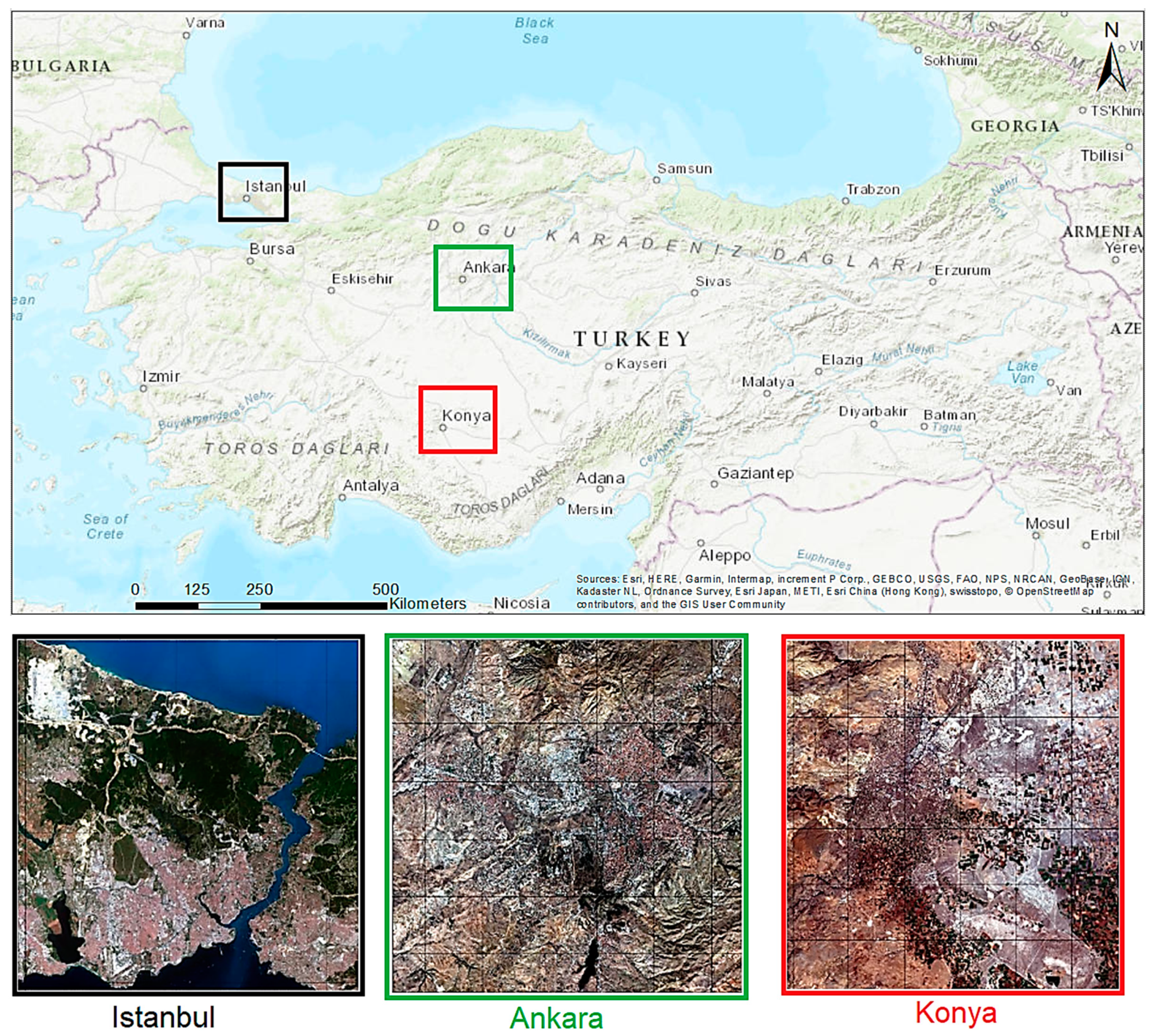
Istanbul is the most populated and the largest city in Turkey, located at a latitude of 41°00′44.06″ N and a longitude of 28°58′33.66″ E, in the Northern Hemisphere, joining the two continents of Asia and Europe. Istanbul is also one of the largest metropolitan cities of Europe, covering approximately 5.500 km², with a population over 15 million in 2017, corresponding to 18% of the country [41]. The significant population growth that occurred due to the industrial development and unplanned urbanization, during the second half of the twentieth century, resulted in critical transformations of the structure and morphology of the city. The densely urbanized regions of Istanbul are located in its southern half. In the last decade, construction of new transportation infrastructures, such as the Yavuz Sultan Selim Bridge, the Northern Black Sea Highway, and a third airport, have affected the ecosystem and caused a dramatic increase in built-up areas, in the northern half of the city. Istanbul presents a complex pattern of various feature classes, including forest, water bodies, croplands, bare land, and heterogeneous urban areas, making it a suitable candidate for the purpose of this research work.

The intensive urbanization in Istanbul and the change in LCU has attracted the attention of many researchers and several studies have been conducted to determine the LCU and its changes, using satellite images [42,43,44,45,46]. These studies have reported an intensive increase in urbanization—for different time-periods—that have resulted in the destruction of the natural landscape, by applying the traditional, pixel-based spectral image classification methods.

The two test regions, Ankara and Konya, are located in the middle of the country. Ankara is the capital of Turkey and is the second most crowded city after Istanbul. Konya is also an important city in Turkey, with a high level of industrial activity, which is ranked seventh in the urbanization rate. Both of these regions include high- and low-density residential areas and industrial areas that are located between and surrounded by extensive bare land, which makes them good candidates to test the challenging bare-land–urban-area separation process. The locations of the main study area and test regions have been presented in Figure 1.

3. Data

In this research, 1C-level-processed, cloudless Sentinel-2A images were used to perform the analysis and evaluation. The acquisition dates of the images were 29 June 2017, 3 November 2017, and 19 September 2018 for the Istanbul, Ankara, and Konya regions, respectively. The European Space Agency (ESA) developed the operational Sentinel-2 mission within the frame of the European Union Copernicus programme. The Sentinel-2 mission is based on a constellation of two satellites, Sentinel-2A and Sentinel-2B, flying in the same orbit but phased at 180°, to observe the land surface, thoroughly, with a short revisit period, and to meet the requirements of applications, such as land management, agriculture and forestry, and disaster control [47].

Sentinel-2A was launched on 23 June 2015 and was followed by Sentinel-2B on 7 March 2017; both maintain a sun-synchronous orbit at 786 km altitude. The temporal resolution is five days from the two-satellite constellations, at the equator. The multispectral imager covers 13 spectral bands with a swath width of 290 km and a spatial resolution of 10 m (four visible and near-infrared bands (NIR)), 20 m (six red-edge and shortwave infrared bands (SWIR)), and 60 m (three atmospheric correction bands). Sentinel-2 image products are available to the community at the Level-1C (top-of-atmosphere reflectance in cartographic geometry) and Level-2A (bottom-of-atmosphere reflectance in cartographic geometry) processing levels. The granules or tiles of Sentinel-2A images for these two levels are provided as 100 km×100 km sized ortho-images in the UTM/WGS84 projection, which can be downloaded from the ESA website, free of charge. Sentinel-2 data provide a viable complementary source to the pre-existing moderate resolution images, with an increased spectral resolution, and provide a continuity of SPOT and LANDSAT-type image data, by contributing to the current multispectral observations of LCU [48,49].

4. Methodology

4.1. Pre-processing of the Satellite Images and Extraction of Spectral Signatures

The satellite images used in this research were acquired in clear sky conditions, with minimum atmospheric disruptions. A single image was used for each region; therefore, an atmospheric correction pre-processing step was not necessary [50].

The spatial resolution of the Sentinel-2 image bands varied through the wavelength portions. Thus, there was a need for uniform spatial resolution for analyses such as a point-based spectral profile generation, spectral index generation, and multispectral image classification. Zheng et al. [51], had performed a comparative analysis to evaluate the effects of downscaling to 10 m resolution and upscaling to 20 m resolution on land-cover and land-use classification with Sentinel-2 images. They asserted that the upscaled 20 m resolution images provided the lowest classification accuracies, due to a loss of spatial details and an increase in the number of mixed pixels, by combining four adjacent pixels. Their results revealed that downscaling to a 10 m resolution with the nearest neighbour resampling algorithm, improved the classification, and they recommend this approach for unifying the spatial resolution. Atkinson [52], had asserted that downscaling to a fine resolution is more suitable for an LCU classification by completely utilizing the detailed information from high spatial resolution bands. Based on the above findings, the 20 m and 60 m resolution bands of the Sentinel-2A imagery were resampled to 10 m, by using the nearest neighbour method, to maintain the spatial resolution integrity. This resampling algorithm has been widely used, due to its easy implementation and spectral information conservation [53].

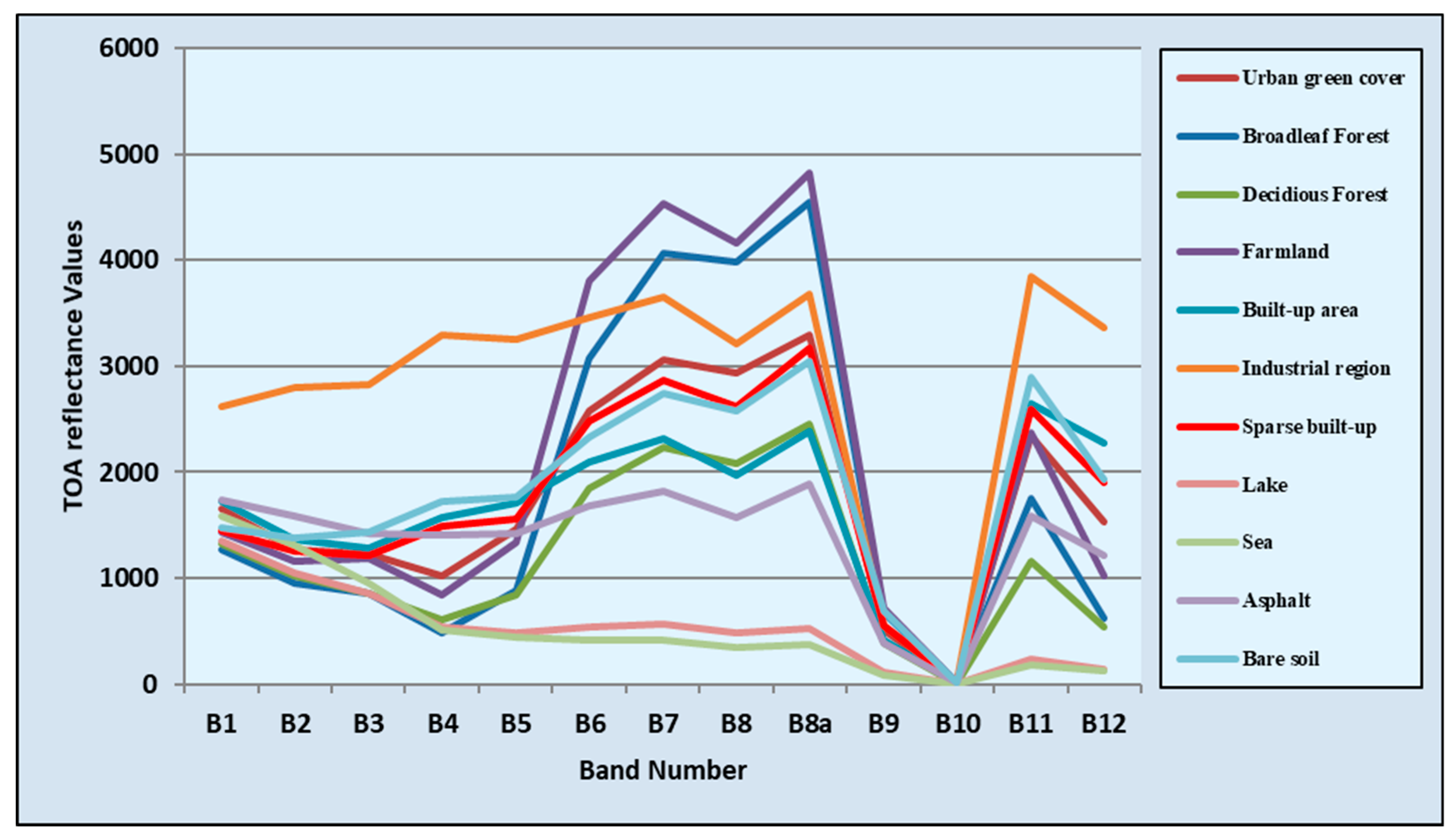
In the next step, spectral profiles of different land object types, including broadleaf forest, deciduous forest, farmland, urban green cover, built-up, industrial region, sparse built-up region, seawater, lake water, asphalt, and bare land, were extracted to examine and compare the separation capacity of the Sentinel-2A image bands (Figure 2). During the classification process, samples from broadleaf and deciduous forest were assigned to the forest class, samples from urban green cover and farmland were assigned to the vegetation class, and samples from lake and sea were assigned to the water class, to obtain the seven land cover types used in this research.

As Figure 2 illustrates, bare land had a similar reflectance to built-up areas and it was difficult to identify these two categories using a single index. It was simple to determine water bodies from other land cover types, due to their unique spectral signature. The gradual decrease of reflectance from band 1 to band 12 was specific to water bodies. A significant reflectance increment in the red-edge bands (B5, B6, B7) and NIR bands (B8, B8a), compared with the red band (B4) was specific to vegetation cover and could be utilized to detect vegetated regions. Additionally, the reflectance curve analyses proved that B1, B9, and B10 (60 m native resolution) could not be used to separate the land cover classes. These observations could be explained by the characteristics of these bands. B1 (coastal aerosol), strongly influenced by the atmosphere and by B9 and B10, which were water vapour and cirrus, did not provide spectral information about the Earth’s surface [54]. Thus, these bands were removed from the data and further analyses was performed with the remaining 10 bands. The spectral evaluation showed that the main challenge was to separate the bare land and the built-up areas, which was the principal objective of this research. Therefore, it aimed to evaluate the existing built-up indices as a first step and proposed an alternative index for those cases that had a lower efficiency. The next step was to suggest a strategy to improve the overall LCU classification results, using the multi-index data composed of three spectral indices, which were sensitive to built-up area/bare land, vegetation cover, and waterbodies, respectively.

4.2. Generating Multi-Index Images

The suitable index combination selection was performed by an experimental analysis of the various combinations of indices as components of the multi-index dataset. For the built-up component, the existing built-up indices and NDTI were examined. Detailed evaluations of the existing built-up indices and the NDTI are provided in Section 4.3 and Section 4.4.

For the vegetation cover component, the red-edge-based normalized difference vegetation index (NDVIre), and two well-known vegetation indices, the soil-adjusted vegetation index (SAVI) [34], and NDVI [55], were examined. Hansen et al. [56], had first evaluated the NDVIre by analyzing hyperspectral reflectance data. Delgado et al. [57] and Frampton et al. [58] had first tested its applicability on the designed Sentinel-2 wavelength portions, before the launch of satellite mission, using data from several ESA field campaigns over agricultural sites. The results of both studies demonstrated that the application of this index to the Sentinel-2 red B4 (665 nm) and the new red-edge B5 (705 nm) bands, provided high correlations during estimation of the leaf area index and the chlorophyll content. Pu et al. [59] and Zhu et al. [60] introduced the operational use of this index for the Worldview-2 satellite imagery. To the best of our knowledge, this research is a novel evaluation of the NDVIre on operational Sentinel-2A imagery.

Lastly, for the water body component, the normalized difference water index (NDWI) and modified normalized difference water index (MNDWI) were examined [61,62].

Table 1. Spectral indices used in this research categorized according to three main LCU classes.

Built-up Areas	Vegetation Cover	Water Bodies
Built-up indices (Table 2)	NDVIre	MNDWI
NDTI	NDVI	NDWI
	SAVI

summarizes the spectral indices that were used to produce the multi-index images, according to the three main LCU categories.

The formulas related to the above spectral indices were:

$$\mathrm{NDTI}=\left(\left(\mathrm{SWIR}1-\mathrm{SWIR}2\right)\right)/\left(\left(\mathrm{SWIR}1+\mathrm{SWIR}2\right)\right)$$

(1)

$$\mathrm{NDVIre}=\left(\left(\mathrm{RedEdge}1-\mathrm{Red}\right)\right)/\left(\left(\mathrm{RedEdge}1+\mathrm{Red}\right)\right)$$

(2)

$$\mathrm{NDVI}=\left(\left(\mathrm{NIR}-\mathrm{Red}\right)\right)/\left(\left(\mathrm{NIR}+\mathrm{Red}\right)\right)$$

(3)

$$\mathrm{SAVI}=\left(\left(\mathrm{NIR}-\mathrm{Red}\right)\right)/\left(\left(\mathrm{NIR}+\mathrm{Red}+0.5\right)\right)\times 1.5$$

(4)

$$\mathrm{NDWI}=\left(\left(\mathrm{Green}-\mathrm{NIR}\right)\right)/\left(\left(\mathrm{Green}+\mathrm{NIR}\right)\right)$$

(5)

$$\mathrm{MNDWI}=\left(\left(\mathrm{Green}-\mathrm{SWIR}1\right)\right)/\left(\left(\mathrm{Green}+\mathrm{SWIR}1\right)\right)$$

(6)

4.3. Experimental Comparison of the Existing Built-Up Indices

The main concern for LCU classification in urban areas is the separation of bare land and built-up areas, due to their similar spectral characteristics. Extracting the bare land is a challenging task, due to the complexity of soil components and soil spectra. As Ben-Dor et al. [63] stated, the chemical constituent directly influences the spectral signature of bare lands, which can be strong or weak. In addition, many of these spectral signatures overlap one another, which makes it difficult to determine soil cover. Accordingly, the spectral characteristics of soil cover, with different components and water content, can vary across different environments and seasons, which makes it difficult to differentiate bare land.

Several indices using different combinations of spectral bands were proposed for mapping built-up areas.

Table 2. Existing built-up indices.

Index Name	Index ID	Bands Used	Formula	Application	Reference
Normalized difference built-up index	NDBI	SWIR and NIR	$\frac{\mathrm{SWIR}-\mathrm{NIR}}{\mathrm{SWIR}+\mathrm{NIR}}$	Automatically mapping urban areas	Zha et al. [37]
Built-up index	BUI	SWIR, NIR and Red	$\mathrm{NDBI}-\mathrm{NDVI}$	Mapping urban built-up areas	He et al. [31]
Built-up area extraction index	BAEI	Red, Green and SWIR	$\frac{\mathrm{Red}+\mathrm{L}}{\mathrm{Green}+\mathrm{SWIR}}$ L = 0.3	Extraction of built-up area	Bouzekri et al. [64]
New built-up index	NBI	Red, NIR and SWIR	$\frac{\mathrm{SWIR}\times \mathrm{Red}}{\mathrm{NIR}}$	Automating the process of mapping residential areas	Jieli et al. [65]
Vegetation index built-up index	VIBI	Red, NIR and SWIR	$\frac{\mathrm{NDVI}}{\mathrm{NDVI}+\mathrm{NDBI}}$	Segmenting urban areas	Stathakis et al. [66]
Index-based built-up index	IBI	Red, Green, NIR and SWIR	$\frac{\mathrm{NDBI}-\left(\mathrm{SAVI}+\mathrm{MNDWI}\right)/2}{\mathrm{NDBI}+\left(\mathrm{SAVI}+\mathrm{MNDWI}\right)/2}$	Enhancing the built-up land feature while effectively suppressing background noise	Xu. [67]
Urban index	UI	NIR and SWIR	$\left(\frac{\mathrm{SWIR}-\mathrm{NIR}}{\mathrm{SWIR}-\mathrm{NIR}}+1.0\right)\times 100$	Evaluating urbanization	Kawamura et al. [68]
Bare soil index	BSI	Red, Blue, NIR and SWIR	$\frac{\left(\mathrm{SWIR}+\mathrm{R}\right)-\left(\mathrm{NIR}+\mathrm{B}\right)}{\left(\mathrm{SWIR}+\mathrm{R}\right)+\left(\mathrm{NIR}+\mathrm{B}\right)}$	Enhancing bare soil areas, fallow lands	Roy et al. [69]

provides a summary of previously introduced built-up indices used in this research [31,37,64,65,66,67,68,69].

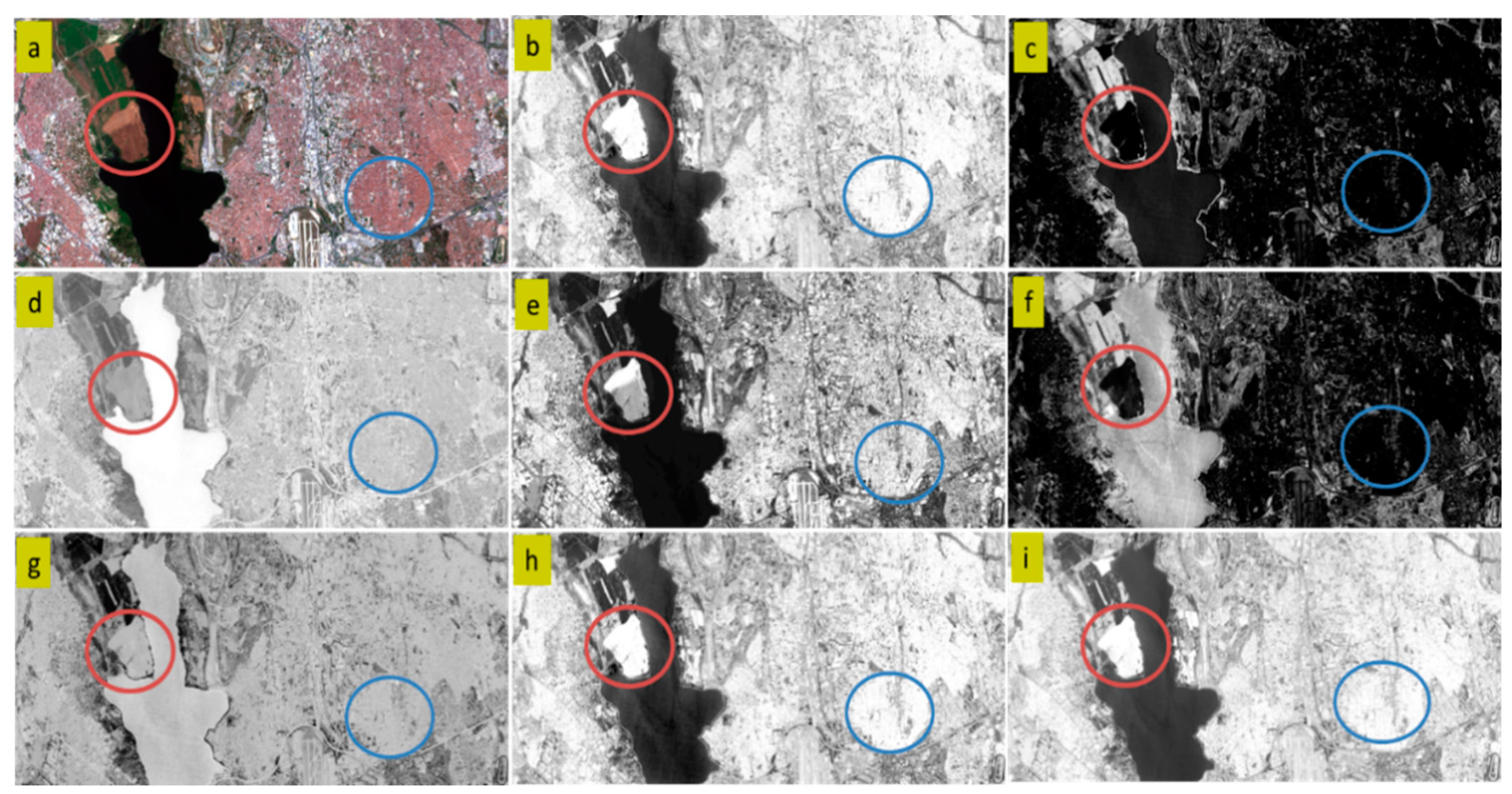
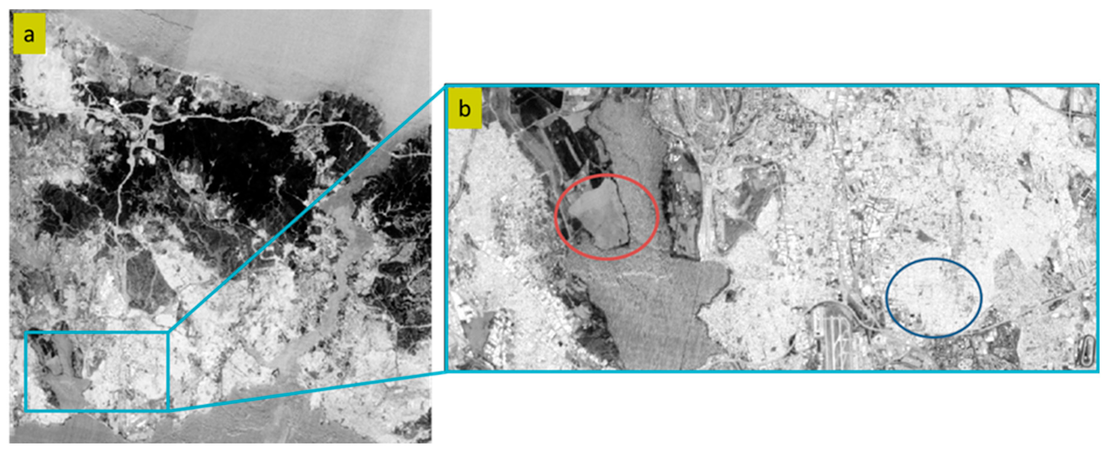
As illustrated in Figure 3, the built-up indices listed in Table 2 can highlight the urban areas and separate them from the water bodies and vegetation cover. However, detailed inspection revealed that these indices could not separate the bare land from the built-up areas, in most cases. The region marked by a blue circle corresponds to the built-up area covered by buildings and impervious surfaces and the region marked by a red circle shows an empty farmland covered by bare soil. There was no major contrast between these two regions in the index images, indicating a low separability between the two land cover classes. The NBI image provided a slight contrast difference between the urban area and the soil cover, compared to the other indices, but not enough for an accurate separation (Figure 3e). The BSI, which is mostly used for determining bare land, in the literature, was not successful in separating the bare land from the built-up areas. Visual interpretation results of the BSI image showed that the urban area and the bare land were highly mixed. The urban areas, composed of buildings with brown roofs, showed a similar spectral response to that of bare land, which made them possible candidates for getting mixed-up (Figure 3i). The initial visual analysis indicated the necessity for an index that could highlight the built-up area and separate it from the soil cover.

4.4. Normalized Difference Tillage Index (NDTI)

To propose an index that can highlight built-up areas and separate them from bare land, the spectral profiles of these two land features were analyzed at several sample locations. It showed that the reflectance difference between the SWIR bands (bands 11 and 12) was higher for the pixels selected from the bare land than for the pixels selected from the built-up areas. This indicated the possible efficiency of these two SWIR bands for differentiating built-up area from bare land. The applicability of the NDTI on SWIR bands of the Sentinel-2A images for built-up area and bare land extraction was investigated. This index was first proposed by van Deventer et al. [70] for soil practices, tillage management, and crop residue mapping, and was successfully applied by Daughtry et al. [71] and Eskandari et al. [72] for agricultural practices and soil management. To our knowledge, this is the first time that the NDTI has been used as a component to discriminate and separate built-up areas and bare land.

The NDTI data provided in Figure 4 and the existing built-up indices provided in Figure 3 show that the NDTI can highlight the urban areas and it increases the contrast between the bare land (red circle) and built-up area (blue circle). This visual inspection indicates the possible efficiency of the NDTI, compared to the existing built-up indices.

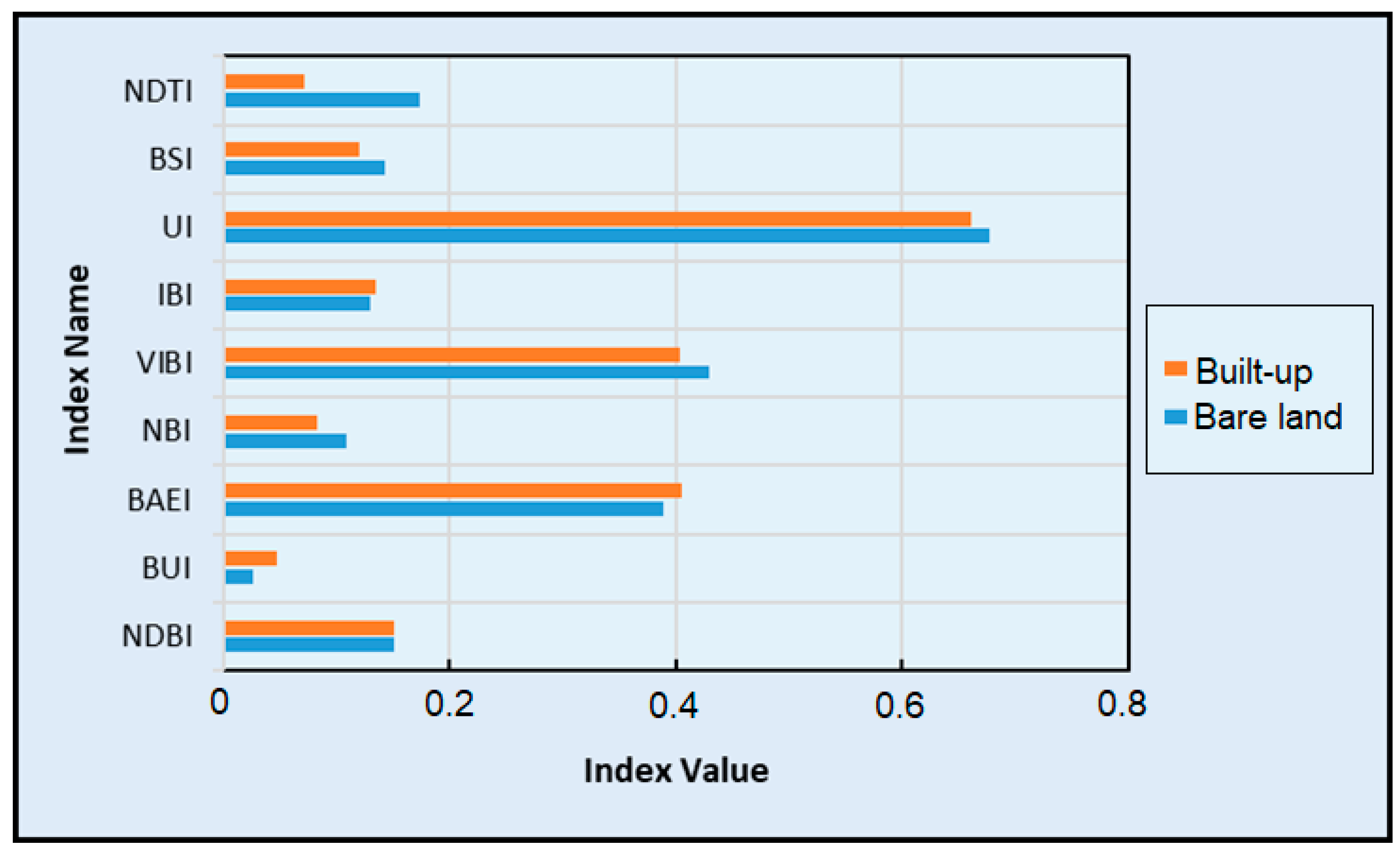
As a second analysis, 80 random points (40 for each class) were selected and the mean index values were calculated to statistically evaluate the capability of the NDTI in separating the bare land from the built-up areas. As illustrated in Figure 5, the NDTI provides distinctive values for bare land and built-up area classes, whereas the existing built-up indices provide similar values.

While the NDTI increases the contrast between bare land and built-up areas, it decreases the contrast between water bodies and other land covers (Figure 4). This drawback is overcome by the multi-index approach proposed in this research.

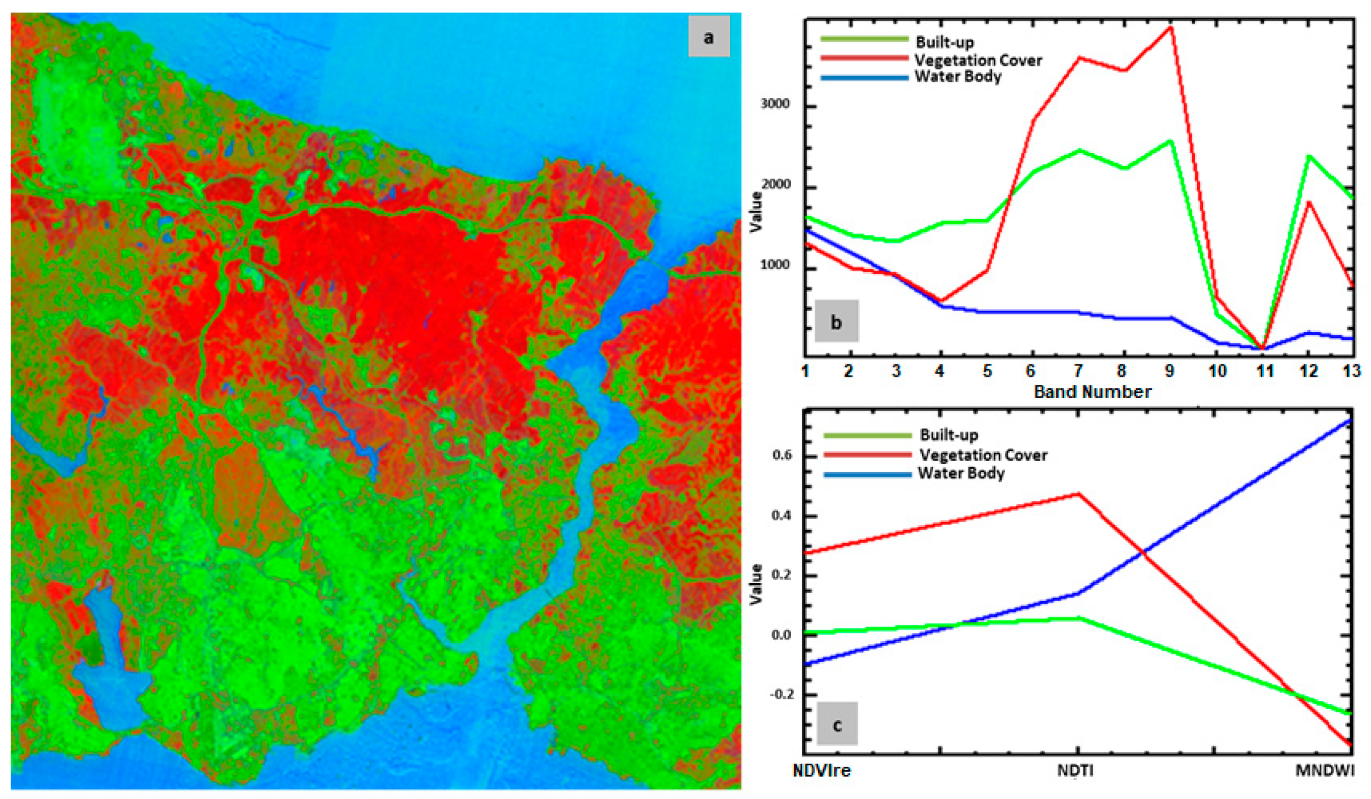
Figure 6a shows an RGB composite multi-index image produced from the NDTI, the NDVIre, and the MNDWI. This multi-index image provides a good discrimination between the three major LC categories—vegetation cover in red, water bodies in blue, and the built-up areas in green. The spectral signature analysis shows that the multi-index dataset represents a more linear and simplified response for the main LC categories than the original image bands, which indicates a better separation capability (Figure 6b,c).

4.5. Classification and Accuracy Assessment

To examine the capability of the multi-index approach in extracting the built-up area and determining the other LCU classes, the SVM classification method with radial basis function (RBF) kernel was applied on the multi-index images. The SVM was initially developed as a binary classifier, thus, a pairwise classification approach was implemented for multiclass classification requirements, by creating a binary classifier for each possible pair of classes [73]. The classification process was performed using the ENVI software, which requires a set of parameter definitions. The gamma is the most critical parameter and was the only parameter changed in this research (determined by division of 1 by the number of data layers). The penalty parameter reduces misclassification in the training step when set to 100. The classification probability threshold should be set to zero to guarantee that each pixel is assigned to a class. A pyramid level of zero allows for the classification to be performed directly on the original image pixels, instead of a first-pass classification on low-resolution pyramid layers [74].

The built-up index data listed in Table 2 and the NDTI were separately layer-stacked with vegetation and water index data and were classified using the same training samples, defined by region of interest (ROI). In addition, the ten-band Sentinel-2A image was classified and compared with the multi-index image classification results to analyze and illustrate the improvements in the classification accuracy, using the index images. Lastly, the NDTI-based multi-index dataset was layer-stacked with the ten-band original image and this thirteen-band combination was also classified for further comparison.

To evaluate the accuracy of the classification results, the overall accuracies with the user’s, the producer’s, and the overall accuracy metrics and Kappa statics were derived from the confusion matrix [75]. The accuracy assessment of the classification results was performed with stratified random points, and the original Sentinel-2A image and Google Earth© imagery as the reference data. A random point distribution was designed, according to the heterogeneity potential and areal coverage of the classes. The training sample distribution and number of points used in the accuracy assessment are provided for each class and region in

Table 3. Training sample and accuracy assessment point distribution for the study regions.

	Training Sample						Number of Accuracy Assessment Points
Class Name/ Region	Istanbul		Ankara		Konya		Istanbul	Ankara	Konya
	Poly.	Pix.	Poly.	Pix.	Poly.	Pix.	Point	Point	Point
Bare Land	215	1874	67	12198	72	42070	250	185	250
Asphalt	47	473	25	360	19	1033	60	40	50
Water	18	1587	2	4543	1	636	40	15	10
Industry	26	198	4	72	12	731	70	30	50
Built-up	333	1326	295	629	84	1373	250	185	250
Forest	173	5184	8	565	6	85	70	25	20
Veg. Cover	81	4458	4	118	17	2206	70	45	25
Total	893	15100	405	18485	211	48134	810	525	655

.

5. Results and Discussion

5.1. Results for the Main Study Region

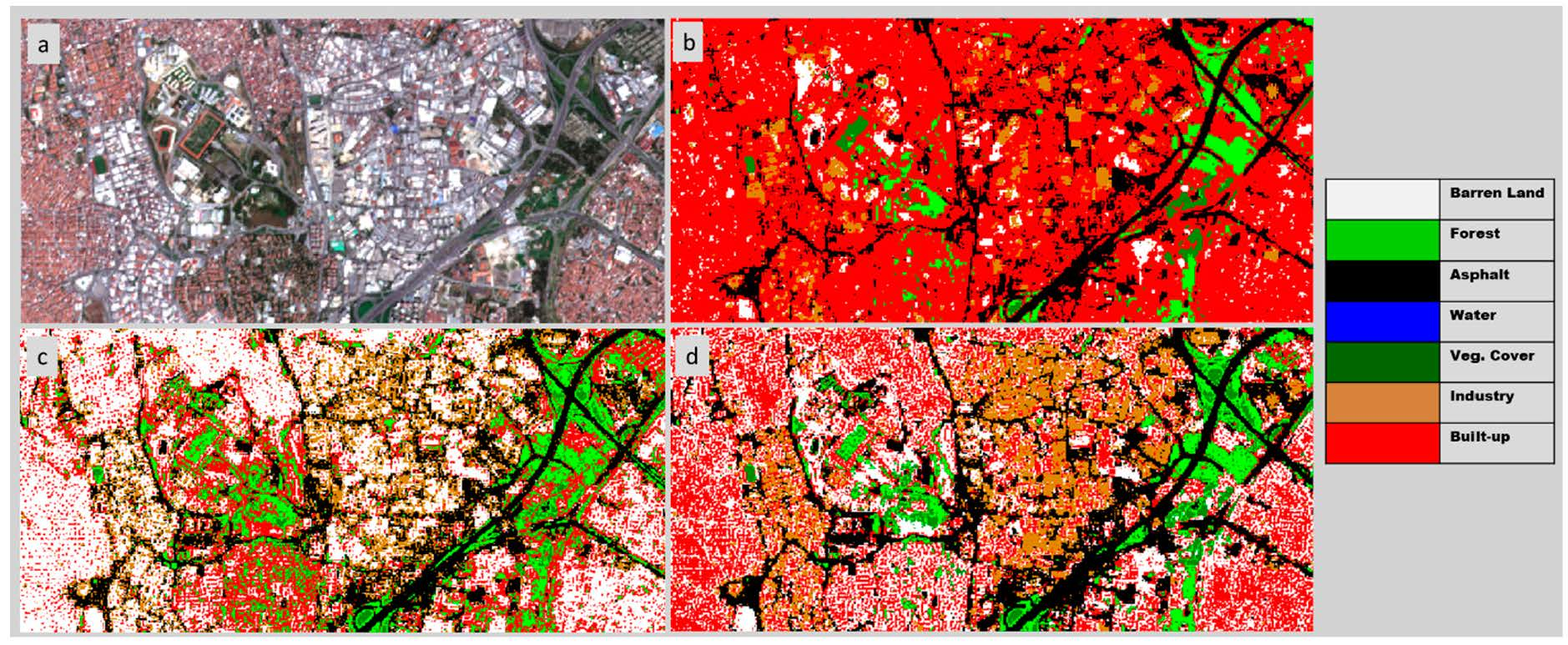
The classification results and accuracy assessment metrics showed that the NDTI, in combination with NDVIre and the MNDWI, provided the highest accuracy, in comparison to other combinations including the existing built-up indices and the original image classification (

Table 4. Classification accuracies of the different approaches for the Istanbul region.

	(Sentinel-2A Image (10 Bands))		(NDBI+NDVIre+MNDWI)		(NDTI+NDVIre+MNDWI)
Land Cover Class	Producer’s Accuracy (%)	User’s Accuracy (%)	Producer’s Accuracy (%)	User’s Accuracy (%)	Producer’s Accuracy (%)	User’s Accuracy (%)
Bare land	90.78	55.49	53.32	61.13	92.90	92.11
Asphalt	93.75	100	72.50	96.67	85.71	100.00
Water	100	97.50	100.00	97.50	100.00	97.50
Industry	96.77	85.71	92.68	54.29	98.28	81.43
Built-Up	62.77	95.20	40.79	34.32	93.28	92.25
Forest	62.89	100	81.90	86.00	94.23	98.00
Veg. Cover	78.57	45.71	81.82	77.14	93.33	100.00

and

Table 5. Comparison of the overall accuracy and Kappa statistics for the Istanbul region.

Data Type	Overall Accuracy	Kappa
Sentinel-2A image (10 Bands)	0.75	0.67
Multi-index (NDBI+NDVIre+MNDWI)	0.60	0.47
Multi-index (NDTI+NDVIre+MNDWI)	0.93	0.91

). Visual analysis of the resulting images in Figure 7 shows that the NDTI solves the mixing problem of the built-up and the bare land, which is obvious in other built-up indices. In addition, the problems related to overestimation of built-up regions and underestimation of bare land improved significantly, using this combination. The second highest accuracy was achieved with the combination of NDBI, NDVIre, and MNDWI, for all multi-index combinations. This result was in accordance with NDBI’s reported performance in built-up area detection [76]. However, this combination provided lower overall accuracies and a low rate of bare land detection, compared to the NDTI-based combination and original image classification results. These results strengthened the findings regarding the built-up indices described in Section 4.3.

According to the per-class accuracy results presented in the Table 4, the multi-index image of the NDBI, the NDVIre, and the MNDWI, provided lower accuracies than the ten-band original Sentinel-2A image for most land cover classes, except for improvements in the vegetation cover class. This improvement can be explained by the use of the NDVIre index, which includes the red-edge band of the Sentinel-2A, for vegetation monitoring. However, this combination could not provide a reliable separation between the built-up area and the bare land. The multi-index image of the NDTI, the NDVIre, and the MNDWI provided better accuracies for most of the land cover classes, especially the built-up and the bare land classes. Similarly, the red-edge band included in the NDVIre provided superior information about vegetation cover class. The overall accuracy and kappa metric presented in Table 5 indicated that the NDTI-based combination improved the accuracy metrics with consistent ranges for each individual LCU class, compared to the classified Sentinel-2A image and classified multi-index image of the NDBI, the NDVIre, and the MNDWI.

As an additional experiment, three indices, including the NDTI, the NDVIre, and the MNDWI were stacked with the original Sentinel-2A ten bands and the resultant image with thirteen layers (ten original bands and three index images) was classified using the same ROIs; however, the classification result did not show a satisfying performance. Notably, the NDTI-based multi-index approach could not completely solve the problem of mixed pixels of bare land and built-up area, but showed an evident improvement, compared to other built-up indices and original image classifications.

The sub regions from the classification results of Istanbul are provided in the following figures (Figure 8, Figure 9 and Figure 10) to demonstrate the improvements of the proposed NDTI-based method, over other classification results. In addition, the accuracy assessment results of these sub regions are given in

Table A1. Classification accuracies of the different approaches for Figure 8.

	(Sentinel-2A Image (10 Bands))		(NDBI+NDVIre+MNDWI)		(NDTI+NDVIre+MNDWI)
Land Cover Class	Producer’s Accuracy (%)	User’s Accuracy (%)	Producer’s Accuracy (%)	User’s Accuracy (%)	Producer’s Accuracy (%)	User’s Accuracy (%)
Bare land	45.00	81.82	75.00	23.07	97.50	95.12
Asphalt	92.00	100.00	88.00	78.57	100.00	100.00
Water	100.00	100.00	85.00	94.44	100.00	100.00
Industry	60.00	100.00	70.00	77.77	100.00	100.00
Built-Up	88.00	64.70	74.00	50.00	96.00	97.95
Forest	96.00	42.10	72.00	64.28	100.00	100.00
Veg. Cover	22.85	100.00	80.00	80.00	100.00	100.00

,

Table A2. Comparison of the overall accuracy and the Kappa statistics for Figure 8.

Data Type	Overall Accuracy	Kappa
Sentinel-2A image (10 Bands)	0.70	0.64
Multi-index (NDBI+NDVIre+MNDWI)	0.64	0.56
Multi-index (NDTI+NDVIre+MNDWI)	0.98	0.98

,

Table A3. Classification accuracies of the different approaches for Figure 9.

	(Sentinel-2A Image (10 Bands))		(NDBI+NDVIre+MNDWI)		(NDTI+NDVIre+MNDWI)
Land Cover Class	Producer’s Accuracy (%)	User’s Accuracy (%)	Producer’s Accuracy (%)	Land Cover Class	Producer’s Accuracy (%)	User’s Accuracy (%)
Bare land	23.07	93.75	36.92	36.92	89.23	90.62
Asphalt	100.00	95.65	90.90	76.93	100.00	91.66
Industry	56.00	87.50	60.00	78.94	92.00	100.00
Built-Up	100.00	44.45	22.91	21.56	89.58	87.75
Forest	72.00	58.06	87.40	61.76	100.00	100.00
Veg. Cover	60.00	57.14	66.67	100.00	96.66	96.66

,

Table A4. Comparison of the overall accuracy and Kappa statistics for Figure 9.

Data Type	Overall Accuracy	Kappa
Sentinel-2A image (10 Bands)	0.62	0.54
Multi-index (NDBI+NDVIre+MNDWI)	0.51	0.39
Multi-index (NDTI+NDVIre+MNDWI)	0.93	0.91

,

Table A5. Classification accuracies of different approaches for Figure 10.

	(Sentinel-2A Image (10 Bands))		(NDBI+NDVIre+MNDWI)		(NDTI+NDVIre+MNDWI)
Land Cover Class	Producer’s Accuracy (%)	User’s Accuracy (%)	Producer’s Accuracy (%)	Land Cover Class	Producer’s Accuracy (%)	User’s Accuracy (%)
Bare land	44.44	83.33	26.66	66.66	91.11	91.11
Asphalt	66.66	83.33	70.00	80.76	70.00	91.30
Water	100.00	100.00	80.00	100.00	95.00	100.00
Industry	53.84	100.00	61.53	100.00	76.92	100.00
Built-Up	66.66	15.00	55.55	9.61	88.88	82.10
Forest	96.00	42.85	60.00	55.55	88.00	84.61
Veg. Cover	62.50	66.66	75.00	88.88	90.62	90.62

and

Table A6. Comparison of the overall accuracy and Kappa statistics for Figure 10.

Data Type	Overall Accuracy	Kappa
Sentinel-2A image (10 Bands)	0.59	0.50
Multi-index (NDBI+NDVIre+MNDWI)	0.58	0.51
Multi-index (NDTI+NDVIre+MNDWI)	0.86	0.83

. The accuracy metrics show the ten-band original image classification and NDBI-based multi-index set classification provided similar accuracies, whereas the NDTI-based multi-index set outperformed them with a 30% overall accuracy improvement and better consistency of the producer’s and the user’s accuracy. These results supported the accuracy assessment results of the whole study region.

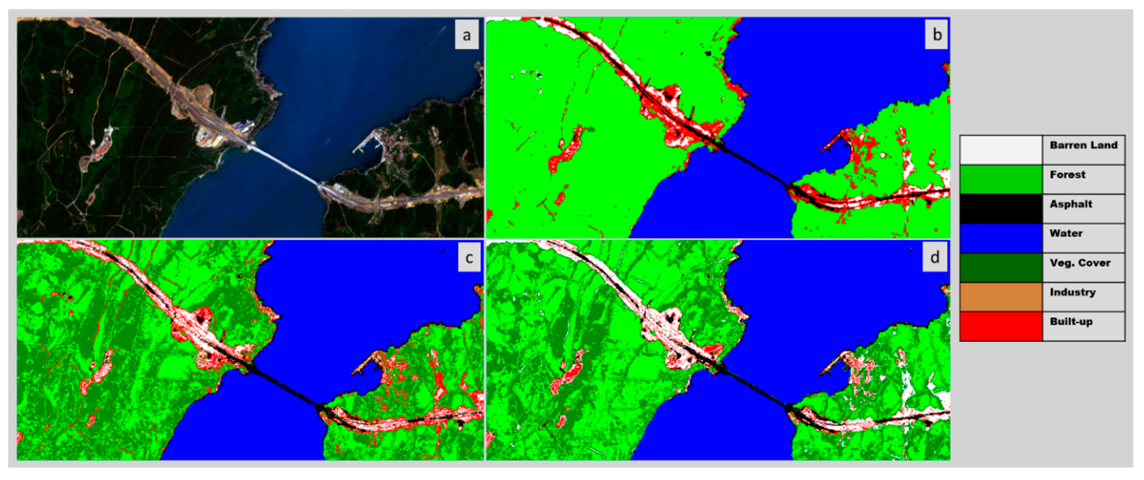
Figure 8 represents regions covered by water, asphalt road, bare land, vegetation covers, and built-up area land cover classes. All classified images accurately classified water bodies and asphalt road, but there was a misclassification of the bare lands as built-up regions in the multi-index images, using the NDBI (Figure 8c) and a misclassification issue and overestimation of the built-up area in the classified Sentinel-2A image (Figure 8b). The multi-index image of the NDTI, the NDVIre, and the MNDWI provided better results than the other two (Figure 8d). The NDTI-based image classification determined the built-up areas, more accurately, and separated the bare land near roads, which were classified as built-up areas in the classified Sentinel-2A image (Figure 8b). The multi-index combinations, including the NDVIre, determined vegetation cover better and improved the separation of different vegetation types in the study area. Different vegetation types can be recognized more obviously in both multi-index images (Figure 8c,d) than in the classified Sentinel-2A image (Figure 8b).

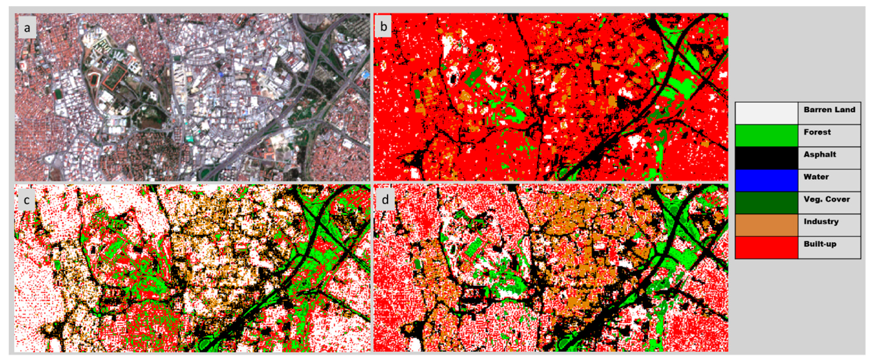
In Figure 9, more complicated and heterogeneous parts of Istanbul were investigated. The area is covered with dense residential and industrial built-up patches and includes highways and urban green areas. According to visual inspection, the original ten-band image classification suffered from overestimation of residential areas and misclassification of industrial areas and bare land (Figure 9b). Additionally, the NDBI-based multi-index image could not separate the industrial areas from residential areas and there was a misclassification problem of the residential areas, due to the overestimation of bare land. These problems were also observed in other built-up, index-based combinations (Figure 9c). The NDTI, in combination with the NDVI and the MNDWI determined the industrial regions more precisely. In such a heterogeneous region, a multi-index image of NDTI, NDVIre, and MNDWI provided superior information about all land cover classes, compared to the other classification results (Figure 9d).

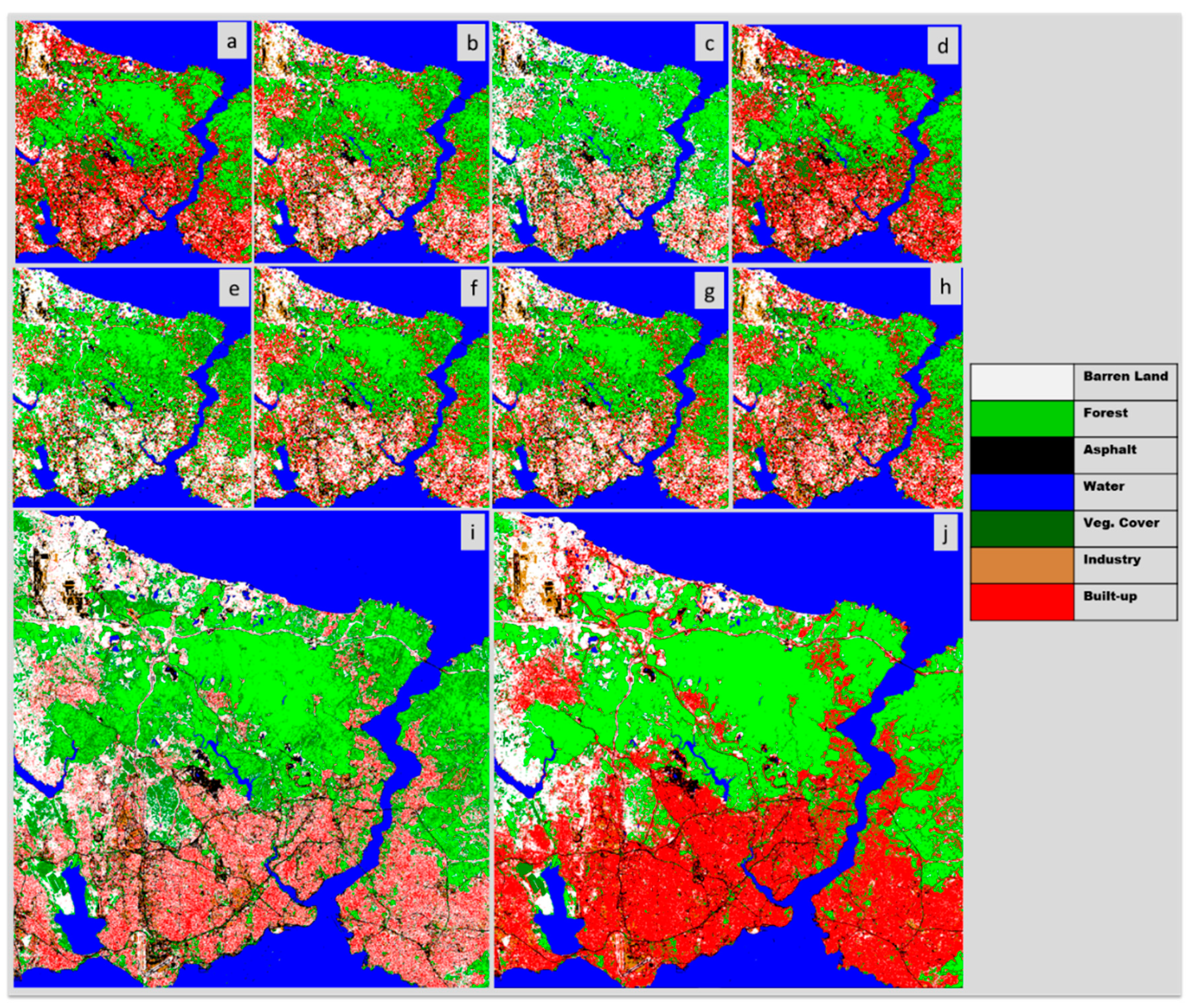
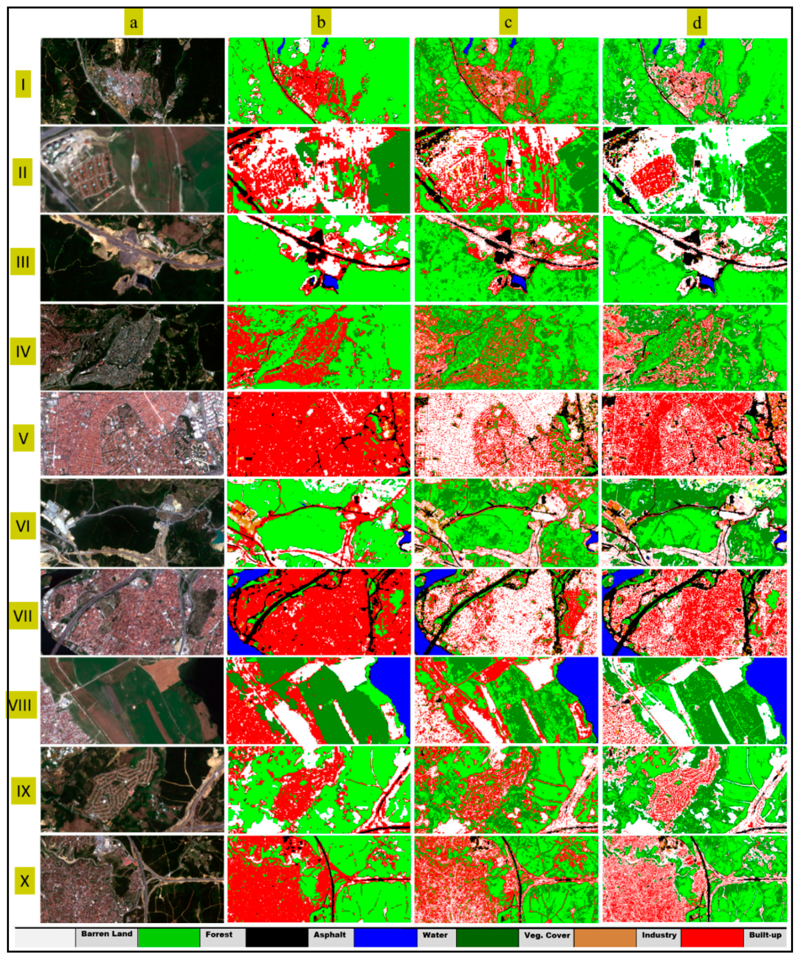
Generally, the multi-index image of the NDTI, NDVIre, and the MNDWI successfully separated bare land from the built-up areas, while categorizing other land cover classes, such as vegetation cover and water body precisely (Figure 10d). Classification of the NDTI-based multi-index set provided a superior understanding of the built-up area patterns and building footprints, especially for the organized types of residential construction (Figure 10(II,IV,IX)) and avoided an overestimation of the built-up areas in the classified Sentinel-2A image (10 bands) (Figure 10b). The other multi-index image generated using the NDBI, the NDVIre, and the MNDWI, using the NDBI as the nominee of the existing built-up indices had an excessive misclassification issue. It classified bare land cover as the built-up class and vice versa (Figure 10c). Farmlands with no vegetation cover and low water content and especially those that were compacted because of the field operations, heavy equipment, and tillage implements were mostly misclassified as built-up regions with the NDBI-based set. This misclassification problem was mostly overcome using the proposed NDTI-based multi-index image (Figure 10 (VIII)). Bare land cover near asphalt roads, which also contained a lower water content, were among the land cover classes that were highly misclassified as built-up areas, and this problem was significantly improved by using the NDTI-based multi-index image (Figure 10(III,VI,X,IX)). Although, the classification results of the NDTI-based multi-index image underestimated the density of the built-up area in some dense built-up regions, the proposed multi-index image classification method provided reliable information about both bare land and built-up classes, while accurately categorizing water and vegetation land cover classes.

5.2. Validation on Independent Test Regions

The efficiency and applicability of the proposed approach was tested in two metropolitan cities of Turkey, Ankara, and Konya. These regions were good candidates for evaluating the performance of the multi-index method because they include residential and industrial areas surrounded by extensive bare land, which suited the main objective of this research. Additionally, the image acquisition dates represented different seasonal conditions. The SVM classification was performed on these regions for the three datasets, which were the original ten-band Sentinel-2A image, the NDBI, NDVIre, MNDWI dataset, and the NDTI, NDVIre, MNDWI dataset. The training sample distribution and the number accuracy assessment points are presented in Table 3.

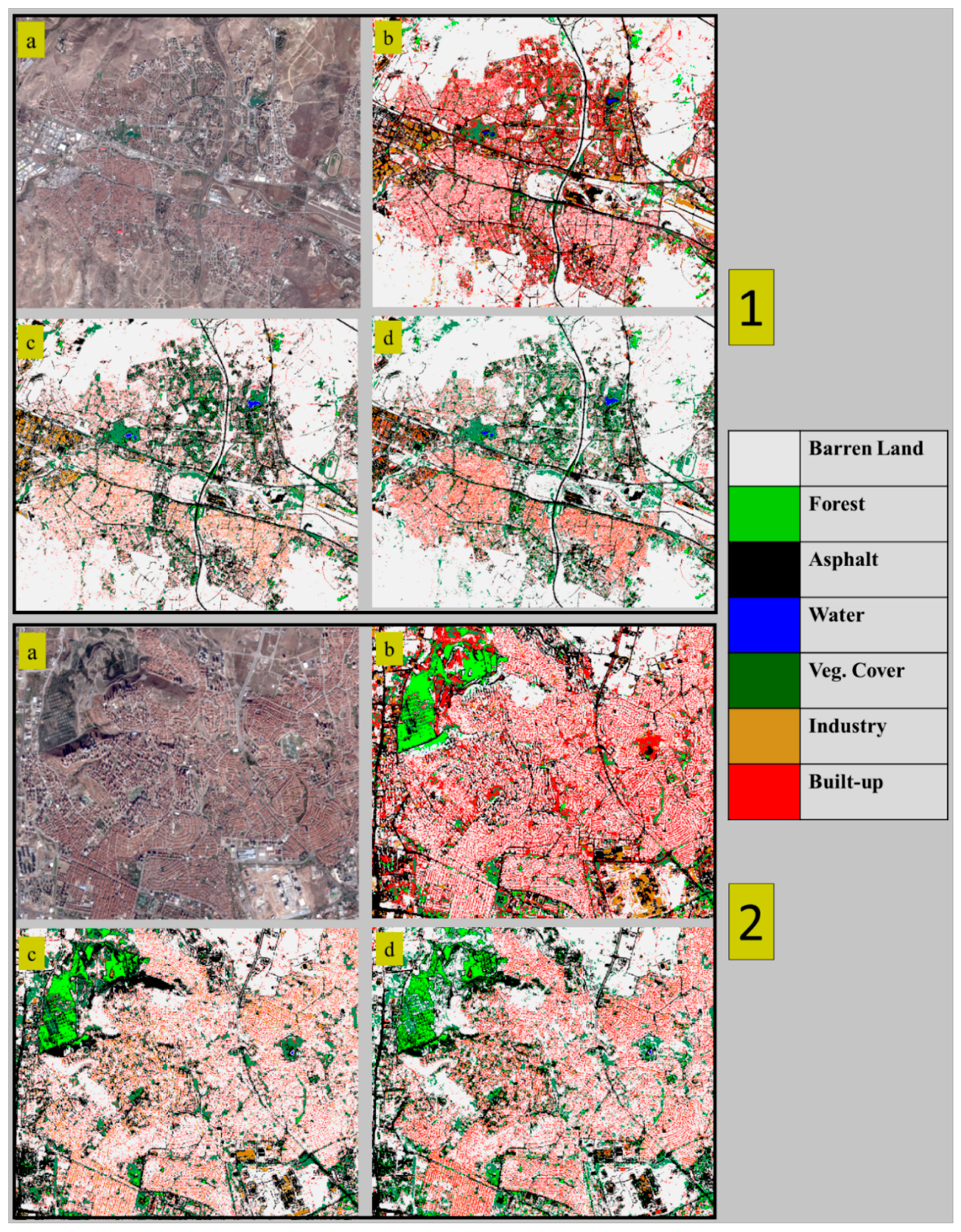
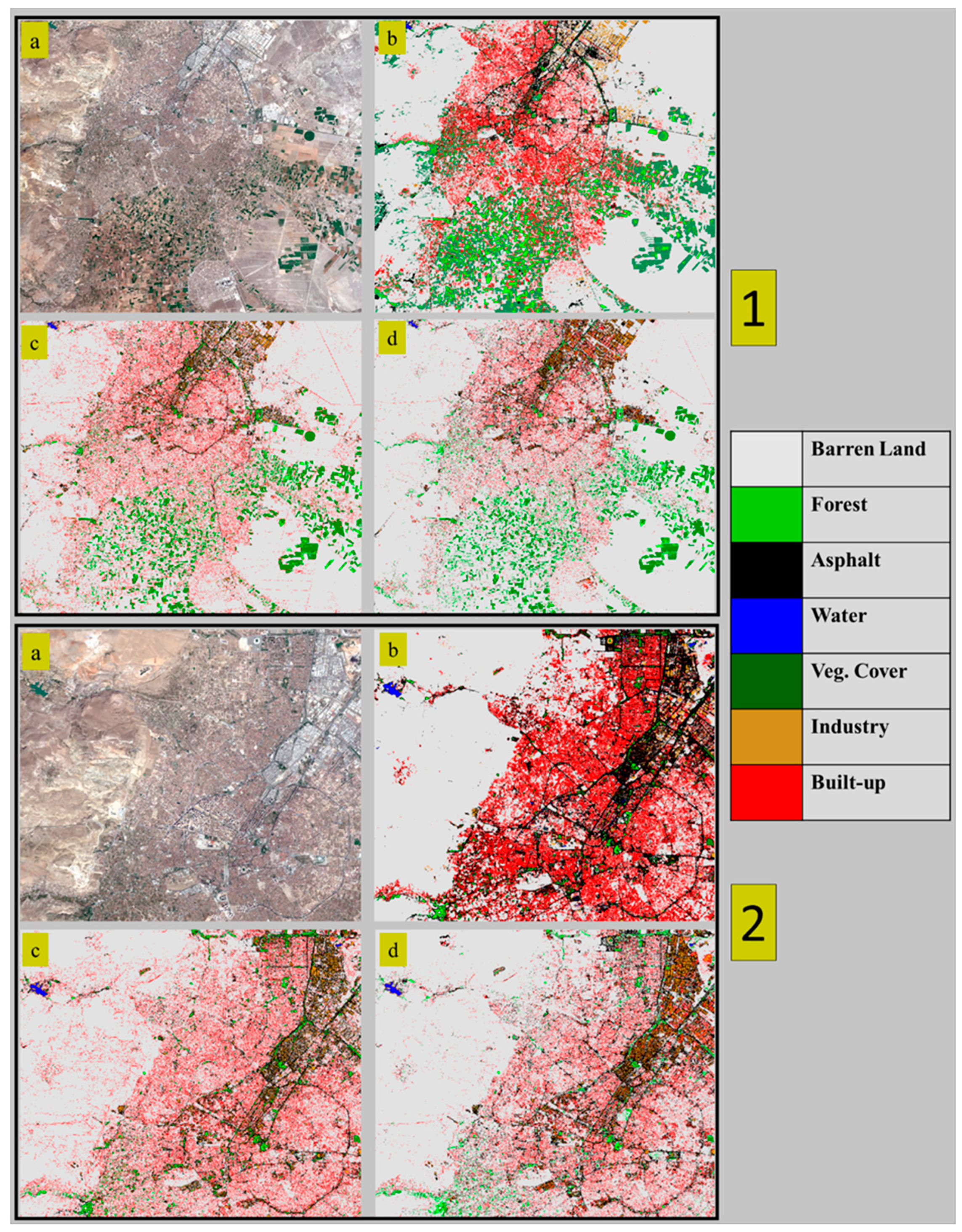
The classification results of the Ankara region are presented in Figure 11 and the accuracy assessment values are provided in

Table 6. Classification accuracies of the different approaches for the Ankara region.

	(Sentinel-2A Image (10 Bands))		(NDBI+NDVIre+MNDWI)		(NDTI+NDVIre+MNDWI)
Land Cover Class	Producer’s Accuracy (%)	User’s Accuracy (%)	Producer’s Accuracy (%)	User’s Accuracy (%)	Producer’s Accuracy (%)	User’s Accuracy (%)
Bare land	59.52	22.73	43.18	34.55	89.77	90.80
Asphalt	97.50	66.10	92.50	84.09	100.00	97.56
Water	100.00	100.00	100.00	100.00	100.00	100.00
Industry	26.67	53.33	70.00	100.00	83.33	100.00
Built-Up	84.34	43.48	20.48	48.57	92.77	92.77
Forest	94.44	65.39	88.89	72.73	100.00	81.82
Veg. Cover	36.36	100.00	93.18	57.75	97.72	95.56

and

Table 7. Comparison of the overall accuracy and Kappa statistics for the Ankara region.

Data Type	Overall Accuracy	Kappa
Sentinel-2A image (10 Bands)	0.51	0.42
Multi-index (NDBI+NDVIre+MNDWI)	0.58	0.48
Multi-index (NDTI+NDVIre+MNDWI)	0.92	0.90

. The results showed that the accuracy improvement using the NDTI-based multi-index image was evident. This combination provided higher accuracies for bare land, industry, and built-up classes, indicating a better separation among them. Additionally, the consistency between the producer’s and the user’s accuracy was higher than that of the other datasets. The overall accuracy was improved by, approximately, 30–40%. The two sub-regions presented in Figure 11 shows that the classification result of the ten–band multispectral image (Regions 1b and 2b) was dominated by the built-up and the industrial lands, and it misclassified the bare land surrounding them, especially in low-density urban areas. There were incorrectly classified regions near the green areas, due to this effect, which occurred in the north-west and east of both sub-regions. The NDBI-based, multi-index set was less affected by this over classification, but it suffered while trying to distinguish between industry and built-up classes and false classification occurred due to labelling an extensive amount of the built-up areas as industrial land (Regions 1c and 2c).

The classification results of the Konya region are presented in Figure 12 and the accuracy assessment values are provided in

Table 8. Classification accuracies of different approaches for the Konya region.

	(Sentinel-2A Image (10 Bands))		(NDBI+NDVIre+MNDWI)		(NDTI+NDVIre+MNDWI)
Land Cover Class	Producer’s Accuracy (%)	User’s Accuracy (%)	Producer’s Accuracy (%)	User’s Accuracy (%)	Produce’s Accuracy (%)	User’s Accuracy (%)
Bare land	21.13	77.77	34.95	40.56	91.05	77.24
Asphalt	96.42	47.36	46.42	37.14	96.42	75.00
Water	100.00	100.00	100.00	100.00	100.00	100.00
Industry	68.18	96.77	61.36	96.42	84.09	100.00
Built-Up	77.77	50.90	53.70	42.02	70.37	89.41
Forest	45.00	69.23	35.00	70.00	95.00	86.36
Veg. Cover	78.26	54.54	82.60	65.51	86.95	95.23

and

Table 9. Comparison of the overall accuracy and Kappa statistics for the Konya region.

Data Type	Overall Accuracy	Kappa
Sentinel-2A image (10 Bands)	0.57	0.45
Multi-index (NDBI+NDVIre+MNDWI)	0.49	0.33
Multi-index (NDTI+NDVIre+MNDWI)	0.84	0.79

. The accuracy improvement and consistency between the producer’s and the user’s accuracy with the NDTI-based dataset was similar to that in the Ankara region, and the other datasets suffered from low accuracies for the bare land, built-up, and the industry classes. The evaluation in Figure 12 shows that the ten-band multispectral imagery classification over-classified built-up lands and could not detect the industrial areas, which could be seen clearly in Region 2b. For the NDBI-based dataset, the bare land in the western part of Regions 1 and 2 were over-classified as built-up land (Regions 1c and 2c). Moreover, there were improvements in the accuracy metrics of the asphalt, forest, and vegetation classes, when applying the proposed method (Regions 1d and 2d).

The analysis of the two independent test regions showed similar characteristics and supported the effectiveness of the NDTI-based multi-index set in different land and seasonal conditions. Notably, the roofs of buildings in industrial areas were made of aluminium-based materials and concrete, whereas the roofs of the other buildings in the built-up areas were made of tiles in the main and in the test regions. The difference in the roof material resulted in different spectral responses and enabled separation in the original spectral bands and the multi-index data for these classes. Thus, the mixing problem was mainly between bare land and the built-up areas and between bare land and industry. Further analysis was required to evaluate the performance of the proposed approach in regions where the industrial and built-up areas were composed of similar roof materials.

The results from the study and the test regions demonstrated that although built-up indices have been shown to highlight built-up areas, their performance was limited in heterogeneous landscapes, where urban areas and bare lands were mixed. A shortwave infrared-based index improved the separation of urban areas and bare lands, as shown in this research work. In addition, the newly added red-edge spectral bands of Sentinel-2A enhanced the vegetation cover detection and mapping.

6. Conclusions

Separating bare land from the impervious surfaces and built-up areas has been the main problem in mapping urbanized areas. In this research work, a novel multi-index approach has been proposed for the LCU classification of Sentinel-2A satellite images, focusing on separating the urban and bare land, in addition to other land cover categories. To improve the classification accuracy and solve the misclassification and overestimation problems, a methodology was developed using spectral indices that categorized the three major land cover classes, water bodies, vegetation cover, and built-up areas. The multi-index images created with different index combinations were classified using the machine-learning-based SVM algorithm. The multi-index classification results were compared with the SVM classification result of the ten-band Sentinel-2A image. The results of this research showed that NDTI in combination with NDVIre and MNDWI improved the separation between the built-up regions and bare land, and significantly improved the misclassification of bare lands as built-up regions. In addition, the NDTI, which was calculated by the difference of the SWIR bands, divided by its sum of them, could be applied to the Landsat 5, 7, and 8 images, as well as the Landsat missions that included the SWIR bands with a similar wavelength range of the Sentinel-2 mission. This applicability enabled a further analysis using combined historic archival Landsat missions and higher spatial and spectral resolution Sentinel-2A images, to detect LCU changes through decades. Although classification of the ten-band Sentinel-2A imagery provided acceptable results related to the built-up area and bare land classes, the multi-index image of the NDTI, the NDVIre, and the MNDWI provided more interpretable and illustratable results for the built-up regions, in terms of shape, intensity, and pattern. The proposed combination also provided satisfactory results and accuracy improvements for the other LCU classes, with 85% or better accuracy in the three study regions, compared to other datasets. These findings indicate the possible effectiveness of the proposed multi-index set as a dimension reduction method in multi-temporal analysis. Further studies are planned to integrate multi-temporal and multi-polarization SAR data, such as Sentinel 1 (to process chain), in order to take advantage of the SAR data in the separation of bare lands and built-up areas.

References

- Yuan, F.; Sawaya, K.E.; Loeffelholz, B.C.; Bauer, M.E. Land cover classification and change analysis of the Twin Cities (Minnesota) Metropolitan Area by multitemporal Landsat remote sensing. Remote Sens. Environ. 2005, 98, 317–328. [Google Scholar] [CrossRef]
- Masek, J.G.; Lindsay, F.E.; Goward, S.N. Dynamics of urban growth in the Washington DC metropolitan area, 1973–1996, from Landsat observations. Int. J. Remote Sens. 2000, 21, 3473–3486. [Google Scholar] [CrossRef]
- Sertel, E.; Robock, A.; Ormeci, C. Impacts of land cover data quality on regional climate simulations. Int. J. Clim. 2010, 30, 1942–1953. [Google Scholar] [CrossRef]
- Mahmood, R.; Pielke, R.A., Sr.; Hubbard, K.G.; Bonan, G.; Lawrence, P.; Baker, B.; McNider, R.; McAlpine, C.; Etter, A.; Gameda, S.; et al. Impacts of land use landcover change on climate and future research priorities. Bull. Am. Meteorol. Soc. 2010, 91, 37–46. [Google Scholar] [CrossRef]
- Mahmood, R.; Pielke, R.A.; Hubbard, K.G.; Niyogi, D.; Dirmeyer, P.A.; McAlpine, C.; Carleton, A.M.; Hale, R.; Gameda, S.; Beltrán-Przekurat, A.; et al. Land cover changes and their biogeophysical effects on climate. Int. J. Climatol. 2014, 34, 929–953. [Google Scholar] [CrossRef]
- Luyssaert, S.; Jammet, M.; Stoy, P.C.; Estel, S.; Pongratz, J.; Ceschia, E.; Churkina, G.; Don, A.; Erb, K.; Ferlicoq, M. Land management and land-cover change have impacts of similar magnitude on surface temperature. Nat. Clim. Chang. 2014, 4, 389–393. [Google Scholar] [CrossRef] [Green Version]
- Li, H.; Walter, M.; Wang, X.; Sodoudi, S. Impact of land cover data on the simulation of urban heat island for Berlin using WRF coupled with bulk approach of Noah-LSM. Theor. Appl. Climatol. 2018, 134, 67–81. [Google Scholar] [CrossRef]
- Aburas, M.M.; Ho, Y.M.; Ramli, M.F.; Ash’aari, Z.H. The simulation and prediction of spatio-temporal urban growth trends using cellular automata models: A review. Int. J. Appl. Earth Obs. Geoinf. 2016, 52, 380–389. [Google Scholar] [CrossRef]
- Sertel, E.; Akay, S.S. High resolution mapping of urban areas using SPOT-5 images and ancillary data. Int. J. Environ. Geoinform. 2015, 2, 63–76. [Google Scholar] [CrossRef] [Green Version]
- Wardell, D.A.; Reenberg, A.; Tøttrup, C. Historical footprints in contemporary land use systems: Forest cover changes in savannah woodlands in the Sudano-Sahelian zone. Glob. Environ. Chang. 2003, 13, 235–254. [Google Scholar] [CrossRef]
- Rawat, J.S.; Kumar, M. Monitoring land use/cover change using remote sensing and GIS techniques: A case study of Hawalbagh block, district Almora, Uttarakhand, India. Egypt. J. Remote Sens. Space Sci. 2015, 18, 77–84. [Google Scholar] [CrossRef] [Green Version]
- Abd El-Kawy, O.R.; Rød, J.K.; Ismail, H.A.; Suliman, A.S. Land use and land cover change detection in the western Nile delta of Egypt using remote sensing data. Appl. Geogr. 2011, 31, 483–494. [Google Scholar] [CrossRef]
- Srivastava, P.K.; Han, D.; Rico-Ramirez, M.A.; Bray, M.; Islam, T. Selection of classification techniques for land use/land cover change investigation. Adv. Space Res. 2012, 50, 1250–1265. [Google Scholar] [CrossRef]
- Lu, D.; Weng, Q. A survey of image classification methods and techniques for improving classification performance. Int. J. Remote Sens. 2007, 28, 823–870. [Google Scholar] [CrossRef] [Green Version]
- Bruzzone, L.; Persello, C. A Novel Context-Sensitive Semisupervised SVM Classifier Robust to Mislabeled Training Samples. IEEE Trans. Geosci. Remote Sens. 2009, 47, 2142–2154. [Google Scholar] [CrossRef] [Green Version]
- Dalponte, M.; Bruzzone, L.; Gianelle, D. Fusion of Hyperspectral and LIDAR Remote Sensing Data for Classification of Complex Forest Areas. IEEE Trans. Geosci. Remote Sens. 2008, 46, 1416–1427. [Google Scholar] [CrossRef] [Green Version]
- Mountrakis, G.; Im, J.; Ogole, C. Support vector machines in remote sensing: A review. ISPRS J. Photogramm. Remote Sens. 2011, 66, 247–259. [Google Scholar] [CrossRef]
- Shao, Y.; Lunetta, R.S. Comparison of support vector machine, neural network, and CART algorithms for the land-cover classification using limited training data points. ISPRS J. Photogramm. Remote Sens. 2012, 70, 78–87. [Google Scholar] [CrossRef]
- Maulik, U.; Chakraborty, D. Remote Sensing Image Classification: A survey of support-vector-machine-based advanced techniques. IEEE Geosci. Remote Sens. Mag. 2017, 5, 33–52. [Google Scholar] [CrossRef]
- Jia, K.; Wei, X.; Gu, X.; Yao, Y.; Xie, X.; Li, B. Land cover classification using Landsat 8 Operational Land Imager data in Beijing, China. Geocarto Int. 2014, 29, 941–951. [Google Scholar] [CrossRef]
- Lu, D.; Mausel, P.; Batistella, M.; Moran, E. Land-cover binary change detection methods for use in the moist tropical region of the Amazon: A comparative study. Int. J. Remote Sens. 2005, 26, 101–114. [Google Scholar] [CrossRef]
- Herold, M.; Gardner, M.E.; Roberts, D.A. Spectral resolution requirements for mapping urban areas. IEEE Trans. Geosci. Remote Sens. 2003, 41, 1907–1919. [Google Scholar] [CrossRef]
- Li, C.; Wang, J.; Wang, L.; Hu, L.; Gong, P. Comparison of Classification Algorithms and Training Sample Sizes in Urban Land Classification with Landsat Thematic Mapper Imagery. Remote Sens. 2014, 6, 964–983. [Google Scholar] [CrossRef] [Green Version]
- Huang, Y.; Zhao, C.; Yang, H.; Song, X.; Chen, J.; Li, Z. Feature Selection Solution with High Dimensionality and Low-Sample Size for Land Cover Classification in Object-Based Image Analysis. Remote Sens. 2017, 9, 939. [Google Scholar] [CrossRef]
- Hughes, G. On the mean accuracy of statistical pattern recognizers. IEEE Trans. Inf. Theory 1968, 14, 55–63. [Google Scholar] [CrossRef]
- Zhou, Y.; Zhang, R.; Wang, S.; Wang, F. Feature Selection Method Based on High-Resolution Remote Sensing Images and the Effect of Sensitive Features on Classification Accuracy. Sensors 2018, 18, 2013. [Google Scholar] [CrossRef] [PubMed]
- Deng, J.S.; Wang, K.; Deng, Y.H.; Qi, G.J. PCA-based land-use change detection and analysis using multitemporal and multisensor satellite data. Int. J. Remote Sens. 2008, 29, 4823–4838. [Google Scholar] [CrossRef]
- Ozdogan, M. The spatial distribution of crop types from MODIS data: Temporal unmixing using Independent Component Analysis. Remote Sens. Environ. 2010, 114, 1190–1204. [Google Scholar] [CrossRef]
- Wang, Q.; Meng, Z.; Li, X. Locality Adaptive Discriminant Analysis for Spectral–Spatial Classification of Hyperspectral Images. IEEE Geosci. Remote Sens. Lett. 2017, 14, 2077–2081. [Google Scholar] [CrossRef]
- Huang, H.; Liu, J.; Pan, Y. Semi-Supervised Marginal Fisher Analysis for Hyperspectral Image Classification. In Proceedings of the ISPRS Annals of the Photogrammetry, Remote Sensing and Spatial Information Sciences (XXII ISPRS Congress), Melbourne, Australia, 25 August–1 September 2012; Volume 1–3, pp. 377–382. [Google Scholar]
- He, C.; Shi, P.; Xie, D.; Zhao, Y. Improving the normalized difference built-up index to map urban built-up areas using a semiautomatic segmentation approach. Remote Sens. Lett. 2010, 1, 213–221. [Google Scholar] [CrossRef] [Green Version]
- Ceccato, P.; Gobron, N.; Flasse, S.; Pinty, B.; Tarantola, S. Designing a spectral index to estimate vegetation water content from remote sensing data: Part 1: Theoretical approach. Remote Sens. Environ. 2002, 82, 188–197. [Google Scholar] [CrossRef]
- Gao, B. NDWI—A normalized difference water index for remote sensing of vegetation liquid water from space. Remote Sens. Environ. 1996, 58, 257–266. [Google Scholar] [CrossRef]
- Huete, A. A soil-adjusted vegetation index (SAVI). Remote Sens. Environ. 1988, 25, 295–309. [Google Scholar] [CrossRef]
- Yang, X.; Liu, Z. Use of satellite-derived landscape imperviousness index to characterize urban spatial growth. Comput. Environ. Urban Syst. 2005, 29, 524–540. [Google Scholar] [CrossRef]
- Xu, H.Q. Extraction of urban built-up land features from Landsat imagery using a thematic-oriented index combination technique. Photogramm. Eng. Remote Sens. 2007, 73, 1381–1391. [Google Scholar] [CrossRef]
- Zha, Y.; Gao, J.; Ni, S. Use of normalized difference built-up index in automatically mapping urban areas from TM imagery. Int. J. Remote Sens. 2003, 24, 583–594. [Google Scholar] [CrossRef]
- As-syakur, A.R.; Adnyana, I.W.S.; Arthana, I.W.; Nuarsa, I.W. Enhanced Built-Up and Bareness Index (EBBI) for Mapping Built-Up and Bare Land in an Urban Area. Remote Sens. 2012, 4, 2957–2970. [Google Scholar] [CrossRef] [Green Version]
- Li, H.; Wang, C.; Zhong, C.; Su, A.; Xiong, C.; Wang, J.; Liu, J. Mapping Urban Bare Land Automatically from Landsat Imagery with a Simple Index. Remote Sens. 2017, 9, 249. [Google Scholar] [CrossRef]
- Myint, S.W.; Gober, P.; Brazel, A.; Grossman-Clarke, S.; Weng, Q. Per-pixel vs. object-based classification of urban land cover extraction using high spatial resolution imagery. Remote Sens. Environ. 2011, 115, 1145–1161. [Google Scholar] [CrossRef]
- Turkish Statistical Institute (TurkStat). Available online: www.turkstat.gov.tr/ (accessed on 30 April 2018).
- Goksel, C.; Kaya, S.; Musaoglu, N. Using satellite data for land use change detection: A case study for Terkos water basin. In Proceedings of the 21st EARSeL Symposium, Rotterdam, The Netherlands, 2001; pp. 299–302. [Google Scholar]
- Kaya, S.; Curran, P.J. Monitoring urban growth on the European side of the Istanbul metropolitan area: A case study. Int. J. Appl. Earth Obs. Geoinf. 2006, 8, 18–25. [Google Scholar] [CrossRef]
- Kaya, S. Multitemporal Analysis of Rapid Urban Growth in Istanbul Using Remotely Sensed Data. Environ. Eng. Sci. 2007, 24, 228–233. [Google Scholar] [CrossRef]
- Coskun, H.G.; Alganci, U.; Usta, G. Analysis of Land Use Change and Urbanization in the Kucukcekmece Water Basin (Istanbul, Turkey) with Temporal Satellite Data using Remote Sensing and GIS. Sensors 2008, 8, 7213–7223. [Google Scholar] [CrossRef] [PubMed] [Green Version]
- Canaz, S.; Aliefendioğlu, Y.; Tanrıvermiş, H. Change detection using Landsat images and an analysis of the linkages between the change and property tax values in the Istanbul Province of Turkey. J. Environ. Manag. 2017, 200, 446–455. [Google Scholar] [CrossRef] [PubMed]
- ESA. ESA Sentinel. 2018. Available online: https://sentinel.esa.int/web/sentinel/home (accessed on 30 April 2018).
- Wulder, M.A.; Masek, J.G.; Cohen, W.B.; Loveland, T.R.; Woodcock, C.E. Opening the archive: How free data has enabled the science and monitoring promise of Landsat. Remote Sens. Environ. 2012, 122, 2–10. [Google Scholar] [CrossRef]
- Immitzer, M.; Vuolo, F.; Atzberger, C. First Experience with Sentinel-2 Data for Crop and Tree Species Classifications in Central Europe. Remote Sens. 2016, 8, 166. [Google Scholar] [CrossRef]
- Song, C.; Woodcock, C.E.; Seto, K.C.; Lenney, M.P.; Macomber, S.A. Classification and Change Detection Using Landsat TM Data: When and How to Correct Atmospheric Effects? Remote Sens. Environ. 2001, 75, 230–244. [Google Scholar] [CrossRef]
- Zheng, H.; Du, P.; Chen, J.; Xia, J.; Li, E.; Xu, Z.; Li, X.; Yokoya, N. Performance Evaluation of Downscaling Sentinel-2 Imagery for Land Use and Land Cover Classification by Spectral-Spatial Features. Remote Sens. 2017, 9, 1274. [Google Scholar] [CrossRef]
- Atkinson, P.M. Downscaling in remote sensing. Int. J. Appl. Earth Obs. Geoinf. 2013, 22, 106–114. [Google Scholar] [CrossRef]
- Roy, D.; Dikshit, O. Investigation of image resampling effects upon the textural information content of a high spatial resolution remotely sensed image. Int. J. Remote Sens. 1994, 15, 1123–1130. [Google Scholar] [CrossRef]
- Sentinel 2 User Handbook. ESA Standard Document. Issue 1, Rev 2. 24 July 2015. Available online: https://earth.esa.int/documents/247904/685211/Sentinel-2_User_Handbook (accessed on 30 April 2018).
- Rouse, J.; Haas, R.; Schell, J.; Deering, D. Monitoring vegetation systems in the Great Plains with ERTS. In Proceedings of the Third ERTS Symposium, Washington, DC, USA, 10–14 December 1973; pp. 309–317. [Google Scholar]
- Hansen, P.M.; Schjoerring, J.K. Reflectance measurement of canopy biomass and nitrogen status in wheat crops using normalized difference vegetation indices and partial least squares regression. Remote Sens. Environ. 2003, 86, 542–553. [Google Scholar] [CrossRef]
- Delegido, J.; Verrelst, J.; Alonso, L.; Moreno, J. Evaluation of Sentinel-2 Red-Edge Bands for Empirical Estimation of Green LAI and Chlorophyll Content. Sensors 2011, 11, 7063–7081. [Google Scholar] [CrossRef] [PubMed] [Green Version]
- Frampton, W.J.; Dash, J.; Watmough, G.; Milton, E.J. Evaluating the capabilities of Sentinel-2 for quantitative estimation of biophysical variables in vegetation. ISPRS J. Photogramm. Remote Sens. 2013, 82, 83–92. [Google Scholar] [CrossRef] [Green Version]
- Pu, R.; Landry, S. A comparative analysis of high spatial resolution IKONOS and WorldView-2 imagery for mapping urban tree species. Remote Sens. Environ. 2012, 124, 516–533. [Google Scholar] [CrossRef]
- Zhu, Y.; Liu, K.; Liu, L.; Myint, S.W.; Wang, S.; Liu, H.; He, Z. Exploring the Potential of WorldView-2 Red-Edge Band-Based Vegetation Indices for Estimation of Mangrove Leaf Area Index with Machine Learning Algorithms. Remote Sens. 2017, 9, 1060. [Google Scholar] [CrossRef]
- McFeeters, S.K. The use of the Normalized Difference Water Index (NDWI) in the delineation of open water features. Int. J. Remote Sens. 1996, 17, 1425–1432. [Google Scholar] [CrossRef]
- Xu, H. Modification of normalised difference water index (NDWI) to enhance open water features in remotely sensed imagery. Int. J. Remote Sens. 2006, 27, 3025–3033. [Google Scholar] [CrossRef]
- Ben-Dor, E.; Patkin, K.; Banin, A.; Karnieli, A. Mapping of several soil properties using DAIS-7915 hyperspectral scanner data—A case study over clayey soils in Israel. Int. J. Remote Sens. 2002, 23, 1043–1062. [Google Scholar] [CrossRef]
- Bouzekri, S.; Lasbet, A.A.; Lachehab, A. A New Spectral Index for Extraction of Built-Up Area Using Landsat-8 Data. J. Indian Soc. Remote Sens. 2015, 43, 867–873. [Google Scholar] [CrossRef]
- Jieli, C.; Manchun, L.; Yongxue, L.; Chenglei, S.; Wei, H. Extract residential areas automatically by New Built-up Index. In Proceedings of the 2010 18th International Conference on Geoinformatics, Beijing, China, 18–20 June 2010; pp. 1–5. [Google Scholar]
- Stathakis, D.; Perakis, K.; Savin, I. Efficient segmentation of urban areas by the VIBI. Int. J. Remote Sens. 2012, 33, 6361–6377. [Google Scholar] [CrossRef]
- Xu, H. A new index for delineating built-up land features in satellite imagery. Int. J. Remote Sens. 2008, 29, 4269–4276. [Google Scholar] [CrossRef]
- Kawamura, M.; Jayamana, S.; Tsujiko, Y. Relation between Social and Environmental Conditions in Colombo Sri Lanka and the Urban Index Estimated by Satellite Remote Sensing Data. Int. Arch. Photogramm. Remote Sens. 1996, 31, 321–326. [Google Scholar]
- Roy, P.; Miyatake, S.; Rikimaru, A. Biophysical Spectral Response Modeling Approach for Forest Density Stratification. Available online: http://www.gisdelopment.net/aars/acrs/1997/tTM5/tTM5008a.shtml (accessed on 22 July 2018).
- van Deventer, A.P.; Ward, A.D.; Gowda, P.H.; Lyon, J.G. Using Thematic Mapper Data to Identify Contrasting Soil Plains and Tillage Practices. Photogramm. Eng. Remote Sens. 1997, 63, 87–93. [Google Scholar]
- Daughtry, C.S.T.; Serbin, G.; Reeves, J.B.; Doraiswamy, P.C.; Hunt, E.R. Spectral Reflectance of Wheat Residue during Decomposition and Remotely Sensed Estimates of Residue Cover. Remote Sens. 2010, 2, 416–431. [Google Scholar] [CrossRef] [Green Version]
- Eskandari, I.; Navid, H.; Rangzan, K. Evaluating spectral indices for determining conservation and conventional tillage systems in a vetch-wheat rotation. Int. Soil Water Conserv. Res. 2016, 4, 93–98. [Google Scholar] [CrossRef] [Green Version]
- Wu, T.F.; Lin, C.J.; Weng, R.C. Probability estimates for multi-class classification by pairwise coupling. J. Mach. Learn. Res. 2004, 5, 975–1005. [Google Scholar]
- ENVI Documentation Center. Support Vector Machine. Available online: https://www.harrisgeospatial.com/docs/SupportVectorMachine.html (accessed on 11 September 2018).
- Foody, G.M. Status of land cover classification accuracy assessment. Remote Sens. Environ. 2002, 80, 185–201. [Google Scholar] [CrossRef]
- Ettehadi Osgouei, P.; Kaya, S. Analysis of land cover/use changes using Landsat 5 TM data and indices. Environ. Monit. Assess. 2017, 189, 136. [Google Scholar] [CrossRef] [PubMed]
Figure 1.
Location map of the main study area and the test regions (Country map from ESRI©, California, USA, closer look from the natural colour composite of the Sentinel-2A).
Figure 2.
Spectral reflectance curves of different land cover/use (LCU) types, according to the Sentinel-2A image bands (top of atmosphere reflectance values derived from 12-bit resolution satellite image).
Figure 3.
Images of (a) Sentinel-2A RGB; (b) normalized difference built-up index (NDBI); (c) built-up index (BUI); (d) built-up area extraction index (BAEI); (e) new built-up index (NBI); (f) vegetation index built-up index (VIBI); (g) index-based built-up index (IBI); (h) urban index (UI); and (i) bare soil index (BSI).
Figure 4.
Images of (a) the Normalized Difference Tillage Index (NDTI) and (b) a subset of NDTI exemplify the contrast between bare land and built-up regions.
Figure 5.
Comparison of the average index values of points on bare land and built-up classes.
Figure 6.
(a) RGB composite of the NDTI, red-edge-based normalized vegetation index (NDVIre), and the modified normalized difference water index (MNDWI). (b) Spectral signatures represented by the mean of the three major categories of land cover for the thirteen bands of the Sentinel-2A image. (c) Simplified spectral signatures represented by the mean of the three major categories of land cover for the multi-index image.
Figure 7.
Classification results of: (a) NDBI; (b) BUI; (c) BAEI; (d) NBI; (e) VIBI; (f) IBI; (g) UI; (h) BSI; (i) NDTI-based multi index sets; and (j) original spectral bands.
Figure 8.
(a) RGB image of the Sentinel-2A; (b) the classified Sentinel-2A; (c) the classified multi-index (NDBI, NDVIre, and MNDWI); and (d) classified multi-index (NDTI, NDVIre and MNDWI) images.
Figure 9.
(a) RGB image of the Sentinel-2A; (b) the classified Sentinel-2A; (c) the classified multi-index (NDBI, NDVIre, and MNDWI), and (d) the classified multi-index (NDTI, NDVIre, and MNDWI) images.
Figure 10.
(a) RGB image of the Sentinel-2A; (b) classified Sentinel-2A; (c) classified multi-index (NDBI, NDVIre, MNDWI); and (d) classified multi-index (NDTI, NDVIre, MNDWI) images. Regions illustrated: (I) Eyup-Gokturk; (II) Avcilar; (III) Gumusdere; (IV) Beykoz; (V) Bahcelievler; (VI) Eyup-Akpinar, (VII) Beyoglu; (VIII) Esenyurt; (IX) Sariyer-Uskumrukoy; and (X) Umraniye districts.
Figure 11.
(a) RGB image of Ankara from Sentinel-2A, (b) the classified Sentinel-2A, (c) the classified multi-index (NDBI, NDVIre, and MNDWI) and (d) the classified multi-index (NDTI, NDVIre, and MNDWI) images.
Figure 12.
(a) RGB image of Konya from Sentinel-2A, (b) the classified Sentinel-2A, (c) the classified multi-index (NDBI, NDVIre, and MNDWI), and (d) the classified multi-index (NDTI, NDVIre, and MNDWI) images.