Modeling and Precise Processing for Spaceborne Transmitter/Missile-Borne Receiver SAR Signals


1
National Laboratory of Radar Signal Processing, Xidian University, Xi’an 710071, China
2
College of Communication and Information Engineering, Xi’an University of Science and Technology, Xi’an 710054, China
*
Authors to whom correspondence should be addressed.
Remote Sens. 2019, 11(3), 346; https://0-doi-org.brum.beds.ac.uk/10.3390/rs11030346
Submission received: 14 January 2019
/
Revised: 28 January 2019
/
Accepted: 5 February 2019
/
Published: 10 February 2019
(This article belongs to the Special Issue Novel Bistatic SAR Scattering Theory, Imaging Algorithms, and Applications)
Abstract
:The spaceborne transmitter/missile-borne receiver (ST/MR) synthetic aperture radar (SAR) could provide several unique advantages, such as wide coverage, unrestricted geography, a small detection probability of the missile, and forward-looking imaging. However, it is also accompanied by problems in imaging, including geometric model establishment and focusing algorithm design. In this paper, an ST/MR SAR model is first presented and then the flight-path constraint, characterized by geometric configurations, is derived. Considering the impacts brought about by the maneuvers of the missile, a non-‘Stop-Go’ mathematical model is devised and it can avoid the large errors introduced by the acceleration, which is neglected in the traditional model. Finally, a two-dimensional (2-D) scaling algorithm is developed to focus the ST/MR data. Without introducing any extra operations, it can greatly remove the spatial variations of the range, azimuth, and cross-coupling phases simultaneously and entirely in the 2-D hybrid domain. Simulation results verify the effectiveness of the proposed model and focusing approach.
1. Introduction
The bistatic synthetic aperture radar (BiSAR) is characterized by different locations for the transmitter and receiver and hence offers a considerable capability, reliability, and flexibility in designing BiSAR missions. Compared with the monostatic synthetic aperture radar (SAR), BiSAR systems can achieve many benefits, like the exploitation of additional information contained in the bistatic reflectivity of targets, an increased radar cross section, and bistatic along-track interferometry [1,2]. Unlike the conventional BiSAR, installed on aircrafts [3,4], satellites [5,6], or satellite/aircraft hybrid platforms [7,8], the spaceborne transmitter/missile-borne receiver SAR (ST/MR SAR) transmits and receives the radar signals by a transmitter on the satellite and receiver on the missile, respectively, as shown in Figure 1. As a transition platform between the satellite and the aircraft corresponding to the altitude and the velocity, the missile with great maneuvers in the ST/MR SAR system is able to provide a wider observation area than that of the aircraft and greater flexibility than that of the satellite. It has broad application prospects in the military fields, namely, comprehensive detection and precision guidance, according to its strong survival ability, fast response, and wide detection range features [9].
Considering the functions and characteristics of the missile, it is better to improve the concealment, reduce the power consumption, and increase the detection range in the SAR system design [10]. Because the transmitter and receiver devices are both mounted on the missile platform, the monostatic missile-borne SAR will inevitably bring some limitations, such as the large power antenna and high probability of being detected. Moreover, the monostatic SAR is incapable of forward-looking imaging, which seriously limits its applicability in the military field because information in the movement direction cannot be obtained directly. Compared with the monostatic missile-borne SAR, the ST/MR SAR has many advantages and they are:
- (1)
- The large-maneuver and receiving-only features of the missile-borne receiver reduce the detection probability. The corresponding anti-interference and anti-interception are greatly improved in the ST/MR SAR system.
- (2)
- The radar antenna, installed on the missile-borne platform, is used to receive the echo signals without a transmitting function, which indicates that a large power device can be avoided in the missile system to greatly save space and costs.
- (3)
- Spaceborne transmitter has the characteristics of wide coverage, unrestricted geography, net flexibility, and a high revisiting-frequency, which could provide some degrees of freedom (DOFs) in target area selection, flight trajectories, and number of missile-borne receivers.
- (4)
- By setting the transmitter and receiver on different platforms with a special style, the non-complete coupling areas between iso-range and iso-Doppler lines could be formed in front of missile, which means that the missile has the capability of forwarding-looking imaging.
Note that these advantages for the ST/MR SAR also hold for other BiSAR systems, such as the spaceborne/airborne SAR and the airborne BiSAR, which are of special significance for the missiles mainly applied in the military fields. Generally, these common features of the BiSAR can avoid disadvantages inherent in the monostatic missile-borne SAR and make the ST/MR SAR a flexible and effective tool for information retrieval [11,12,13,14,15]. However, there are also a number of problems brought about by the ST/MR SAR, such as the complex geometric model, high cross-couplings, and serious spatial variations. Thus, further studies are still necessary for ST/MR SAR.
In the traditional BiSAR system, the platforms are required to fly at constant velocities (magnitudes and directions), and the hyperbolic range history (HRH) hypotheses can be well-represented for both the transmitter and receiver motions during the synthetic aperture [1,4]. Considering the complex geometry and flight characteristics of both the transmitter and the receiver, the HRH would introduce significant phase errors for the satellite, missile, or aircraft platforms with a curved path. In [11,16,17], several accurate models, based on the Taylor series expansion, are established for the air-missile borne or missile BiSARs. Compared with the HRH, the presented models introduce accelerations into the range histories. However, for ST/MR SAR, the variation of the instantaneous slant range introduced by the continuous motion is no longer negligible since the conventional ‘stop-go’ approximation does not hold. In [18,19,20], the effects of the ‘Stop-Go’ approximations of the monostatic SAR have been analyzed and the non-‘Stop-Go’ models have been presented. However, by neglecting the maneuvers of the missile in the BiSAR system, the errors of these non-‘Stop-Go’ models would greatly deteriorate the final image for the ST/MR SAR.
Several studies on BiSAR focusing approaches have been published in recent years. Some popular monostatic SAR signal processing algorithms can be used for the BiSAR based on some approximations and simplifications of the dual square root (DSR) [21,22]. The common shortcoming of these algorithms is their rigorous applying condition. For example, the range between the transmitter and receiver is always required to be relatively short. Neo etc. [23] proposed a way to get the formula of a two-dimensional (2-D) spectrum using the method of series reversion (MSR). Bamler and Boerner [24] and Bamler etc. [25] suggested the use of numerically computed transfer functions for bistatic SAR processing. In the case of the 2-D spectrum with MSR, the range Doppler algorithm (RDA) [26], the chirp scaling algorithms (CSA) [27], the frequency scaling algorithm (FSA) [28], the omega-K algorithm (OKA) [29], and their extended forms [30,31] have been accommodated. All the aforementioned algorithms, however, directly deal with the original data and focus on the analysis of the characteristics of the BiSAR data spectrum without taking the maneuvers into consideration. Considering the maneuvers of the platforms, [17] proposed a frequency domain algorithm (FDA) to eliminate the cross-coupling phases for the missile-borne BiSAR. However, neglecting the spatial variations would greatly defocus the image. Zhang etc. [32] proposed a nonlinear CSA (NCSA) for the maneuvering-platform BiSAR which could eliminate the spatial variations of the azimuth modulation phases, but could not do so for the range modulation and cross-coupling phases. Considering the acceleration of the missile, a generalized polar format algorithm (GPFA) [16] has been proposed to focus the air-missile borne BiSAR data. However, the wavefront curvature would greatly affect the depth of field and it should be compensated for by sub-aperture techniques [33,34]. Moreover, the BiSAR data with non-uniform curves, caused by the acceleration, can be focused by the back projection algorithm (BPA) [35,36,37]. However, in terms of computation burden, the BPA is not always a best choice compared with the frequency domain algorithms.
In this paper, the geometric model is established firstly, and the flight-path constraint and the mathematic model are analyzed and presented accordingly. This new mathematic model can well-present the motion of the satellite and the missile by taking several factors into consideration. Then, a 2-D scaling algorithm is proposed, which could greatly remove the range, azimuth, and cross-coupling spatially variant terms simultaneously in the 2-D hybrid domain by using two perturbation functions. Moreover, to avoid possible spectra distortion and aliasing, the distortion minimization is operated between these two perturbations.
This paper starts with a description of the geometric model by means of vector analysis (Section 2). Then, considering the complex geometric configurations, a 2-D scaling algorithm is proposed (Section 3). Section 4 presents the discussions of the proposed approach and Section 5 gives the numerical simulated results to validate the effectiveness of the presented mathematic model and imaging approach. In Section 6, the conclusion is drawn.
2. Modeling
2.1. Geometric Model
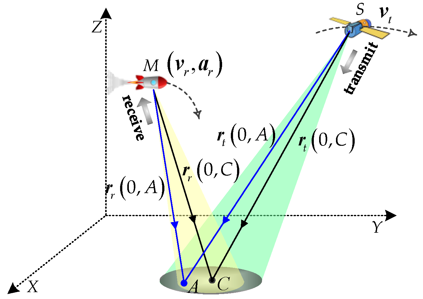
Assume that the frequency modulation chirp pulse is used as the transmitted signal for the ST/MR SAR. Figure 2 shows the ST/MR SAR geometric model. In the coordinate of the imaged scene, point C is the central reference point (CRP) and point A is an arbitrary point on the ground scene. Points S and M are the positions of the transmitter and receiver at aperture center moment (ACM), respectively. and are respectively the transmitter and receiver velocity vectors and is the acceleration vector of the missile-borne receiver. In this paper, ‘t’ and ‘r’ denote the transmitter and receiver, respectively. After reviewing the studies in the available literature [9,10,16,38,39,40,41,42,43], we integrate the important results and then show that the flight path of spaceborne SAR can be equivalent to a curved path, which is mainly caused by the curved orbit and the rotating planetary surface and the flight path of the missile can be described by using the motion parameters, including the velocity, acceleration, and higher-order parameters, obtained from the information provided by the inertial navigation system (INS). According to the imaging geometry, the instantaneous slant range of the point A is expressed as:
where and are the slant range vectors of the transmitter and receiver, respectively, to point A at ACM; is the azimuth time; and is the absolute operator. In this work, the symbols ‘A’ and ‘C’ denote the arbitrary target A and the reference target C, respectively. Particularly, the higher-order motion parameters of the satellite and the missile are not included in this work because they have no impact on the image qualities, which have been analyzed in Appendix A. One way to treat the complex range history is to expand it in a power series in azimuth time as:
where are expanded coefficients of , which are expressed in Appendix A.
2.2. Flight-Path Constraint
A key factor in determining the imaging performance of the BiSAR is the spatial resolution, which we can also say is the acquisition geometry, including the positions and velocities of both the transmitter and the receiver. This is because it determines the spatial resolution [44]. In this part, the flight-path constraint of the ST/MR SAR characterized by arbitrary configurations is analyzed. The application of vector methods to physical problems most frequently takes the form of differential operations. According to the definition of the gradient operator , the rates of changes of and in the directions of range and azimuth are equal to and , respectively. Accordingly, the ground space can be spanned by two unit vectors and , which are the projections of and on the ground, respectively. Vectors and are normal to the iso-range and iso-Doppler lines, respectively. Thus, the angle between the iso-range and iso-Doppler lines is derived as:
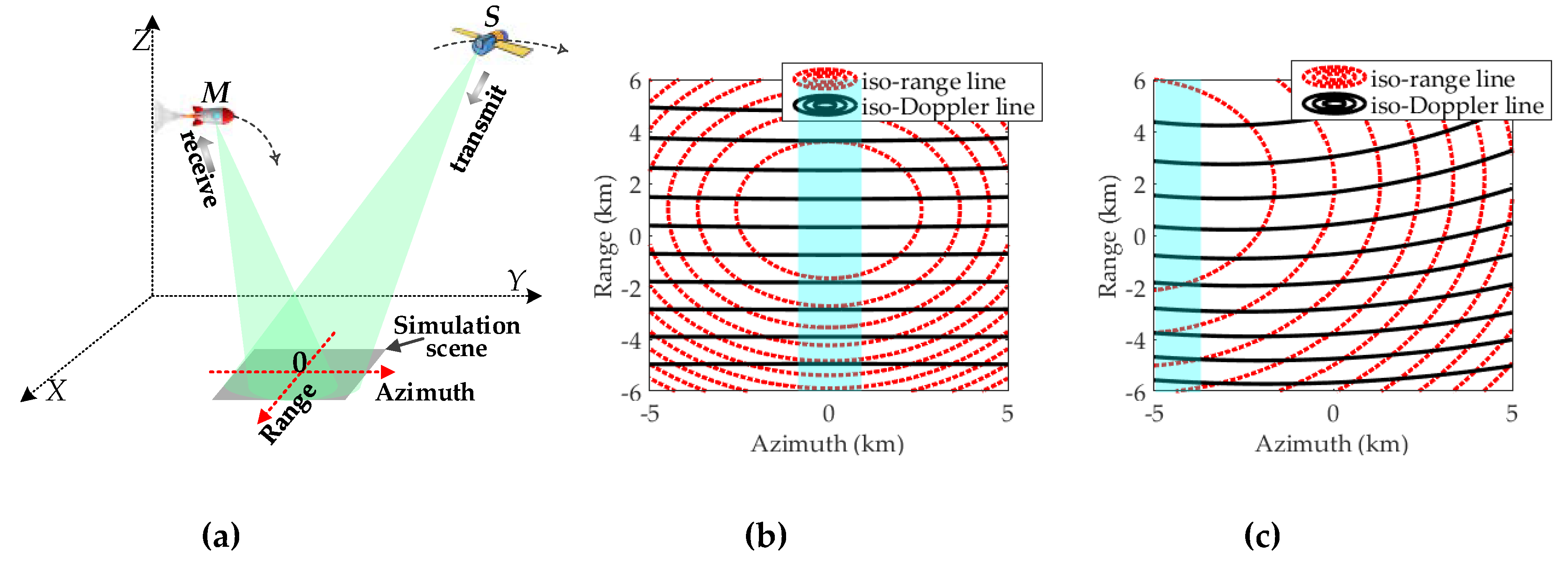
where is the angle between the iso-range and iso-Doppler lines and . The angle in Equation (3) can be used to validate the rationality of the BiSAR geometry. The geometric model is more like that of the broadside monostatic SAR when is close to . Generally, ST/MR SAR with a large has a better geometric structure than that of the ST/MR SAR with a small one. Employing the simulation parameters in Table 1 and the simulation scene shown in Figure 3a, Figure 3b shows the iso-range/iso-Doppler lines by using the parameters of Receiver 1 in Table 1 and Figure 3c is the simulation result by the parameters of Receiver 2. In these figures, the angle between iso-range and iso-Doppler lines of each point on the ground scene can be derived by using Equation (3). Clearly, in the blue area in these two figures, the angles between iso-range and iso-Doppler lines are very small, even close to zero, which means that the cross-couplings between the range and azimuth are extremely serious. Thus, it is difficult to focus the echo data received from these areas.
2.3. Flight-Path Constraint
Traditional methods considering the ‘Stop-Go’ assumption have been widely studied and can be well-applied for the SAR on the high-speed platform [18,19,20]. However, in the case of large maneuvers of the missile, the impacts brought about by the accelerations are beyond consideration. In this part, a new mathematical model is established to describe the ST/MR SAR with a high accuracy.
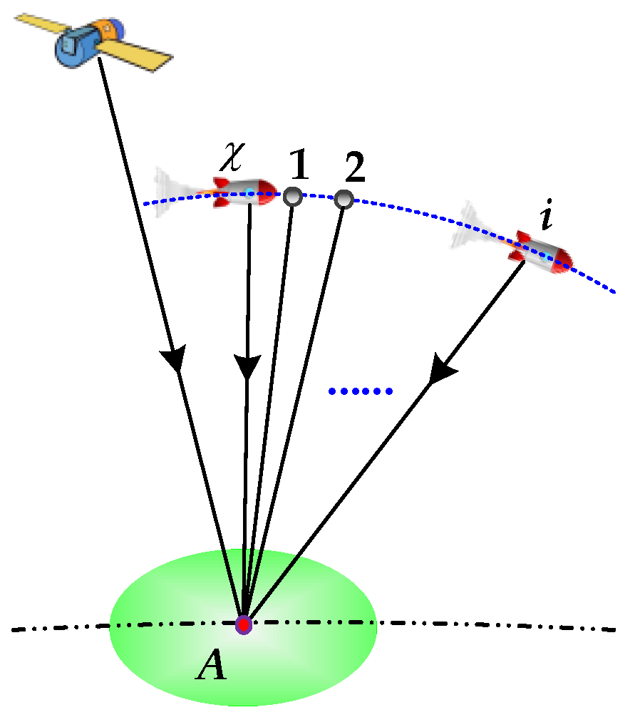
It is generally known that the exact solution of the time delay brought about by the ‘Stop-Go’ assumption is difficult to obtain because of the higher-order transcendental function. To solve this problem, an iterative method is presented to explore an efficient solution. Figure 4 shows the transmitted and received instants, taking the platform movement into account. The radar signal is transmitted by the radar on the satellite at slow time and received by the missile at the position at , as shown in Figure 4, and is a known initial time for the transmission. Thus, the propagation time can be derived as . The basic procedure of the iterative method is listed in Algorithm 1, where is the speed of light, and , , , , and have been defined in Section 2.1. The iterative range history can be regarded as a satisfactory result if the iterative error is less than the error tolerance . The iterative algorithm is applicable for different SAR with maneuvers.
| Algorithm 1. Basic procedure. |
| 1: Fixed input parameters: , , , , , , 2: Initialization (i=0): 3: Iterations (i≥1): 4: Calculate the delay: 5: Calculate the slant range of the receiver: 6: If , return and stop. 7: Calculate the time of the receiver: 8: Set . |
Clearly, the complicated procedure would lead to a complex result and make the focusing algorithm difficult to design. To avoid the cumbersome procedure, a ‘fixed-value’ iterative method is developed. By analyzing the effects brought about by different iterative numbers, we find that the delay time errors tend to the extremely small fixed-values after one time iteration. Thus, using one-time iteration, the new range history can be derived as:
where and are the expansion coefficients which can be found in Appendix B. Employing the simulation parameters in Table 2 and the scene in Figure 3a, Figure 5 shows the comparative results of the residual phase errors. It is noted that the proposed model can be well-applied for the ST/MR SAR, whereas the traditional method cannot because the acceleration is not considered.
3. Imaging Approach
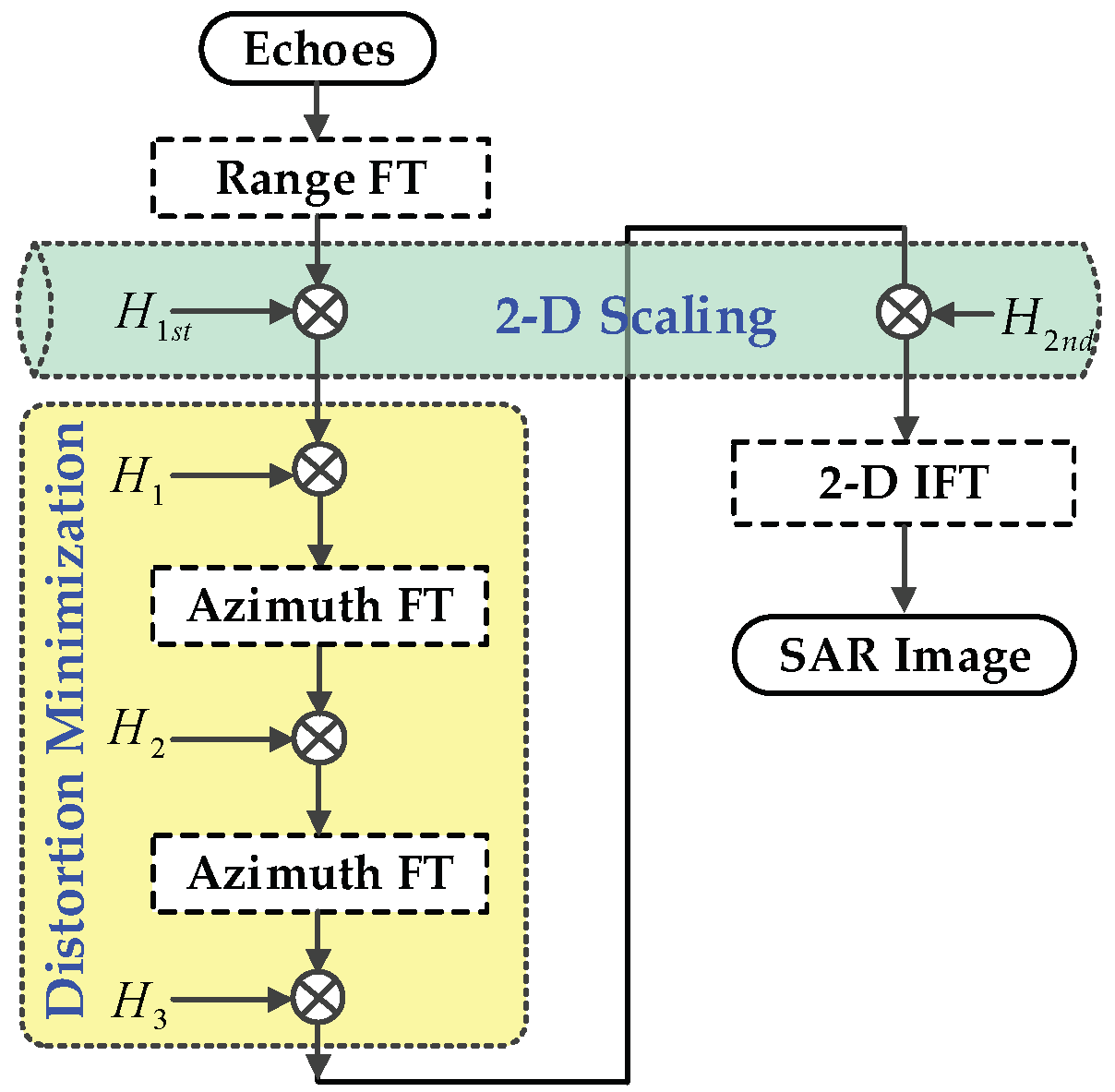
The geometric model is established, and the mathematic model of the ST/MR SAR is derived in Section 2. Based on the accurate model, we concentrate on the corresponding imaging algorithm in this section. A 2-D scaling algorithm is proposed to focus the ST/MR SAR data. The flowchart is shown in Figure 6. Because of the complicated mathematic model, we design the imaging approach performed in the 2-D hybrid domain. Two short remarks will be helpful to understanding the 2-D scaling algorithm:
- ➢
- Cross-couplings. Traditionally, the cross-coupling phases in the 2-D spectrum derived by using the principle of stationary point (POSP) and MSR are divided into two parts, i.e., the range- and azimuth-dependent ones, and they are eliminated separately, which would introduce errors in the final image. The 2-D scaling algorithm in this work can avoid this division and make the processing more accurate than that of the traditional methods.
- ➢
- Spatial variations. Generally, the range, azimuth, and cross-coupling spatial variations in the 2-D spectrum are difficult to be removed simultaneously and entirely because of the complex phase expressions. In the 2-D scaling algorithm, two perturbation functions performed in the hybrid domains can eliminate the range, azimuth, and cross-coupling spatially variant terms simultaneously and entirely, which can avoid the defect of the traditional methods that the range and cross-coupling spatial variations cannot be removed.
3.1. 2-D Scaling in Range Frequency/Azimuth Time Domain
Assume that a linear frequency modulation (LFM) signal is transmitted with the frequency modulation (FM) rate being . After range compression, the received echo signal in the range frequency/azimuth time domain can be expressed as
where and are the range and azimuth windows, respectively; and and are the carrier and range frequencies, respectively. Note that the traditional methods are difficult to apply for the ST/MR SAR case directly because of the complex phase in Equation 5.
In the 2-D scaling algorithm, a perturbation function, performed in the 2-D hybrid domain (hybrid domain between range frequency fr and azimuth time η), is firstly designed to weaken the spatially variant phases and also provides many more DOFs for the echo signal, i.e.,
where the coefficients , , and are all the scaling factors and can be derived at the next step. Multiplying Equation (6) with Equation (5) and ignoring the unimportant amplitudes, one can obtain that
Note that the spatial variations of the high-order terms corresponding to in Equation (7) are generally very small and can be ignored, which indicates that the second phase term can be compensated for by using the bulk compensation function corresponding to the reference target. Then, the echo signal can be expressed as
3.2. Distortion Minimization
After perturbation processing, the echo signal is transformed into the 2-D spectrum. Of particular note is the spectral distortion and aliasing after azimuth Fourier transform (FT). Three main uncertainty factors should be faced and they could greatly deteriorate the final image if we do not pay attention to them:
- ➢
- ➢
- ➢
- After multiplying Equation (6) with echoes, the rate of the Doppler FM becomes , which means that the azimuth bandwidth may display a big change. Thus, the possible spectral distortion should be eliminated before the azimuth FT of the signal.
The spectral aliasing elimination method has been discussed in [48] in detail and one can use it for efficient data processing. The processes include the deramping function , compensation function , and quadratic function [48]. The only difference is that the original Doppler FM should be substituted by so that the spectral distortion and aliasing partly introduced by the perturbation function can be eliminated entirely. Particularly, the spectral aliasing elimination method is an extension of the traditional two-step approach in [49,50], whose essence is the time-frequency rotation. Thus, two azimuth FTs are used. The first one is used as a filter to change the sampling interval and the second one is a normal transformation.
After distortion minimization, the 2-D spectrum of the echo signal is given by
where is the new azimuth frequency corresponding to the new azimuth time after distortion minimization, i.e., and , where is the azimuth frequency before distortion minimization. represents Doppler parameters of the range equation corresponding to A, all of which are spatially variant terms and their expressions can be found in Appendix C. It is important to note that the expressions of the 2-D spectrum before and after distortion minimization are the same, except for and .
3.3. 2-D Scaling in Range Frequency/Azimuth Frequency Domain
The coefficients and are the range and Doppler positions of A, respectively. To obtain the well-focused image, the higher-order terms corresponding to , , and should be removed entirely. In this sub-section, another perturbation function, performed in the 2-D hybrid domain (hybrid domain between range frequency and azimuth frequency ), is presented, i.e.,
where , , and are all the scaling factors similar to those of , , and in Equation (6). After the second perturbation processing by multiplying Equation (10) with Equation (9), the phase terms of the echo signal are derived as
Clearly, the range, azimuth, and cross-coupling spatial variations of A are all included in the third term in Equation (11) and they should be eliminated to guarantee the image qualities. Setting the terms involving the spatially variant coefficients to zero is a crucial operation for the 2-D scaling algorithm, i.e., . According to the detailed expressions in Appendix B, the following equations are obtained:
Clearly, three equations with six unknown scaling factors make it difficult to derive the solutions for Equation (12). To solve this problem, we firstly rewrite Equation 12 as
where , , , , , and . Then, , , and are respectively expanded in the power series with respect to , i.e.,
where , , and are expansion coefficients of , and are the expansion coefficients of , and is the expansion coefficient of , i.e., and . Note that both Equations (13) and (14) are used for the expressions of β2(A), β3(A), and β4(A), but with different formulae. Making use of the similarities and differences between Equations (13) and (14), we can obtain the following six equations with six unknowns ξi, ωi(i = 2, 3, 4), i.e.,
Solving this equation set in Equation (15), we can derive its solutions as
where , , and . After the 2-D scaling processing in the hybrid domain by using Equations (16) and (17), the echo signal can be expressed as
Clearly, the phase in Equation 18 is a 2-D linear one with respect to the range frequency and azimuth frequency . By performing a 2-D inverse FT (IFT) on Equation (18), one can obtain a focused image for ST/MR SAR data. Particularly, without introducing any extra operations, the range, azimuth, and cross-coupling spatially variant terms in Equation (5) can be removed simultaneously and entirely by using the 2-D scaling algorithm, which indicates that the proposed approach could be easy and efficient to implement for the ST/MR SAR data. Next, some discussions are given to facilitate a better understanding of the proposed method.
4. Simulation Results
In this section, some simulation results from the two experiments are shown to validate the proposed method and analysis.
4.1. Case I
In this experiment, the effectiveness of the mathematical model presented in Equation (4) is analyzed and verified. The traditional ‘Stop-Go’ and the non-‘Stop-Go’ models in [20] are compared with the proposed 2-D scaling algorithm. The simulation parameters are listed in Table 2. The ST/MR SAR data are simulated with one reference target PT0 being arranged on the ground scene.
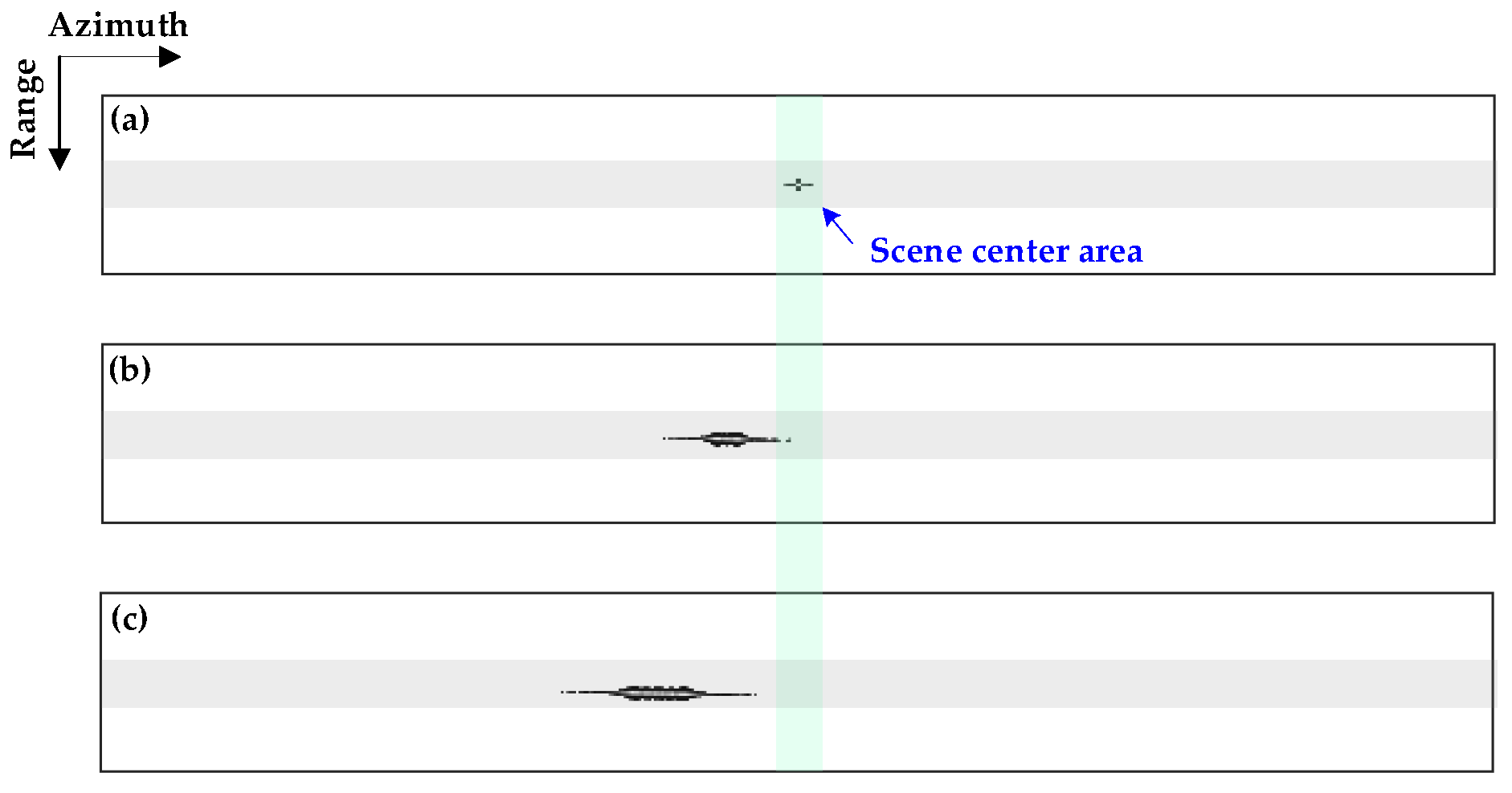
Figure 7a–c show the focused results of the ground scene by the proposed model, the traditional non-‘Stop-Go’ model, and the traditional ‘Stop-Go’ model, respectively. Clearly, considering the negative impacts brought about by the missile’s accelerations, the focused result of the reference target PT0 in Figure 7a is visually well-focused, with the position being the scene center. However, using the traditional non-‘Stop-Go’ and ‘Stop-Go’ models, the imaging results exhibit great deterioration in the azimuth directions with wrong target positions marked on the ground scenes, as shown in Figure 7b,c.
Figure 8 shows the comparative results of the reference targets which are extracted from the simulated results in Figure 7. Clearly, the 2-D impulse response by the proposed model is well-focused with relative clear separations of the main lobe and first and subsequential sidelobes, whereas the ones from the traditional non-‘Stop-Go’ and ‘Stop-Go’ models are defocused completely, which indicates that the impacts of the accelerations on the ‘Stop-Go’ model must be taken into consideration when design the focusing algorithm.
4.2. Case II
In order to verify the effectiveness of the proposed approach, some simulated results are given in this case. The simulated parameters are listed in Table 3. A 3 × 3 dot-matrix is arranged on the simulated ground scene, with center target PT2 being the reference target. The geometry of the scene is presented in Figure 9, with the scene size being 2 km × 2 km.
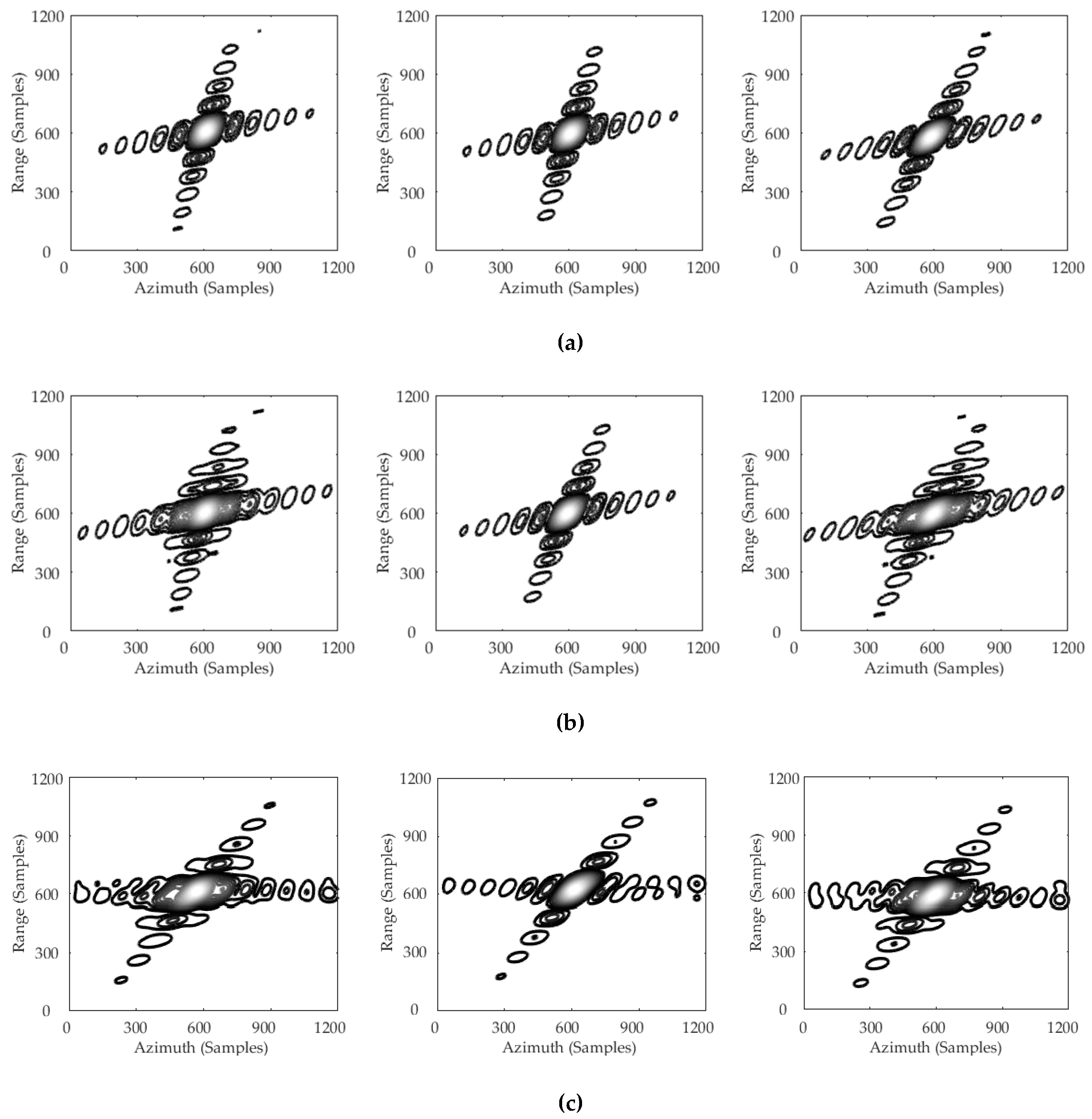
By performing the proposed algorithm, simulated results of targets PT1, PT2, and PT3 are shown in Figure 10a. It can be seen that the main lobe and the side lobes are generally separated, and the center point PT2 and the edge points PT1 and PT3 are all well-focused. For comparisons, the 2-D impulse responses of these three targets obtained by the NCSA [32] and the GPFA [16] are respectively shown in Figure 10b,c. Experimental results indicate that the center points on the ground scene are focused well, whereas the ones on the edges remain highly defocused in the azimuth direction. For the NCSA, the range and cross-coupling spatial variations are not considered and they would lead to great deterioration in the final image. Moreover, the residual phases after NCSA, eliminated by the deramping function, would also introduce errors in the imaging result. The GPFA can be used for the ST/MR SAR; however, its depth of field is greatly affected by the wavefront curvature.
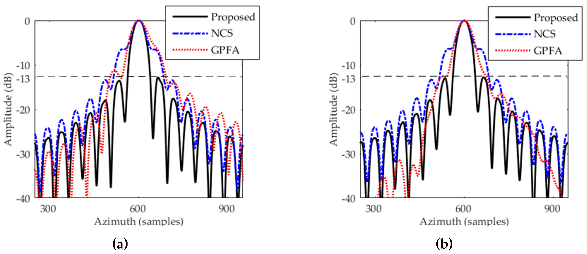
The profiles of azimuth spread functions of targets PT1 and PT3 are presented in Figure 11. To quantify the precision of the proposed approach, the impulse-response width (IRW), peak sidelobe ratio (PSLR), and integrated sidelobe ratio (ISLR) are also used as criteria. The results are listed in Table 4. The proposed method is noted to be generally acceptable. Moreover, to further elevate the performance of the 2-D scaling algorithm, the position errors are computed in this part. The deviations of point targets PT1, PT2, and PT3 from their ideal values are 0.912 m, 0.475 m, and 1.016 m, respectively. Clearly, the deviations were generally within or around one IRW. Consequently, with the incorporation of 2-D perturbations and distortion minimization, promising results are obtained for the ST/MR SAR.
5. Discussion
5.1. 2-D Range Compression
Antenna motion during the transmission and reception of a pulse causes pulse distortion and is analogous to the familiar Doppler frequency shift associated with sound waves [1]. Typically, the phase effect of motion during a pulse is small, but this effect can be become significant as pulse lengths increase and motion becomes faster. Employing the simulation parameters in Table 2, the phase error brought about by the motion during transmission and reception of a pulse is about 3.73 and the extra phase error brought about by the acceleration term is about 0.007, which indicates that the effect of the motion during transmission and reception should be considered, whereas the impact by the acceleration can be ignored. Actually, the effect has been already discussed in [18,19,20]. Based on the analytical derivations in [19,20], the effect can be compensated by
Multiplying Equation (19) by the range compression function in the range frequency domain, the range compression together with the effect compensation (in this work, we call it the 2-D range compression operation) can be expressed as
5.2. Computational Load
The computational load is analyzed in this section. In the 2-D scaling algorithm, two range FTs, three azimuth FTs, and four multiplications are utilized. The computational load can be derived as , where and are the numbers of range and azimuth samples, respectively. In comparison, for the BPA (e.g., [35]), for each pixel in the final image, a signal vector with a length is extracted from range compressed data, multiplied with a phase function, and summed; thus, the total computational load can be expressed as . In a standard CSA (e.g., [51]), two range FTs, one azimuth FT, and three multiplications are used. Therefore, the computational load can be expressed as .
Clearly, the BPA has the highest computational load. The load of the 2-D scaling algorithm is slightly heavier than that of the CSA. Ratios at five sample sizes of both range and azimuth are computed to quantify the comparison (Table 5).
6. Conclusions
In this paper, a new BiSAR imaging configuration is presented, with the satellite being the transmitter and missile being the receiver. This system could provide many advantages, including wide coverage, unrestricted geography, low detection probability of the missile, and forward-looking imaging. A geometric model for the ST/MR SAR is first established by using motion parameter vectors and the flight-path constraint is derived, and the corresponding focusing approach is then proposed. In this approach, two perturbation functions are designed in the 2-D hybrid domain to eliminate the range, azimuth, and cross-coupling spatially variant terms in the ST/MR data and distortion minimization is applied to avoid the possible spectral distortion and aliasing in the 2-D spectrum. Furthermore, discussions including the 2-D range compression and the computational load are studied. Validity and applicability are studied through theoretical analysis and numerical experiments.
Author Contributions
S.T. conceived the main idea; P.G. and L.Z. conceived and designed the experiments; S.T. and P.G. analyzed the data and wrote the paper; S.T. revised this paper.
Acknowledgments
This work was supported in part by the National Natural Science Foundation of China under Grants 61701393, 61601343, and 61671361; in part by China Postdoctoral Science Foundation Funded Project under Grant 2016M600768; in part by the National Natural Science Foundation of the Shaanxi Province under Grant 2018JM6054; in part by the Postdoctoral Research Project Foundation of the Shaanxi Province; and in part by the National Defense Foundation of China. The authors would like to thank the Hing Cheung So for his useful comments and suggestions, which were of great help in improving this paper.
Conflicts of Interest
The authors declare no conflict of interest.
Appendix A
In this Appendix, the coefficients of the Taylor series are listed as
where and in Table A1 are the Taylor series expansion coefficients of the range histories corresponding to the transmitter and the receiver, respectively. is the inner operator. Thus, the coefficients are derived as .

Table A1.
Coefficients of Taylor series expansion.
| Coefficient | Transmitter | Coefficients | Receiver |
|---|---|---|---|
Considering the high-order accelerations, the range history of A can be expressed as
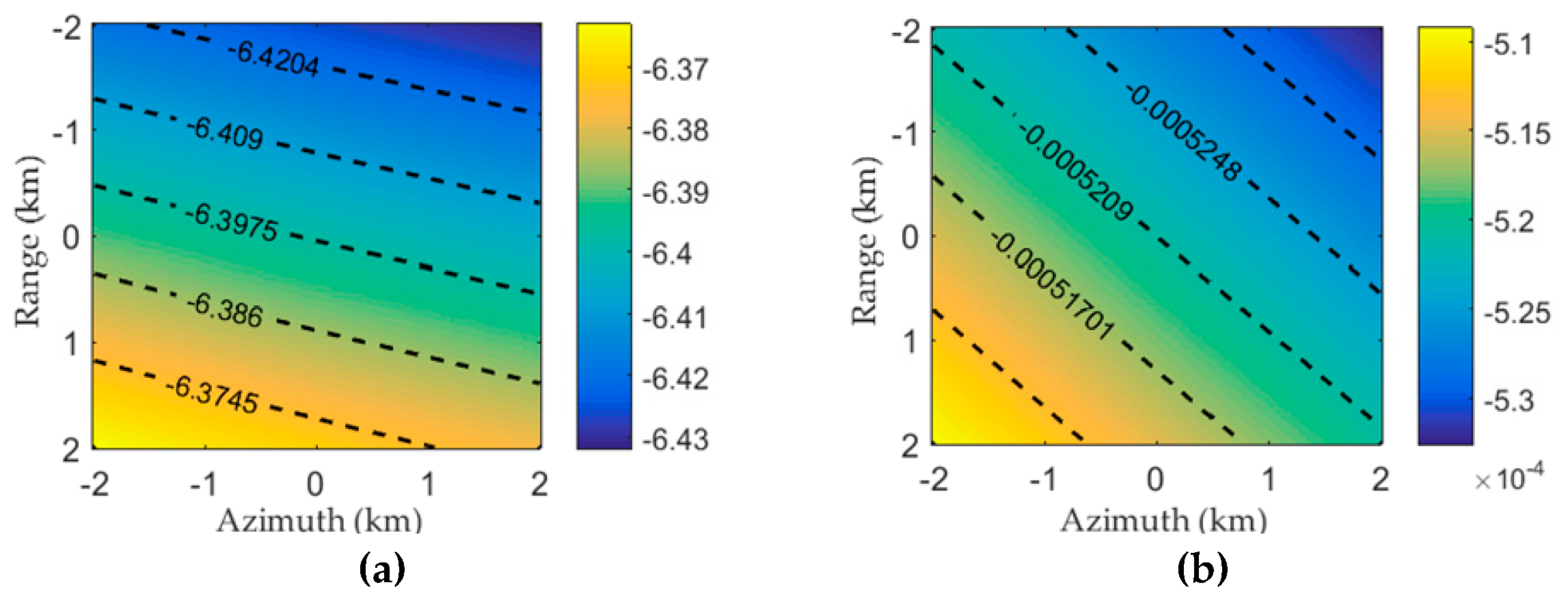
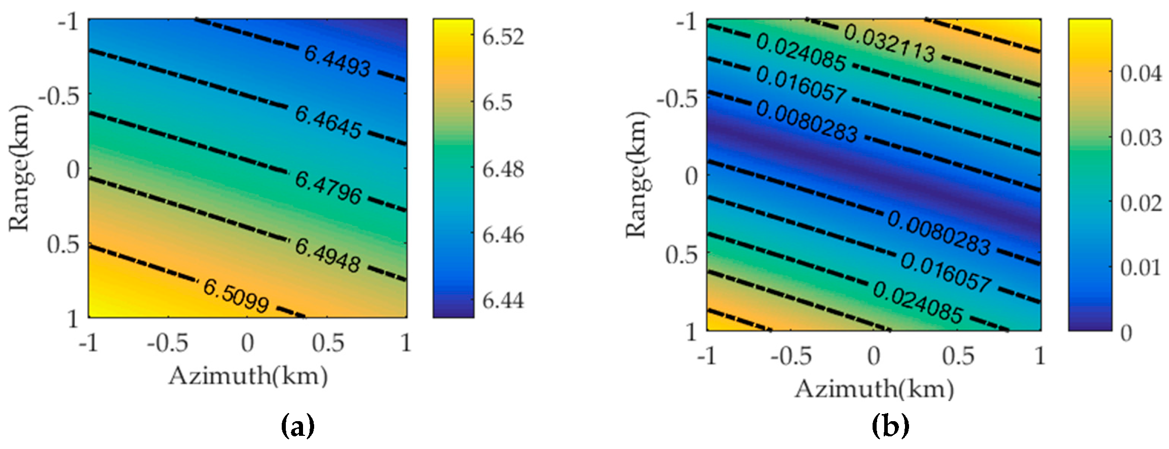
where , , and are the second-, third-, and fourth- order accelerations of the transmitter, respectively. and are the third- and fourth-order accelerations of the receiver, respectively. Employing the simulated parameters in Table 2 and Equation (A1), Figure A1 shows the residual errors brought about by the high-order motion parameters. The unit of the contour maps is . Clearly, the bulk phase errors are all larger than , whereas the spatially variant ones are all far less than , which indicates that the high-order motion parameters can be compensated by without considering the spatial variations and they have no impact on the focusing algorithm design.
Figure A1.
Residual errors: (a) Bulk phase errors. (b) Spatially variant errors.

Appendix B
By using the Taylor series expansion in Equation (2), the time delay can be expressed as
where . For the slant range history of the receiver, it can be rewritten as:
where , , , and are the equivalent slant range, velocity, acceleration, and rate of acceleration vectors, respectively, and they are given by , , , , and .
According to the previous derivations in Equations (B1) and (B2), the slant range history of the ST/MR SAR can be expressed as
where in Equation (B3) and are the expansion coefficients of .
Appendix C
References
- Ender, J.H.; Walterscheid, I.; Brennner, A. New Aspects of Bistatic SAR: Processing and Experiments. Proc. IGARSS 2004, 9, 1758–1762. [Google Scholar]
- Loffeld, O.; Nies, H.; Peters, V.; Knedlik, S. Models and Useful Relations for Bistatic SAR Processing. IEEE Trans. Geosci. Remote Sens. 2004, 10, 2031–2038. [Google Scholar] [CrossRef]
- Wu, J.; Sun, Z.; Li, Z.; Huang, Y.; Yang, J.; Liu, Z. Focusing Translational Variant Bistatic Forward-Looking SAR Using Keystone Transform and Extended Nonlinear Chirp Scaling. Remote Sens. 2016, 8, 840. [Google Scholar] [CrossRef]
- Nies, H.; Loffeld, O.; Natroshvili, K. Analysis and Focusing of Bistatic Airborne SAR Data. IEEE Trans. Geosci. Remote Sens. 2007, 11, 3342–3349. [Google Scholar] [CrossRef]
- Rodriguez-Cassola, M.; Prats, P.; Schulze, D.; Tous-Ramon, N.; Steinbrecher, U.; Marotti, L.; Nannini, M.; Younis, M.; Lopez-Dekker, P.; López-Dekker, P.; et al. First Bistatic Spaceborne SAR Experiments with TanDEM-X. Proc. IGARSS 2011, 7, 1393–1396. [Google Scholar]
- Buckreuss, S.; Schattler, B.; Fritz, T.; Mittermayer, J.; Kahle, R.; Maurer, E.; Boer, J.; Bachmann, M.; Mrowka, F.; Schwarz, E.; et al. TenYears of TerraSAR-X Operations. Remote Sens. 2018, 6, 873. [Google Scholar] [CrossRef]
- Espeter, T.; Walterscheid, I.; Klare, J.; Ender, J.H.G. Synchronization Techniques for the Bistatic Spaceborne/Airborne SAR Experiment with TerraSAR-X and PAMIR. Proc. IGARSS 2007, 7, 2160–2163. [Google Scholar]
- Walterscheid, I.; Espeter, T.; Brenner, A.R.; Klare, J.; Ender, J.H.G.; Nies, H.; Wang, R.; Loffeld, O. Bistatic SAR Experiments with PAMIR and TerraSAR-X Setup, Processing, and Image Results. IEEE Trans. Geosci. Remote Sens. 2010, 8, 3268–3279. [Google Scholar] [CrossRef]
- Saeedi, J. Feasibility Study and Conceptual Design of Missile-Borne Synthetic Aperture Radar. IEEE Trans. Syst. Man Cybern. Syst. 2018. in Press. [Google Scholar] [CrossRef]
- Tang, S.; Zhang, L.; Guo, P.; Zhao, Y. An Omega-K Algorithm for Highly Squinted Missile-Borne SAR With Constant Acceleration. IEEE Geosci. Remote Sens. Lett. 2014, 9, 1569–1573. [Google Scholar] [CrossRef]
- Li, Y.; Meng, Z.; Xing, M.; Bao, Z. Configuration Study of Missile-borne Bistatic Forward-looking SAR. Proc. ChinaSIP 2014, 7, 184–188. [Google Scholar]
- Moreira, A. A Golden Age for Spaceborne SAR Systems. Proc. ICMRWC 2014, 1–4. [Google Scholar]
- Li, T.; Chen, K.; Jin, M. Analysis and Simulation on Imaging Performance of Backward and Forward Bistatic Synthetic Aperture Radar. Remote Sens. 2018, 11, 1676. [Google Scholar] [CrossRef]
- Jun, S.; Zhang, X.; Yang, J. Principle and Methods on Bistatic SAR Signal Processing via Time Correlation. IEEE Geosci. Remote Sens. 2008, 10, 3163–3178. [Google Scholar] [CrossRef]
- Walterscheid, I.; Ender, J.H.G.; Brenner, A.R.; Loffeld, O. Bistatic SAR Processing and Experiments. IEEE Geosci. Remote Sens. 2006, 10, 2710–2717. [Google Scholar] [CrossRef]
- Tang, S.; Deng, H.; Guo, P.; Li, Y.; Zhang, L. Generalized PFA for Air-Missile Borne Bistatic Forward-Looking Beam-Steering SAR With Accelerations. IEEE Access. 2019, 1, 74616–74627. [Google Scholar] [CrossRef]
- Meng, Z.; Li, Y.; Xing, M.; Bao, Z. Imaging of Missile-borne Bistatic Forward-looking SAR. Proc. ChinaSIP 2014, 7, 179–183. [Google Scholar]
- Meta, A.; Hoogeboom, P.; Lighthart, L.P. Signal Processing for FMCW SAR. IEEE Trans. Geosci. Remote Sens. 2007, 11, 3519–3532. [Google Scholar] [CrossRef]
- Curlander, J.C.; McDonough, R.N. Synthetic Aperture Radar: System and Signal Processing; Willey: New York, NY, USA, 1991. [Google Scholar]
- Liu, Y.; Xing, M.; Sun, G.; Lv, X.; Bao, Z.; Hong, W.; Wu, Y. Echo Model Analyses and Imaging Algorithm for High-resolution SAR on High-speed Platform. IEEE Trans. Geosci. Remote Sens. 2012, 3, 933–950. [Google Scholar] [CrossRef]
- Yan, H.; Wang, Y.; Yu, H.; Li, L. An Imaging Method of Distributed Small Satellites Bistatic SAR Based on Range Distance Compensation. J. Electron. Inf. Technol. 2005, 5, 771–774. [Google Scholar]
- Qiu, X.; Hu, D.; Ding, C. Focusing Bistatic Images use RDA based on Hyperbolic Approximating. Proc. Int. Conf. Radar, CIE 2006, 1323–1326. [Google Scholar]
- Neo, Y.L.; Wong, F.; Cumming, I.G. A Two-dimensional Spectrum for Bistatic SAR Processing using Series Reversion. IEEE Geosci. Remote Sens. Lett. 2007, 1, 93–96. [Google Scholar] [CrossRef]
- Bamler, R.; Boerner, E. On the Use of Numerically Computed Transfer Functions for Processing of Data from Bistatic SARs and High Squint Orbital SARs. Proc. IGARSS 2005, 2, 1051–1055. [Google Scholar]
- Bamler, R.; Meyer, R.; Liebhart, L. No math: Bistatic SAR Processing Using Numerically Computed Transfer Functions. Proc. IGARSS 2006, 1844–1847. [Google Scholar]
- Neo, Y.L.; Wong, F.H.; Cumming, I.G. Processing of Azimuth-invariant Bistatic SAR Data using the Range Doppler Algorithm. IEEE Geosci. Remote Sens. 2008, 1, 14–21. [Google Scholar] [CrossRef]
- Wang, R.; Deng, Y.K.; Loffeld, O.; Nies, H.; Walterscheid, I.; Espeter, T.; Klare, J.; Ender, J.H.G. Processing the Azimuth-variant Bistatic SAR Data by using Monostatic Imaging Algorithms based on Two-dimensional Principle of Stationary Phase. IEEE Geosci. Remote Sens. 2011, 10, 3504–3520. [Google Scholar] [CrossRef]
- Li, Y.; Zhang, Z.; Xing, M.; Bao, Z. Bistatic Spotlight SAR Processing using the Frequency-scaling Algorithm. IEEE Geosci. Remote Sens. Lett. 2008, 1, 48–52. [Google Scholar] [CrossRef]
- Liu, B.; Wang, T.; Wu, Q.; Bao, Z. Bistatic SAR Data Focusing using an Omega-K Algorithm based on Method of Series Reversion. IEEE Geosci. Remote Sens. 2009, 8, 2899–2912. [Google Scholar]
- Zhong, H.; Liu, X. An Extended Nonlinear Chirp-scaling Algorithm for Focusing Large-baseline Azimuth-invariant Bistatic SAR Data. IEEE Geosci. Remote Sens. Lett. 2009, 3, 548–552. [Google Scholar] [CrossRef]
- Qiu, X.; Hu, D.; Ding, C. An Improved NLCS Algorithm with Capability Analysis for One-stationary BiSAR. IEEE Geosci. Remote Sens. 2008, 10, 3179–3186. [Google Scholar] [CrossRef]
- Zhang, Q.; Wu, J.; Yang, J.; Huang, Y.; Du, K.; Yang, G. Extended Nonlinear Chirp Scaling Algorithm with Topography Compensation for Manueuvering-platform Bistatic Forward-looking SAR. Proc. IGARSS 2017, 1047–1050. [Google Scholar]
- Peng, X.; Wang, Y.; Hong, W.; Wu, Y. Autonomous Navigation Airborne Forward-Looking SAR High Precision Imaging with Combination of Pseudo-Polar Formatting and Overlapped Sub-Aperture Algorithm. Remote Sens. 2013, 11, 6063–6078. [Google Scholar] [CrossRef]
- Carrara, W.G.; Goodman, R.S.; Ricoy, M.A. New Algorithms for Widefield SAR Image Formation. Proc. Radar Conf. 2004, 38–43. [Google Scholar]
- Rodriguez-Cassola, M.; Parts, P.; Krieger, G.; Moreira, A. Efficient Time-domain Image Formation with Precise Topography Accommodation for General Bistatic SAR Configurations. IEEE Trans. Aerosp. Electron. Syst. 2011, 4, 2949–2966. [Google Scholar] [CrossRef]
- Lin, C.; Tang, S.; Zhang, L.; Guo, P. Focusing High-Resolution Airborne SAR with Topography Variations Using an Extended BPA Based on a Time/Frequency Rotation Principle. Remote Sens. 2018, 8, 1275. [Google Scholar] [CrossRef]
- Yang, L.; Zhou, S.; Zhao, L.; Xing, M. Coherent Auto-Calibration of APE and NsRCM under Fast Back-Projection Image Formation for Airborne SAR Imaging in Highly-Squint Angle. Remote Sens. 2018, 10, 321. [Google Scholar] [CrossRef]
- Eldhuset, K. Ultra high resolution spaceborne SAR processing with EETF4. Proc. IEEE IGARSS 2001, 7, 2689–2691. [Google Scholar]
- Wu, C.; Liu, K.Y.; Jin, M. Modeling and a correlation algorithm for spaceborne SAR signals. IEEE Trans. Aerosp. Electron. Syst. 1982, 5, 563–575. [Google Scholar] [CrossRef]
- Mims, J.H.; Farrell, J.L. Synthetic Aperture Imaging with Maneuvers. IEEE Trans. Aerosp. Electron. Syst. 1972, 4, 410–418. [Google Scholar] [CrossRef]
- Wang, P.; Liu, W.; Chen, J.; Niu, M.; Yang, W. A High-order Imaging Algorithm for High-resolution Spaceborne SAR Based on a Modified Equivalent Squint Range Model. IEEE Trans. Geosci. Remote Sens. 2015, 3, 1225–1235. [Google Scholar] [CrossRef]
- Bao, M.; Xing, M.; Li, Y.; Wang, Y. Two-dimensional Spectrum for MEO SAR Processing using a Modified Advanced Hyperbolic Range Equation. Electronic Lett. 2011, 8, 1043–1045. [Google Scholar] [CrossRef]
- Tobin, M.; Greenspan, M. Smuggling Interdiction using an Adaptation of the AN/APG-76 Multimode Radar. IEEE Aerosp. Electron. Syst. Mag. 1996, 11, 19–24. [Google Scholar] [CrossRef]
- Moccia, A.; Renga, A. Spatial Resolution of Bistatic Synthetic Aperture Radar: Impact of Acquisition Geometry on Imaging Performance. IEEE Trans. Geosci. Remote Sens. 2011, 10, 3487–3503. [Google Scholar] [CrossRef]
- Lanari, R.; Tesauro, M.; Sansosti, E.; Fornaro, G. Spotlight SAR Data Focusing based on a Two-step Processing Approach. IEEE Trans. Geosci. Remote Sens. 2001, 9, 1993–2004. [Google Scholar] [CrossRef]
- Lanari, R.; Zoffoli, S.; Sansosti, E.; Fornaro, G.; Serafino, F. New Approach for Hybrid Strip-map/spotlight SAR Data Focusing. Proc. Inst. Elect. Eng.-Radar Sonar Navig. 2001, 6, 363–372. [Google Scholar] [CrossRef]
- Tang, S.; Zhang, L.; Guo, P.; Liu, G.; Sun, G.-C. Acceleration Model Analyses and Imaging Algorithm for Highly Squinted Airborne Spotlight Mode SAR with Maneuvers. IEEE J. Sel. Topics Appl. Earth Observat. Remote Sens. 2015, 3, 1120–1131. [Google Scholar] [CrossRef]
- Tang, S.; Zhang, L.; Guo, P.; Liu, G.; Zhang, Y.; Li, Q.; Gu, Y.; Lin, C. Processing of Monostatic SAR Data with General Configurations. IEEE Trans. Geosci. Remote Sens. 2012, 9, 3595–3609. [Google Scholar] [CrossRef]
- Lanari, R.; Tesauro, M.; Sansosti, E.; Fornaro, G. Spotlight SAR Data Focusing Based on a Two-step Processing Approach. IEEE Trans. Geosci. Remote Sens. 2001, 9, 1993–2004. [Google Scholar] [CrossRef]
- Lanari, R.; Zoffoli, S.; Sansosti, E.; Fornaro, G.; Serafino, F. New Approach for Hybrid Strip-map/spotlight SAR Data Focusing. Proc. Inst. Elect. Eng.-Radar Sonar Navig. 2001, 6, 363–372. [Google Scholar] [CrossRef]
- Raney, R.K.; Runge, H.; Bamler, R.; Cumming, I.G.; Wong, F.H. Precision SAR Processing using Chirp Scaling. IEEE Trans. Geosci. Remote Sens. 1994, 4, 786–799. [Google Scholar] [CrossRef]
Figure 1.
BiSAR mounted on different platforms.

Figure 2.
ST/MR SAR geometric model.

Figure 3.
Simulation experiment. (a) Simulation scene. (b) Simulation result by parameters of Receiver 1. (c) Simulation result by parameters of Receiver 2.
Figure 3.
Simulation experiment. (a) Simulation scene. (b) Simulation result by parameters of Receiver 1. (c) Simulation result by parameters of Receiver 2.

Figure 4.
Iterative procedure.

Figure 5.
Residual phase errors. (a) Traditional non-‘Stop-Go’ model. (b) Proposed model.

Figure 6.
Block diagram of the imaging approach.

Figure 7.
Simulation results. (a) Proposed model. (b) Traditional non-‘Stop-Go’ model. (c) Traditional ‘Stop-Go’ model.
Figure 7.
Simulation results. (a) Proposed model. (b) Traditional non-‘Stop-Go’ model. (c) Traditional ‘Stop-Go’ model.

Figure 8.
2-D impulse response of the reference target. (a) Proposed model. (b) Traditional non-‘Stop-Go’ model. (c) Traditional ‘Stop-Go’ model.
Figure 8.
2-D impulse response of the reference target. (a) Proposed model. (b) Traditional non-‘Stop-Go’ model. (c) Traditional ‘Stop-Go’ model.

Figure 9.
Ground scene for simulation.

Figure 10.
Comparative results of targets PT1, PT2, and PT3. (a) Proposed. (b) NCSA. (c) GPFA.

Figure 11.
Azimuth profiles by the proposed method, NCSA, and GPFA. (a) Target PT1. (b) Target PT3.

Table 1.
Parameter settings.
| Platform | Transmitter | Receiver 1 | Receiver 2 | |
|---|---|---|---|---|
| Parameter | ||||
| Radar Position at ACM | (0, 1000, 500) km | (12.5, −4, 25) km | (−6, −4, 30) km | |
| Velocity Vector | (0, 7600, 0) m/s | (0, 1000, 0) m/s | (−100, −1200, 800) m/s | |
| Acceleration Vector | / | (10, −30, −50) m/s2 | (50, −60, −35) m/s2 | |
| Elevation Angle | 84.1° | 45.8° | 32.3° | |
Table 2.
Parameter settings for Case I.
| Platform | Transmitter | Receiver | |
|---|---|---|---|
| Parameter | |||
| Radar Position at ACM | (0, 0, 754) km | (132, 0, 15) km | |
| Velocity Vector | (0, 7600, 0) m/s | (300, 1200, −200) m/s | |
| Acceleration Vector | / | (30, 54, −26) m/s2 | |
| Elevation Angle | 74.1° | 44.6° | |
| Carrier Frequency | 9.65 GHz | ||
| Pulse Width | 20 μs | ||
| Pulse Bandwidth | 200 MHz | ||
| Sampling Frequency | 300 MHz | ||
| Azimuth Resolution | 0.823 m | ||
Table 3.
Parameter settings for Case II.
| Platform | Transmitter | Receiver | |
|---|---|---|---|
| Parameter | |||
| Radar Position at ACM | (0, 0, 510) km | (112, −78, 25) km | |
| Velocity Vector | (0, 7600, 0) m/s | (−170, 800, −640) m/s | |
| Acceleration Vector | / | (13, −34, −68) m/s2 | |
| Elevation Angle | 81.3° | 27.7° | |
| Carrier Frequency | 9.65 GHz | ||
| Pulse Width | 20 μs | ||
| Pulse Bandwidth | 240 MHz | ||
| Sampling Frequency | 360 MHz | ||
| Azimuth Resolution | 0.716 | ||
Table 4.
Image quality parameters.
| Range | Azimuth | ||||||
|---|---|---|---|---|---|---|---|
| Method | Target | IRW (m) | PSLR (dB) | ISLR (dB) | IRW (m) | PSLR (dB) | ISLR (dB) |
| Proposed | PT1 | 0.626 | −13.21 | −9.97 | 0.723 | −13.09 | −9.91 |
| PT3 | 0.625 | −13.19 | −10.01 | 0.712 | −13.04 | −9.84 | |
| NCSA | PT1 | 0.625 | −13.20 | −9.99 | 0.983 | −7.04 | −7.36 |
| PT3 | 0.627 | −13.18 | −9.98 | 0.965 | −6.83 | −7.28 | |
| GPFA | PT1 | 0.626 | −13.20 | −10.02 | 1.124 | −10.12 | −8.07 |
| PT3 | 0.628 | −13.19 | −9.99 | 1.059 | −12.25 | −6.63 | |
Table 5.
Computational load analysis.
| Data Size in Samples (×103) | 1 | 2 | 4 | 8 | 16 |
|---|---|---|---|---|---|
| CSA/Proposed | 0.793 | 0.794 | 0.794 | 0.795 | 0.795 |
| BPA/Proposed | 35.59 | 91.25 | 194.81 | 387.78 | 750.61 |
© 2019 by the authors. Licensee MDPI, Basel, Switzerland. This article is an open access article distributed under the terms and conditions of the Creative Commons Attribution (CC BY) license (http://creativecommons.org/licenses/by/4.0/).
Share and Cite
MDPI and ACS Style
Tang, S.; Guo, P.; Zhang, L.; Lin, C. Modeling and Precise Processing for Spaceborne Transmitter/Missile-Borne Receiver SAR Signals. Remote Sens. 2019, 11, 346. https://0-doi-org.brum.beds.ac.uk/10.3390/rs11030346
AMA Style
Tang S, Guo P, Zhang L, Lin C. Modeling and Precise Processing for Spaceborne Transmitter/Missile-Borne Receiver SAR Signals. Remote Sensing. 2019; 11(3):346. https://0-doi-org.brum.beds.ac.uk/10.3390/rs11030346
Chicago/Turabian StyleTang, Shiyang, Ping Guo, Linrang Zhang, and Chunhui Lin. 2019. "Modeling and Precise Processing for Spaceborne Transmitter/Missile-Borne Receiver SAR Signals" Remote Sensing 11, no. 3: 346. https://0-doi-org.brum.beds.ac.uk/10.3390/rs11030346
Note that from the first issue of 2016, this journal uses article numbers instead of page numbers. See further details here.