This section starts with the performance of multi-GNSS PPP time transfer with different precise products released by GFZ and CODE, as well as the advantage of multi-GNSS PPP with respect to a single satellite system. Following that is an evaluation of multi-GNSS PPP time transfer with a between-epoch constraint model with respect to that with a white noise model.
4.1. Multi-GNSS PPP Time Transfer with Different Precise Products
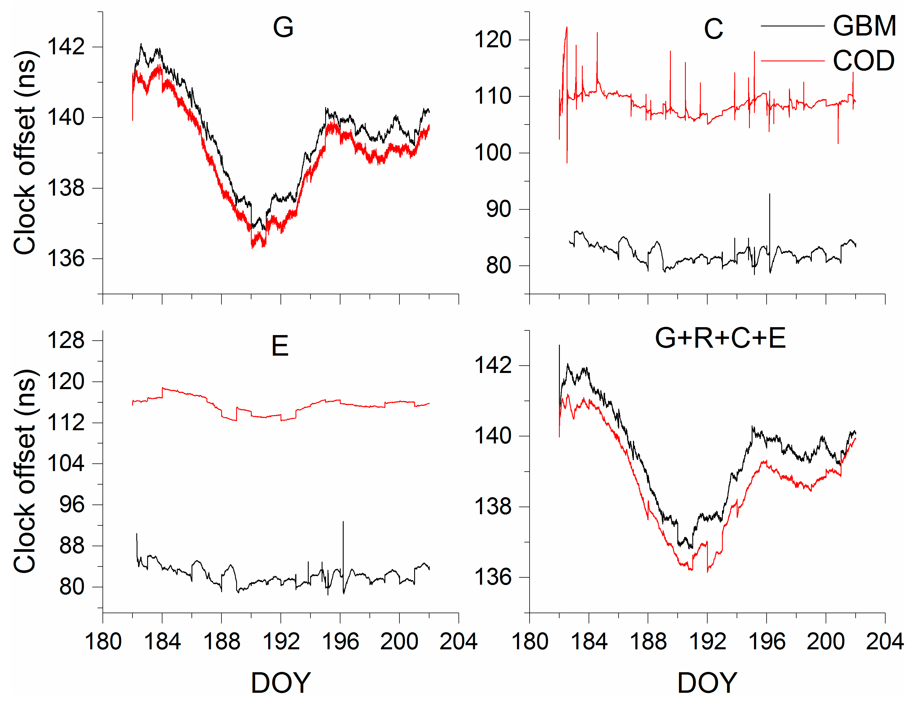
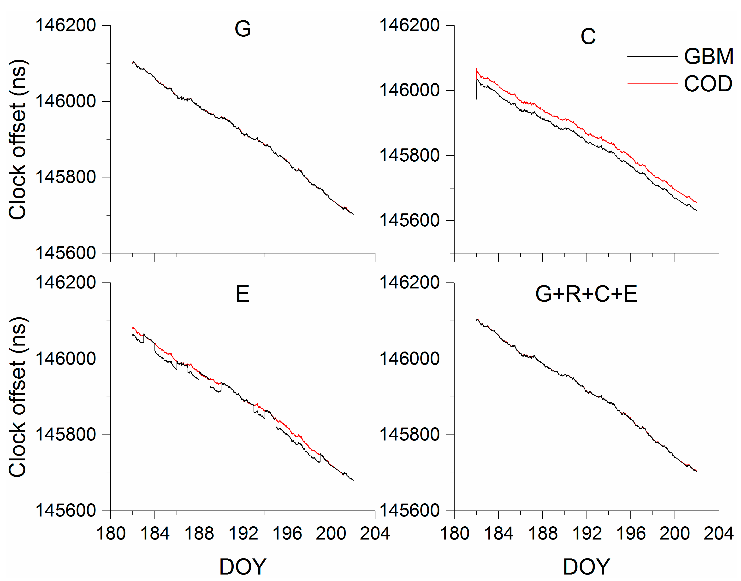
As an example, we show in
Figure 2 the clock offsets for single- and multi-GNSS models on BRUX using GBM and COD products. Furthermore, the clock offsets for single- and multi-GNSS models on HARB using GBM and CODE products are displayed in
Figure 3. These results suggest four findings.
First, the results of GPS-only, BDS-only, Galileo-only, and multi-GNSS PPP using GBM and COD products present a system bias, which is evidenced by the fact that the reference times of GBM and COD products are different. Although the reference time of different products is not the same, the accuracy of time transfer is not affected because the reference time is eliminated. In addition, GPS and BDS PPP solutions with the same products also show a system bias, which is evidenced by the fact that a hardware delay is related to the signals and absorbed by the receiver clock offset. Second, the clock offsets of BDS-only and Galileo-only PPP using GBM and COD products all show an apparent jump at each day, while GPS PPP solutions do not. This may be explained by the fact that the reference times of BDS-only and Galileo-only products in GBM and COD are not aligned to GPST or a unified time scale. Third, BDS PPP solutions using GBM products perform better than those using COD products. The reason is that COD products have no GEO satellite orbit or clock products. Additionally, the performance of GPS-only PPP is better than that of BDS-only PPP at the Eurasian links and shows the same characteristic in Asia-Pacific, as suggested by the fact that the receiver in Europe observed fewer BDS-2 satellites. BDS-3 satellites have officially provided global services since 27 December 2018. With the upgrading of the receiver hardware and the development of multi-GNSS precise products, we expect BDS to achieve better results. Fourth, compared with GPS-only, BDS-only, and Galileo-only PPP solutions, multi-GNSS PPP is more stable and has less noise.
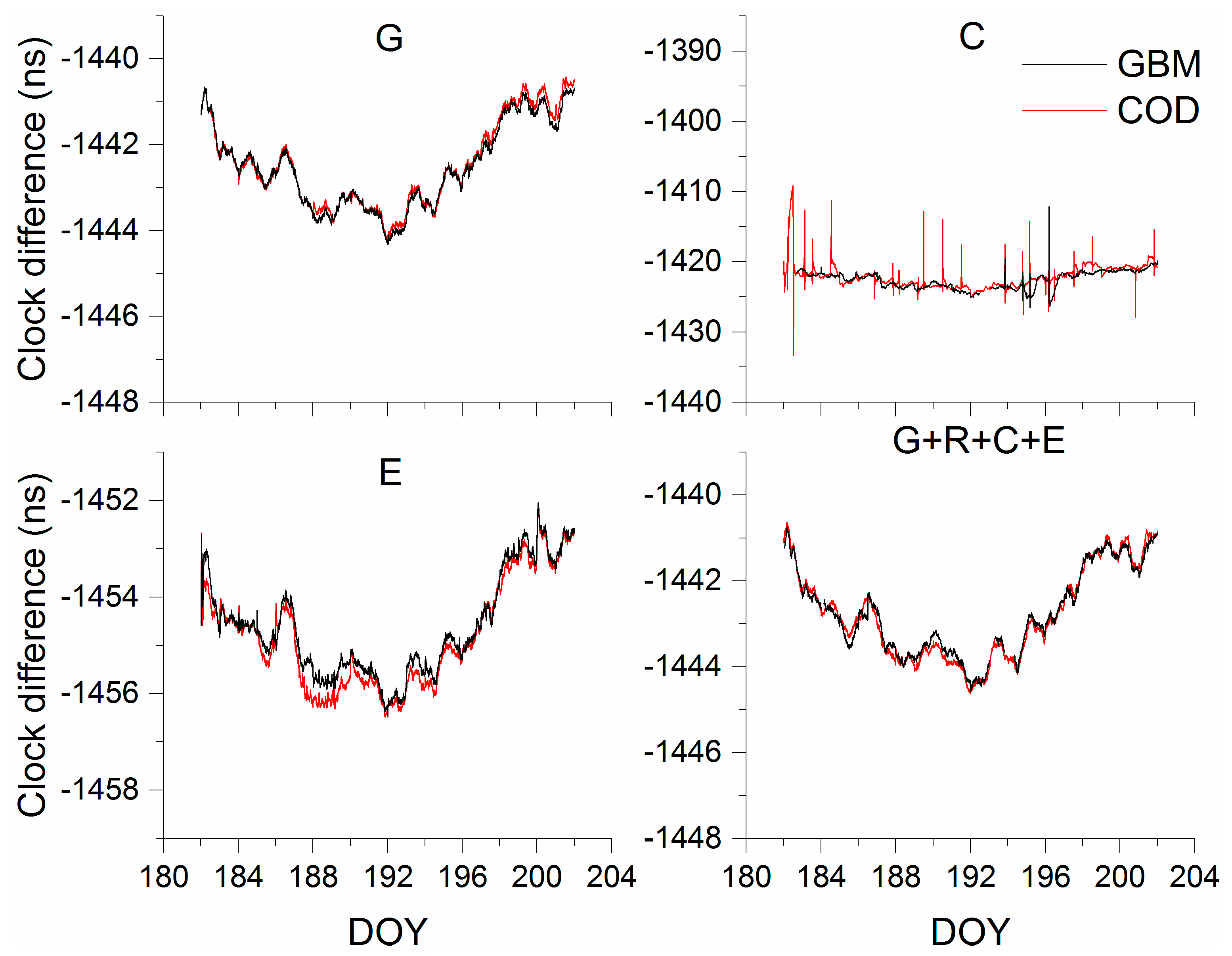
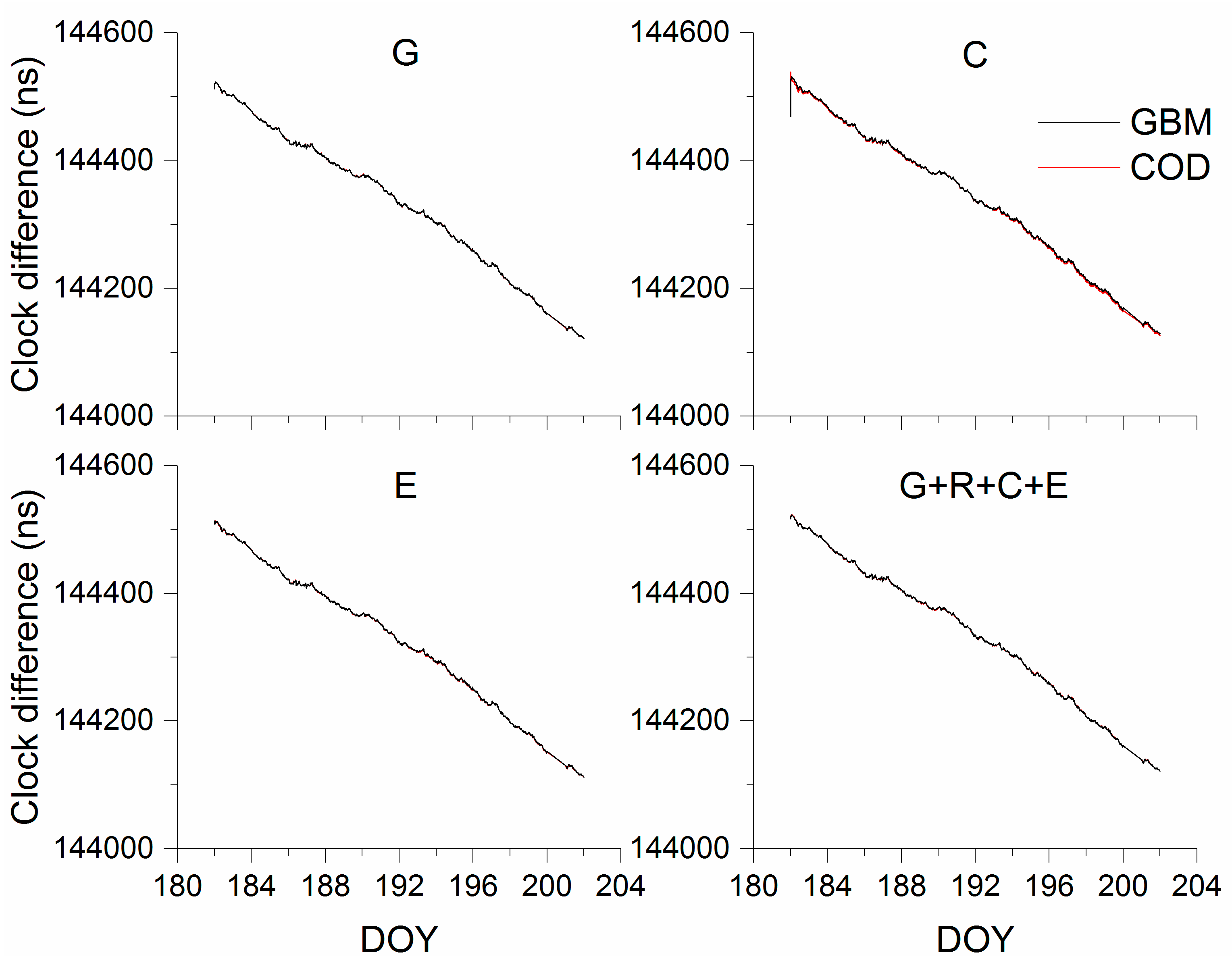
Figure 4 and
Figure 5 depict the clock difference in single-system and multi-GNSS models using GBM and COD products on BRUX-NTSC and HARB-NTSC, respectively. Taken together, we make two remarks here. First, the system bias disappears when using different precise products due to the elimination of the reference time. Second, the variations in GPS-only, Galileo-only, and multi-GNSS PPP time transfer values are in good agreement with each other, while BDS-only performs worse on the BRUX-NTSC time link. Interestingly, the variations in time transfer values are in good agreement with the results for each scheme on the HARB-NTSC time link. The major reason for this may be explained by
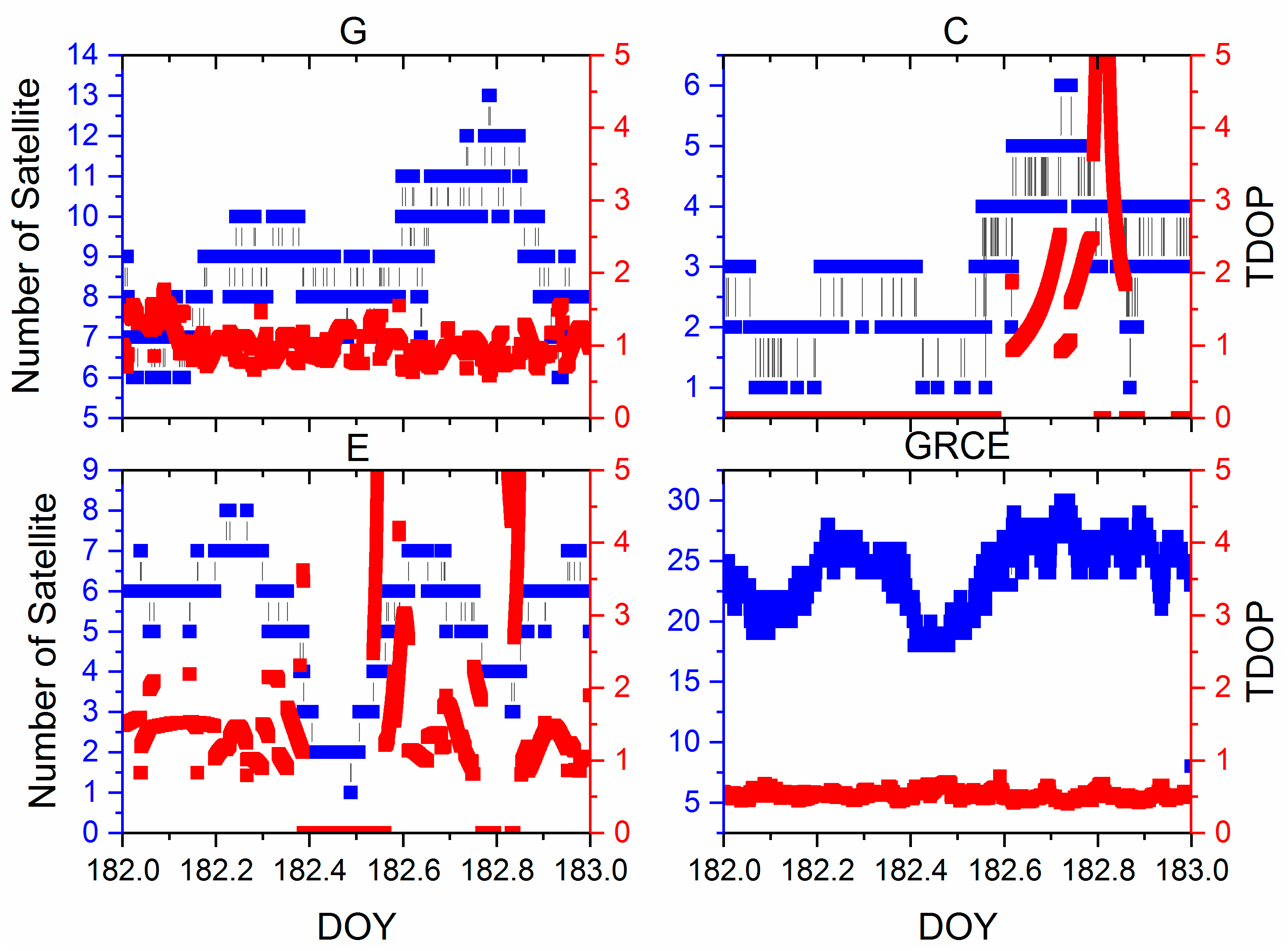
Figure 6 and
Figure 7, depicting the number of satellites and the time dilution of precision (TDOP) for GPS, BDS, Galileo, and multi-GNSS methods at the BRUX and NTSC stations on DOY 182, 2018. For the 10° elevation cut-off, the mean number of satellites is 24.1 for multi-GNSS, 8.8 for GPS, 4.1 for BDS, and 5.2 for Galileo at BRUX. The number of available satellites in the multi-GNSS is more than doubled, as compared with GPS-only. However, this number is the lowest in BDS, which directly affects the accuracy of the results. For the NTSC station, the mean values are increased from 8.2 (GPS-only) to 28.2 (multi-GNSS). More importantly, the mean number of BDS is 9.8. Hence, we can conclude that the number of BDS is analogous to GPS in Asia-Pacific. In addition, the receiver clock offset is of interest in the timing community. The multi-GNSS will improve the accuracy by improving the tracking with a reduction in TDOP. The mean TDOP is 1.2 for GPS, 1.5 for BDS, 2.5 for Galileo, and 0.5 for multi-GNSS at the NTSC station. In addition, the mean TDOP is 1.0 for GPS, 4.2 for BDS, 1.8 for Galileo, and 0.5 for multi-GNSS at BRUX. The TDOP is clearly improved by multi-GNSS, as compared to a single system. Hence, the multi-GNSS solution exhibits improved robustness compared to individual single-system solutions.
To further quantify this agreement, we calculated the root mean square (RMS) value for the smooth result, which is usually employed in the timing community [
23]. Unlike precise positioning, the two external time and frequency references are equipped with two receivers of one time link, which affects the performance evaluation for different time transfer schemes. The vondrak smoothing method [
23] is applied to provide the corresponding RMS values. Time link residuals compared with vondrak smoothing values using COD and GBM products are presented in
Table 3 and
Table 4, respectively. In addition, the improvement of multi-GNSS with respect to GPS-only, BDS-only, and Galileo-only methods is clearly listed. Combining
Table 3 and
Table 4, we have two key findings. First, the performances of time transfer with single-system or multi-GNSS PPP using GBM and COD products are in good agreement with each other. Hence, we can conclude that multi-GNSS PPP transfer with GBM and COD products show the same performance. Second, we can clearly see that multi-GNSS PPP solutions have less noise compared to the single-system solutions, especially with respect to the BDS-only and Galileo-only results at the Eurasia time links, while it is relatively small in the Asia-Pacific time links. For the Eurasia time links, maximum improvements of the multi-GNSS solutions are up to 18.2%, 96.6%, and 53.7% compared to the GPS-only, BDS-only, and Galileo-only solutions, respectively, using COD products. With respect to the Asia-Pacific time links, the maximum improvements of the multi-GNSS solutions are up to 3.5%, 31.1%, and 6.5% compared to the GPS-only, BDS-only and Galileo-only solutions, respectively. For single-system and multi-GNSS PPP with GBM products, maximum improvements of multi-GNSS solutions are up to 7.4%, 94.0%, and 57.3% compared to the GPS-only, BDS-only and Galileo-only solutions, respectively, for all results.
In
Table 3 and
Table 4, (%) indicates the improvement of multi-GNSS with respect to the GPS-only, BDS-only and Galileo-only solutions.
The time link is equipped with two different time and frequency references. Therefore, it is complicated to evaluate the performance of the PPP time transfer due to the absence of an absolute standard for comparison. Hence, the Allan deviation (ADEV) was applied to obtain the frequency stability [
12,
15] and to further assess the performance of the single-system and multi-GNSS solutions.
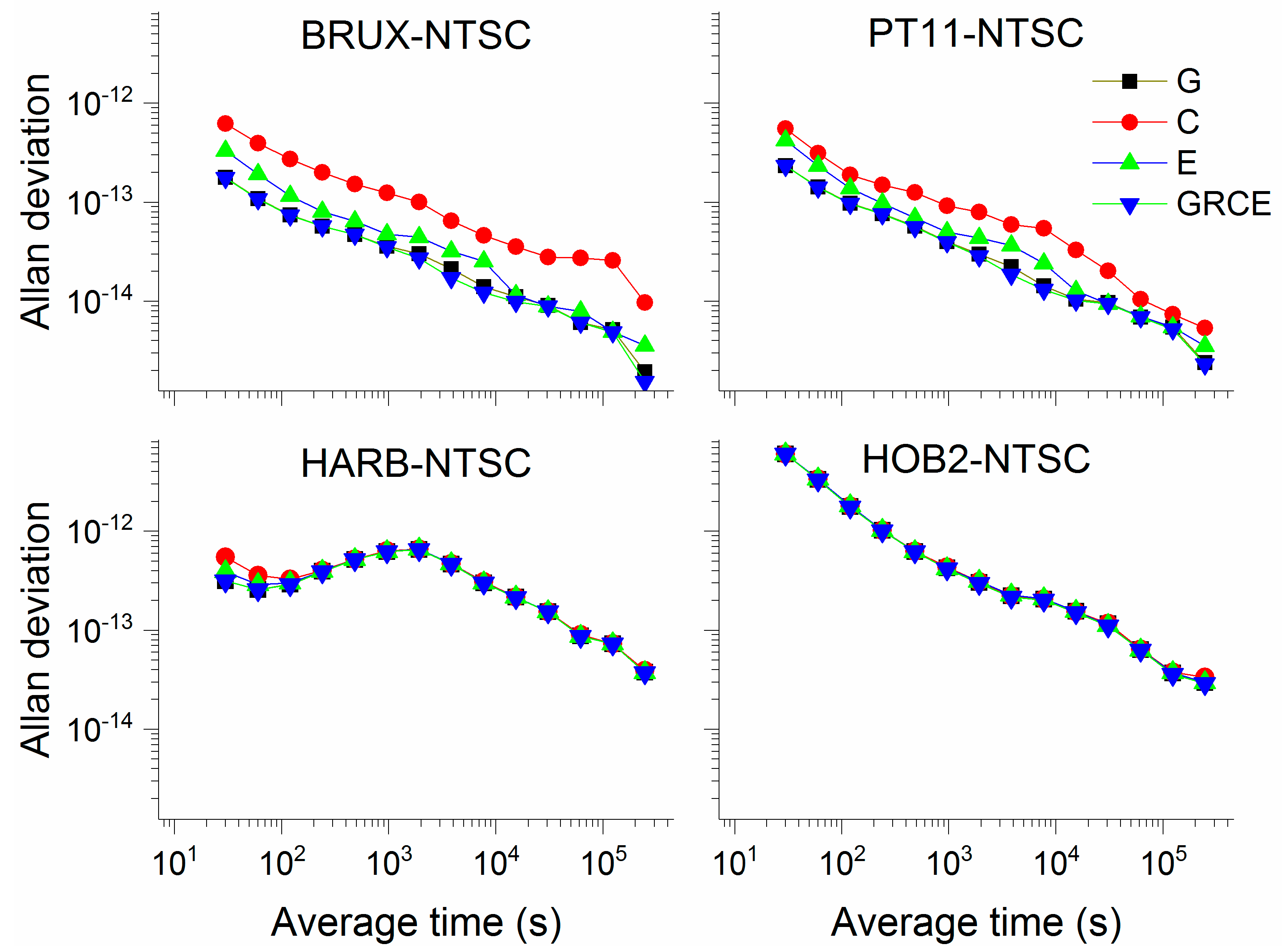
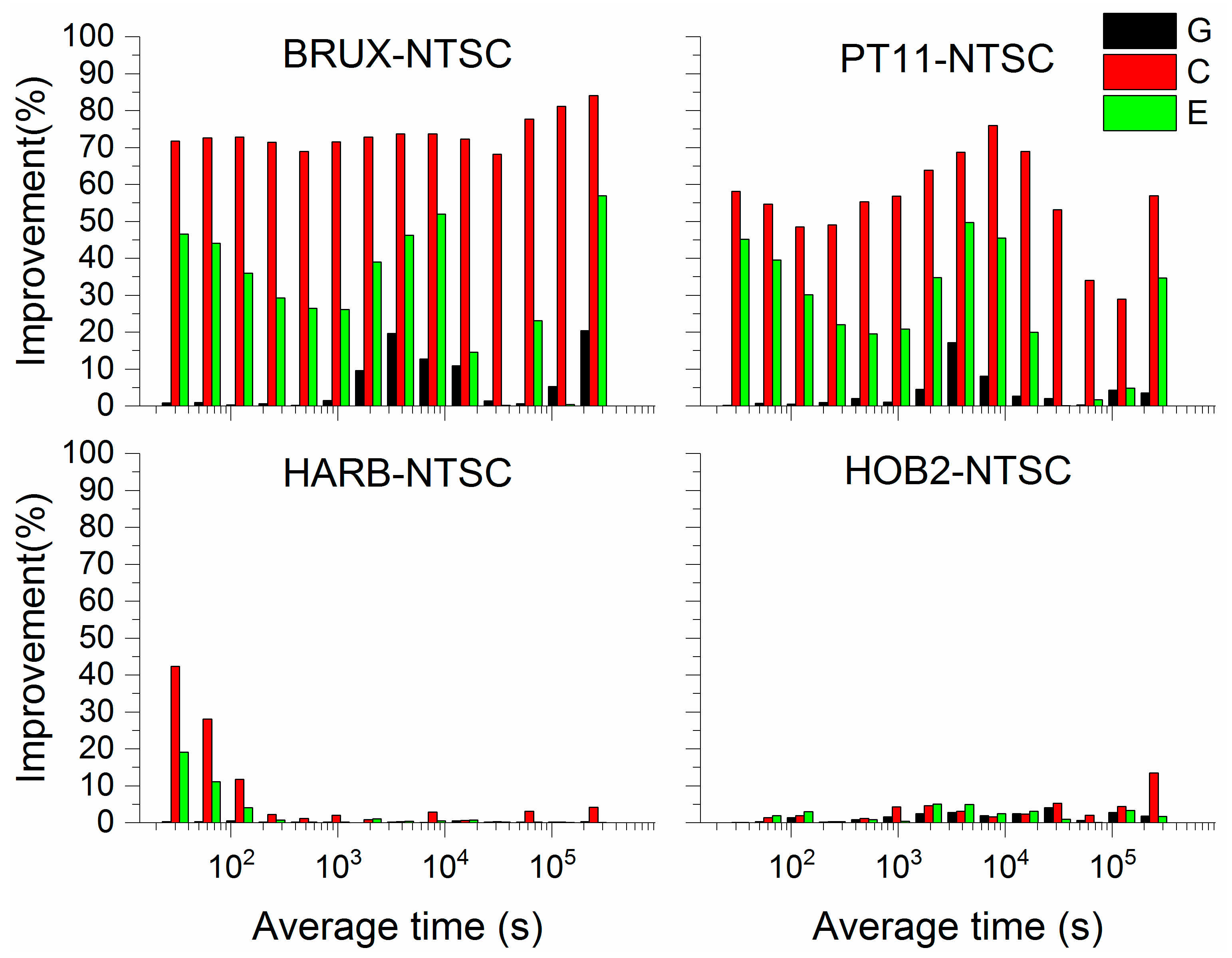
Figure 8 presents the frequency stability of the single-system and multi-GNSS solutions for four time links using COD products. In addition, the percentage improvement of multi-GNSS stability over individual systems is displayed in
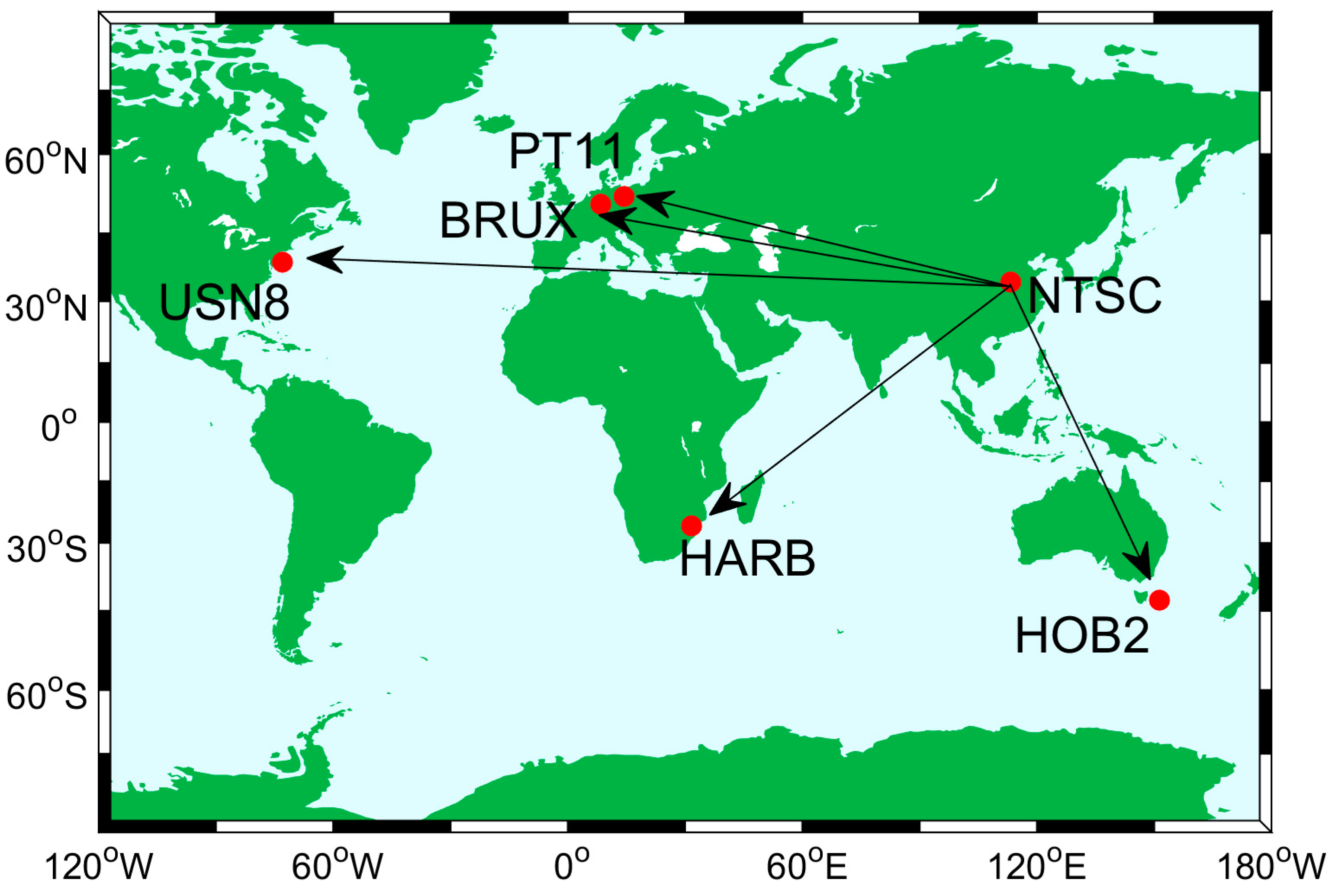
Figure 9 for different average times. Taken together, we obtain three findings here. First, the stability of BRUX-NTSC and PT11-NTSC is better than that of HARB-NTSC and HOB2-NTSC, as evidenced by the fact that the stability of time links is determined by the performance of atomic clocks. We also see that atomic clocks with different performances are equipped at different stations in
Table 1. In addition, NTSC, PT11, and BRUX are located in timing laboratories. Second, the performance of GPS PPP is better than Galileo- and BDS-only PPP solutions in the Eurasia time links [
10] and is similar to those in Asia-Pacific time links. This further validates our previous conclusions. Third, the improvement in the multi-GNSS ranges from 0.1 to 20.3% compared to the GPS-only solution. The multi-GNSS presents a significant improvement over the BDS-only solution in the Eurasia time links. The maximum improvement is up to 84%. For the Galileo-only solution, the improvement ranges from 0.1 to 45.4%.
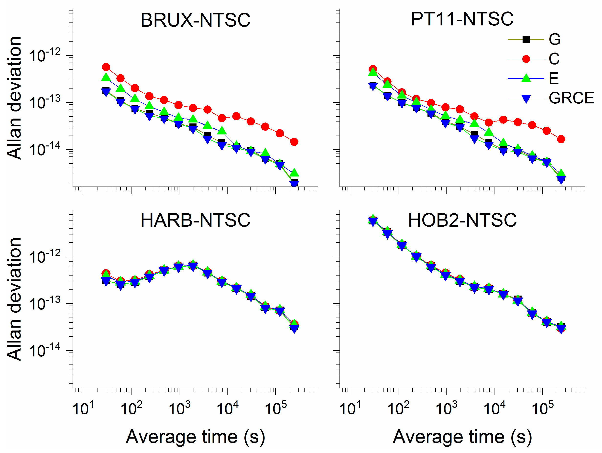
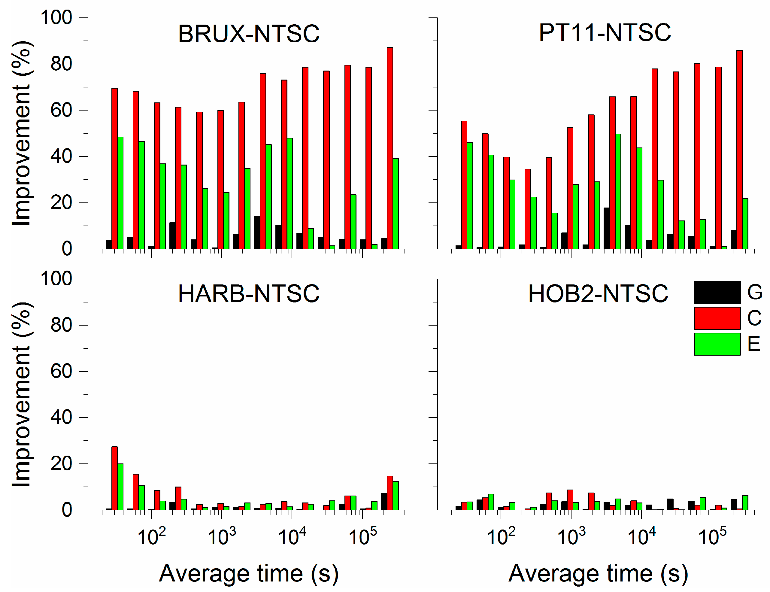
Figure 10 depicts the frequency stability of single-system and multi-GNSS solutions for four time links using GBM products. The percentage improvement of multi-GNSS stability over individual systems is displayed in
Figure 11 for different average times. The results using GBM products are analogous to those using COD products. The improvement in the multi-GNSS ranges from 0.04 to 17.4% compared to the GPS-only solution at different average times. The multi-GNSS presents a significant improvement over the BDS-only solution in the Eurasia time links. The maximum improvement is up to 87.2%. For the Galileo-only solution, the improvement ranges from 1.1 to 49.2%, the averages are 27.3%, 30.1%, 5.6%, and 3.4% for PT11-NTSC, BRUX-NTSC, HOB2-NTSC, and HARB-NTSC, respectively.
4.2. Multi-GNSS PPP Time Transfer with the Between-Epoch Constraint Model
In this subsection, based on the multi-GNSS PPP method and the between-epoch constraint model, two schemes were designed. For convenience, the two schemes summarized in
Table 5 are marked as scheme1 and scheme2.
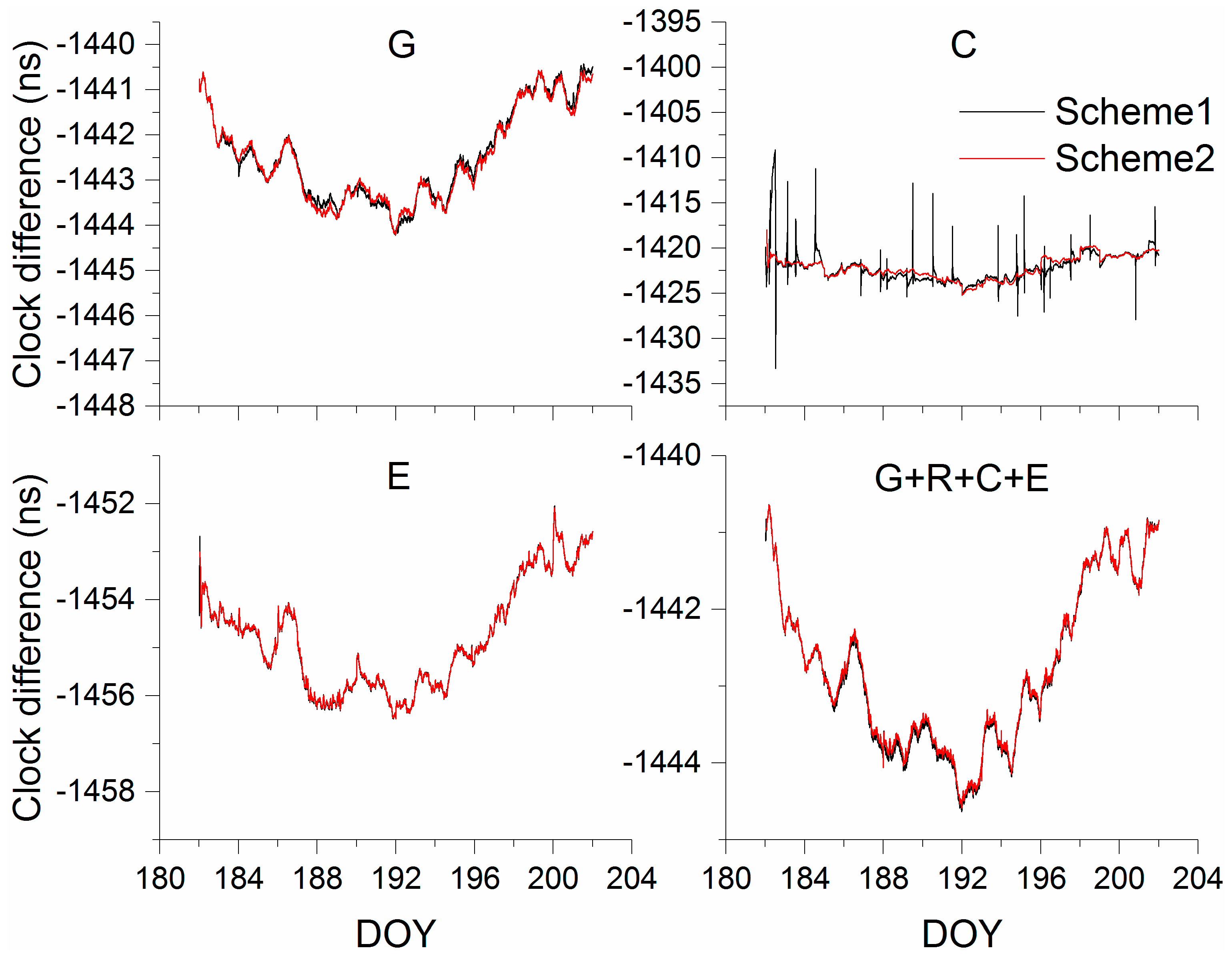
Figure 12 and
Figure 13 show the clock difference of scheme1 and scheme2 with single-system and multi-GNSS models on BRUX-NTSC and HARB-NTSC, respectively, using COD products. Combining
Figure 12 and
Figure 13, two findings are marked here. First, scheme1 and scheme2 have no system bias and have good consistency, which illustrates the feasibility of our model. Second, interestingly, our method can significantly improve the performance of BDS PPP in the Eurasia link because the receiver in the European region observed a relatively small number of BDS satellites, and the geometry strength is not very high. The between-epoch constraint model was employed to estimate the clock offset in scheme2, which will improve the strength of the equation. In addition, some BDS satellites have lower elevation angles in the European region. The between-epoch constraint model reduces the amount of noise absorbed by the receiver clock offset and improves the accuracy of BDS PPP time transfer.
In order to analyze the two schemes, we used the results of vondrak smoothing as a reference. The RMS values of the difference between the two schemes and the smoothing results were obtained. Results are presented in
Table 6 and
Table 7. The main conclusion to be drawn from
Figure 12 and
Figure 13, in conjunction with
Table 6 and
Table 7, is straightforward. It is clear that scheme2 contains less noise compared to scheme1, whether a single-system model or a multi-GNSS model is used. The improvement of scheme2 ranges from 36.5 to 92.2% compared with scheme1 for the GPS-only solution. Compared to scheme1, the solutions of scheme2 are improved by 11.8–39.3%, 6.6–43.3%, and 15.0–90.9% for BDS-only, Galileo-only, and multi-GNSS solutions. More interestingly, the performance of scheme2 using GBM products is similar to that using COD products. This can explain that our approach is suitable for different products. The solutions of scheme2 are improved by 37.8–91.9%, 10.5–65.8%, 2.7–43.1%, and 26.6–86.0% using the GPS-only, BDS-only, Galileo-only, and multi-GNSS solutions.
In
Table 6 and
Table 7, 1 and 2 represent scheme1 and scheme2, respectively. (%) is the improvement of scheme2 compared to scheme1.
As mentioned previously, an absolute standard for comparison is lacking. Here, ADEV is considered again to further assess how well our approach performs for multi-GNSS PPP time and frequency transfer.
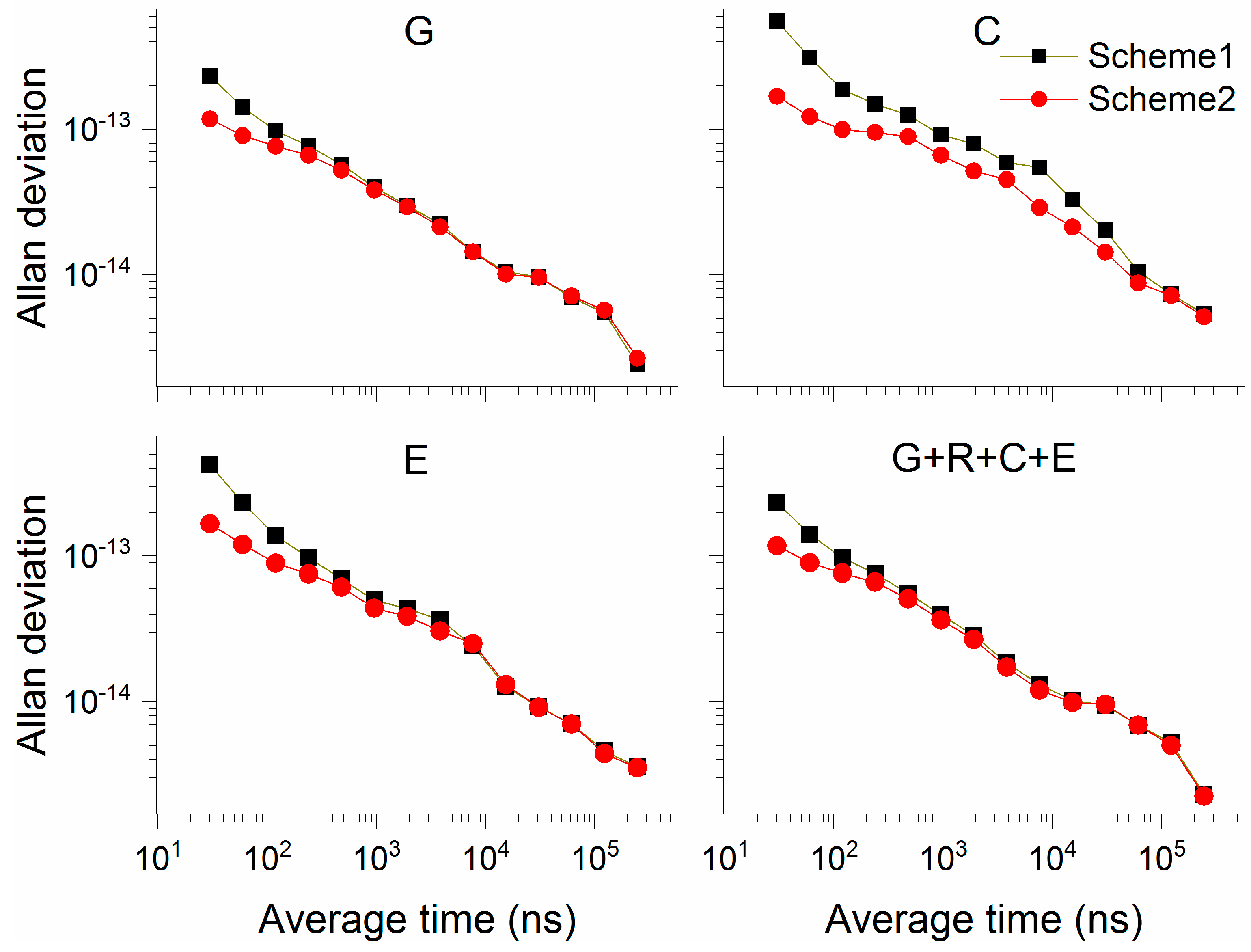
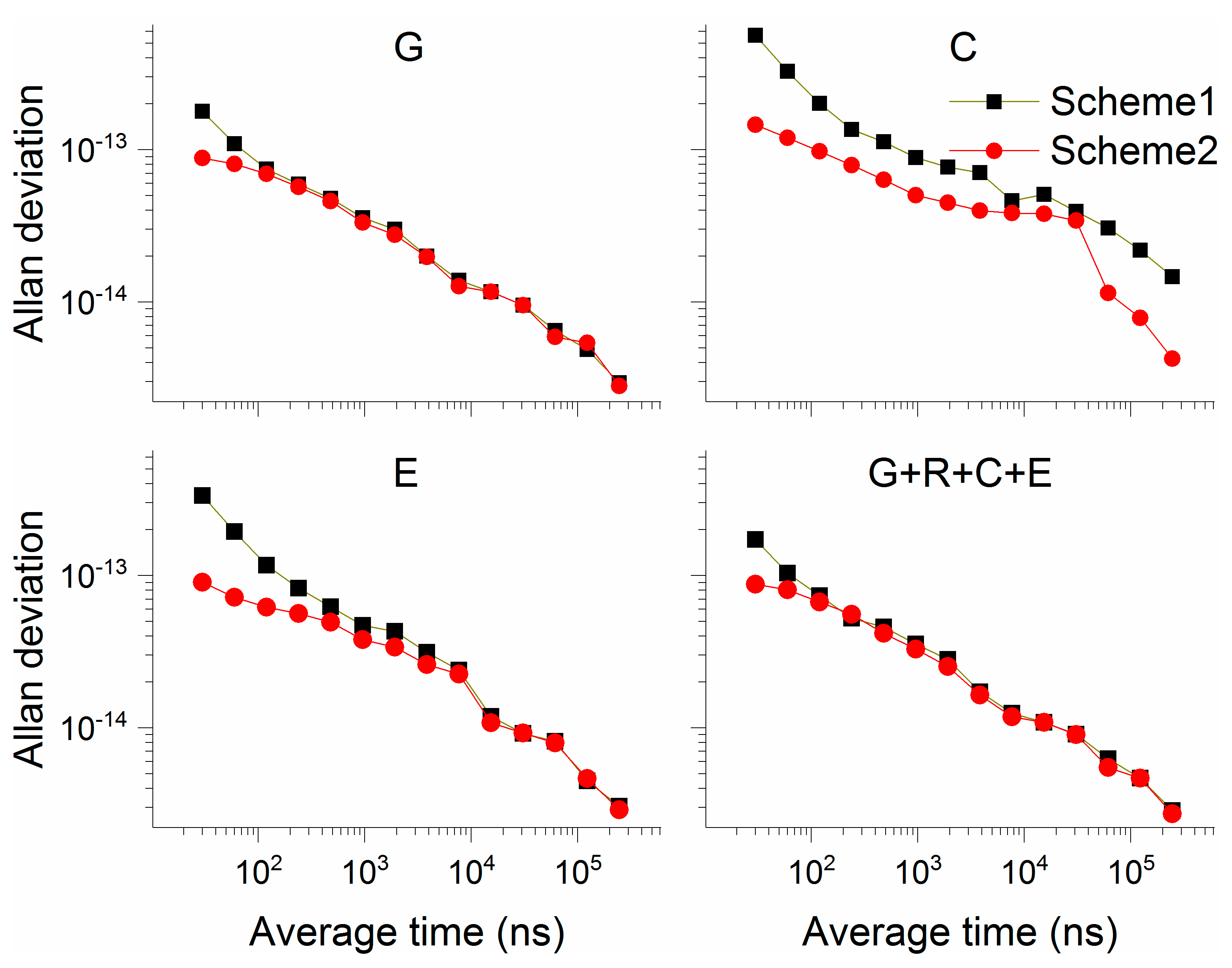
Figure 14 and
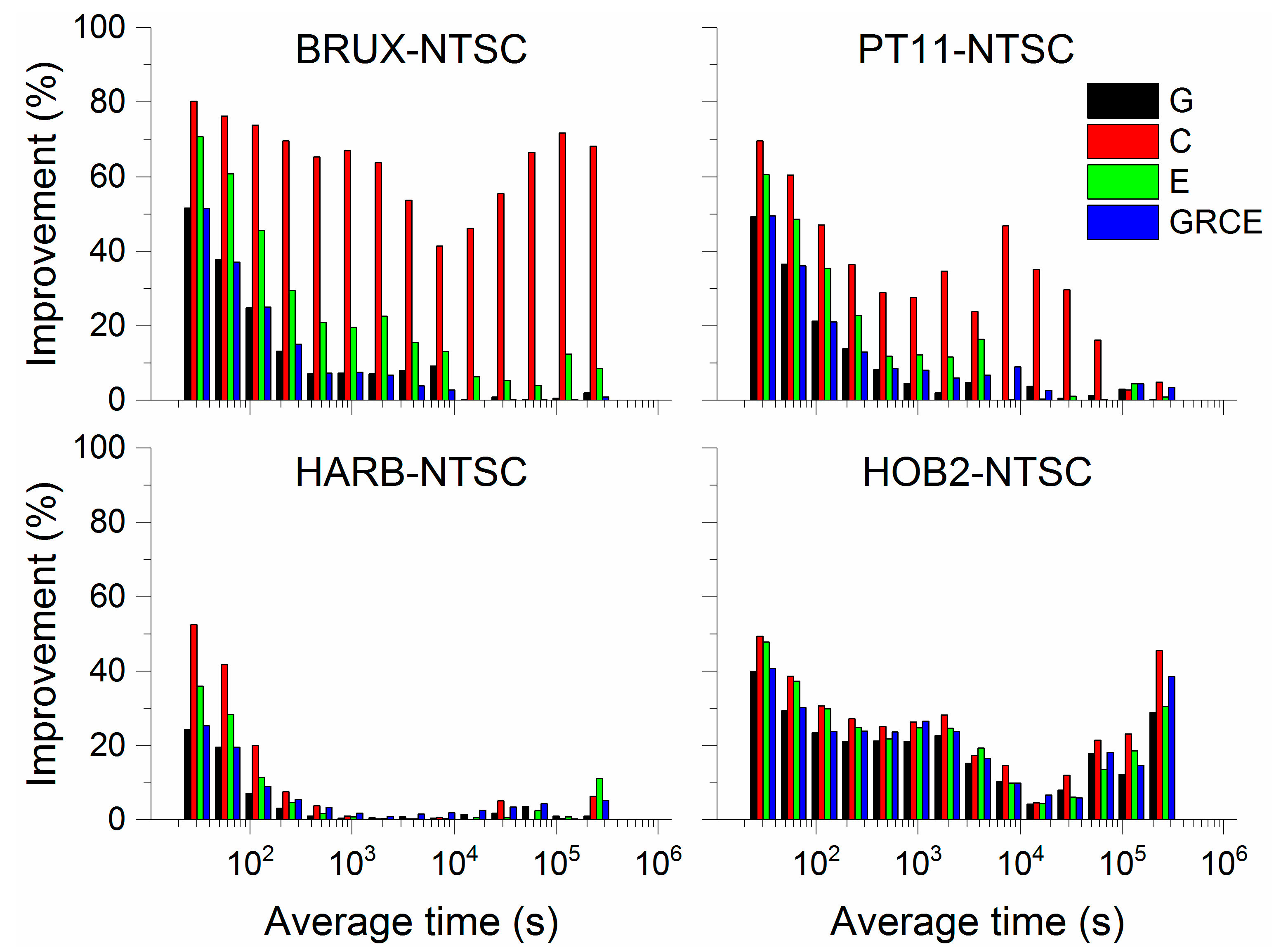
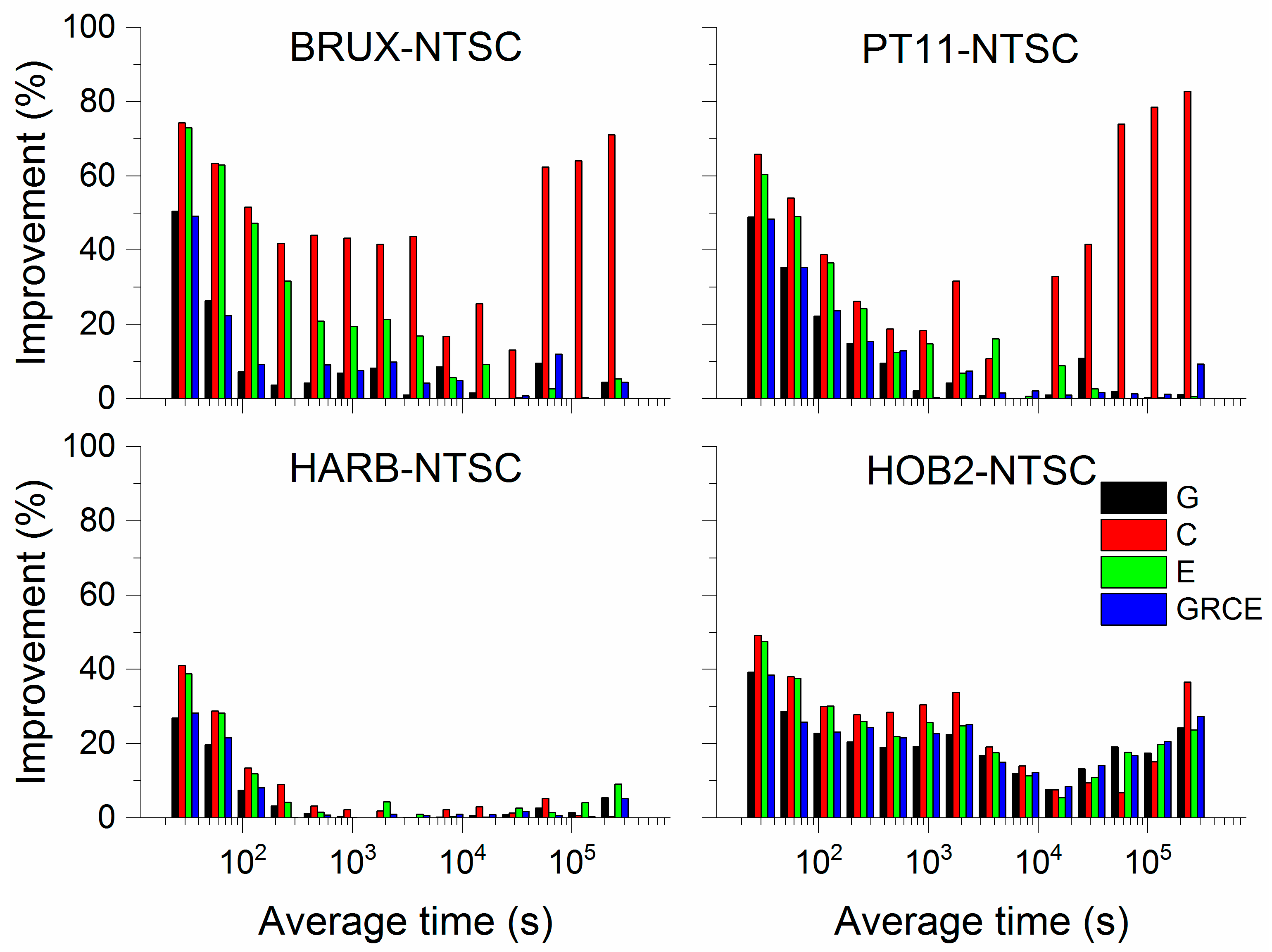
Figure 15 show the Allan deviation of scheme1 and scheme2 on PT11-NTSC and HOB2-NTSC, respectively, with single-system and multi-GNSS models using COD products. Overall, the results show that in each panel the frequency stability is notably improved, especially for short-term stability, and that, in accordance with our expectation, each result using single-system or multi-GNSS models exhibits different degrees of improvement. We surmise that this may be because, applying our approach, the noise of the clock offset is reduced significantly. To further quantify this improvement, the improvement of the four time links was calculated, and the results are displayed in
Figure 16. A significant improvement is clear in the Eurasia links, especially for the BDS-only and Galileo-only models. This further explains that our approach performs better than scheme1, especially for the few observed satellites. For the Eurasia links, the improvement of scheme2 ranges from 0.2 to 51.6%, from 3 to 80.0%, from 0.2 to 70.8%, and from 0.1 to 51.5% for the GPS-only, BDS-only, Galileo-only and multi-GNSS PPP solutions compared to scheme1. In addition, the performances of scheme2 are improved by 0.3–39.9%, 0.1–52.5%, 0.2–47.8%, and 0.1–40.7% for GPS-only, BDS-only, Galileo-only, and multi-GNSS PPP solutions compared to scheme1 in Asia-Pacific.
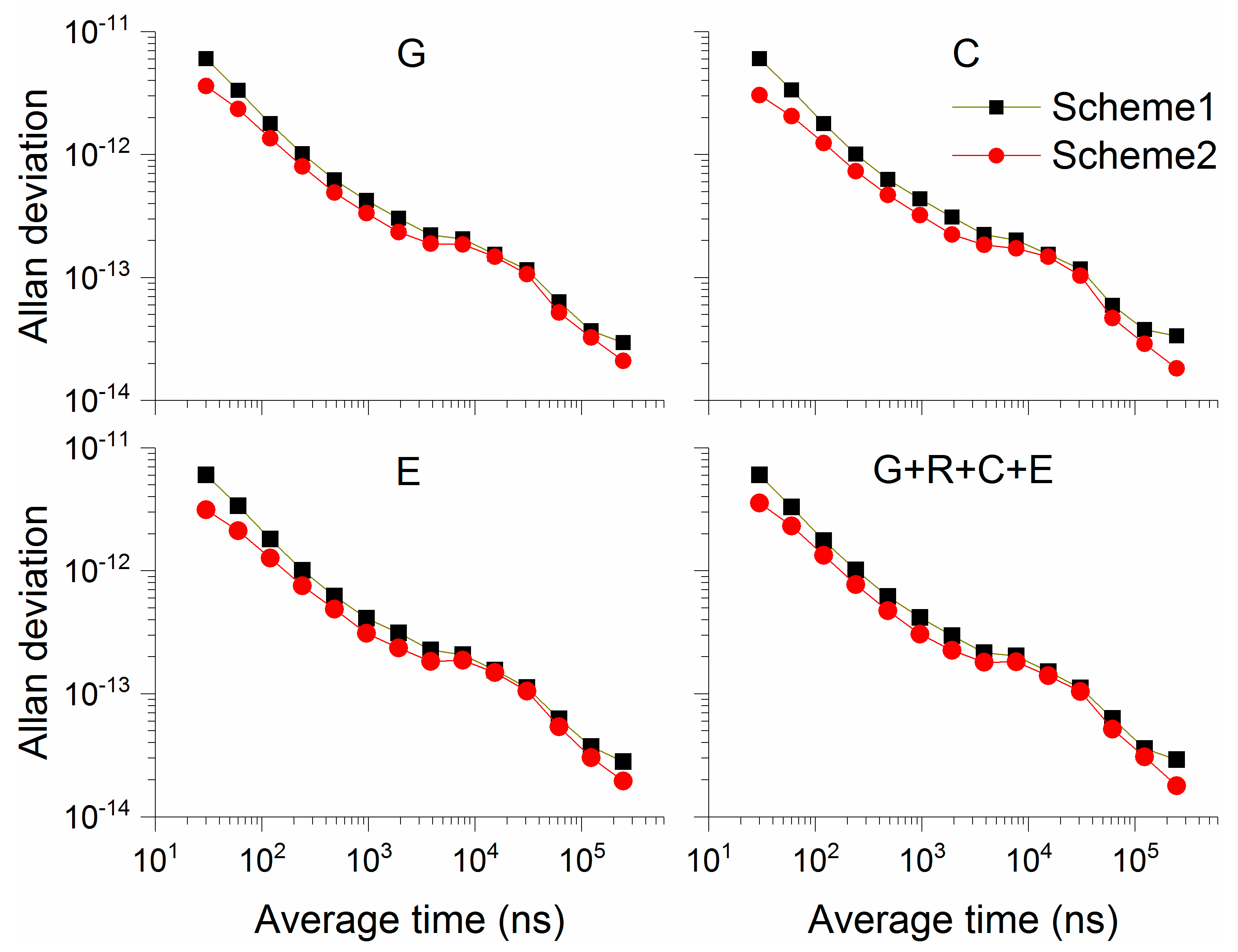
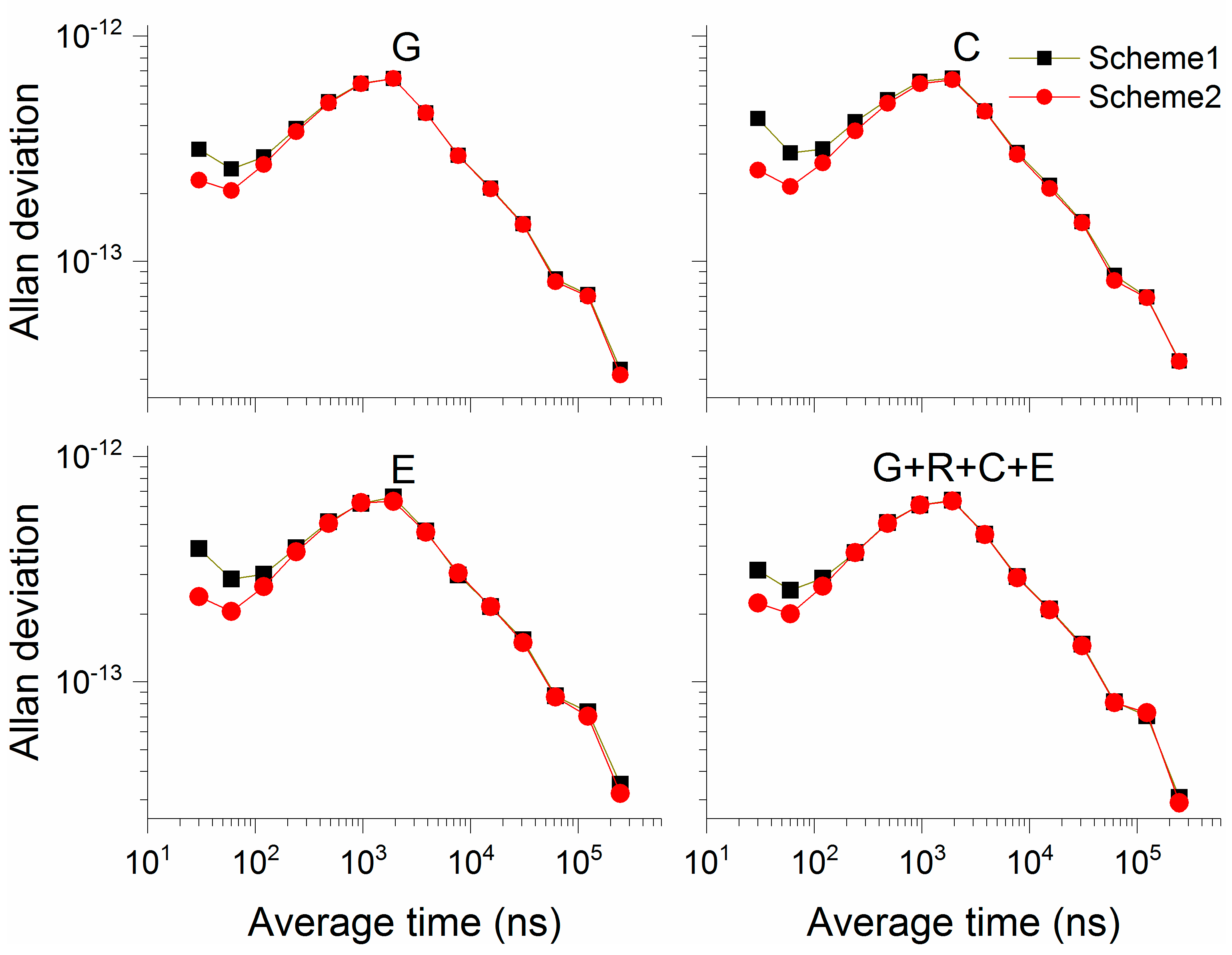
Figure 17 and
Figure 18 show Allan deviation of scheme1 and scheme2 on BRUX-NTSC and HARB-NTSC, respectively, with single-system and multi-GNSS models using GBM products. Like the solutions using COD products, it follows that, in each panel, the frequency stability is significantly improved, especially for short-term stability. The improvement of the four time links was calculated, and the results are displayed in
Figure 19. For the Eurasia links, the improvement of scheme2 ranges from 0.1 to 50.4%, from 0.1 to 74.2%, from 0.2 to 72.9%, and from 0.9 to 49.1% for GPS-only, BDS-only, Galileo-only, and multi-GNSS PPP solutions compared to scheme1. In addition, the performances of scheme2 are improved by 0.3–39.2%, 0.4–41.0%, 0.2–47.4%, and 0.1–38.4% for GPS-only, BDS-only, Galileo-only, and multi-GNSS PPP solutions compared to scheme1.

 ,
, 


