New Approaches for Robust and Efficient Detection of Persistent Scatterers in SAR Tomography

1
College of Electronic Science, National University of Defense Technology, No. 109 De Ya Road, Changsha 410073, China
2
China Electronic Technology Group Corporation (CETC), Wan Shou Road, Beijing 100000, China
*
Author to whom correspondence should be addressed.
Remote Sens. 2019, 11(3), 356; https://0-doi-org.brum.beds.ac.uk/10.3390/rs11030356
Submission received: 3 January 2019
/
Revised: 3 February 2019
/
Accepted: 3 February 2019
/
Published: 11 February 2019
Abstract
:Persistent scatterer interferometry (PSI) has the ability to acquire submeter-scale digital elevation model (DEM) and millimeter-scale deformation. A limitation to the application of PSI is that only single persistent scatterers (SPSs) are detected, and pixels with multiple dominant scatterers from different sources are discarded in PSI processing. Synthetic aperture radar (SAR) tomography is a promising technique capable of resolving layovers. In this paper, new approaches based on a novel two-tier network aimed at robust and efficient detection of persistent scatterers (PSs) are presented. The calibration of atmospheric phase screen (APS) and the detection of PSs can be jointly implemented in the novel two-tier network. A residue-to-signal ratio (RSR) estimator is proposed to evaluate whether the APS is effectively calibrated and to select reliable PSs with accurate estimation. In the first-tier network, a Delaunay triangulation network is constructed for APS calibration and SPS detection. RSR thresholding is used to adjust the first-tier network by discarding arcs and SPS candidates (SPSCs) with inaccurate estimation, yielding more than one main network in the first-tier network. After network adjustment, we attempt to establish reliable SPS arcs to connect the main isolated networks, and the expanded largest connected network is then formed with more manual structure information subtracted. Furthermore, rather than the weighted least square (WLS) estimator, a network decomposition WLS (ND-WLS) estimator is proposed to accelerate the retrieval of absolute parameters from the expanded largest connected network, which is quite useful for large network inversion. In the second-tier network, the remaining SPSs and all the double PSs (DPSs) are detected and estimated with reference to the expanded largest connected network. Compared with traditional two-tier network-based methods, more PSs can be robustly and efficiently detected by the proposed new approaches. Experiments on interferometric high resolution TerraSAR-X SAR images are given to demonstrate the merits of the new approaches.
1. Introduction
Persistent scatterer interferometry (PSI), an advanced remote sensing technique, has been widely applied in long-term deformation monitoring [1,2,3,4,5] in urban areas using time-coherent pixels. However, an inherent limitation of PSI is that a persistent scatterer (PS) is assumed to be a single dominant scatterer within a pixel. This assumption may not be correct in real environments, especially in urban areas with many high-rise buildings. As a result, pixels with multiple dominant scatterers cannot be detected, and this may cause incorrect parameter estimation.
Synthetic aperture radar (SAR) tomography is a powerful remote sensing technique, which allows SAR imaging to be extended to three-dimensional (3-D) imaging of volumetric targets using several images of a scene acquired with different viewing angles [6,7,8,9,10]. This gives it the ability to separate multiple dominant scatterers in a resolution cell. Both PSI and SAR tomography detect and estimate time-coherent scatterers from interferometric data stack. The major difference between PSI and SAR tomography is the number of scatterers that are assumed within a resolution cell. Nowadays, modern spaceborne SAR sensors, such as TerraSAR-X [11] and Cosmo-Skymed [12], can provide SAR data with very high resolution of more than one meter. This high resolution offers new opportunities for tomographic mapping of urban areas, even single-built structures.
With reference to the application [13,14,15,16] of SAR tomography, the problem of detecting PSs has become a key issue, receiving much attention in the recent literature. The main interest is concentrated on increasing the number of monitored PSs and keeping low probability of false alarms at the same time. For the detection of PSs, one approach is based on multi-interferogram complex coherence (MICC), which uses phase-matching between the measured signal at different acquisitions and the estimated ideal response, as manifested in [17,18]. Another approach is based on the generalized likelihood ratio test (GLRT) [19,20], which exploits both the amplitude and phase information. The GLRT outperforms the MICC, which uses only the phase information. The superior performances are measured as an increase in the detection probability for a fixed false alarm level as well as an increase in the accuracy of parameter estimation. Both approaches are based on the assumption that the atmospheric phase screen (APS) has been separated from the acquisitions, at least on a small scale, before the detection of PSs.
However, real acquisitions do not satisfy this assumption. For repeat-pass SAR systems, the interferometric stack of complex-valued SAR images with diversity in space and time is inevitably affected by the temporally uncorrelated APS, which significantly degrades the quality of tomographic inversion in cross-slant range direction, resulting in high sidelobe and even defocusing. Consequently, large-scale APS has a big impact on the detection and estimation of PSs, so we consider APS calibration as the prerequisite of PS detection. Prior to the PS detection, the APS must be calibrated from SAR acquisitions.
To our knowledge, the atmosphere can be divided into many different layers, and the two major layers of the atmosphere are troposphere and ionosphere. Previous studies have shown that water vapor and clouds present in the troposphere and the total electron content (TEC) in the ionosphere are responsible for APS. As for APS calibration, plentiful research has been done and different methods have been proposed over time, which can be mainly divided into three categories.
First, the APS can be calculated and removed with external measurement data. In [21], the Moderate Resolution Imaging Spectroradiometer (MODIS) [22] data and global ionospheric maps (GIMs) [23,24] were utilized to calculate and subtract the tropospheric and ionospheric phase screen, respectively. MODIS is a spectrometer that provides products with three different spatial resolutions: 250 m, 500 m, and 1000 m. The GIMs are generated from GPS-tracking data with an accuracy of approximately 0.8 TECU on a daily basis (1 TEC unit is equivalent to a TEC of ). Due to the sparse grid of external measurement data, this approach for APS calibration has low precision. Second, the APS can be filtered out as the APS is spatially low frequency and temporally high frequency. In [8,25,26,27], spatiotemporal filtering method was presented for large-scale APS calibration, which is extensively employed in PSI. This method relies on the setting of the filtering parameter. Both under-filtering and over-filtering will result in inaccurate APS subtraction. In practice, the adjustment of the filtering parameter should be decided according to the experimental area. Third, the APS of the image pixels near the reference PS can be directly removed by subtracting the phase of the reference PS. This method takes advantage of the characteristic that the APS is spatially low frequency. In this way, the APS can be calibrated to a small scale with no need to estimate it by constructing a reference network, as shown in [28]. After APS calibration, it is possible that PSs can be properly detected and estimated. Based on this principle, a SAR-tomography-based persistent scatterer interferometry (Tomo-PSInSAR) method, implemented upon a traditional two-tier network, can be used for robust detection of PSs, as shown in [29]. In the first-tier network, a Delaunay triangulation network is constructed, and the APS is calibrated. Then, the detection and the relative estimation of SPS pairs are performed. After network adjustment, there is high probability that some main isolated networks yield in the first-tier network, and the largest one is utilized to retrieve the absolute estimation by the weighted least square (WLS) [29,30,31] estimator. In the second-tier network, arcs with SPSs of the largest connected network in the first-tier network as reference points are constructed, and the APS is calibrated by subtracting the phase of reference SPSs. Then, the remaining SPSs and all the DPSs can be detected. The distribution of the largest connected network utilized in the first-tier network determines the amount of manual structure information available through the two-tier network. The traditional two-tier network can be well applied for the detection of PSs.
However, there are two problems with the traditional two-tier network. Firstly, it is not appropriate to merely utilize the largest connected network in the first-tier network and omit other smaller ones because all of the main isolated networks in the first-tier network carry much useful structure information of the observed scene. The manual structure information of the area covered by the other main networks cannot be acquired by merely utilizing the largest network. Secondly, there is a huge computation burden if we directly apply WLS estimator for retrieving the absolute parameters in the whole area, especially for large network inversion.
In this context, new approaches based on a novel two-tier network are proposed in this paper. In the first-tier network, we attempt to establish reliable arcs among the main isolated networks. As a result, the largest connected network is expanded with more manual structure information subtracted. In order to measure whether the APS is effectively calibrated and to select PSs with accurate estimation, a residue-to-signal ratio (RSR) estimator is proposed. In addition, we provide a network decomposition WLS (ND-WLS) estimator to improve the efficiency of the integration process with accuracy maintenance. Through the new approaches, more SPS and DPSs with more manual structure information can be robustly and efficiently detected.
The rest of the paper is structured as follows. In Section 2, the signal model of three-dimensional SAR tomography and new approaches for robust and efficient detection of PSs are introduced. Therein, the RSR estimator and ND-WLS estimator are provided. Section 3 presents the results of TerraSAR-X in an urban area using the proposed new approaches. Conclusions and future work are presented in Section 4.
2. Basic Theory and New Approaches for the Detection of PSs
2.1. Signal Model of Three-Dimensional SAR Tomography
For the measurement of an azimuth-range pixel exhibiting point scattering information from one or more targets, SAR tomography without error can be modeled as follows [32,33,34]:
where is the reflectivity function of slant elevation , and denotes the extension of . The phase item that simultaneously models the phase component at elevation can be written as follows:
where is the spatial frequency, with denoting the perpendicular component of spatial baseline of measurement (respect to the master measurement), denoting the slant range, and denoting the wave length of the SAR system.
For repeat-pass spaceborne SAR systems, APS and noise always exists in real measurements, as depicted in Figure 1. Then, Equations (1) and (2) can be recast as follows:
where is the noise accounting for thermal noise and baseline decorrelation, which has a strong impact on low backscatter pixels; otherwise, the influence of on the strong backscatter pixels can be neglected. is the phase contribution of APS.
When APS is removed, Equation (3) can also be written as follows:
where is the measurement vector ( represents the transpose operation), is the system matrix with , is the reflectivity vector to be estimated, and is the noise vector.
2.2. New Approaches for the Detection of PSs
In this section, new approaches based on a novel two-tier network aimed at APS calibration and robust and efficient PS detection is introduced. The novel two-tier network can be divided into three steps: first-tier network construction and APS calibration, largest connected network establishment and ND-WLS estimation, second-tier network construction and detection of the remaining PSs. In the first-tier network, a Delaunay triangulation network is constructed, and the APS is calibrated. After removing the APS, SPSs are detected, and relative estimates can be acquired. To measure whether the APS is effectively calibrated and to select reliable PSs with accurate estimation, a RSR estimator is introduced. Thereafter, reliable arcs are established to connect the main isolated networks, and the expanded largest connected network is then established. Afterward, the ND-WLS estimator is employed to retrieve absolute estimates from the expanded largest connected network with more efficiency. In the second-tier network, the remaining reliable SPSs and all the DPSs are detected with reference to the expanded largest connected network. The flowchart of the proposed new approaches is depicted in Figure 2.
2.2.1. First-Tier Network Construction and APS Calibration
First, initial selection of the potential SPSs is performed. In this paper, amplitude dispersion [20,35] is employed for the primary selection of SPS candidates (SPSCs) with high amplitude stability and high signal-to-noise ratio (SNR). Then, the SPSCs are connected by constructing a Delaunay triangulation network, which is regarded as the first-tier network.
For a pair of connected SPSCs of one arc in the first-tier network, the real measured tomographic signals and of two SPSCs can be modeled as follows:
where and represent the APS existing in and , respectively; and are the slant elevation of the two connected SPSCs, respectively; and and denote the ideal measurement of the two SPSCs without APS interference.
Because the APS is temporally uncorrelated, it will seriously destroy the phase information of ideal tomographic signal if not calibrated. Therefore, APS calibration is considered to be the prerequisite for the detection and estimation of PSs. In view of the fact that the APS is spatially low frequency, SPSCs with long spatial distance normally have a big difference in APS. Typically, it is difficult to cope with the connected SPSCs with a big APS difference. Thus, distance threshold is used to first reject the long arcs. When the arc is of short distance, there is high probability that the two adjacent SPSCs have similar APS:
Thus, it is easy to calibrate the APS by subtracting the phase of the reference point, and the relative tomographic signal of the arc can be given as follows:
where is the phase-preserving operation.
After removing the APS for all arcs, it is possible to properly determine whether the SPSCs in the first-tier network are true SPSs. Different strategies have been proposed over time for the detection and estimation of PSs, as in [7,36,37,38] and [19,20,39,40]. It was shown in [20] that the sequential generalized likelihood ratio test with cancellation (SGLRTC) has a good performance, both in terms of high detection probability for a given level of false alarm as well as high accuracy. Beam-Forming (BF) as a nonparametric method has been widely applied owing to its high efficiency and robustness. The resolution and sidelobe of the BF method is determined by the extension and distribution of baselines. In this paper, we use BF as the merit function for tomographic inversion associated with SGLRTC as a PS detection strategy. If the two connected SPSCs are true SPSs, Equation (7) can be rewritten as follows:
where defines the amplitude-preserving operation. The relative tomographic signal of the arc with two connected true SPSs can be detected like a true SPS. We define this kind of arc as the SPS arc. Therefore, if the relative tomographic signal can be detected like a true SPS by BF-based SGLRTC, we consider the two connected SPSCs at the arc as true SPSs and preserve the SPS arc. Meanwhile, we can acquire the relative elevation.
To measure whether the APS is effectively calibrated and to evaluate the quality of the relative estimates for all arcs, we define RSR estimator, which can be given by the following equation:
where represents the estimated response of the relative tomographic signal by BF-based SGLRTC.
The RSR can serve as a metric for the matching degree between the measurements and the estimated response. Lower RSR value implies a better match. If APS is not effectively calibrated to a small scale, the PSs will not be properly detected and estimated, so the RSR value will be large. Therefore, the RSR can be computed to jointly measure the level of residual APS and evaluate the goodness of estimates. In this paper, we use RSR threshold (typically 0.3) to adjust the network by rejecting unreliable SPS arcs with APS that is ineffectively calibrated or with inaccurate estimation; the reliable SPSs estimated by high quality are then preserved. It is necessary to perform network adjustment because inaccurate estimates have a big impact on the robustness of absolute estimation retrieval from the largest connected network and will propagate to nearby PSs with reference to the largest connected network. The establishment of the largest connected network in the first-tier network is described in the following section.
2.2.2. Largest Connected Network Establishment and ND-WLS estimation
After acquiring the relative estimates of reliable SPS arcs, absolute estimates are retrieved by integrating the relative estimates from the connected network in the first-tier network. The disconnected networks cannot be integrated together. However, due to the network adjustment, there is a high probability that there is more than one network yield in the first-tier network. In [28,29], only the largest network was utilized to retrieve absolute estimation, and all of the other main networks were omitted. However, it is not appropriate to omit the other main networks as they also contain much useful structure information. In this context, this paper proposes a novel two-tier network that has the capability to expand the largest connected network with more manual structure information subtracted. We attempt to establish reliable SPS arcs among the main isolated networks. The detailed steps are as follows:
- First, we find and preserve all the main isolated connected networks with considerable number of SPSs (typically more than one-tenth of the total SPSs) and omit tiny networks with very few SPSs. In this way, the observed area is divided by the main isolated networks.
- Second, we attempt to establish arcs among the main isolated networks. Taking two arbitrary networks as example, SPSs in one network are chosen as reference points. New SPS arcs are established by connecting the reference points with the nearby SPSs in another network. Then, the APS is calibrated by removing the phase of the reference points in the new established arcs. All established arcs should be no longer than the distance threshold.
- Third, we employ BF-based SGLRTC to obtain the relative estimation of the newly established SPS arcs. Similarly, The RSR estimator is used to measure the level of residual APS and evaluate the goodness of the relative estimates of the newly established SPS arcs. The ones with RSR values larger than RSR threshold (usually 0.3) are then rejected. This provides a simple way to establish reliable SPS arcs with accurate estimation to connect the main isolated networks.
- Lastly, we identify the largest connected network in the first-tier network after establishing reliable arcs among the main isolated networks. In this way, we expand the largest connected network with more manual structure information subtracted.
It is worthwhile to mention that we merely establish reliable arcs among the main isolated networks. The omitting of many tiny networks that contain little manual structure information will simplify the process of establishing reliable arcs among all isolated networks and only have a slight influence on the detection of the remaining PSs in the second-tier network. There is no need to perform the establishment progress when there is only one main network and all other isolated networks are tiny.
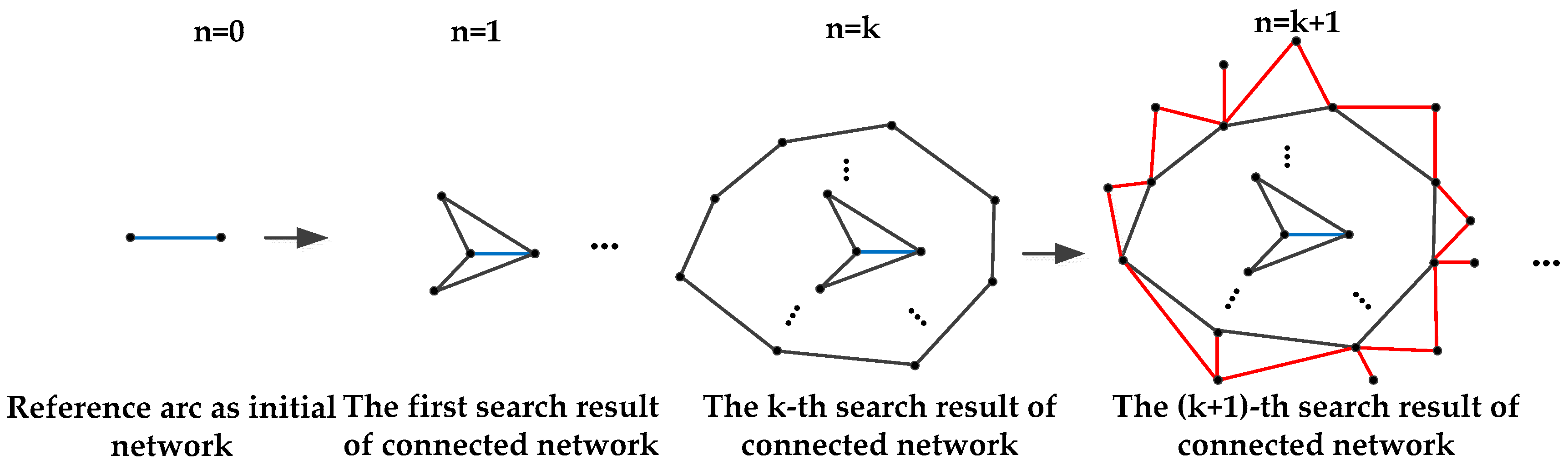
The identification of the largest connected network is an iteration process. We start with one reference arc in the largest connected network as the initial network. The iteration involves the step of enlarging the network by adding SPS arcs directly connected with the current network. The iteration ends until no directly connected SPS arcs can be found. The searching process is demonstrated in Figure 3.
Assuming that the largest connected network is searched out after iterations and there are arcs and SPSs in the searching result of connected network, then the largest connected network contains SPS arcs and SPSs. The integration of the searched connected network can be modeled as follows:
where is the relative elevation of SPS arcs of the searched connected network; is the transformation matrix from SPS arcs to SPS points consisting of 0, −1, 1; and is the absolute elevation of SPS points in the searched connected network:
where is singular because the rank is always . Assuming that is chosen as reference, the corresponding column in is removed, and then becomes a full-rank matrix.
The WLS estimator is typically used to integrate the absolute elevation from the largest connected network in the first-tier network, as shown in [29]. However, it inevitably brings about huge computation burden caused by the time-consuming inversion of high dimension matrix , especially for large network inversion. To solve this problem, we propose a network decomposition WLS (ND-WLS) estimator to accelerate the integration. The largest connected network can be decomposed into levels of connected networks by searching iterations, as shown in Figure 3. The integration of the searched connected network can be sped up based on the integration result of the searched connected network. The detailed implementation of the ND-WLS estimator is demonstrated below.
The searched connected network with arcs and SPSs can be modeled as follows:
where and . The front rows and columns of is the same as . Then, can be decomposed as follows:
where is a matrix with values from line to line and the front columns of . is a matrix with values from line to line and column to column of .
Correspondingly, Equation (12) can be transformed into the following model:
If we define and , then Equation (14) can be rewritten as follows:
Combing with the employment of WLS estimator, the solution of Equation (15) can be given by the following:
where represents the weight matrix; and is the weight coefficient of the SPS arc of , with being the RSR value of the SPS arc of .
Lastly, the integration result of the searched connected network can be given as follows:
The integration of the network integration is based on the integration of the connected network. Therefore, the robustness of the initial integration is ensured. In this case, we start from the searched connected network with not too few reliable arcs, typically one-half of the total reliable arcs in the largest connected network, which is initially integrated by the WLS estimator. The flow of ND-WLS is outlined below.
| ND-WLS estimator: Initialize : we start from the searched connected network with SPS arcs and SPSs. We apply WLS estimator to retrieve . 1. Let , the searched connected network with SPS arcs and SPSs can be retrieved: . Stop when (no new directly connected arcs found). |
2.2.3. Second-Tier Network Construction and Detection of the Remaining PSs
The second-tier network is constructed to detect DPSs and the remaining SPSs. Amplitude dispersion cannot be employed to select DPSs because DPS pixels do not have the characteristic of temporal amplitude stability. Moreover, SPSs are not always temporally stable in amplitude. Instead, amplitude threshold is employed to select PS candidates (PSCs) because both SPSs and DPSs show the property of high reflectivity. We remove the reliable SPSs detected in the first-tier network to select the remaining PSCs (RPSCs). Then, we construct arcs by connecting the RPSCs with the nearest reliable SPSs of the expanded largest connected network in the first-tier network, thereby forming the second-tier network. The construction of the second-tier network is based on the reliable SPSs of the largest connected network in the first-tier network. The SPS-DPS arc might be formed by connecting the SPS in the first-tier network and the DPS in the second-tier network. Similarly, the APS calibration in the second-tier network is performed by removing the phase of the reliable SPSs of the largest connected network in the first-tier network. When the APS is effectively calibrated to a small scale, the SPS-DPS arc can be focused like a DPS.
After the APS is calibrated, we employ the BF-based SGLRTC to detect all the DPSs and the remaining SPSs. If the relative tomographic signal of an arc in the second-tier network is detected as a SPS, we consider the RPSC at the arc as a true SPS. If the relative tomographic signal of an arc in the second-tier network is detected as a DPS, we consider the RPSC as a true DPS. The relative elevation estimation in the second-tier network can also be acquired. The estimates are relative to the reference SPSs in the first-tier network, so we can directly add the elevation of the reference SPSs that have been obtained in the first-tier network to retrieve the absolute elevation of SPSs and DPSs detected in the second-tier network. In addition, the RSR are computed to evaluate the goodness of the estimation for all arcs in the second-tier network. RSR thresholding is used to reject SPSs and DPSs with low-quality estimation. As the largest connected network is expanded with more manual structure information subtracted in the first-tier network, more reliable SPS and DPSs can be robustly detected by the novel two-tier network.
3. Results
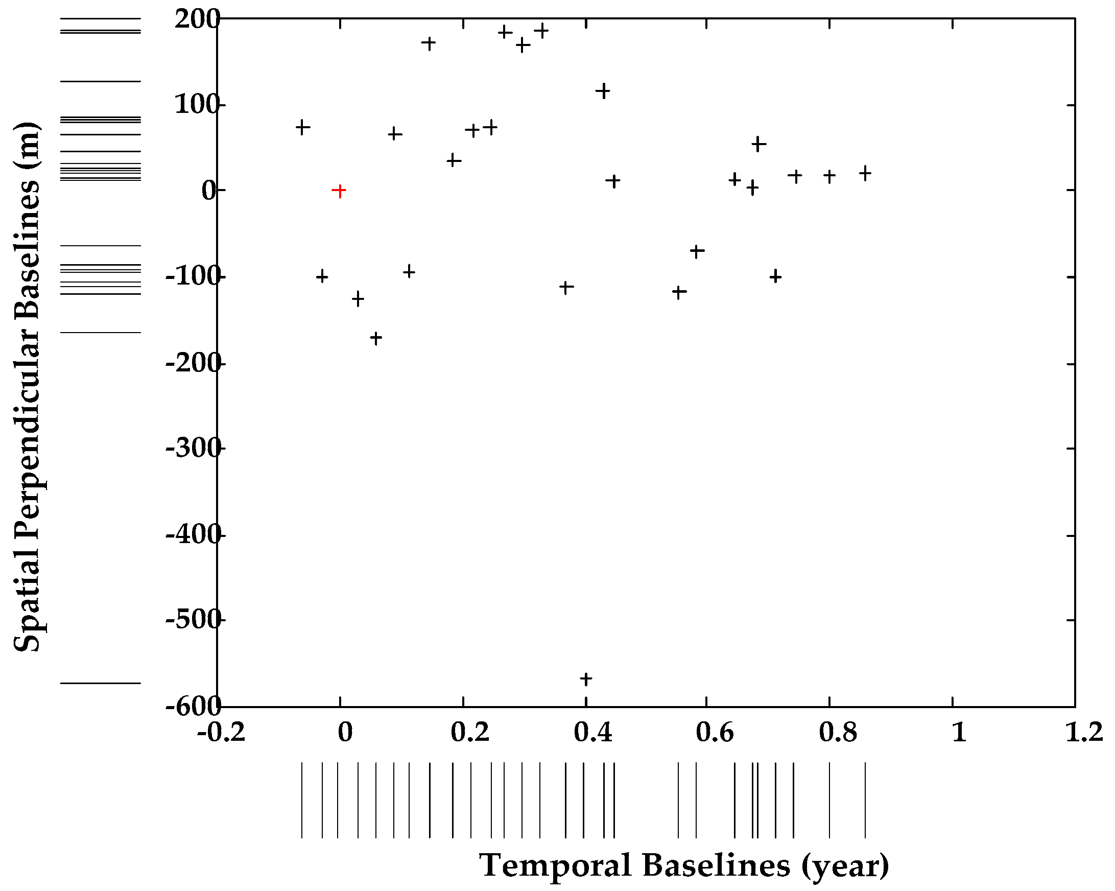
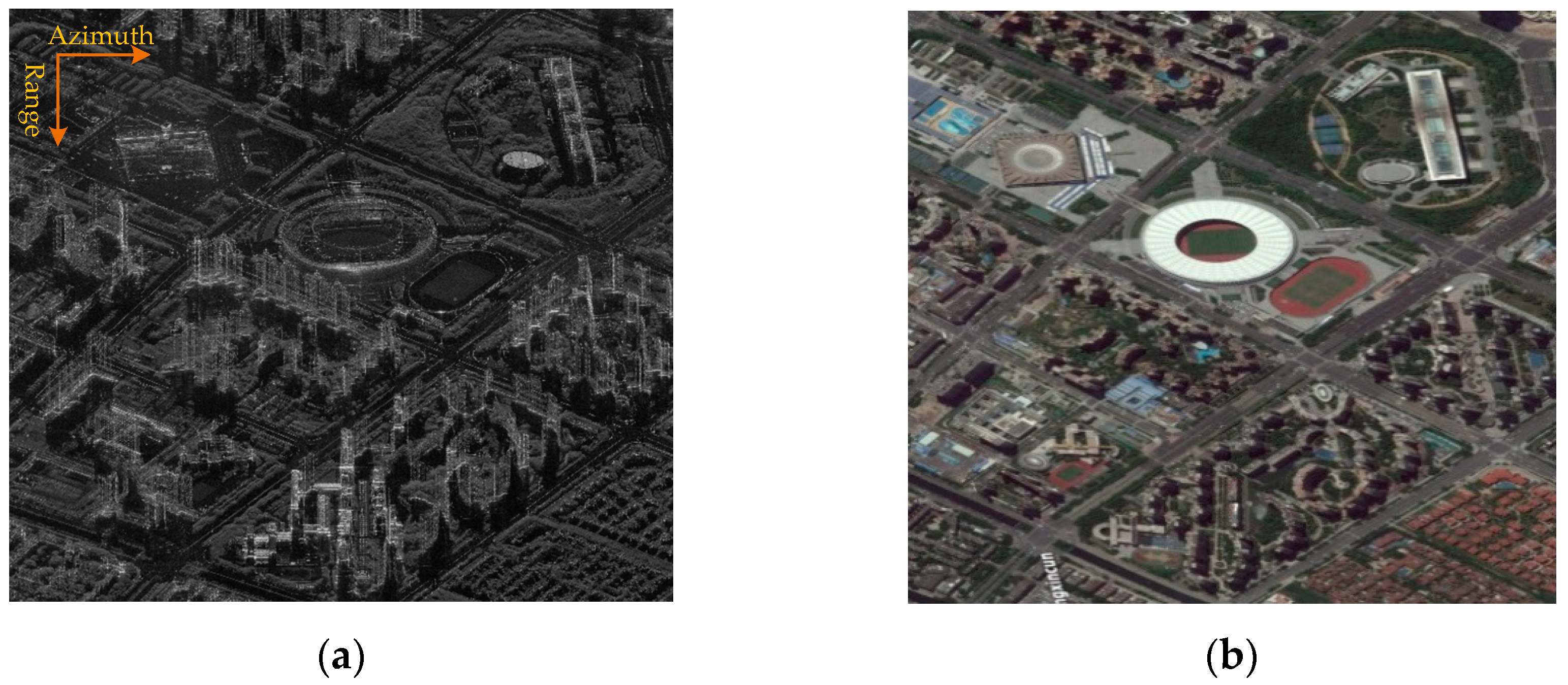
We conducted the proposed new approaches on a stack of 27 spotlight mode TerraSAR-X images acquired by repeat-pass mode from January 5, 2016 to November 30, 2016. The acquisition repeat cycle for TerraSAR-X was 11 days. The parameters of the acquired SAR data are shown in Table 1. The span of spatial perpendicular baselines for all acquisitions was about 752.8 m. As shown in Figure 4, the distribution of the temporal and spatial perpendicular baselines relative to the master acquisition was nonuniform (the master acquisition is marked with the red plus sign). The test site was an urban area, approximately 1 km × 1 km, of the Baoan district in Shenzhen, China. The mean calibrated intensity image and the corresponding Google image of the test site is shown in Figure 5.
If the spatial perpendicular baselines are uniformly distributed, the Rayleigh resolution in elevation would be as follows:
where = 3.1 cm is the wavelength, = 645.6 km is the center slant range, and = 752.8 m is the span of the spatial perpendicular baselines. The corresponding Rayleigh resolution in height would be about 7.5 m at an incidence angle = 39.48°.
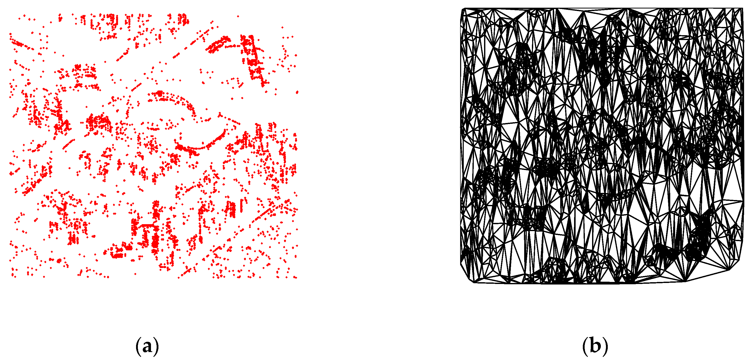
We used an amplitude dispersion of 0.12, and 12,975 pixels were then selected as SPSCs, as shown in Figure 6a. The selected SPSCs were distributed in the whole scene. As sketched in Figure 6b, Delaunay triangulation was used to construct the first-tier network and to calibrate the APS of selected SPSCs. There were in total 38,900 arcs in the first-tier network.
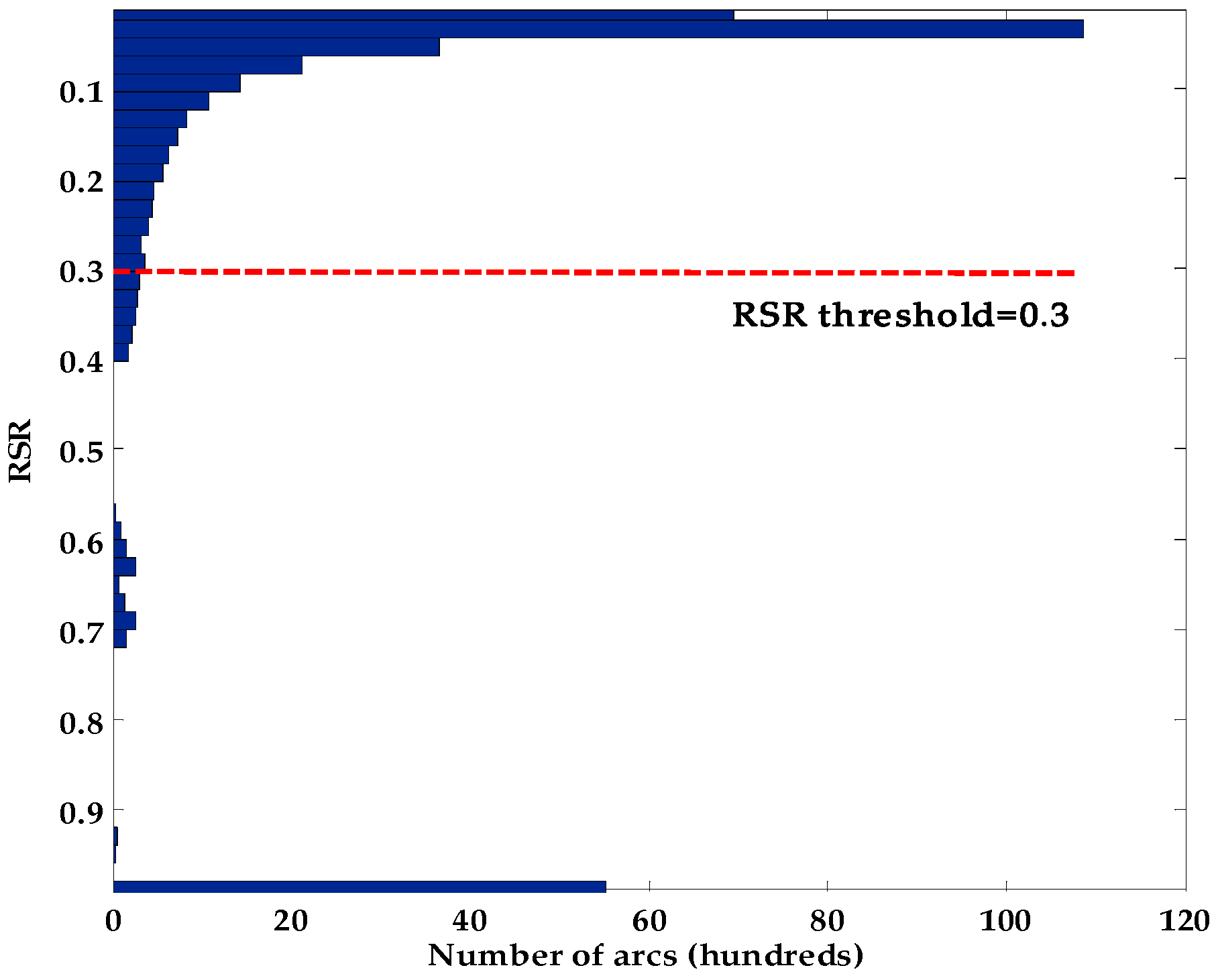
Thereafter, a distance threshold of 300 m was used, and arcs longer than 300 m were then discarded. Next, we applied the BF-based SGLRTC to select SPS arcs and acquire the relative height information. When applying the BF-based SGLRTC method for detecting SPSs or DPSs, the estimated normalized energy for the first scatterer was 0.6, and the normalized energy for the second scatterer (after the cancelation of the first scatterer) was 0.4. The RSR values for all arcs in the first-tier network were computed, as shown in Figure 7. We found that 84.5% of the RSR values were smaller than 0.4, indicating that the APS of most of the arcs in the first-tier network had been effectively calibrated. In order to preserve the SPS arcs that had their APS effectively calibrated and subtract SPSs with accurate relative estimation, an RSR threshold of 0.3 was used for network adjustment, and, reliable SPS arcs with RSR values smaller than 0.3 were preserved. As a result, 29,922 SPS arcs (10,076 SPSs) were preserved, accounting for approximately 77% of the entire first-tier network.
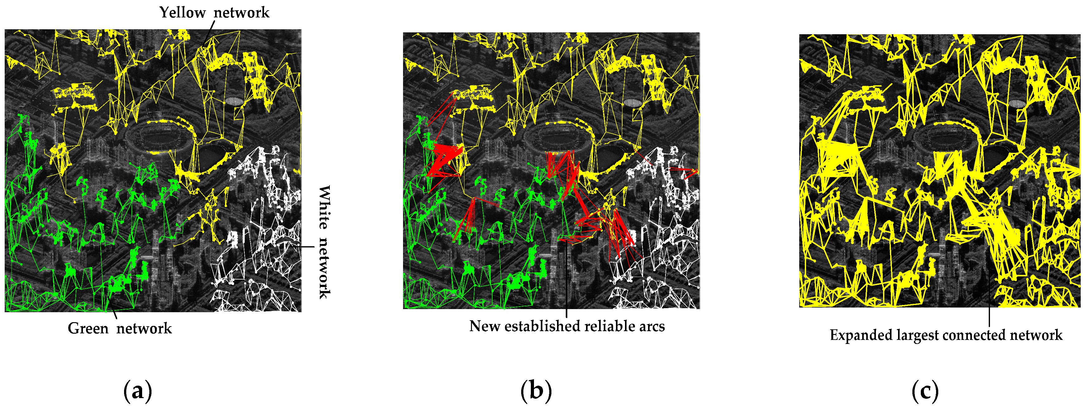
There were three main isolated networks after network adjustment of the first-tier network, as shown in Figure 8a. Tiny networks with very few SPSs (typically 500) were omitted. If smaller distance threshold and smaller RSR threshold are taken, reliable SPS arcs with higher quality estimation will be selected. Otherwise, the consistency of the first-tier network will be destroyed more seriously, yielding more isolated networks. Therefore, the distance threshold and RSR threshold should be appropriate to balance the estimation quality and the condition of network consistency. The yellow connected network, which was the largest network, contained 10,662 SPS arcs and 4392 SPSs. The green network and the white network contained 10,478 SPS arcs and 4416 SPSs in total. The yellow largest network contained much useful information of manual structures, but the green and white networks also contained useful structure information of the test site. If only the yellow network were to be utilized, the height information of the area covered by the green network and the white network would have been absent. Therefore, to subtract more useful structure information in the first-tier network, we attempted to establish reliable SPS arcs among the three main isolated networks. As shown in Figure 8b, 2111 reliable SPS arcs (red) were established to connect these three main networks. Through the establishment of reliable arcs, the three main isolated networks were connected together. The expanded largest connected network was the combination of these three main networks and newly established reliable arcs, as shown in Figure 8c. There were in total 23,251 arcs and 8808 SPSs in the expanded largest connected network. The SPSs in the expanded largest connected network was uniformly distributed in the whole test site.
The utilization rate of true SPSs for the original largest connected network and the expanded largest connected network are shown in Table 2. The number of true SPSs utilized in the expanded largest network was nearly twice the number of SPSs utilized in the original largest network. Compared with the original largest connected network, the utilization rate of true SPSs for the expanded largest network improved about 43.77%.
In addition, in order to intuitively show the effectiveness of APS calibration in the first-tier network, we randomly chose two reliable SPS arcs in the largest connected network as an example. We could judge whether the APS was effectively calibrated by the focusing condition of the reconstructed reflectivity profile. Figure 9a manifests the reflectivity profile of ideal measurements with the same baseline distribution shown in Figure 4 and without error interference for an SPS point with . The high sidelobes were caused by the nonuniform distribution of spatial perpendicular baselines. Figure 9b,c show the reflectivity profiles of the two reliable SPS arcs, including SPS pairs. P1 and P2 show that the measurements of the two connected SPSs of arc 1 or arc 2 could not be focused because the measurements were severely influenced by large-scale APS. In contrast, P3 shows that the relative measurements of arc 1 or arc 2 with APS calibrated could be focused, which had approximately identical level of highest sidelobe as that in Figure 8a. This indicated that the APS was effectively calibrated to a small scale in the first-tier network.
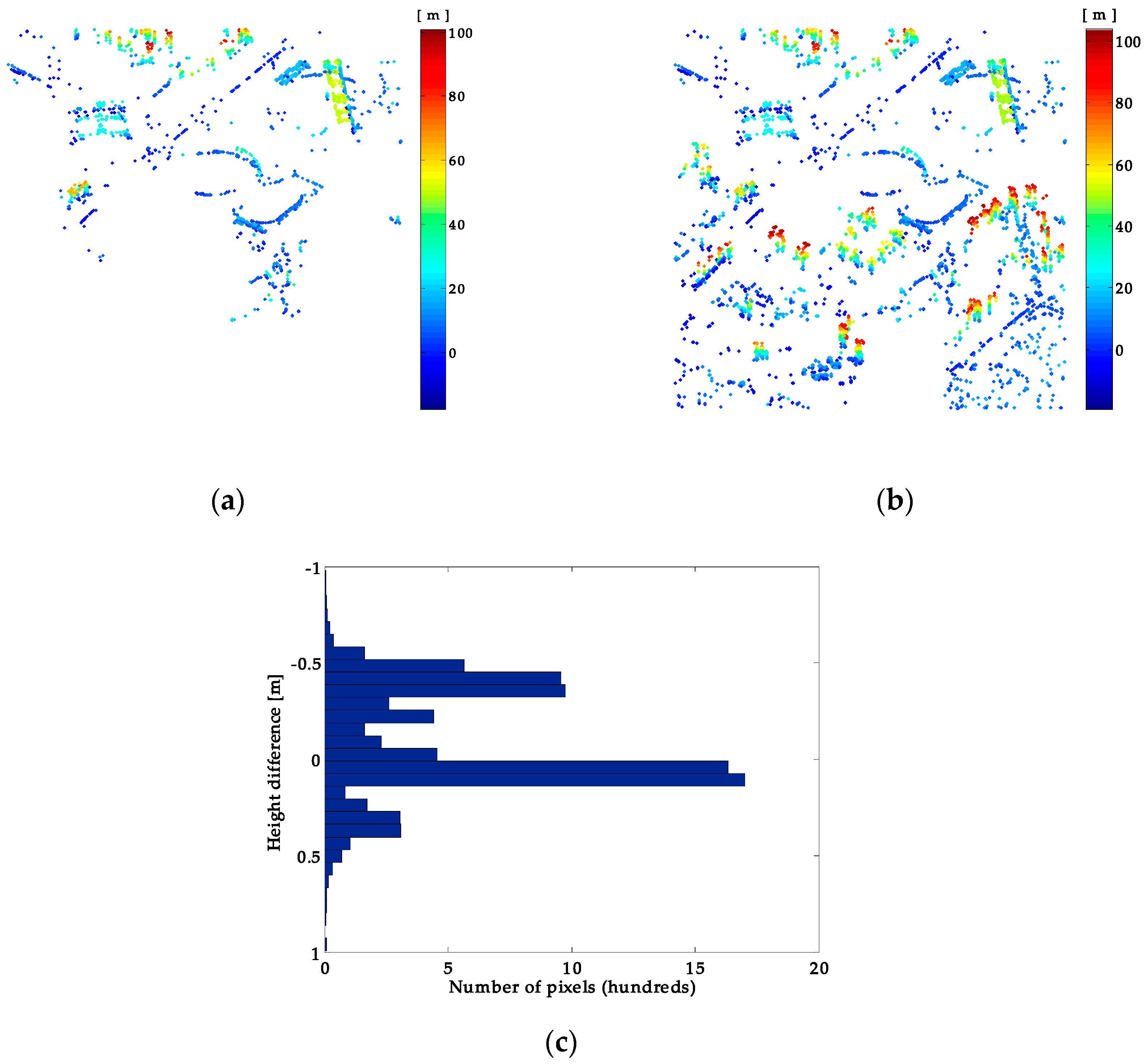
After acquiring the relative elevation of all reliable SPS arcs, we integrated them to retrieve the absolute height over one reference point. The ND-WLS estimator was used to integrate the relative height of reliable SPSs from the connected network. The estimated height of SPSs in the original largest connected network and in the expanded largest connected network is presented in Figure 10a,b, respectively. It is clear that the height information of the area covered by the green and white networks shown in Figure 8a was absent when the original largest connected network was utilized. In contrast, height information of nearly the whole test site could be acquired by utilizing the expanded largest connected network. Furthermore, in order to reflect the accuracy of ND-WLS estimator, the histogram of the height difference between the height retrieved by the ND-WLS estimator and the WLS estimator from the expanded largest connected network is shown in Figure 10c. As can be seen, the height difference was far smaller than the Rayleigh resolution in height, indicating that the ND-WLS estimator had the same high precision as the WLS estimator. In addition, Table 3 shows the computation time of retrieving absolute height from the expanded largest connected network by the WLS estimator and the ND-WLS estimator. Under the same computation condition, the ND-WLS estimator was much faster than the WLS estimator. Overall, the integration process could be accelerated with precision maintenance by employing the ND-WLS estimator, which proved to be quite useful for large network inversion.
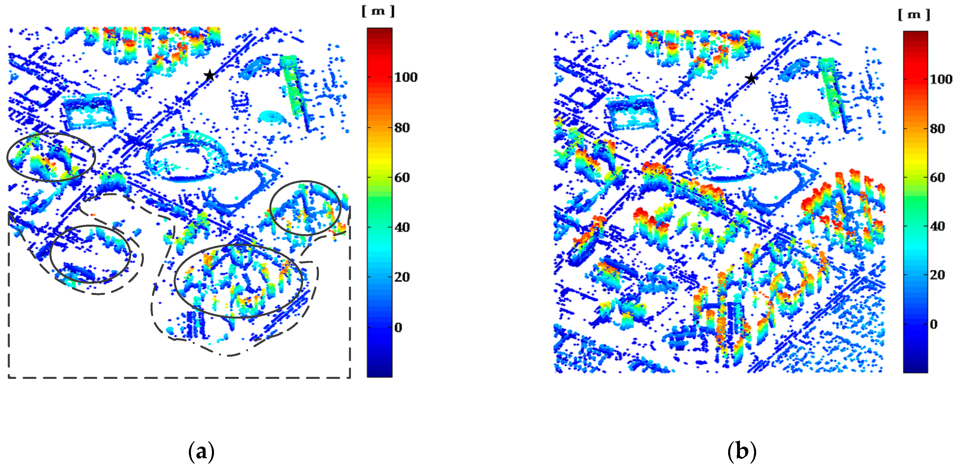
The second-tier network was constructed on the basis of the largest connected network utilized in the first-tier network. When the original largest connected network was utilized, 100,335 SPSs and 201 DPSs could be detected in the second-tier network. When the expanded largest connected network was utilized, 183,815 SPSs and 386 DPSs could be detected in the second-tier network. Compared with the traditional two-tier network, the number of SPSs and DPSs detected by the novel two-tier network was more than 80%. The number of detected DPSs in this area was few, mainly from roof and facade of tall buildings, so we have not shown them separately in this paper. We merged the SPSs with the dominant PSs of DPSs and chose one SPS, marked as black star on the road, as the reference point. The estimated height of the merged PSs by traditional two-tier network is shown in Figure 11a. The height information of the area covered by the black dotted box was absent, and information about the height of many buildings in the ellipse was not fully acquired due to the absence of sufficient reference SPSs in these areas. The estimated height of merged PSs by the novel two-tier network is shown in Figure 11b. It is obvious that the height information of all the buildings in the test site could be acquired by the novel two-tier network.
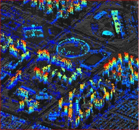
In Figure 12, we display 25% of the total PSs detected in the novel two-tier network and visualize them in the mean calibrated SAR intensity image. The 3D distribution of the urban area, including the gymnasium, district government, and residential buildings, can be clearly seen. Such dense TomoSAR point clouds can be further utilized for reconstructing dynamic city models. Overall, the effectiveness of the new approaches for robust and efficient detection of PSs in SAR tomography was verified by this experiment.
4. Conclusions
In this paper, we propose new approaches based on a novel two-tier network for robust and efficient detection of PSs. In the first-tier network, a Delaunay triangulation network is constructed, and the APS is calibrated. After APS calibration, the BF-based SGLRTC is employed for the detection of PSs. The RSR estimator is proposed to evaluate the effectiveness of APS calibration and to select reliable PSs with accurate estimation. In addition, we propose to establish reliable arcs among the main isolated networks to subtract more useful structure information in the first-tier network. In this way, more SPSs and DPSs can be detected by the novel two-tier network. Moreover, rather than the WLS estimator, the ND-WLS estimator is proposed to accelerate the retrieval of absolute estimation with precision maintenance, which is quite useful for large network inversion.
The temporally uncorrelated APS has a big impact on all repeat-pass SAR systems working with different frequencies other than the X-band in SAR tomography. More testing is required to show the significance of APS calibration and the effectiveness of the proposed new approaches.
Author Contributions
Conceptualization, X.Z. and A.Y.; formal analysis, X.Z.; funding acquisition, Z.D. and M.W.; investigation, X.Z. and D.L.; methodology, X.Z. and A.Y.; resources, A.Y. and Z.D.; supervision, Y.Z., Z.D., and M.W.; validation, X.Z.; writing—review and editing, X.Z. and A.Y.
Funding
This work was supported by the National Natural Science Foundation of China under grant number 61771478.
Acknowledgments
We will particularly like to acknowledge the support of the German Aerospace Center (DLR) for providing high-resolution TerraSAR-X data.
Conflicts of Interest
The authors declare no conflict of interest.
References
- Cigna, F.; Lasaponara, R.; Masini, N.; Milillo, P.; Tapete, D. Persistent Scatterer Interferometry Processing of COSMO-SkyMed Stripmap HIMAGE Time Series to Depict Deformation of the Historic Centre of Rome, Italy. Remote Sens. 2014, 6, 12593–12618. [Google Scholar] [CrossRef]
- Perissin, D.; Prati, C.; Rocca, F.; Teng, W. PSInSAR Analysis over the Three Gorges Dam and Urban areas in China. In Proceedings of the Urban Remote Sensing Event, Shanghai, China, 20–22 May 2009; pp. 1–5. [Google Scholar]
- Perissin, D.; Prati, C.; Rocca, F. ASAR parallel-track PS analysis in urban sites. In Proceedings of the IEEE International Geoscience and Remote Sensing Symposium (IGARSS), Barcelona, Spain, 23–28 July 2007; pp. 1167–1170. [Google Scholar]
- Milillo, P.; Roland, B.; Lundgren, P.; Salzer, J.; Milillo, G. Space geodetic monitoring of engineered structures: The ongoing destabilization of mosul dam, Iraq. Sci. Rep. 2016, 6, 37408. [Google Scholar] [CrossRef] [PubMed]
- Milillo, P.; Perissin, D.; Salzer, J.T.; Lundgren, P.; Lacava, G.; Milillo, G. Monitoring dam structural health from space: Insights from novel insar techniques and multi-parametric modeling applied to the pertusillo dam basilicata, Italy. Int. J. Appl. Earth Obs. Geoinf. 2016, 52, 221–229. [Google Scholar] [CrossRef]
- Lombardini, F.; Pardini, M. 3-D SAR Tomography: The Multibaseline Sector Interpolation Approach. IEEE Geosci. Remote Sens. Lett. 2008, 5, 630–634. [Google Scholar] [CrossRef]
- Zhu, X.X.; Bamler, R. Very High Resolution Spaceborne SAR Tomography in Urban Environment. IEEE Trans. Geosci. Remote Sens. 2010, 48, 4296–4308. [Google Scholar] [CrossRef] [Green Version]
- Zhu, X.X.; Yuanyuan, W.; Sina, M.; Nan, G. A Review of Ten-Year Advances of Multi-Baseline SAR Interferometry Using TerraSAR-X Data. Remote Sens. 2018, 10, 1374. [Google Scholar] [CrossRef]
- Reigber, A.; Moreira, A. First demonstration of airborne SAR tomography using multibaseline L-band data. IEEE Trans. Geosci. Remote Sens. 2000, 38, 2142–2152. [Google Scholar] [CrossRef]
- Fornaro, G.; Serafino, F. Imaging of Single and Double Scatterers in Urban Areas via SAR Tomography. IEEE Trans. Geosci. Remote Sens. 2006, 44, 3497–3505. [Google Scholar] [CrossRef]
- Werninghaus, R.; Buckreuss, S. The TerraSAR-X Mission and System Design. IEEE Trans. Geosci. Remote Sens. 2010, 48, 606–614. [Google Scholar] [CrossRef] [Green Version]
- Covello, F.; Battazza, F.; Coletta, A.; Lopinto, E.; Fiorentino, C.; Pietranera, L. COSMO-SkyMed an existing opportunity for observing the Earth. J. Geodyn. 2010, 49, 171–180. [Google Scholar] [CrossRef] [Green Version]
- Tebaldini, S. Single and Multipolarimetric SAR Tomography of Forested Areas: A Parametric Approach. IEEE Trans. Geosci. Remote Sens. 2010, 48, 2375–2387. [Google Scholar] [CrossRef]
- Tebaldini, S.; Rocca, F.; Guarnieri, A.M. Model Based SAR Tomography of Forested Areas. In Proceedings of the IEEE International Geoscience and Remote Sensing Symposium (IGARSS), Boston, MA, USA, 7–11 July 2008; pp. 593–596. [Google Scholar]
- Ferro-Famil, L.; Tebaldini, S.; Davy, M. Very high-resolution three-dimensional imaging of natural environments using a tomographic ground-based SAR system. In Proceedings of the European Conference on Antennas and Propagation (EuCAP), The Hague, The Netherlands, 6–11 April 2014; pp. 3221–3224. [Google Scholar]
- Ferro-Famil, L.; Leconte, C.; Boutet, F.; Phan, X.V.; Gay, M.; Durand, Y. PoSAR: A VHR tomographic GB-SAR system application to snow cover 3-D imaging at X and Ku bands. In Proceedings of the Radar Conference, Amsterdam, The Netherlands, 31 October–2 November 2012; pp. 130–133. [Google Scholar]
- Colesanti, C.; Ferretti, A.; Novali, F.; Prati, C.; Rocca, F. SAR monitoring of progressive and seasonal ground deformation using the permanent scatterers technique. IEEE Trans. Geosci. Remote Sens. 2003, 41, 1685–1701. [Google Scholar] [CrossRef]
- Ferretti, A.; Bianchi, M.; Prati, C.; Rocca, F. Higher-Order Permanent Scatterers Analysis. EURASIP J. Appl. Signal Process. 2005, 2005, 3231–3242. [Google Scholar] [CrossRef] [Green Version]
- De Maio, A.; Fornaro, G.; Pauciullo, A. Detection of Single Scatterers in Multidimensional SAR Imaging. IEEE Trans. Geosci. Remote Sens. 2009, 47, 2284–2297. [Google Scholar] [CrossRef]
- Pauciullo, A.; Reale, D.; De Maio, A.; Fornaro, G. Detection of Double Scatterers in SAR Tomography. IEEE Trans. Geosci. Remote Sens. 2012, 50, 3567–3586. [Google Scholar] [CrossRef]
- Kumar, S. Atmosphere Effects Correction. Estimation and Correction of Tropospheric and Ionospheric Effects on Differential SAR Interferograms. Master’s Thesis, University of Twente, Enschede, The Netherlands, 2011. [Google Scholar]
- Dwyer, M.J.; Schmidt, G. The MODIS Reprojection Tool; Earth Science Satellite Remote Sensing; Springer: Berlin/Heidelberg, Germany, 2006; pp. 162–177. [Google Scholar]
- Lee, H.B.; Kim, Y. Assessment of GPS global ionosphere maps (GIM) by comparison between CODE GIM and TOPEX/Jason TEC data: Ionospheric perspective. J. Geophys. Res. Space Phys. 2010, 115. [Google Scholar] [CrossRef] [Green Version]
- Global Ionosphere Maps Produced by CODE. Available online: http://www.aiub.unibe.ch/content/research/gnss/code_research/igs/global_ionosphere_maps_produced_by_code/index_eng.html (accessed on 28 December 2018).
- Ferretti, A.; Prati, C.; Rocca, F. Permanent scatterers in SAR interferometry. IEEE Trans. Geosci. Remote Sens. 2001, 39, 8–20. [Google Scholar] [CrossRef] [Green Version]
- Siddique, M.A.; Wegmüller, U.; Hajnsek, I.; Frey, O. Single-Look SAR Tomography as an Add-On to PSI for Improved Deformation Analysis in Urban Areas. IEEE Trans. Geosci. Remote Sens. 2016, 54, 6119–6137. [Google Scholar] [CrossRef]
- Moreira, A.; Prats-Iraola, P.; Younis, M.; Krieger, G.; Hajnsek, I.; Papathanassiou, K.P. A tutorial on synthetic aperture radar. IEEE Geosci. Remote Sens. Mag. 2013, 1, 6–43. [Google Scholar] [CrossRef] [Green Version]
- Crosetto, M.; Monserrat, O. Persistent Scatterer Interferometry: A review. ISPRS J. Photogramm. Remote Sens. 2016, 115, 78–89. [Google Scholar] [CrossRef] [Green Version]
- Ma, P.; Hui, L. Robust Detection of Single and Double Persistent Scatterers in Urban Built Environments. IEEE Trans. Geosci. Remote Sens. 2016, 54, 2124–2139. [Google Scholar] [CrossRef]
- Jenq, Y.C. High-precision sinusoidal frequency estimator based on weighted least square method. IEEE Trans. Instrum. Meas. 1987, 36, 124–127. [Google Scholar] [CrossRef]
- Van Trees, H.L. Detection, Estimation, and Modulation Theory: Pt. 1.: Detection, Estimation, and Linear Modulation; John Wiley & Sons: Hoboken, NJ, USA, 2004. [Google Scholar]
- Fornaro, G.; Serafino, F.; Soldovieri, F. Three-dimensional focusing with multipass SAR data. IEEE Trans. Geosci. Remote Sens. 2003, 41, 507–517. [Google Scholar] [CrossRef]
- Lombardini, F.; Montanari, M.; Gini, F. Reflectivity estimation for multibaseline interferometric radar imaging of layover extended sources. IEEE Trans. Signal Process. 2003, 51, 1508–1519. [Google Scholar] [CrossRef]
- Olivier, D.H.; Ronny, H.; Nicolas, W.; Olaf, H. Exploiting SAR Tomography for Supervised Land-Cover Classification. Remote Sens. 2018, 10, 1742. [Google Scholar]
- Noferini, L.; Pieraccini, M.; Mecatti, D.; Luzi, G.; Atzeni, C.; Tamburini, A. Permanent scatterers analysis for atmospheric correction in ground-based SAR interferometry. IEEE Trans. Geosci. Remote Sens. 2005, 43, 1459–1471. [Google Scholar] [CrossRef]
- Frey, O.; Hajnsek, I.; Wegmuller, U. Spaceborne SAR Tomography in Urban Areas. In Proceedings of the 2013 IEEE International Geoscience and Remote Sensing Symposium, Melbourne, Australia, 21–26 July 2013; pp. 69–72. [Google Scholar]
- Fornaro, G.; Lombardini, F.; Serafino, F. Three-dimensional multipass SAR focusing: Experiments with long-term spaceborne data. IEEE Trans. Geosci. Remote Sens. 2005, 43, 702–714. [Google Scholar] [CrossRef]
- Zhu, X.X.; Bamler, R. Tomographic SAR Inversion by L1-norm Regularization—The Compressive Sensing Approach. IEEE Trans. Geosci. Remote Sens. 2010, 48, 3839–3846. [Google Scholar] [CrossRef]
- Fornaro, G.; Lombardini, F.; Pauciullo, A.; Reale, D.; Viviani, F. Tomographic Processing of Interferometric SAR Data: Developments, applications, and future research perspectives. IEEE Signal Process. Mag. 2014, 31, 41–50. [Google Scholar] [CrossRef]
- Zhu, X.X.; Bamler, R. Super-Resolution Power and Robustness of Compressive Sensing for Spectral Estimation with Application to Spaceborne Tomographic SAR. IEEE Trans. Geosci. Remote Sens. 2012, 50, 247–258. [Google Scholar] [CrossRef]
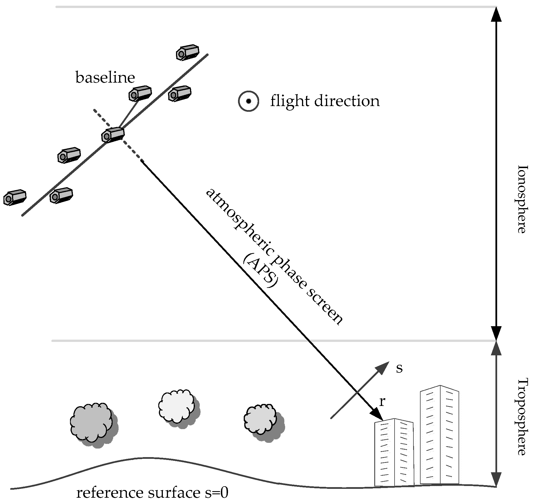
Figure 1.
Multipass synthetic aperture radar (SAR) geometry in the range–elevation plane. The coordinate is referred to as elevation. The satellite flies into the plane and looks to its right.
Figure 1.
Multipass synthetic aperture radar (SAR) geometry in the range–elevation plane. The coordinate is referred to as elevation. The satellite flies into the plane and looks to its right.

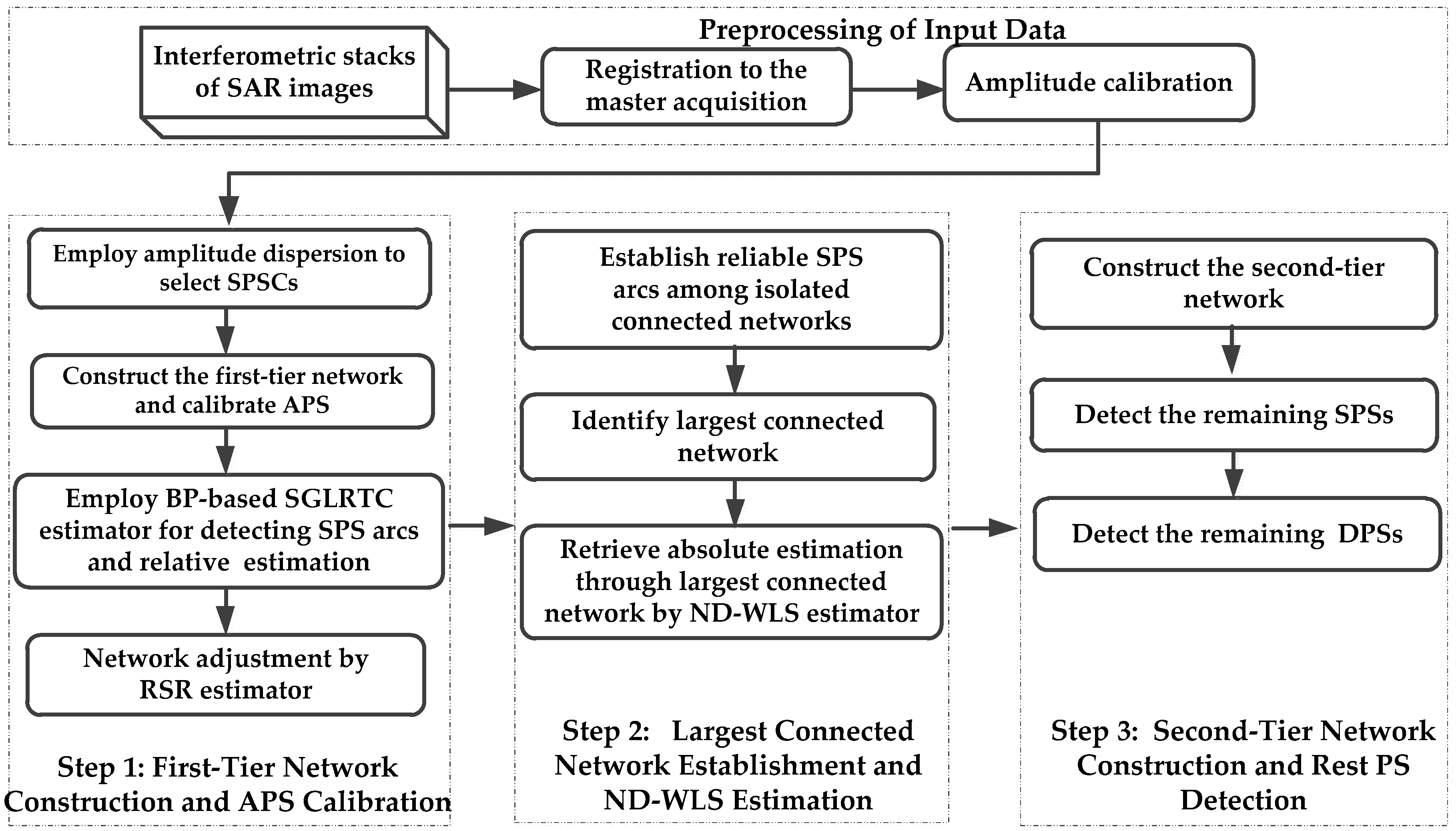
Figure 2.
Flowchart of the new approaches for robust and efficient detection of persistent scatterers (PSs). Abbreviations: SPS, single persistent scatterer; DPS, double persistent scatterer; SPSC, SPS candidate; APS, atmospheric phase screen; BP, Beam-Forming; SGLRTC, sequential generalized likelihood ratio test with cancellation; RSR: residue-to-signal ratio; ND-WLS, network decomposition weighted least square.

Figure 3.
The searching process of the largest connected network.

Figure 4.
Distribution of the temporal baselines and spatial perpendicular baselines.

Figure 5.
(a) The mean calibrated intensity image of the test site; (b) the Google Earth snapshot of the same area.
Figure 5.
(a) The mean calibrated intensity image of the test site; (b) the Google Earth snapshot of the same area.

Figure 6.
SPSCs and the first-tier network (a) SPSCs marked with red solid points; (b) first-tier network constructed by Delaunay triangulation.
Figure 6.
SPSCs and the first-tier network (a) SPSCs marked with red solid points; (b) first-tier network constructed by Delaunay triangulation.

Figure 7.
RSR values for all arcs in the first-tier network.

Figure 8.
The process of establishing the largest connected network. (a) The main isolated networks after network adjustment; (b) establishing reliable arcs among the main isolated networks; (c) the expanded largest connected network.
Figure 8.
The process of establishing the largest connected network. (a) The main isolated networks after network adjustment; (b) establishing reliable arcs among the main isolated networks; (c) the expanded largest connected network.

Figure 9.
Reconstructed reflectivity profiles. (a) The ideal reflectivity profile with no phase error; (b) the reconstructed reflectivity of arc 1; (c) the reconstructed reflectivity of arc 2. P1: the reconstructed reflectivity profile of the first SPS point of one SPS arc without APS calibration. P2: the reconstructed reflectivity profile of the second SPS point of one SPS arc without APS calibration. P3: the reconstructed reflectivity profile of the relative measurements of an SPS arc after APS calibration.

Figure 10.
Estimated height of reliable SPSs and height difference histogram. (a) Estimated height of SPSs in the original largest connected network by ND-WLS estimator; (b) estimated height of SPSs in the expanded largest connected network by ND-WLS estimator; (c) the histogram of height difference between the height retrieved by ND-WLS estimator and WLS estimator.

Figure 11.
Estimated height of merged PSs. (a) Estimated height of merged PSs by traditional two-tier network; (b) estimated height of merged PSs by novel two-tier network.
Figure 11.
Estimated height of merged PSs. (a) Estimated height of merged PSs by traditional two-tier network; (b) estimated height of merged PSs by novel two-tier network.

Figure 12.
Estimated height visualized in mean calibrated SAR intensity image. The color bar is the same as that in Figure 11b.
Figure 12.
Estimated height visualized in mean calibrated SAR intensity image. The color bar is the same as that in Figure 11b.


Table 1.
Parameters of the TerraSAR-X acquisitions in spotlight mode.
| System Parameters | Value |
|---|---|
| Center slant range | 645.6 km |
| Orbit direction | Descending |
| Incidence angle | 39.48° |
| Carrier frequency | 9.65 GHz |
| Wavelength | 0.03 cm |
| Chirp bandwidth | 300 MHz |
| Azimuth resolution | 0.167 m |
| Range resolution | 0.454 m |
| Span of spatial Perpendicular baseline | 752.8 m |
Table 2.
Utilization rate of true SPSs between original and expanded largest networks.
| Largest Connected Network | Original | Expanded | Gain |
|---|---|---|---|
| Number of true SPSs | 4392 | 8808 | 4410 |
| Utilization rate | 43.59% | 87.36% | 43.77% |
Table 3.
Computation time by WLS and ND-WLS.
| Estimator | WLS | ND-WLS |
|---|---|---|
| Computation time/s | 208.93 | 45.74 |
© 2019 by the authors. Licensee MDPI, Basel, Switzerland. This article is an open access article distributed under the terms and conditions of the Creative Commons Attribution (CC BY) license (http://creativecommons.org/licenses/by/4.0/).
Share and Cite
MDPI and ACS Style
Zhu, X.; Dong, Z.; Yu, A.; Wu, M.; Li, D.; Zhang, Y. New Approaches for Robust and Efficient Detection of Persistent Scatterers in SAR Tomography. Remote Sens. 2019, 11, 356. https://0-doi-org.brum.beds.ac.uk/10.3390/rs11030356
AMA Style
Zhu X, Dong Z, Yu A, Wu M, Li D, Zhang Y. New Approaches for Robust and Efficient Detection of Persistent Scatterers in SAR Tomography. Remote Sensing. 2019; 11(3):356. https://0-doi-org.brum.beds.ac.uk/10.3390/rs11030356
Chicago/Turabian StyleZhu, Xiaoxiang, Zhen Dong, Anxi Yu, Manqing Wu, Dexin Li, and Yongsheng Zhang. 2019. "New Approaches for Robust and Efficient Detection of Persistent Scatterers in SAR Tomography" Remote Sensing 11, no. 3: 356. https://0-doi-org.brum.beds.ac.uk/10.3390/rs11030356
Note that from the first issue of 2016, this journal uses article numbers instead of page numbers. See further details here.