Object-Based Change Detection Using Multiple Classifiers and Multi-Scale Uncertainty Analysis

Abstract

The drawback of pixel-based change detection is that it neglects the spatial correlation with neighboring pixels and has a high commission ratio. In contrast, object-based change detection (OBCD) depends on the accuracy of the segmentation scale, which is of great significance in image analysis. Accordingly, an object-based approach for automatic change detection using multiple classifiers and multi-scale uncertainty analysis (OB-MMUA) in high-resolution (HR) remote sensing images is proposed in this paper. In this algorithm, the gray-level co-occurrence matrix (GLCM), morphological, and Gabor filter texture features are extracted to construct the input data, along with the spectral features, to utilize the respective advantages of the features and to compensate for the insufficient spectral information. In addition, random forest is used to select the features and determine the optimal feature vectors for the change detection. Change vector analysis (CVA) based on uncertainty analysis is then implemented to select the initial training samples. According to the diversity, support vector machine (SVM), k-nearest neighbor (KNN), and extra-trees (ExT) classifiers are then chosen as the base classifiers for Dempster-Shafer (D-S) evidence theory fusion, and unlabeled samples are selected using an active learning method with spatial information. Finally, multi-scale object-based D-S evidence theory fusion and uncertainty analysis is used to classify the difference image. To validate the proposed approach, we conducted experiments using multispectral images collected by the ZY-3 and GF-2 satellites. The experimental results confirmed the effectiveness and superiority of the proposed approach, which integrates the respective advantages of the pixel-based and object-based methods.

1. Introduction

Surface ecosystems and human social activities are dynamic and evolving [1]. With the acceleration of the human transformation of nature, especially the rapid advancement of urban construction in recent years, the surface coverage of the human living environment is rapidly changing. [2] Accurate access to surface change information is thus of great significance for better protection of the ecological environment, improvement of urban land management, and rational handling of the relationship and interaction between human life and the natural environment [3]. In remote sensing, change detection generally focuses on extracting the change information by analyzing multi-temporal images of the same geographical area [4]. Remote sensing Earth observation technology has the capability of large-scale, long-term, and periodic observation [5]. Therefore, change detection based on multi-temporal remote sensing images has been widely used in various fields, such as urban development [6], environmental monitoring, vegetation coverage studies [7], and land-use monitoring [8,9].

Change detection can be divided into pixel-based and object-based change detection (OBCD). Many scholars have proposed a variety of pixel-based change detection methods, including change vector analysis (CVA) [10,11], Markov random field (MRF)-based change detection [12], etc. With the development of machine learning, methods such as the extreme learning machine (ELM) algorithm [13], support vector machine (SVM) [14], random forest (RF) [15], k-nearest neighbor (KNN) [16], the multi-layer perceptron neural network (MLPNN) [17], and convolutional neural network (CNN) [18,19] have improved the accuracy of classification and change detection. However, a single classifier cannot detect all the change information in an image effectively. To address this issue, ensemble learning has been applied to the research and application of change detection and classification [20,21,22]. Du et al. (2012) [23] proposed an ensemble system based on multiple classifiers, and achieved good classification results. Zhang et al. (2017) [24] combined deep learning with feature change analysis for remote sensing image change detection, and the results confirmed that this new method is superior to the traditional methods. Despite the advantages of supervised classifiers in classification and change detection, they require training samples that are labeled beforehand. Manual selection of training samples can lead to incompleteness of the selected categories, and is also time-consuming. With the increase of the spatial resolution and the decrease of the spectral resolution in high spatial resolution images, the accuracy of change detection is degraded due to the same objects having different spectra [25]. Thus, the object-oriented technique has become one of the most popular methods for high spatial resolution images [26,27]. Wang et al. (2018) [28] proposed an OBCD method using multiple object features and multiple classifiers, which were integrated via weighted voting, achieving a superior performance. However, the accuracy of the change detection in object-based methods is directly influenced by the image segmentation.

Other scholars have studied the optimization of image segmentation. Tang et al. (2011) [29] proposed an OBCD algorithm based on the Kolmogorov-Smirnov (K-S) test, which uses the fractal network evolution algorithm (FNEA) for the image segmentation, and utilizes region merging to acquire the optimal segmentation scale. Peng et al. (2017) [30] proposed an OBCD method based on segmentation optimization and multi-feature fusion via the D-S evidence theory fusion. While a large number of scholars have proposed effective algorithms and theoretical models at both the pixel level and object level, there are still some limitations and difficulties. Pixel-based change detection algorithms can retain the boundary information of features, and object-based methods can reduce the noise in the image. A number of scholars have proved the effectiveness of combining pixel-based and object-based change detection methods [8]. Hao et al. (2016) [31] proposed an algorithm based on pixel-based classification and uncertainty analysis. Cao et al. (2014) [32] made an effective parallel integration of pixel-based and object-based methods, which improved the accuracy of change detection. Tan et al. (2018) [33] integrated heterogeneous segmentation and ensemble system pixel-based results to generate the final change map. However, these methods are all based on a single scale, or different scales that are treated independently. Accordingly, Zhang et al. (2017) [34] proposed an object-based method which is based on multi-scale uncertainty analysis. In this method, SVM is utilized for the uncertainty analysis between the change detection results from the different scales, and all the “certain” objects are utilized as the training samples. However, this approach has some drawbacks, in two aspects: (1) A single classifier cannot utilize the advantages of multiple classifiers; and (2) the sample selection may lead to the presence of some features with similar spectral information in the training samples, which may not improve the performance of the algorithm, but will certainly increase the computational cost.

To address the aforementioned problems, an object-based approach for automatic change detection using multiple classifiers and multi-scale uncertainty analysis (OB-MMUA) in high-resolution (HR) remote sensing images is proposed in this paper. We utilize the gray-level co-occurrence matrix (GLCM), morphological, and Gabor filter texture features to construct the input data, along with the spectral features. SVM, KNN, and extra-trees (ExT) are then chosen as the base classifiers, according to the diversity [35]. Additionally, the idea of active learning (AL) [36] is used in this ensemble system. Finally, multiple scales are used to refine the change detection results acquired by the ensemble system, where the optimal segmentation scales are chosen for generating the corresponding segmentation maps.

The rest of this paper is organized as follows. Section 2 describes the proposed approach and Section 3 presents the experimental results obtained on two HR remote sensing datasets. Finally, our conclusions are presented in Section 4.

2. Materials and Methods

2.1. Multiple Feature Extraction and Initial Training Samples Acquisition

2.1.1. Data Description

To establish the effectiveness of the proposed method, two multi-temporal HR remote sensing datasets were used. The first dataset covers part of Yunlong District, Xuzhou, Jiangsu province, China. The dataset contains two ZY-3 satellite images from 5 November, 2012, and 4 November 2013, made up of blue, green, red, and near-infrared bands, with a spatial resolution of 5.8 m. The region contains vegetation, water, buildings, roads, and bare land, with a spatial size of 450 × 450 pixels. The images are shown in Figure 1a,b, respectively. The main changes between the two images are the increase of buildings and the reduction of grassland. The second dataset covers part of Qinhuai District, Nanjing, Jiangsu province, China. The dataset contains two GF-2 satellite images from 3 November 2016, and 9 October 2017, made up of blue, green, red, and near-infrared bands, with a spatial resolution of 4 m. The region contains vegetation, water, buildings, roads, and bare land, with a spatial size of 500 × 500. The images are shown in Figure 1d,e, respectively. The main changes between the images are the increase of buildings and roads, and the decrease of grassland. Image registration and radiometric correction are important preprocessing steps before generating difference maps. Both datasets were co-registered, with the root-mean-square error (RMSE) of the registration being less than 0.5 pixels. The relative radiometric correction was performed by the pseudo-invariant feature (PIF) method. For both datasets, a reference map was obtained via manual visual interpretation, based on prior knowledge and fieldwork, as shown in Figure 1c,f.

2.1.2. Multiple Feature Extraction and Initial Training Samples Acquisition

In order to utilize the spatial information of HR remote sensing images in change detection, change detection based on multi-feature fusion has been proposed [37]. Li et al. (2017) [38] proposed a change detection method by integrating macro and micro-texture features, obtaining a high accuracy. Peng et al. (2017) [30] extracted texture and spatial features by the use of local binary patterns (LBP) and the Sobel gradient operator, and combined them with the spectral features to obtain the change information for HR GF-1 imagery. These studies demonstrated that the inclusion of texture and morphological features can compensate for the lack of detailed spectral information.

(1) Feature extraction:

As previously mentioned, textural information has recently been considered in change detection, in order to exploit the spatial information and compensate for the insufficient spectral information. The commonly used texture features are statistical textures, structural textures, model-based textures, and transform-based textures. In the proposed method, the statistical texture, structural texture, and transform-based texture features are extracted to construct the input data, along with the spectral features.

The GLCM is the conventional way of extracting statistical texture features [39]. It works by forming a moving window through the image and then calculating the frequency of the co-occurrence of the pixel values in a defined number of directions.

A well-known morphological operator for remote sensing imagery is the morphological profile, which defines a series of operators to emphasize homogeneous spatial structures in a gray-level image [40]. Two commonly used morphological operators are opening and closing operators. The opening and closing reconstruction integrates the respective advantages of both operations, with regard to their capacity to preserve the original shapes of the spatial structures. Accordingly, in the proposed method, three morphological reconstruction filters (opening, closing, opening and closing) are used to construct the structural texture features.

The Gabor filter is a linear filter used for texture analysis, which provides a means for effective spatial and frequency localization through Gaussian window transform, and it can extract the texture features via different scales and directions [41].

(2) Feature selection

Textural metrics are sensitive to the data characteristics, as well as how the geographical features are arranged and distributed. These features are usually high-dimensional, redundant, and highly correlated. In the proposed method, in order to find the most effective features for describing the feature information, and to reduce the data redundancy, RF, which is effective at analyzing high-dimensional and correlated features, is used to select the features and determine the optimal feature vectors for change detection. RF is based on decision trees which selects samples randomly from the original data to construct the sample subspace and establish the decision trees; And then the voting method is used to make decision on the classification results. The RF is able to measure the feature importance via the Gini importance approach [42]. All the features are used to initialize the forest. The total Gini decrease of each pixel is calculated by all trees in the forest, which is regarded as an importance measurement of features. The higher the Gini decreases, the more important the feature is.

Initially, eight second-moment descriptors, i.e., mean, variance, homogeneity, contrast, dissimilarity, entropy, second moment, and correlation, are applied. For the selection of the window size, according to the size and distribution of the various features in the image, we choose window sizes of 3 × 3, 5 × 5, and 7 × 7 and a 0° direction to extract the statistical texture features. Three morphological reconstruction filters (opening, closing, and opening and closing) are used to construct the structural texture features. According to the distribution of the features in the images, circular structures with a radius of three, five, and seven are chosen as the structuring elements. The 24 × 4 Gabor features are constructed in the 0°, 45°, 90°, and 145° directions, with a kernel size of [7,9,11,13,15,17], for the transform-based texture features. Then, the RF mean decrease in impurity is carried out and the first several features of the importance are selected.

The results of the feature selection are shown in

Table 1. Feature selection results.

Features	Dataset1	Dataset2
Spectral	Blue, green, red, NIR	Blue, green, red, NIR
Statistical texture	Mean, variance, contrast, dissimilarity (0° direction, 7 × 7)	Mean, variance, homogeneity, contrast (0° direction, 7 × 7)
Morphological	Opening, closing, opening-closing (5 × 5)	Opening, closing, opening-closing (5 × 5)
Gabor	Blue (9 × 9), green (15 × 15), red (17 × 17), NIR (11 × 11) (90° direction)	Blue (9 × 9), green (11 × 11), red (15 × 15), NIR (11 × 11) (90° direction)

.

(3) Difference image generalization

The difference image D is the test data produced from two temporal images. If we suppose that the original images include r spectral bands and can be represented by $t^1$ and $t^2$, then D is calculated as follows:

$$\{\begin{array}{c}\mathit{D}=\left|{\mathit{T}}^1-{\mathit{T}}^2\right|\\ {\mathit{T}}^i=\left\{{\mathit{t}}_s^i,{\mathit{t}}_t^i,{\mathit{t}}_m^i,{\mathit{t}}_g^i\right\}, i=1,2\end{array}$$

(1)

where $t_s^i$ stands for the r-dimensional spectral features, $t_t^i$ is the 4r-dimensional statistical texture features, $t_m^i$ is the 3r-dimensional morphological features, and $t_g^i$ represents the r-dimensional Gabor filter texture features for the i period image. Each dimensional of $D$ is normalized in the range [0,1], and the b-th dimensional input data ${\mathit{D}}_b$ is normalized as follows:

$${\mathit{D}}_b=\frac{{\mathit{D}}_b-D_{min}}{D_{max}-D_{min}}, b=1,2,\dots ,9\ast r$$

(2)

where $D_{min}$ and $D_{max}$ are the minimum and maximum of the b-th dimensional difference image.

(4) Acquisition of Initial training samples

Manual selection of training samples can lead to the incompleteness of selected categories, and it is time-consuming. Thus, in this paper, the initial training samples are selected by Change Vector Analysis (CVA) with uncertainty analysis.

Firstly, the change vector intensity $\mathit{C}\mathit{V}{\mathit{A}}_{\mathit{D}}$ is obtained by CVA, with the dataset consisting of the statistical texture, Gabor filter texture, morphological, and spectral features. Additionally, the change vector intensity is calculated as Equation (3).

$$\begin{array}{c}\mathit{C}\mathit{V}{\mathit{A}}_{\mathit{D}}=\{d_{i,j}, 1\le i\le m,1\le j\le n\},\\ d_{i,j}=\sqrt{{\parallel {\mathit{x}}_{i,j}^1-{\mathit{x}}_{i,j}^2\parallel }_2}\end{array}$$

(3)

where ${\mathit{x}}_{ij}^1$ and ${\mathit{x}}_{ij}^2$ stand for the normalized multi-feature vectors for pixel at position $\left(i,j\right)$. $m$ and $n$ are the numbers of row and column of the two temporal images.

Then the initial pixel-based change detection map is obtained by ${\mathrm{CD}}_{\mathrm{p}}=\{c{d}_{i,j},1\le i\le m,1\le j\le n\}$.

$$c{d}_{i,j}=\{\begin{array}{c}0,if{d}_{i,j}<T\\ 1,if{d}_{i,j}\ge T\end{array}$$

(4)

where $c{d}_{i,j}=0, 1$ indicates that the pixel at position $\left(i,j\right)$ belongs to the unchanged and changed part. T is calculated according to the expectation maximization (EM) algorithm [43].

Finally, uncertainty analysis for the segmented objects is employed to integrate the segmentation map and the pixel-wise change detection map at the optimal scale. For object $R_i$, if the ratio of the number of changed or unchanged pixels is greater than the threshold R, then the object $R_i$ is identified as “certain” object. Additionally, the initial training samples are chosen from the “certain” objects randomly.

2.2. The Proposed Approach

2.2.1. Multi-Scale Segmentation and Optimization

(1) Multi-scale segmentation

The fractal net evolution approach (FNEA) is an effective and widely used image segmentation method for remote sensing imagery [44]. FNEA is a bottom-up segmentation method that combines adjacent pixels or small segmentation objects to ensure a minimum average heterogeneity of the different objects and maximum homogeneity of the internal pixels. It is a method based on the region merging technique [45].

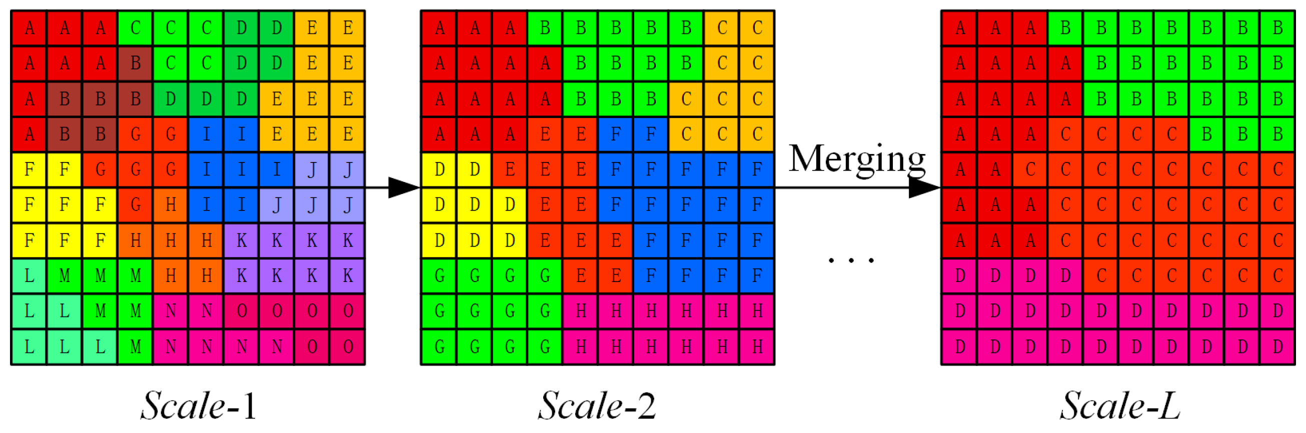
In the proposed method, the two temporal images are first combined into one image by band stacking. The stacked image is then segmented at an over-segmented scale ($scale\text{-}1$) using FNEA. Finally, the objects at scale-1 are merged into multiple scales (scale-2, …, $scale\text{-}L$) using the spectral and spatial features. This means that the image objects at scale-l are merged by several objects at $scale\text{-}\left(l-1\right)$, based on their heterogeneity; in other words, the image objects at different scales should be organized in a hierarchical manner, as shown in Figure 2. It is supposed that most of the objects at scale 1 are over-segmented, while the merged objects at scale-L are under-segmented. Thus, the optimal image segmentation scale is within the L scales.

(2) The optimal image segmentation scale

The multiple scales described above consist of over-segmented dimensions to under-segmented dimensions based on optimal segmentation scale. The optimal image segmentation scale is defined as the scale that maximizes the intra-segment homogeneity and the inter-segment heterogeneity [46]. The variance average weighted by each object area is used as the global intra-segment homogeneity measure, which is calculated, as shown in Equation (5):

$$V=\frac{{{\displaystyle \sum }}_{i=1}^n{a}_i{v}_i}{{{\displaystyle \sum }}_{i=1}^n{a}_i}$$

(5)

where $a_i$ and $v_i$ represent the area and variance of segment $R_i$. n is the total number of objects of the segmentation map.

The global Moran’s I [46], which is a spatial autocorrelation metric, is used as the inter-segment heterogeneity measure, and is calculated, as shown in Equation (6):

$$MI=\frac{n{{\displaystyle \sum }}_{i=1}^n{{\displaystyle \sum }}_{j=1}^n{w}_{ij}\left(y_i-\overline{y}\right)\left(y_j-\overline{y}\right)}{\left({{\displaystyle \sum }}_{i=1}^n{\left(y_i-\overline{y}\right)}^2\right)\left({{\displaystyle \sum }}_{i\ne j}\sum w_{ij}\right)}$$

(6)

where $w_{ij}$ is the spatial adjacency measure of $R_i$ and $R_j$. If regions $R_i$ and $R_j$ are neighbors, $w_{ij}=1$; otherwise, $w_{ij}=0$. $y_i$ is the mean value of region $R_i$, and $y_j$ is the mean value of region $R_j$. $\overline{y}$ is the mean value of each band of the image. Low Moran’s I values indicate a low degree of spatial autocorrelation and high inter-segment heterogeneity.

The parameter of the image segmentation needs to attain high intra-segment homogeneity and high inter-segment heterogeneity. Both measures are rescaled to the range (0–1) using a normalization formula, as shown in Equation (7):

$$\begin{array}{c}{V}_{norm}=\frac{V-V_{min}}{V_{max}-V_{min}}\\ M{I}_{norm}=\frac{MI-M{I}_{min}}{M{I}_{max}-M{I}_{min}}\end{array}$$

(7)

where $V_{min}$ and $M{I}_{min}$ are the minimum values of the weighted variance and Moran’s I, and $V_{max}$ and $M{I}_{max}$ are the maximum values of the weighted variance and Moran’s I at l scales.

To assign an overall “global score” (GS) to each segmentation scale, the $V_{norm}$ and $M{I}_{norm}$ are combined as the objective function, as shown in Equation (8):

$$\mathrm{GS}=V_{norm}+M{I}_{norm}$$

(8)

For each of the segmentations, the GS values are calculated for all the feature bands. In the proposed method, not only the spectral features, but also the texture features, are utilized to calculate the optimal segmentation scale. The average GS values of all the feature bands are used to identify the best image segmentation scale, where the optimal segmentation scale is identified as the one with the lowest average GS value.

2.2.2. Multi-Scale Object-Based D-S Evidence Theory Fusion and Uncertainty Analysis

The scale is of great significance in image analysis and feature recognition, and a single classifier cannot detect all the kinds of changes that may happen in an image. In order to utilize the multi-scale information and the respective advantages of different classifiers, multi-scale fusion is employed to combine the pixel-based change detection results of multiple classifiers from different scales. According to the heterogeneity, our multi-classifier system exploits the KNN, SVM, and ExT classifiers. The ExT classifier [47] was proposed as a computationally efficient and highly randomized extension of RF. Unlike RF, it does not use tree bagging to generate the training subset for each tree. Instead, the entire training set is used to train all the decision trees in the ensemble. In addition, in the node-splitting step, ExT randomly selects the best feature, along with the corresponding value, to split the node. These two changes cause ExT to be less susceptible to overfitting, and enable it to achieve a better performance [48].

(1) Object-based D-S evidence theory fusion

In order to make full use of the respective advantages of the different classifiers, the D-S evidence theory fusion, which is a mathematical tool for uncertainty modeling and reasoning, is employed [49]. In D-S evidence theory fusion, we suppose that $\mathsf{\Theta }$ is the frame of discernment, and then the power set is denoted by $2^{\Theta }$ and $A\in 2^{\Theta }\to [0,1]$. The basic probability assignment function satisfies $\mathrm{m}(\varnothing )=0$ and ${\displaystyle \sum }_{Aϵ\Theta }m\left(A\right)=1$, where $\varnothing$ is the empty set, $m\left(A\right)$ is the mass function, $\mathrm{and}0<m\left(A\right)<1$.

D-S evidence theory fusion involves combining the different evidence with an orthogonal sum. We suppose that there are k sources, and $m_1$, $m_2$, …$m_k$ are the corresponding probability masses. The probability mass for each class $A\in 2^{\Theta }$ of the different evidence sources is denoted as:

$$\{\begin{array}{c}m\left(A\right)=m_1\oplus m_2\oplus \dots \oplus m_k=\frac{{{\displaystyle \sum }}_{\cap A_j=A}{{\displaystyle \prod }}_{1\le i\le k}{m}_i\left(A_j\right)}{K}\\ K={{\displaystyle \sum }}_{\cap A_j\ne \varnothing }{{\displaystyle \prod }}_{1\le i\le k}{m}_i\left(A_j\right)\end{array}$$

(9)

where $K\in \left[0,1\right]$ represents the normalization factor, which reflects the conflict size of the different evidence sources. If K = 0, the different evidence sources are completely in conflict, and evidence fusion cannot be performed.

In the proposed method, the discernment frame $\mathsf{\Theta }=\left\{C,U\right\}$, where C and U represent the changed and unchanged classes, respectively. In order to utilize the scale information and the respective advantages of the different classifiers, the three base classifiers are used at each segmentation level, so that three evidence sources are generated and combined at each segmentation level.

For each scale level, we let $m_k$ ($k=1,2,3)$ be the evidence obtained from the k-th classifier for object $R_i,i=1,2\dots N$ (where N stands for the number of objects in level $l$), and the evidence $m_k=\left\{P_{kc},P_{ku}\right\}$ is defined as follows:

$$\{\begin{array}{c}{P}_{kc}=\frac{{{\displaystyle \sum }}_{j=1}^n{n}_c^j}{n}\\ P_{ku}=\frac{{{\displaystyle \sum }}_{j=1}^n{n}_u^j}{n}\end{array},k=1,2,3$$

(10)

where $P_{kc}$ and $P_{ku}$ represent the probability of object $R_i$ belonging to C and U in level l, respectively; $n_c^j,$ $n_u^j$, and n are the changed pixels, unchanged pixels and total number of pixels in object $R_i$.

The results of $m_{..}$ are then combined using Equation (11):

$$\{\begin{array}{c}K=P_{1c}\ast P_{2c}\ast P_{3c}+P_{1u}\ast P_{2u}\ast P_{3u}\\ P_c=\left(\frac{1}{K}\right)\ast P_{1c}\ast P_{2c}\ast P_{3c}\\ P_u=\left(\frac{1}{K}\right)\ast P_{1u}\ast P_{2u}\ast P_{3u}\end{array}$$

(11)

(2) Uncertainty analysis

For each scale level $l$, a threshold $T_m$ is set to classify the objects $R_i$ using Equation (12). If the $C{D}_i$ satisfies $P_u>T_m$ or $P_c>T_m$, the current scale l can be seen as the appropriate segmentation scale for the object $R_i$, and object $R_i$ is labeled as a “certain” object. In contrast, if the current scale l is too coarse, then $R_i$ is labeled as an “uncertain” object, which is re-classified by the ensemble system.

$$C{D}_i=\{\begin{array}{c} 0, if{P}_u>T_m\\ 1, if{P}_c>T_m\\ 2, others\end{array}$$

(12)

where $C{D}_i=0,1,2$ indicates that $R_i$ belongs to the unchanged, changed, and uncertain classes, respectively.

2.2.3. Unlabeled Sample Selection

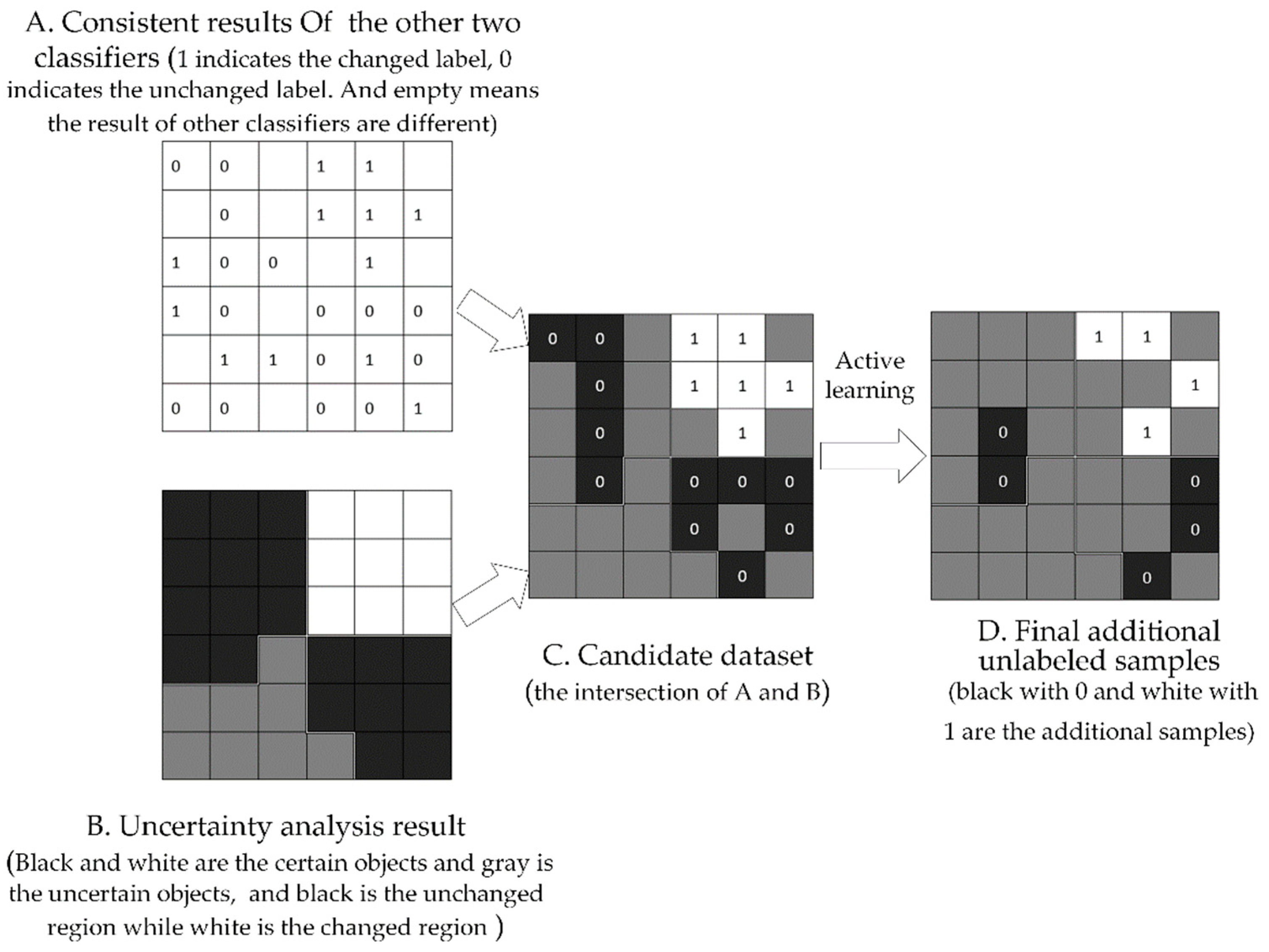
In the standard tri-training algorithm, for a classifier, an unlabeled sample can be labeled when two classifiers obtain the same change detection results. However, the “salt-and-pepper” noise existing in the change detection results, because of the lack of spatial information, can lead to the label that the two classifiers agree on being wrong. Accordingly, in this paper, for a classifier $h_i$, the samples that two classifiers agree on are selected to construct the first candidate set $S_u^1$. The spatial information based on the segmentation objects in each scale is then used to constrain the first candidate and construct the candidate set $S_u$. Finally, the final additional unlabeled samples $S$ are chosen from the candidate set $S_u$ with an AL method based on the breaking ties (BT) algorithm [50], for the training samples of the ensemble system in the next scale layer. The BT algorithm is used to measure the information of the samples by comparing the difference between the maximum probability and sub-probability of posterior probability of samples. The smaller the difference, the more informative the sample and uncertain the samples label is. Therefore, the most informative unlabeled samples are chosen as the final additional samples by BT algorithm in our proposed method.

The detailed process of unlabeled sample selection on each scale is shown in Figure 3.

2.3. The Automatic Change Detection Framework

In the multi-scale uncertainty analysis addressed in Reference [34], a single classifier cannot utilize the advantages of multiple classifiers and the sample selection may lead to the presence of some features with similar spectral information in the training samples, which may not only increase the computational cost, but also affect the performance of the algorithm. Therefore, in order to overcome these shortages, the improved object-based approach for automatic change detection using multiple classifiers and multi-scale uncertainty analysis (OB-MMUA) in high-resolution (HR) remote sensing images is proposed in this study.

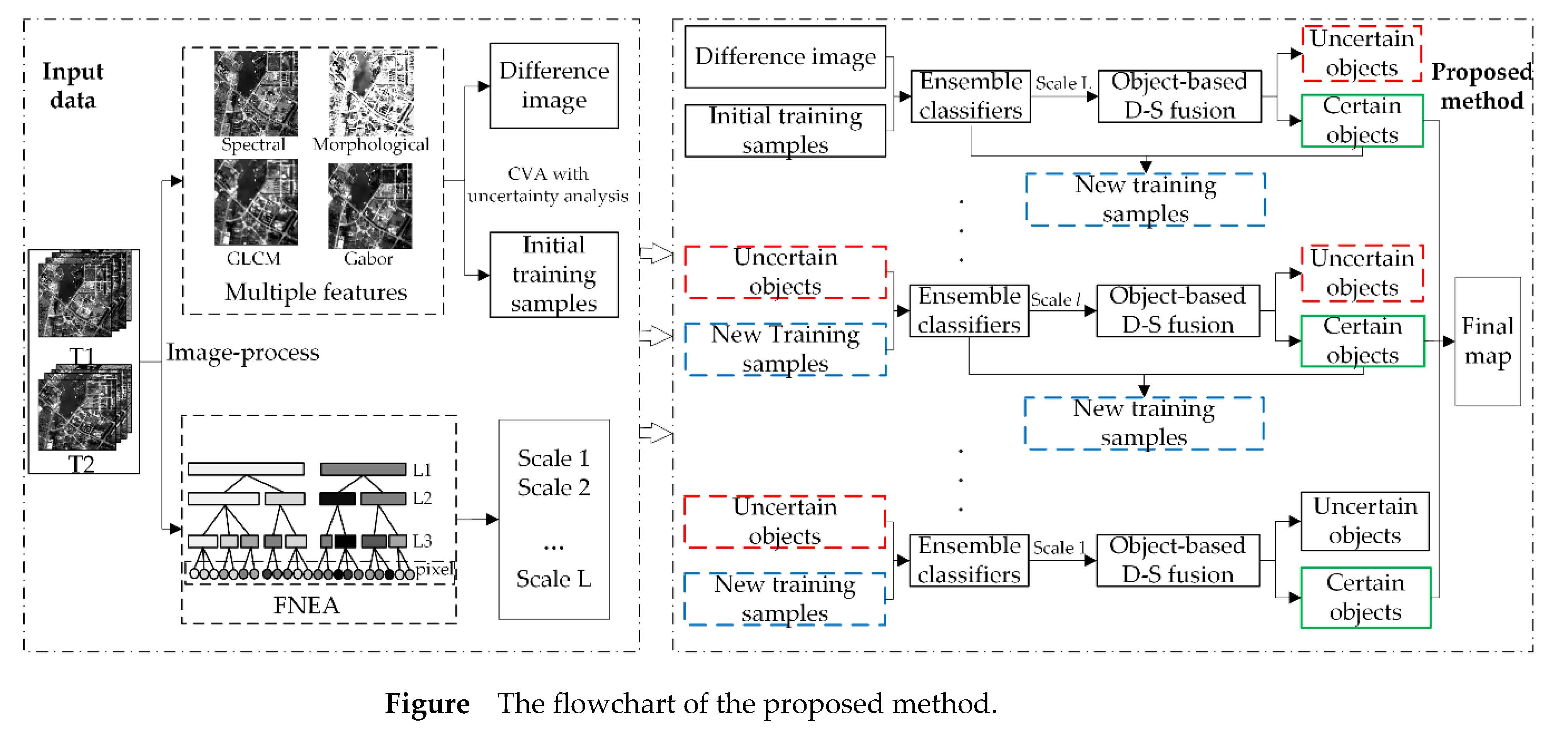
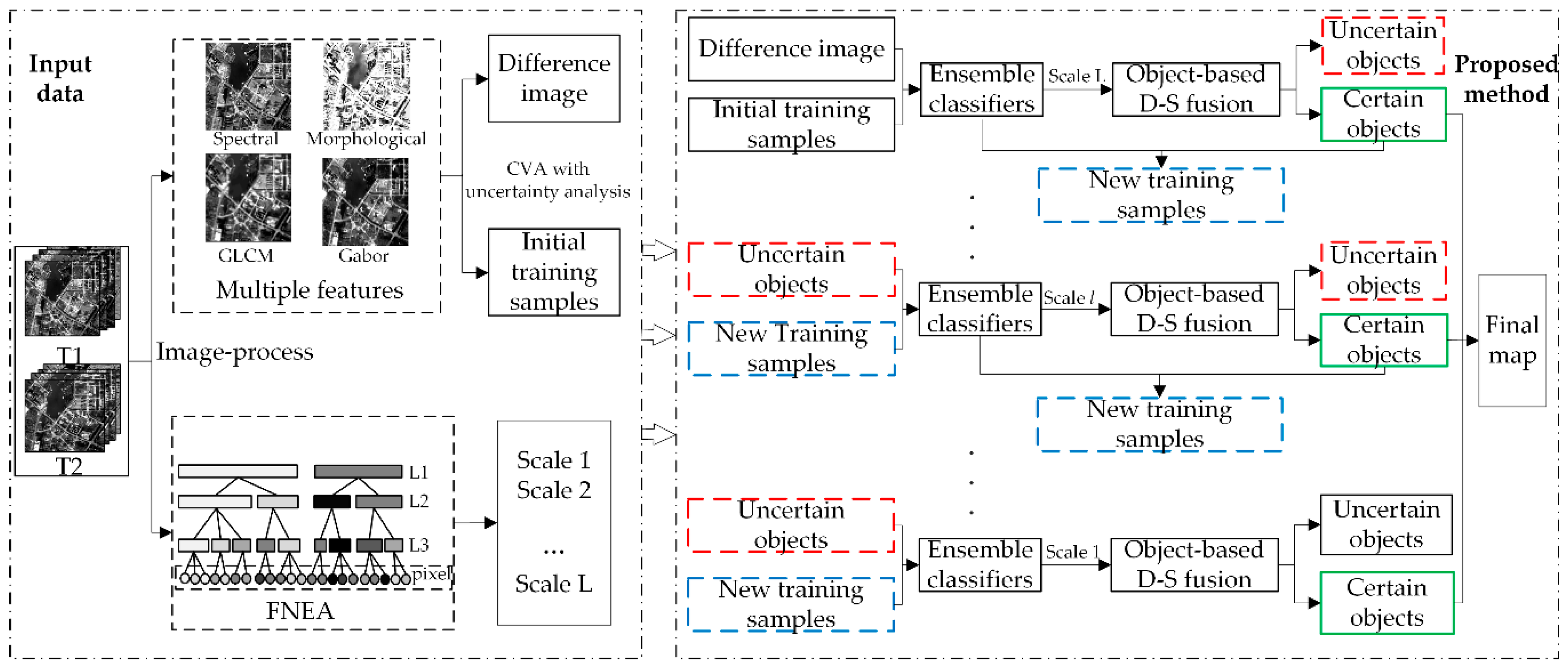
As shown in Figure 4, the experiment mainly includes two parts, one is the construction of multiple features and the formation of multiple scales, and the other part is the proposed change detection method using multiple classifiers and multi-scale uncertainty analysis.

The procedure of the proposed algorithm is summarized as follows.

(1)

Generate a set of segmentation maps ranging from fine scale to coarse scale (scale-1, scale-2, … scale-L) based on optimal image segmentation scale and merging, and obtain the difference image D and initial change detection training samples $S$ with multi-feature change intensity vector and object information (where $y_m$ is the label of initial training samples $x_m$, D is the difference image, and n is the total number of initial training samples);

$$S=(y_m,x_m),x_m\in D,m=1,2,\dots n$$

(2)

Train the classifier $h_i$ with $S$ and obtain the change detection results $C_i \left(i=1,2,3\right)$. Based on the object-based D-S evidence theory fusion and uncertainty analysis in segmentation scale-$l$($l=L, L-1,\dots 1)$, the certain change detection objects $C{D}_c^l$ and uncertain change detection objects $C{D}_u^l$ are obtained;

(3)

For each classifier $h_i$, two candidate sets $S_u^1$ and $S_u^2$ are constructed. $S_u^1$ is composed by the pixels whose neighbors have the same label in $C{D}_c^l$. Pixels that have the same label given by another two classifiers compose $S_u^2.$

(4)

Select samples which have the same label in two candidate sets to construct the third candidate set $S_u^3$, $S_u^3=S_u^1\cap S_u^2\cap \left(!S\right)$;

(5)

Select $S^{\prime }$ based on BT from $S_u^3$ and construct the new training samples $S$ for classifier $h_i$, $S=S\cup S^{\prime }$;

(6)

Train the classifier $h_i$ with the last $S$ and reclassify the uncertain objects $C{D}_u^l$;

(7)

Repeat step (2) ~ (6) in next scale $l$ ($l=l-1$) until all $C{D}_u^l$ are refined to certain objects and get the final change detection map.

3. Results

3.1. Experimental Parameters

In the proposed method, the parameters were set as follows:

• Classifier parameters: $n\_estimators=400$ and $\max \_feature=6$ for the RF classifier; $k=4$ for the KNN classifier; $n\_estimators=600$ and $max\_features=6$ for the ExT classifier; and $\mathrm{c}=0.036,\mathsf{\gamma }=0.25$ and $\mathrm{c}=1.515,\mathsf{\gamma }=16$ for the SVM classifier for the two datasets, respectively, according to the 2-D grid search strategy.
• Scale size: $scale=10,15,20$ for the ZY-3 dataset; and $scale=50,60,70$ for the GF-2 dataset, according to the GS value.
• Uncertainty threshold: The threshold for the uncertainty analysis was set to 0.75 for the two datasets, which was found to perform the best.
• Training set: We chose 500 changed and unchanged samples based on CVA combined with EM as the initial training samples for change detection. The number of the most useful samples $S^{\prime }$ in each scale was set as 500.

3.2. Experimental Results

Figure 5 shows the multi-scale uncertainty analysis results based on the multiple classifiers, where the black, white, and gray areas denote the unchanged, changed, and uncertain classes, respectively. It can be seen that there are many uncertain objects in the coarse scale shown in Figure 5a,d, and there are fewer uncertain objects in the finer scales shown in Figure 5b–e, which confirms the effectiveness of the use of the multi-scale information.

In order to analyze the effectiveness of the proposed OB-MMUA method, we compared it with the supervised pixel-wise change detection methods (S-PWCM) of ELM, MLR, KNN, and SVM; the homogeneous ensemble system methods of RF and ExT; the multiple-classifier system (MCS) based on D-S; the unsupervised pixel-wise change detection method (U-PWCM) based on CVA combined with the EM algorithm; OBCD based on optimal scale (OB-OS); and OBCD using multi-scale fusion (OB-MSF). In this study, all the experiments were implemented in ENVI 5.3 and Python 2.7.

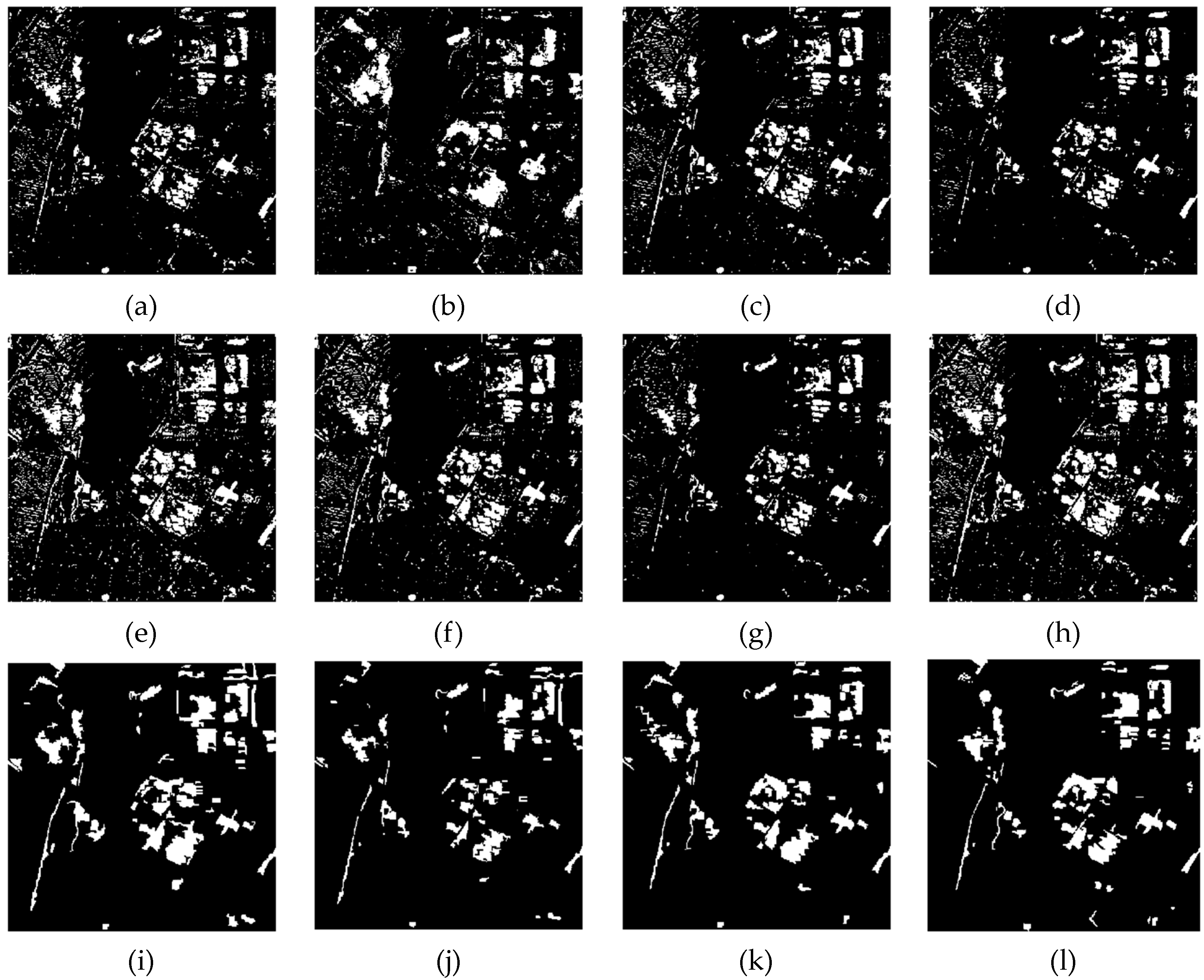
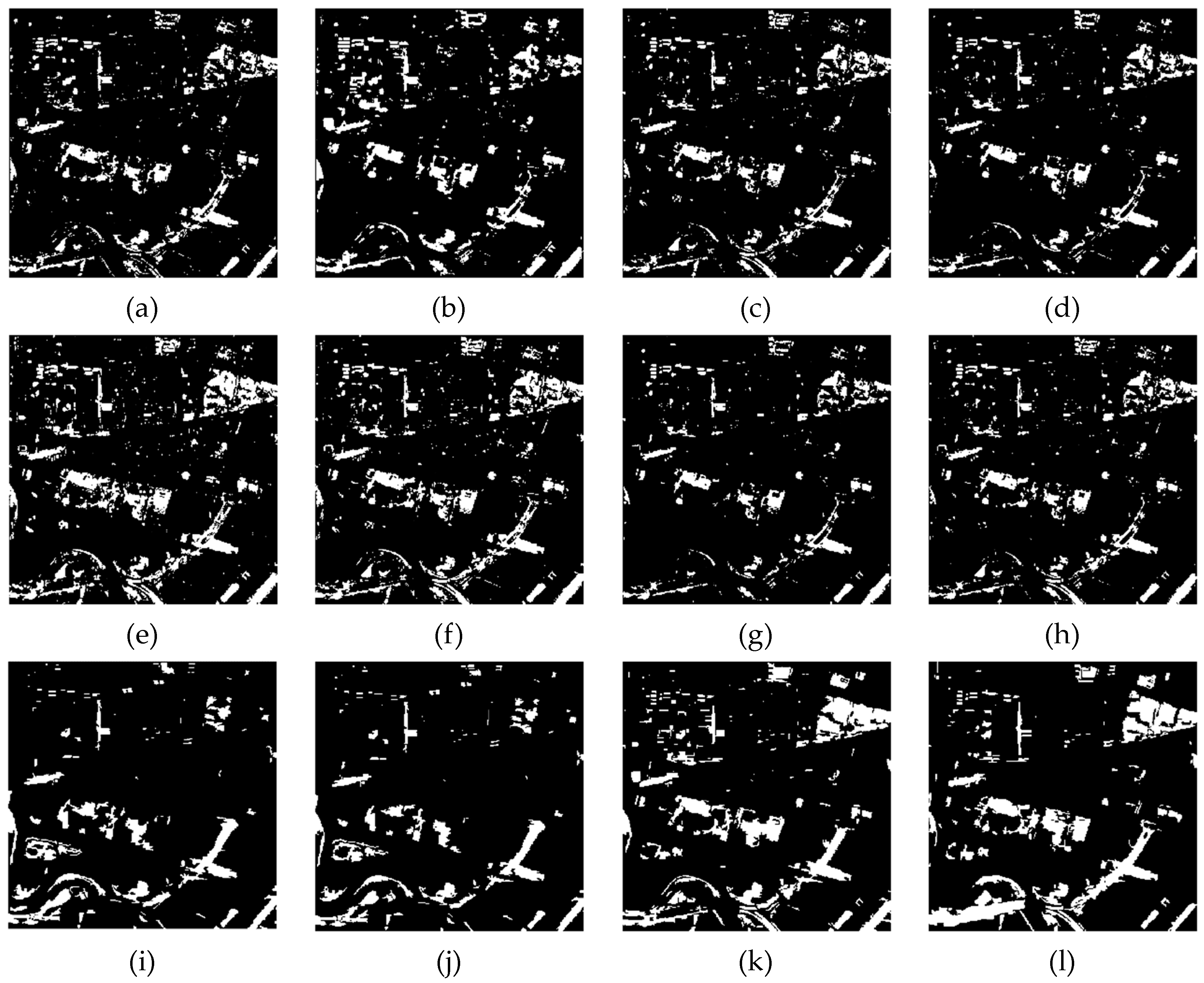
Figure 6 and Figure 7 show the change maps and reference change maps for the two datasets, where the black and white areas denote the unchanged and changed classes, respectively. It can be seen from the results of the change maps that the changed regions in the ZY-3 dataset mainly comprise the change of vegetation and bare land to roads and buildings. The changed regions in the GF-2 dataset mainly comprise the increase of buildings and roads, and the decrease of grassland. Compared with the reference change maps in Figure 6l and Figure 7l, the change detection results of OB-MMUA shown in Figure 6k and Figure 7k are more consistent with the reference change maps. While multi-feature information is utilized, the pixel-wise change detection method still has lots “salt-and-pepper” noise due to the lack using of spatial context, especially in Figure 6a–h. After utilizing the segmented object information constraint, some of the “salt-and-pepper” noise in the change detection result based on OBCD is suppressed, as shown in Figure 6i–l and Figure 7i–l. In OB-MSF, the change detection results from the different scales are treated independently, which neglects the scale constraints between scales and causes a lot of miss-detected pixels (particularly in the upper right of Figure 7i,j). In contrast to OB-MSF, the scale constraints are considered by OB-MMUA, which has fewer missed and false detected pixels. From Figure 6e–f and Figure 7e–f, we can see that the method based on ExT performs better than RF, which demonstrates the improvement of ExT over RF. From Figure 6c,d,f and Figure 7c,d,f, we can see that the change map obtained by SVM contains a lot missed pixels, and the classifiers based on KNN and ExT result in more false detected pixels, which shows the complementarity of these classifiers in vision.

3.3. Anaysis and Discussion

In order to evaluate the performance of the proposed change detection approach quantitatively, four indices were adopted to assess the results by comparing the detection results with the ground reference map: (1) Overall accuracy (OA); (2) Kappa coefficient; (3) commission ratio; and (4) omission ratio, which are defined as:

$$OA=\frac{\left(N_{11}+N_{00}\right)}{(N_{11}+N_{00}+N_{01}+N_{10})}$$

$$Kappa=\frac{N\ast \left(N_{11}+N_{00}\right)-\left((N_{11}+N_{10})\ast \left(N_{11}+N_{01}\right)+\left(N_{01}+N_{00}\right)\ast \left(N_{10}+N_{00}\right)\right)}{N^2-\left((N_{11}+N_{10})\ast \left(N_{11}+N_{01}\right)+\left(N_{01}+N_{00}\right)\ast \left(N_{10}+N_{00}\right)\right)}$$

$$Commissionratio=\frac{N_{01}}{\left(N_{01}+N_{11}\right)}$$

$$Omissionratio=\frac{N_{10}}{\left(N_{10}+N_{00}\right)}$$

where $N_{11}$ and $N_{00}$ are the numbers of changed pixels and unchanged pixels correctly detected, respectively; $N_{10}$ is the number of missed changed pixels; $N_{01}$ is the number of unchanged pixels in the ground reference that are detected as changed in the change map; and N is the total number of pixels of the ground reference.

The accuracies of the change detection for the two datasets are listed in

Table 2. Accuracy of the different change detection methods for the ZY-3 dataset.

Method		OA	Kappa	Commission	Omission
S-PWCM	ELM	0.9387	0.6083	0.3668	0.3495
	MLR	0.9178	0.5251	0.4897	0.3550
	KNN	0.9386	0.6344	0.3853	0.2687
	SVM	0.9511	0.6671	0.2633	0.3448
Ensemble system	RF	0.9173	0.5772	0.4937	0.1973
	ExT	0.9324	0.6255	0.4275	0.2151
	MCS	0.9505	0.6603	0.2629	0.3566
U-PWCM	EM	0.9243	0.6068	0.4665	0.1781
OBCD	OB-OS	0.9267	0.6267	0.4589	0.1362
	OB-MSF	0.9463	0.6283	0.2867	0.3906
	OB-MMUA	0.9698	0.8103	0.1979	0.1470

and

Table 3. Accuracy of the different change detection methods for the GF-2 dataset.

Method		OA	Kappa	Commission	Omission
S-PWCM	ELM	0.9127	0.5960	0.2133	0.4550
	MLR	0.8958	0.5349	0.3184	0.4744
	KNN	0.9192	0.6181	0.1593	0.4550
	SVM	0.9093	0.5597	0.1846	0.5163
Ensemble system	RF	0.9181	0.6577	0.2629	0.3243
	ExT	0.9226	0.6604	0.2121	0.3632
	MCS	0.9074	0.5327	0.1513	0.5608
U-PWCM	EM	0.9160	0.5284	0.1705	0.4716
OBCD	OB-OS	0.8942	0.4977	0.3897	0.5452
	OB-MSF	0.8948	0.4842	0.2623	0.5756
	OB-MMUA	0.9310	0.7164	0.2266	0.2596

. It can be clearly seen that the proposed OB-MMUA obtains a higher change detection accuracy than the other methods. The accuracy of OB-MMUA is the highest among all the methods, with OAs of 0.9698 and 0.9310 for the two datasets. Compared with MCS and OB-MSF, this represents an OA increase of 1.93% and 2.35% for the ZY-3 dataset, and 2.36% and 3.62% for the GF-2 dataset. The Kappa coefficient is increased by 0.15 and 0.18 for the ZY-3 dataset, and by 0.18 and 0.23 for the GF-2 dataset. These results demonstrate the effectiveness and the generalizability of the proposed method.

From the results, it has shown the effectiveness of the proposed method. The significances of the proposed method are shown as follows: (1) Multiple texture features of high-resolution remote sensing images are utilized to make up for the insufficient of spectral information in high-resolution remote sensing imagery; (2) instead of single classifier, multi-classifier ensemble system based on KNN, SVM, and ExT is constructed to obtain the multiple type change information; (3) active learning is used to solve the problem of insufficiency of training samples in supervised change detection methods; and (4) multi-scale segmentation maps are utilized to reduce the dependence of change detection accuracy on segmentation scales.

4. Conclusions

In this paper, an object-based approach for automatic change detection using multiple classifiers and multi-scale uncertainty analysis has been proposed. In the proposed method, macro and micro-texture features are extracted to construct the input data, along with the spectral features. In addition, according to the optimal segmentation scale, multiple scales ranging from fine to coarse are generated by image merging. Three classifiers are then used to construct the optimal classifier ensemble based on the diversity, and unlabeled samples are selected using the AL method combined with the segmented object information. Finally, multi-scale uncertainty analysis is implemented from coarse to fine scales by the multi-classifier ensemble system, and the final change detection map is generated by combining all the “certain” objects in all the scales. To confirm the effectiveness of the proposed method, we conducted experiments using multispectral images collected by the ZY-3 and GF-2 satellites. The experimental results confirmed that the proposed OB-MMUA method performs better than the previous state-of-the-art change detection methods.

However, the new approach still suffers from two major limitations. First, all the features are treated equally and the proposed method lacks the analysis of the weight of different features; second, the proposed method lacks considering the proportion of training samples for changed and unchanged. These questions will be considered in future study.

References

- Du, P.; Liu, S.; Gamba, P.; Tan, K.; Xia, J. Fusion of Difference Images for Change Detection Over Urban Areas. IEEE J. Sel. Top. Appl. Earth Obs. Remote Sens. 2012, 5, 1076–1086. [Google Scholar] [CrossRef]
- Li, H.; Xiao, P.; Feng, X.; Yang, Y.; Wang, L.; Zhang, W.; Wang, X.; Feng, W.; Chang, X. Using land long-term data records to map land cover changes in china over 1981–2010. IEEE J. Sel. Top. Appl. Earth Obs. Remote Sens. 2017, 10, 1372–1389. [Google Scholar] [CrossRef]
- Huang, X.; Zhang, L.; Zhu, T. Building change detection from multitemporal high-resolution remotely sensed images based on a morphological building index. IEEE J. Sel. Top. Appl. Earth Obs. Remote Sens. 2013, 7, 105–115. [Google Scholar] [CrossRef]
- Tang, Y.; Huang, X.; Zhang, L. Fault-Tolerant Building Change Detection from Urban High-Resolution Remote Sensing Imagery. IEEE Geosci. Remote Sens. Lett. 2013, 10, 1060–1064. [Google Scholar] [CrossRef]
- Corresponding, D.L.; Mausel, P.; Brondízio, E.; Moran, E. Change detection techniques. Int. J. Remote Sens. 2004, 25, 2365–2401. [Google Scholar]
- Malmir, M.; Zarkesh, M.M.K.; Monavari, S.M.; Jozi, S.A.; Sharifi, E. Urban development change detection based on multi-temporal satellite images as a fast tracking approach—A case study of Ahwaz county, southwestern Iran. Environ. Monit. Assess. 2015, 187, 4295. [Google Scholar] [CrossRef] [PubMed]
- Zhou, J.; Yu, B.; Qin, J. Multi-level spatial analysis for change detection of urban vegetation at individual tree scale. Remote Sens. 2014, 6, 9086–9103. [Google Scholar] [CrossRef]
- Xiao, P.; Zhang, X.; Wang, D.; Yuan, M.; Feng, X.; Kelly, M. Change detection of built-up land: A framework of combining pixel-based detection and object-based recognition. ISPRS J. Photogramm. Remote Sens. 2016, 119, 402–414. [Google Scholar] [CrossRef]
- Hu, T.; Huang, X.; Li, J.; Zhang, L. A novel co-training approach for urban land cover mapping with unclear Landsat time series imagery. Remote Sens. Environ. 2018, 217, 144–157. [Google Scholar] [CrossRef]
- Azzouzi, S.A.; Vidal, A.; Bentounes, H.A. In Enhancement of the double flexible pace search threshold determination for change vector analysis. Int. Symp. Remote Sens. Environ. 2015, 7, 599–603. [Google Scholar] [CrossRef]
- Song, X.; Bo, C. Change Detection Using Change Vector Analysis from Landsat TM Images in Wuhan. Procedia Environ. Sci. 2011, 11, 238–244. [Google Scholar] [Green Version]
- Moser, G.; Angiati, E.; Serpico, S.B. Multiscale unsupervised change detection by Markov random fields and wavelet transforms. IEEE Geosci. Remote Sens. Lett. 2011, 8, 725–729. [Google Scholar] [CrossRef]
- Huang, G.; Zhu, Q.; Siew, C. In Extreme learning machine: A new learning scheme of feedforward neural networks. IEEE Int. Jt. Conf. Neural Netw. 2004, 982, 985–990. [Google Scholar]
- Volpi, M.; Kanevski, M. Supervised change detection in VHR images using support vector machines and contextual information. Int. J. Appl. Earth Obs. Geoinf. 2010, 20, 77–85. [Google Scholar] [CrossRef]
- Feng, W.; Sui, H.; Tu, J.; Huang, W.; Sun, K. A novel change detection approach based on visual saliency and random forest from multi-temporal high-resolution remote-sensing images. Int. J. Remote Sens. 2018, 39, 7998–8021. [Google Scholar] [CrossRef]
- Guo, G.; Wang, H.; Bell, D.; Bi, Y.; Greer, K. KNN Model-Based Approach in Classification. In On The Move to Meaningful Internet Systems 2003: CoopIS, DOA, and ODBASE; Lecture Notes in Computer Science; Springer: Berlin/Heidelberg, Germany, 2003; Volume 2888, pp. 986–996. [Google Scholar]
- Bachtiar, L.R.; Unsworth, C.P.; Newcomb, R.D.; Crampin, E.J. Multilayer perceptron classification of unknown volatile chemicals from the firing rates of insect olfactory sensory neurons and its application to biosensor design. Neural Comput. 2014, 25, 259–287. [Google Scholar] [CrossRef] [PubMed]
- Wang, Q.; Liu, S.; Chanussot, J.; Li, X. Scene classification with recurrent attention of VHR remote sensing images. IEEE Trans. Geosci. Remote Sens. 2018. [Google Scholar] [CrossRef]
- Wang, Q.; Yuan, Z.; Du, Q.; Li, X. Getnet: A general end-to-end 2-d CNN framework for hyperspectral image change detection. Ieee Trans. Geosci. Remote Sens. 2019, 57, 3–13. [Google Scholar] [CrossRef]
- Li, Y.; Guo, H.; Liu, X.; Li, Y.; Li, J. Adapted ensemble classification algorithm based on multiple classifier system and feature selection for classifying multi-class imbalanced data. Knowl.-Based Syst. 2016, 94, 88–104. [Google Scholar] [CrossRef]
- Tan, K.; Jin, X.; Plaza, A.; Wang, X.; Xiao, L.; Du, P. Automatic change detection in high-resolution remote sensing images by using a multiple classifier system and spectral–spatial features. IEEE J. Sel. Top. Appl. Earth Obs. Remote Sens. 2016, 9, 3439–3451. [Google Scholar] [CrossRef]
- Huang, X.; Hu, T.; Li, J.; Wang, Q. Mapping Urban Areas in China Using Multisource Data with a Novel Ensemble SVM Method. IEEE Trans. Geosci. Remote Sens. 2018, 56, 4258–4273. [Google Scholar] [CrossRef]
- Du, P.; Xia, J.; Zhang, W.; Tan, K.; Liu, Y.; Liu, S. Multiple classifier system for remote sensing image classification: A review. Sensors 2012, 12, 4764–4792. [Google Scholar] [CrossRef] [PubMed]
- Zhang, H.; Gong, M.; Zhang, P.; Su, L.; Shi, J. Feature-level change detection using deep representation and feature change analysis for multispectral imagery. IEEE Geosci. Remote Sens. Lett. 2017, 13, 1666–1670. [Google Scholar] [CrossRef]
- Huo, C.; Zhou, Z.; Lu, H.; Pan, C.; Chen, K. Fast object-level change detection for VHR images. IEEE Geosci. Remote Sens. Lett. 2010, 7, 118–122. [Google Scholar] [CrossRef]
- Chen, Q.; Chen, Y. Multi-feature object-based change detection using self-adaptive weight change vector analysis. Remote Sens. 2016, 8, 549. [Google Scholar] [CrossRef]
- Huang, X.; Wen, D.; Li, J.; Qin, R. Multi-level monitoring of subtle urban changes for the megacities of china using high-resolution multi-view satellite imagery. Remote Sens. Environ. 2017, 196, 56–75. [Google Scholar] [CrossRef]
- Wang, X.; Liu, S.; Du, P.; Liang, H.; Xia, J.; Li, Y. Object-based change detection in urban areas from high spatial resolution images based on multiple features and ensemble learning. Remote Sens. 2018, 10, 276. [Google Scholar] [CrossRef]
- Tang, Y.; Zhang, L.; Huang, X. Object-oriented change detection based on the Kolmogorov–Smirnov test using high-resolution multispectral imagery. Int. J. Remote Sens. 2011, 32, 5719–5740. [Google Scholar] [CrossRef]
- Peng, D.; Zhang, Y. Object-based change detection from satellite imagery by segmentation optimization and multi-features fusion. Int. J. Remote Sens. 2017, 38, 3886–3905. [Google Scholar] [CrossRef]
- Hao, M.; Shi, W.; Deng, K.; Zhang, H.; He, P. An Object-Based Change Detection Approach Using Uncertainty Analysis for VHR Images. J. Sens. 2016, 2016, 9078364. [Google Scholar] [CrossRef]
- Cao, G.; Li, Y.; Liu, Y.; Shang, Y. Automatic change detection in high-resolution remote-sensing images by means of level set evolution and support vector machine classification. Int. J. Remote Sens. 2014, 35, 6255–6270. [Google Scholar] [CrossRef]
- Tan, K.; Zhang, Y.; Du, Q.; Du, P.; Jin, X.; Li, J. Change Detection based on Stacked Generalization System with Segmentation Constraint. Photogramm. Eng. Remote Sens. 2018, 84, 733–741. [Google Scholar] [CrossRef]
- Zhang, Y.; Peng, D.; Huang, X. Object-based change detection for vhr images based on multiscale uncertainty analysis. IEEE Geosci. Remote Sens. Lett. 2018, 15, 13–17. [Google Scholar] [CrossRef]
- Kuncheva, L.I.; Whitaker, C.J. Measures of diversity in classifier ensembles and their relationship with the ensemble accuracy. Mach. Learn. 2003, 51, 181–207. [Google Scholar] [CrossRef]
- Lu, Q.; Ma, Y.; Xia, G. Active learning for training sample selection in remote sensing image classification using spatial information. Remote Sens. Lett. 2017, 8, 1211–1220. [Google Scholar] [CrossRef]
- Du, P.; Zhao, Y.; Liu, S. Information fusion techniques for change detection from multi-temporal remote sensing images. Inf. Fusion 2013, 14, 19–27. [Google Scholar] [CrossRef]
- Li, Q.; Huang, X.; Wen, D.; Liu, H. Integrating multiple textural features for remote sensing image change detection. Photogramm. Eng. Remote Sens. 2017, 83, 109–121. [Google Scholar] [CrossRef]
- Chandy, D.; Johnson, J.; Selvan, S. Texture feature extraction using gray level statistical matrix for content-based mammogram retrieval. Multimed. Tools Appl. 2014, 72, 2011–2024. [Google Scholar] [CrossRef]
- Mura, M.D.; Benediktsson, J.A.; Bovolo, F.; Bruzzone, L. An unsupervised technique based on morphological filters for change detection in very high resolution images. IEEE Geosci. Remote Sens. Lett. 2008, 5, 433–437. [Google Scholar] [CrossRef]
- Li, Z.; Shi, W.; Zhang, H.; Hao, M. Change detection based on Gabor wavelet features for very high resolution remote sensing images. IEEE Geosci. Remote Sens. Lett. 2017, 14, 783–787. [Google Scholar] [CrossRef]
- Menze, B.H.; Kelm, M.B.; Masuch, R.; Himmelreich, U.; Bachert, P.; Petrich, W.; Hamprecht, F.A. A comparison of random forest and its Gini importance with standard chemometric methods for the feature selection and classification of spectral data. BMC Bioinform. 2009, 10, 213. [Google Scholar] [CrossRef] [PubMed]
- Bruzzone, L.; Prieto, D.F. Automatic analysis of the difference image for unsupervised change detection. IEEE Trans. Geosci. Remote Sens. 2000, 38, 1171–1182. [Google Scholar] [CrossRef]
- Hay, G.J.; Blaschke, T.; Marceau, D.J.; Bouchard, A. A comparison of three image-object methods for the multiscale analysis of landscape structure. ISPRS J. Photogramm. Remote Sens. 2003, 57, 327–345. [Google Scholar] [CrossRef]
- Zhang, X.; Du, S. Learning selfhood scales for urban land cover mapping with very-high-resolution satellite images. Remote Sens. Environ. 2016, 178, 172–190. [Google Scholar] [CrossRef]
- Espindola, G.M.; Camara, G.; Reis, I.A.; Bins, L.S.; Monteiro, A.M. Parameter selection for region-growing image segmentation algorithms using spatial autocorrelation. Int. J. Remote Sens. 2006, 27, 3035–3040. [Google Scholar] [CrossRef]
- Geurts, P.; Ernst, D.; Wehenkel, L. Extremely randomized trees. Mach. Learn. 2006, 63, 3–42. [Google Scholar] [CrossRef] [Green Version]
- John, V.; Liu, Z.; Guo, C.; Mita, S.; Kidono, K. In Real-time lane estimation using deep features and extra trees regression. Pac.-Rim Symp. Image Video Technol. 2016, 9431, 721–733. [Google Scholar]
- Shi, A.; Gao, G.; Shen, S. Change detection of bitemporal multispectral images based on FCM and D-S theory. EURASIP J. Adv. Signal Process. 2016, 1, 96–107. [Google Scholar] [CrossRef]
- Tan, K.; Zhu, J.; Du, Q.; Wu, L.; Du, P. A novel tri-training technique for semi-supervised classification of hyperspectral images based on diversity measurement. Remote Sens. 2016, 8, 749. [Google Scholar] [CrossRef]
Figure 1.
True-color images and reference change maps of the two datasets. (a,b) True-color images acquired by ZY-3, (c) Reference change map of the ZY-3 dataset, (d,e) True-color images acquired by GF-2, (f) Reference change map of the GF-2 dataset.
Figure 2.
Flowchart of image merging.
Figure 3.
The process of unlabeled sample selection on one scale.
Figure 4.
The flowchart of the proposed method.
Figure 5.
Change detection results from the different scales. (a–c) The change detection results from scales 20, 15, and 10, respectively, for the ZY-3 dataset. (d–f) The change detection results from scales 70, 60, and 50, respectively, for the GF-2 dataset.
Figure 6.
Change detection maps obtained for the ZY-3 dataset by: (a) ELM, (b) MLR, (c) KNN, (d) SVM, (e) RF, (f) ExT, (g) MCS, (h) EM, (i) OB-OS, (j) OB-MSF, and (k) OB-MMUA. (l) Reference map.
Figure 7.
Change detection maps obtained for the GF-2 dataset by: (a) ELM, (b) MLR, (c) KNN, (d) SVM, (e) RF, (f) ExT, (g) MCS, (h) EM, (i) OB-OS, (j) OB-MSF, and (k) OB-MMUA. (l) Reference map.