Effects of Growth Stage Development on Paddy Rice Leaf Area Index Prediction Models


1
College of Natural Resources and Environment, Northwest A&F University, Yangling 712100, Shaanxi, China
2
School of Geography and Planning, Sun Yat-sen University, Guangzhou 510275, Guangdong, China
*
Author to whom correspondence should be addressed.
Remote Sens. 2019, 11(3), 361; https://0-doi-org.brum.beds.ac.uk/10.3390/rs11030361
Submission received: 10 January 2019
/
Revised: 30 January 2019
/
Accepted: 8 February 2019
/
Published: 11 February 2019
(This article belongs to the Special Issue Leaf Area Index (LAI) Retrieval using Remote Sensing)
Abstract
:A in situ hyperspectral dataset containing multiple growth stages over multiple growing seasons was used to build paddy rice leaf area index (LAI) estimation models with a special focus on the effects of paddy rice growth stage development. The univariate regression method applied to the vegetation index (VI), the traditional multivariate calibration method of partial least squares regression (PLSR), and modern machine learning methods such as support vector regression (SVR), random forests (RF), and artificial neural networks (ANN) based on the original and first-derivative hyperspectral data were evaluated in this study for paddy rice LAI estimation. All the models were built on the whole growing season and on each separate vegetative, reproductive and ripening growth stage of paddy rice separately. To ensure a fair comparison, the models of the whole growing season were also validated on data for each separate growth stage of the standalone validation dataset. Moreover, the optimal band pairs for calculating narrowband difference vegetative index (DVI), normalized difference vegetation index (NDVI) and simple ratio vegetation index (SR) were determined for the whole growing season and for each separate growth stage separately. The results showed that for both the whole growing season and for each single growth stage, the red-edge and near-infrared band pairs are optimal for formulating the narrowband DVI, NDVI and SR. Among the four multivariate calibration methods, SVR and RF yielded more accurate results than the other two methods. The SVR and RF models built on first-derivative spectra provided more accurate results than the corresponding models on the original spectra for both whole growing season models and separate growth stage models. Comparing the prediction accuracy based on the whole growing season revealed that the RF and SVR models showed an advantage over the VI models. However, comparing the prediction accuracy based on each growth stage separately showed that the VI models provided more accurate results for the vegetative growth stages. The SVR and RF models provided more accurate results for the ripening growth stage. However, the whole growing season RF model on first-derivative spectra could provide reasonable accuracy for each single growth stage.
1. Introduction
Leaf area index (LAI), which is defined as half of the all-sided green leaf area per unit ground area [1], is a key biophysical parameter that reflects biochemical and physiological processes of plants. LAI mapping is important for a wide range of agricultural studies such as stress evaluation [2,3,4], growth status monitoring, and yield estimation [5,6,7]. Remote sensing is a prevalent technique that can provide cost-effective and nondestructive LAI estimation both at regional and global scales. Hyperspectral remote sensing, which is done with narrower spectra bands, allows for characterizing vegetation with a considerably greater amount of information than traditional multispectral techniques [8]. Studies have suggested that hyperspectral data may improve LAI estimation accuracy [9,10,11,12,13].
There are two main approaches to build LAI estimation models from remote sensing data; the empirical statistical approach and the radiative transform model (RTM) approach [8]. The former approach includes univariate regression models built on a vegetation index (VI) and multivariate-calibration-based models using the full reflectance spectrum [14,15,16]. These multivariate calibration techniques include the partial least squares regression (PLSR) methods and modern machine learning methods such as support vector regression (SVR), random forests (RF), and artificial neural networks (ANN). The latter approach generally combines an RTM with different inversion techniques. The RTM approach suffers from ill-posed problems and high computational cost. Furthermore, the accuracy of the RTM inversion results are highly reliant on the realism of the RTM simulation and appropriate RTM parameter initialization [8,17,18].
Vegetation indexes (VIs) are designed to enhance the vegetation signal by simply combining two or few more bands of measured spectra response. The VI method is preferred to the RTM approach and other empirical statistical methods because it is easy to design and parameterize. New possibilities have opened up with the advent of hyperspectral data. The established index formulations such as normalized difference vegetation index (NDVI) [19], simple ratio vegetation index (SR) [20] and difference vegetative index (DVI) [21] computed from specific optimization narrow bands could improve the accuracy of LAI estimations [22,23,24,25]. Hansen et al. [22] showed that red-edge bands are important for building narrowband VI-LAI estimation models by studying field-collected multiple growth stages and cultivars data of winter wheat. Moreover, they concluded that narrowband VI-LAI relationships are optimal and cannot be significantly improved (in wheat crops) by the PLSR method using all hyperspectral bands. Zhao et al. [23] reported that calculating with 690–710 nm and 750–900 nm bands provides better LAI estimation accuracy for cotton canopy, the red band of which is not consistent with the common broadband red channel centers (640–660 nm) onboard the current generation of earth-orbiting satellites. Delegido et al. [24] demonstrated that exhibited the highest linear relationship with the LAI of nine crop types (without paddy rice). Tanaka et al. [25] showed that difference between reflectance values at 760 nm and 739 nm showed outstanding performance for winter wheat LAI assessments. Although the excellent performance of narrowband VIs has been widely demonstrated, how the growth stage development of crops affects the optimal band combinations for the narrowband VIs and its performance has not been fully evaluated.
Univariate regression models based on VIs, which typically use two to three bands, are considered to be too simple for capturing the intrinsic relationships between the observed remote sensing data (particularly hyperspectral data) and the biochemical or biophysical parameters of interest. These models also lack the ability to parameterize spatiotemporal variability [26]. PLSR has been considered to be a powerful alternative to univariate methods and provides better performance in most cases [27,28,29], although there is a study that reported the opposite results [22]. Moreover, the potential performance of the state-of-the-art machine learning methods, such as SVR, RF and ANN, has been explored in several studies [14,15,30]. These studies showed that the state-of-the-art machine learning techniques appear to be more efficient than the VI and PLSR methods in most LAI estimation cases. Furthermore, several studies [14,15] also point out that performance of PLSR and machine learning method is affect by the development of growth stage. Kiala et al. [14] built SVR and PLSR models at different growth stages (early, mid, late and combined) of tropical grassland for LAI estimation. Their results showed that the SVR model yielded better accuracy at the mid-growth stage and whole growing season, whereas the PLSR models performed better at the early and late growth stages. Yuan et al. [15] used PLSR and three machine learning methods (RF, ANN and SVR) to predict soybean LAI over a single growth stage (full pod period) and the whole growing season, and their results showed that the RF model was more accurate for the whole growing season, whereas the ANN model was more suitable for the single growth stage. Whether this pattern also exists in other plants, such as paddy rice, has not been fully explored.
Paddy rice is one of the main crops in the world. Accurately monitoring its growing status will benefit the guidance of its management. Thus, based on a field-collected multiple growth stages over multiple growing seasons canopy reflectance and LAI dataset of paddy rice, this study assessed the performance of VIs, PLSR and three machine learning techniques—SVR, RF and ANN—in estimating paddy rice LAI with a special focus on the effects of growth stage development.
2. Materials and Methods
2.1. Study Area and Experimental Setup
The study was conducted during the 2014–2017 growing seasons (from May to October) on a farmland located in the Ningxia Yellow River irrigation region, China (38°7′25″ N, 106°11′35″ E). This region is characterized by a temperate continental semiarid climate. The average annual precipitation and average annual accumulative temperature are nm and °C [31], respectively. The paddy rice variety Ningjing NO. 37 was used as the test material. The paddy rice was sown in a nursery bed in late April and was transplanted in late May for all four growing seasons.
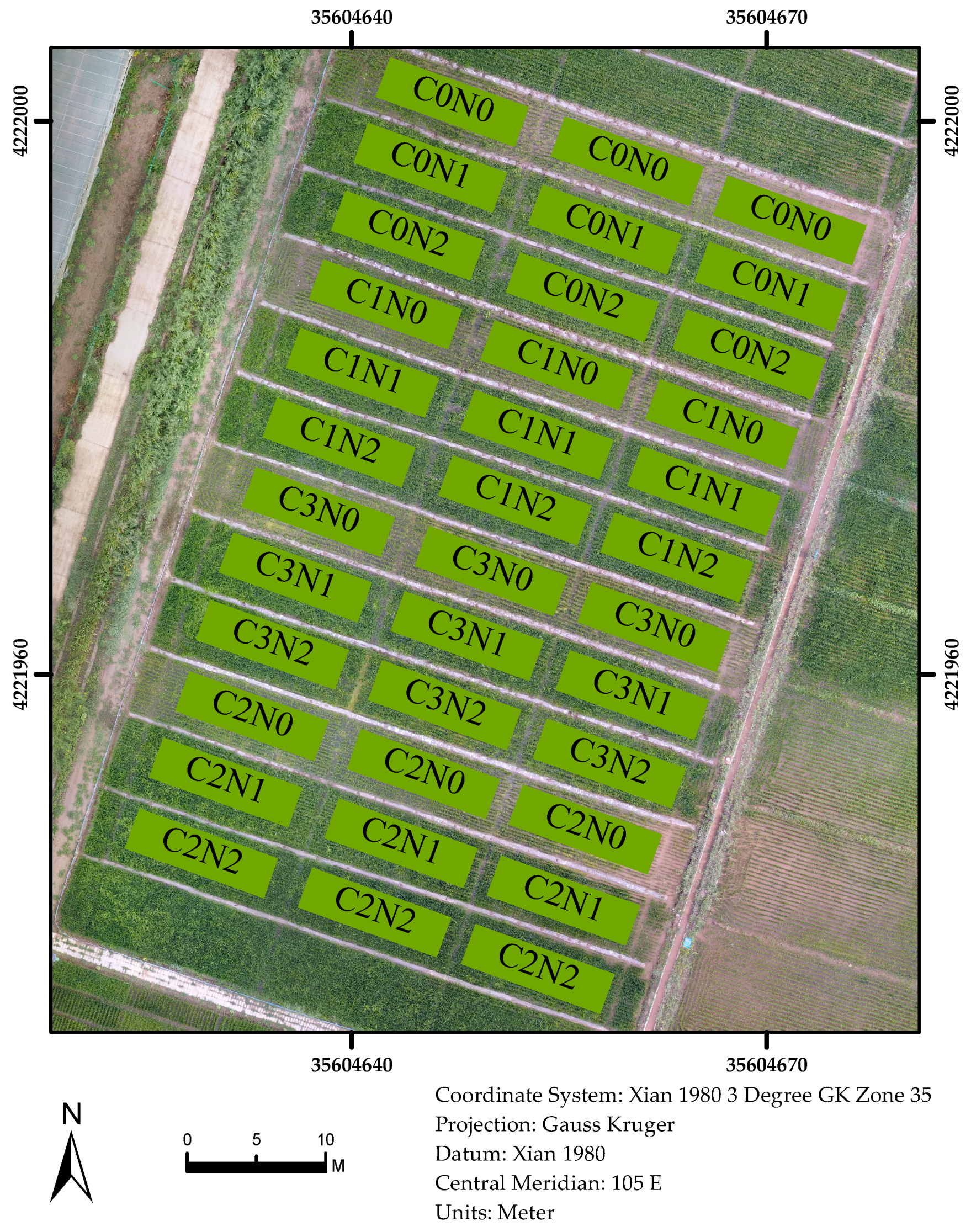
To acquire the necessary reference observations, paddy rice fields with different biochar and nitrogen treatments were used to conduct the field data collection campaigns (detailed in Figure 1). Three nitrogen fertilizer levels (N0 is no fertilizer, N1 is 240 /, and N2 is 300 /) and four biochar levels (C0 is no biochar, C1 is 4500 /, C2 is 9000 /, and C3 is 13,500 /) were applied. The phosphates and potash fertilizers were applied for each plot at recommended levels for this region [31], which were PO 90 / and KO 90 /. The biochar was produced by pyrolysis of wheat straw at 350–550 by the Sanli New Energy Company, Henan Province, China. The biochar had C, N, P and K contents of 65.7%, 0.49%, 0.1% and 1.6%, respectively [31]. Fertilizers and biochar were broadcast on the soil surface and incorporated into the soil by plowing to a depth of approximately 13 cm. Each plot was 14 by 5 . Different treatments were separated by plastic film to 130 cm in depth, preventing water interchange.
2.2. Field Data Collection
Canopy reflectance was measured with an SVC HR1024i spectroradiometer with an 8° field-of-view lens. The spectroradiometer has 1024 channels ranging from 350 nm to 2500 nm. In each plot, canopy reflectance was measured at three randomly selected sample points. Five measurements were conducted at each sample point. The fifteen measurements were averaged to represent the canopy reflectance of the plot. During the measurement, the spectroradiometer was mounted on a tripod and fixed at 1 m above the canopy. All measurements were collected under cloudless weather conditions between 11 am and 2 pm at local time near solar noon. A 2nd-order Savitzky–Golay filter [32] was used to filter the sensor noise, and then the reflectance data were resampled to a spectra resolution of 10 nm. The bands beyond 2400 nm were omitted because of the low signal-to-noise ratio. LAI was measured on the same day with a SunScan Canopy Analysis System. For each plot, two sample points were selected randomly. For each sample point, measurements were taken every 45, starting from the across-ridge direction. The eight measurements were averaged to represent the LAI of the plot.
Data collection campaigns were planned to be conducted one time at each of the vegetative, reproductive and ripening growth stages of paddy rice during the 2014–2017 growing seasons. The specific dates (in form of day after transplantation, DAT) upon which data collection campaigns were conducted are summarized in Table 1. The growth stage was determined according to the rules described by [33].
2.3. Methods
Theoretically, there should have been samples. However, the spectra data of nine plots were missing because of a spectroradiometer failure during the 2016 vegetative growth stage data collection campaign, and another four samples were omitted because of invalid spectral data. Thus, 419 valid data samples were further analyzed. All single growth stage models were calibrated on the corresponding growth stage data of the 2014–2016 growing seasons and validated on the corresponding growth stage data of the 2017 growing season. For the whole growing season models, they were calibrated on the whole growing season data of the 2014–2016 seasons and validated in two different ways. For the first way, the whole growing season models were validated by the whole data of the 2017 growing season. For the second way, the whole growing season models were validated on each separate growth stage data of the 2017 growing season separately. Thus, in this way, a whole growing season model has one specific validation result for each single growth. Therefore, a fair performance comparison could be made between whole growing season models and single growth stage models.
Ten selected VIs were used to predict paddy rice LAI separately with nonlinear regression techniques. Additionally, four multivariate calibration techniques were evaluated, namely, PLSR, SVR, RF and ANN, on the original reflectance and its first-derivative as predictors separately. Both original reflectance and first-derivative spectra were normalized by subtracting the mean and dividing by the standard deviation before model calibration. No feature selection procedure was used to reduce the spectra dimensions. All the VI models were built on the original resolution spectra, whereas the multivariate calibration models were built on the 10 nm resolution spectra.
All models were built in the R environment [34]. The PLSR, RF and SVR models were built using the R packages ‘pls’ [35], ‘randomForest’ [36], and ‘kernlab’ [37], respectively, and the ANN model was built with the R package ‘keras’ [38] with a TensorFlow backend [39].
2.3.1. Vegetation Indices
Ten VIs that have been widely used for LAI estimation were evaluated (Table 2). DVI [21], NDVI [19] and SR [20] were selected because they are the earliest and simplest VIs, and their narrowband versions have great potential to improve the LAI estimation accuracy. The modified soil adjust vegetation index (MSAVI) [40] and enhanced vegetation index (EVI) [41] were used to represent the soil-line-adjusted VIs. The wide dynamic range vegetation index (WDRVI) [42] was developed to linearize the relationship between LAI and NDVI by using weighted coefficients. [16] is a newly developed index that takes advantage of the narrowband information of 705 nm and 750 nm. The MERIS (Medium Resolution Imaging Spectrometer) terrestial chlorophyll index (MTCI) [43], red-edge position (lp) [23] and reflectance at red-edge position (Rp) [23] are VIs that characterize the red-edge information.
First, the optimal narrowband combinations for DVI, NDVI and SR were separately determined for each individual growth stage and for the whole growing season. The indices were calculated by taking all possible two-band pairs and were regressed against LAI on a corresponding calibration dataset. The band pairs that yielded the highest were selected as the optimal bands to formulate the corresponding index for predicting paddy rice LAI. Then, the DVI, NDVI and SR with optimal band combinations (denoted as , and ) and the remaining seven indices were used to build separate LAI estimation models for the corresponding growth stages. The relationship between VIs and LAI was fitted with an exponential function. The simplified Bear’s Law (Equation (1)) was used as suggested by previous studies [44]. The parameters and were empirically fitted by the ‘nlsLM’ function in the R package ’minpack’.
2.3.2. Partial Least Squares Regression
PLSR is a bilinear regression method [45]. It performs component projection by successively reducing the original input data to a few independent latent variables () while maximizing covariability to the response variable of interest and then regressing the latent variables against the response variable. The component projection operation reduces the dimensionality and eliminates the multicollinearity of the input data, and reduces noise. The number of controls the model complexity and is determined by a grid search in this study.
2.3.3. Support Vector Regression
SVR, which has its roots in Vapnik–Chervonenkis (VC) theory as a generalization of support vector machines (SVM), is characterized by the use of kernel functions, sparse solutions, and VC control of the margin and the number of support vectors [37,46]. Using an tube, which is an -insensitive region around the objective function, SVR reformulates the optimization problem to minimize a convex -insensitive loss function and finds the flattest tube that contains as many training samples as possible. The objective function was represented by training samples that lie outside the tube’s boundary (support vectors). The complexity of an SVR model is based on the number of support vectors other than the dimension of the input data, and thus, this approach is efficient in high-dimensional space and is still efficient when the number of observations is less than the input dimension. In this study, the -SVR algorithm with a radial basis kernel function (RBF) was used. The kernel parameter of the RBF kernel and regularization parameter C were determined by a grid search. Here, defines how far a training sample can influence, where a large means ‘close’ and a small means ‘far’. C defines the trade-off between the smoothness of the objective function and the maximum deviation allowed. A large C results in selecting more samples as support vectors, and a small C denotes a smooth objective function.
2.3.4. Random Forests
The RF algorithm is based on the decision tree algorithm and bagging method with an additional layer of randomness in the bagging process [47]. The RF algorithm is as follows: first, draw a bootstrap sample times from the original dataset, and each bootstrap sample is used to build a tree; then, grow an unpruned tree for each bootstrap sample, and only randomly selected predictors are used for each tree; finally, perform prediction by aggregating the tree prediction result, where the aggregation strategy is generally the majority of votes for classification and the average for regression. and are the two key parameters that control the performance and complexity of RF models. In this study, was set at 500, as suggested by Breiman [47]. was determined by a grid search.
2.3.5. Artificial Neural Networks
ANNs are fully connected neural nets organized into layers [39,48]. ANNs typically consist of one input layer, zero to multiple hidden layers and one output layer. Every neuron in a layer is connected to every other neuron in the next layer. The output of the j-th neuron in layer can be calculated by Equation (2), where denotes the i-th neuron in layer l, denotes the weight between the i-th neuron in layer l and the j-th neuron in layer , denotes the bias for the j-th neuron in layer , and f denotes the (nonlinear) active function.
In this work, a single-hidden-layer neural network was constructed. The number of neurons in the input layer was set to 205 according to the input feature dimension (205 bands). The number of neurons in the hidden layer was determined by a grid search. A parametric rectified linear unit (Equation (3)) was used as the activation function for the hidden layer, where was learned in the model calibration procedure. A linear function was used as the activation function for the output layer. The weights and bias were initialized by the Glorot normal initializer and regularized by an L1 regularizer. Finally, the ANN model was optimized by the Adam algorithm [49] with a mean square error loss function.
2.3.6. Parameter Optimization and Precision Evaluation
The normalized root mean square error () and coefficient of determination () of model calibration (cross validated) and validation were used to assess and compare the model precision and robustness. The is defined by Equation (4), where y denotes the observed value, denotes the predicted value, and donate the maximum and minimum observed value, respectively. The key parameters ( for PLSR, for SVR, for RF and for ANN) were determined by a grid search with a repeated (5 times) 10-fold cross-validation procedure (CV) on the calibration dataset (Algorithm 1). The parameter (or parameter combination) associated with the lowest was considered optimal. After the key parameters were determined, the final models were calibrated on the full calibration dataset and evaluated on the corresponding standalone validation dataset. For the VI models, the same CV procedure was used to calculate the cross-validated calibration and . The same fold split scheme across different models was used to ensure a fair comparison. The model with the lowest and highest was considered to be optimal.
| Algorithm 1: Model parameter optimization algorithm |
 |
3. Results
3.1. Descriptive Analysis of Measured LAI
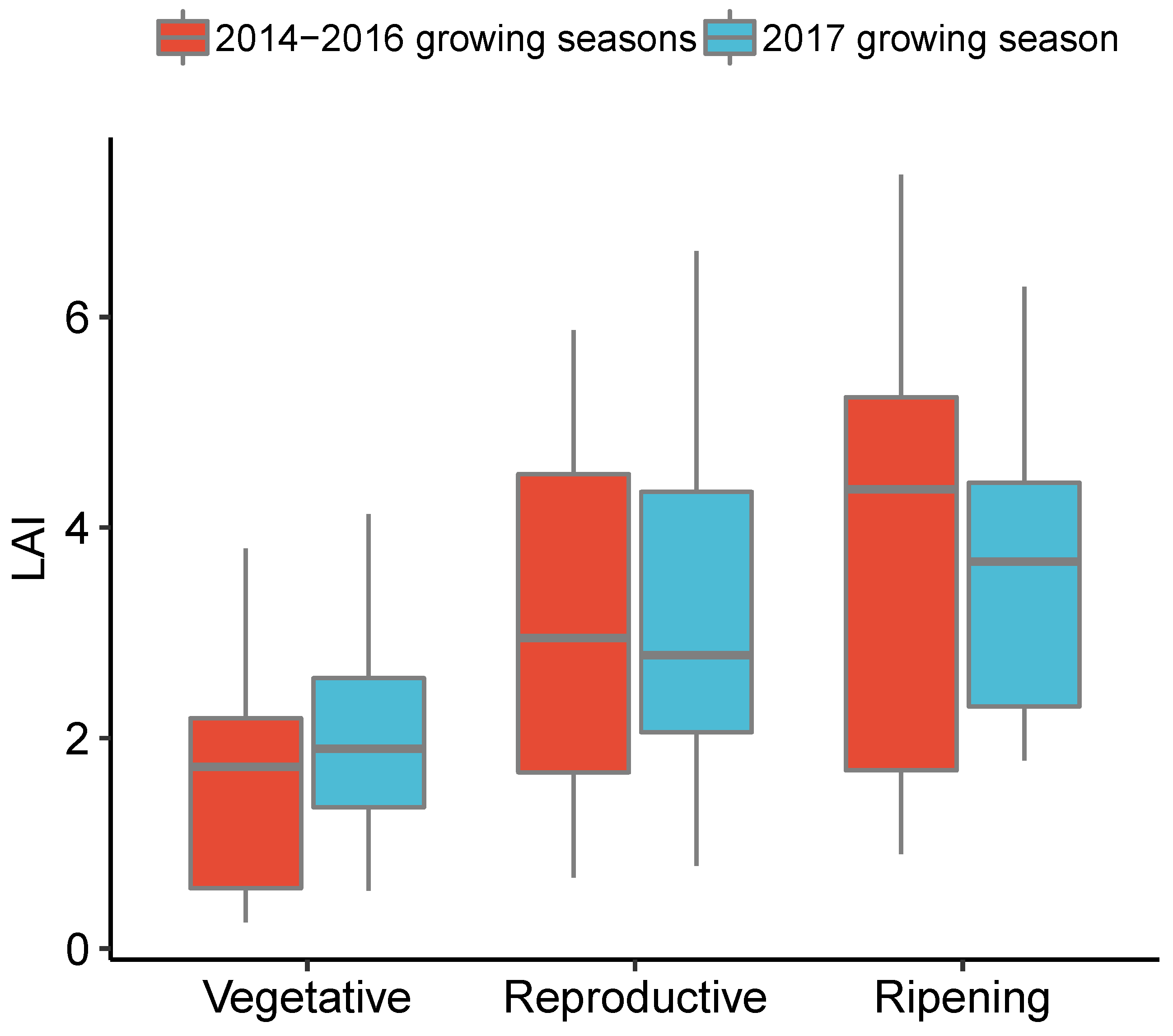
The descriptive statistics for the measured LAI of the whole dataset and each separate growth stage are shown in Table 3. For the whole dataset, LAI ranged between 0.08 and 7.35, with a mean of 2.55 and standard deviation (sd) of 1.63. The measured LAI ranged between 0.08 and 4.12, with a mean of 1.37 and sd of 0.96 for the vegetative growth stage; ranged between 0.65 and 6.62 with a mean of 2.88 and sd of 1.45 for the reproductive growth stage; as well as ranged between 0.72 and 7.36 with a mean of 3.33 and sd of 1.69 for the ripening growth stage. The mean and variance of the measured LAI showed an increasing pattern as the growth stages progressed.
Figure 2 shows the boxplot of the measured LAI. For each single growth stage, the ranges of measured LAI are comparable between the 2014–2016 growing seasons and the 2017 growing season.
3.2. Vegetation Indices
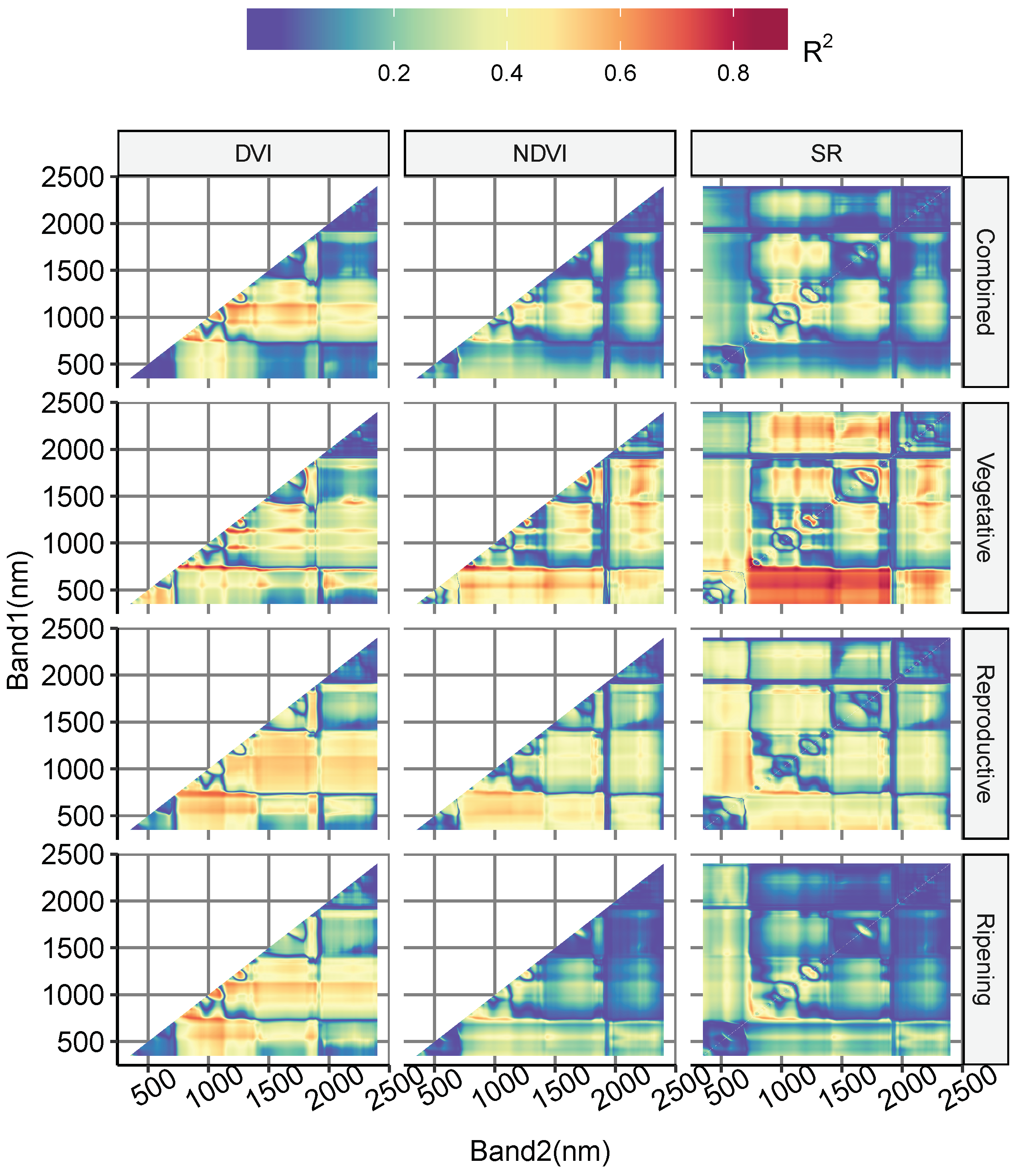
Figure 3 shows the distribution of the calibration between LAI and DVI, NDVI as well as SR taking all possible two-band pairs. The band pairs that yielded a higher were generally with one band in the red-edge region around 750 nm and the other band in the near-infrared (NIR) region, which was around 830 nm for the whole growing season and the vegetative growth stage, around 1130 nm for the reproductive growth stage and around 860 nm for the ripening growth stage. The optimal band pairs for different indices within each specific growth stage and the whole growing season were generally consistent, with slight differences. The band pairs that yielded the highest are summarized in Table 4.
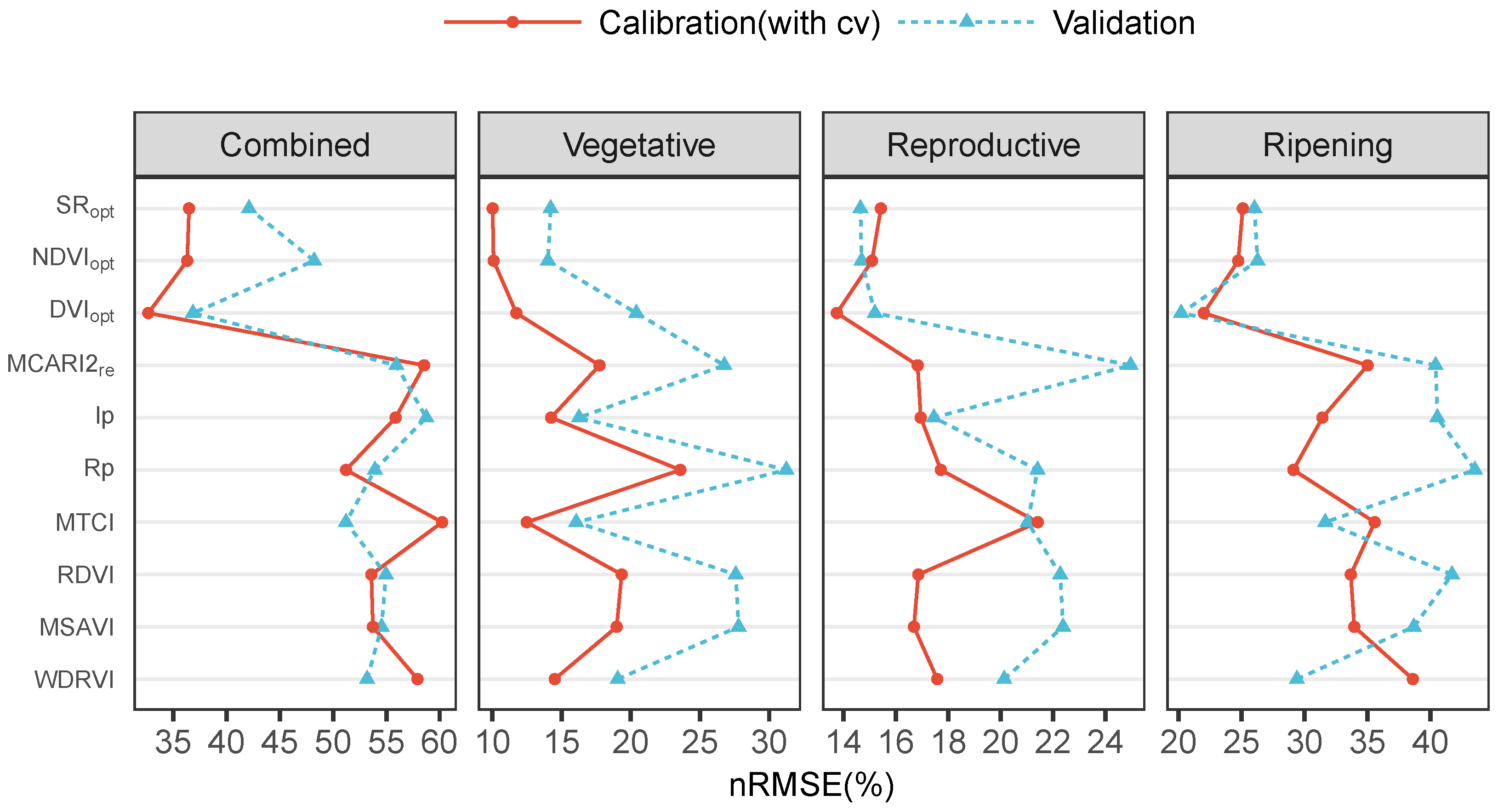
After the optimal band combinations were determined, the corresponding , and and the remaining seven VIs in Table 2 were used to build LAI estimation models for the whole growing season and for each individual growth stage separately. The calibration (with CV) and validation of the ten VIs are shown in Figure 4. The , and all yielded lower both in model calibration and validation than the remaining seven indices. However, there is one exception that, the for vegetative growth stage yielded slightly higher validation . For the whole growing season, the remaining seven VIs yielded more than 50% in both model calibration and validation, which suggested that these VIs are not suitable to predict paddy rice LAI across growth stages. For the single growth stage, the and yielded reasonable accuracy (with less than 20% both for model calibration and validation) at the vegetative and reproductive growth stages but not at the ripening growth stage. The yielded reasonable accuracy at the vegetative growth stage but not at reproductive or ripening growth stages. The remaining four VIs (, , , and ) were always exhibited relatively lower accuracy.
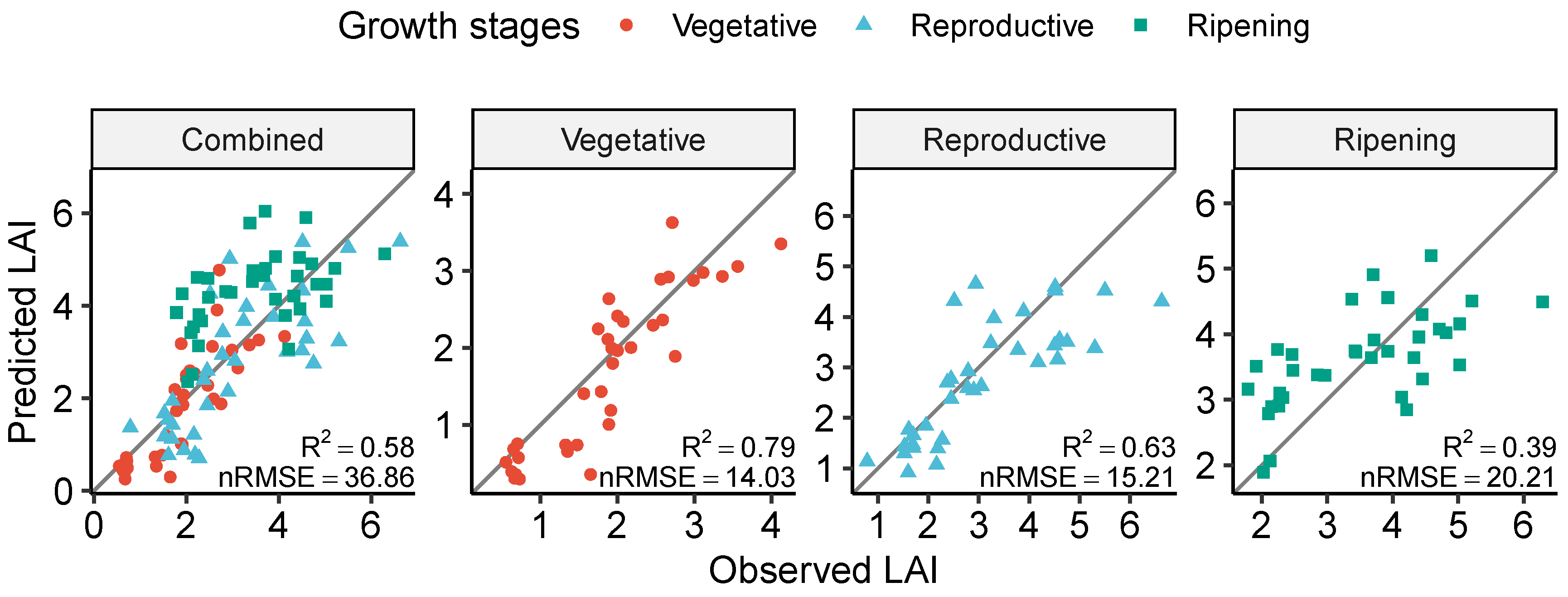
The , , and have the top performance (with lowest or second lowest both in model calibration and validation) for the whole growing season, vegetative, reproductive, and ripening growth stages, respectively. Table 5 shows the validation and of these four indices. Among them, the model (for the whole growing season) was validated by each separate growth stage data of the 2017 growing season, and the , and (for vegetative, reproductive and ripening growth stage respectively) models were validated by the corresponding growth stage data of the 2017 growing season. Figure 5 shows the relationships between the observed and predicted LAI along the 1:1 line on the standalone validation dataset of these four top-performing VI models. The single growth stage models yielded values of 14.00%, 15.20% and 20.20%, as well as of 0.79, 0.63 and 0.39, for the vegetative, reproductive and ripening growth stages, respectively. The validation was comparable with the corresponding cross-validated calibration value (Figure 4). When the whole growing season model was validated on each single growth stage dataset of the growing season, it yielded values of 18.90%, 17.10% and 29.20%, as well as of 0.67, 0.59 and 0.24, for the vegetative, reproductive and ripening growth stages, respectively. Comparing the validation of the single growth stage models and the validation of the whole growing season model over the corresponding single growth stage data, the decrease ratios were 25.60%, 10.80% and 30.70% for the vegetative, reproductive and ripening growth stages, respectively. For the validation , these ratios were 16.71%, 6.73% and 61.54%, respectively. This result suggested that, for the VI method, building LAI estimation models on separate growth stages could improve the model performance when compared to building the models on the whole growing season.
3.3. Partial Least Squares Regression and Machine Learning Methods
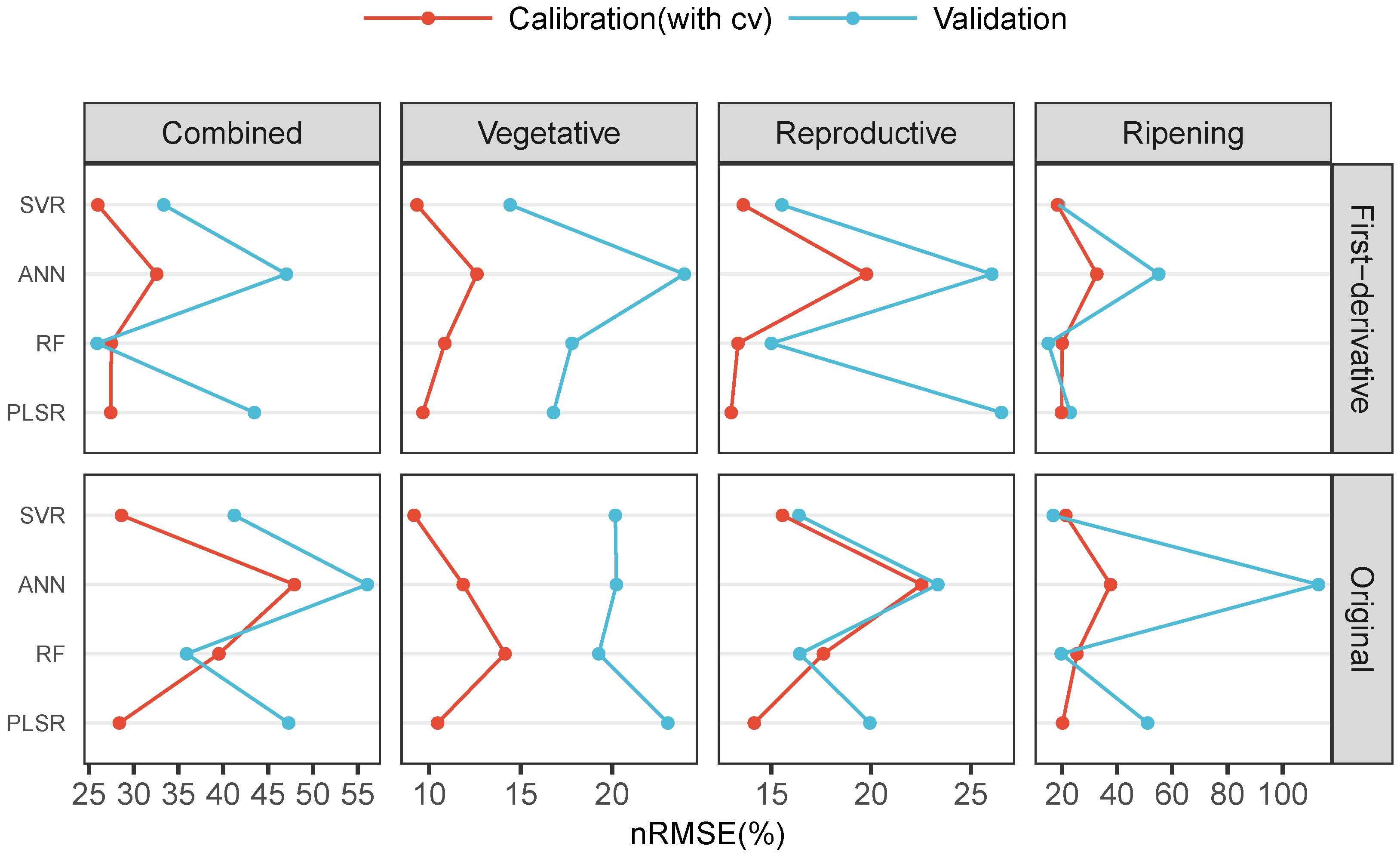
The calibration (with CV) and validation of PLSR and three machine learning methods—RF, ANN and SVR—on the original spectra and first-derivative spectra for the whole growing season and each single growth stage are shown in Figure 6. On both original spectra and first-derivative spectra, the SVR and RF methods clearly showed better performance over the PLSR and ANN methods with lower calibration and validation in most situations. The ANN models had the highest calibration and validation in most situations, which suggested that the ANN methods are suboptimal for building LAI estimation models. The PLSR models showed almost identical calibration with the corresponding SVR models, but they yielded relatively lower validation compared with the corresponding SVR models. This result suggested that the PLSR models were also not robust enough. Thus, the ANN and PLSR methods were not considered for further analysis.
When built on the first-derivative spectra rather than original spectra, the SVR and RF models all showed a decrease in validation for the whole growing season and for each single growth stage. However, there was one exception of the SVR model at the ripening growth stage. The decrease ratios were 27.86%, 7.60%, 8.67% and 23.93% for the RF method of the whole growing season, vegetative, reproductive and ripening growth stages, respectively. For the SVR method, the corresponding decrease ratios were 19.11%, 28.51%, 5.19% and −11.99%, respectively. This result suggested that the first-derivative spectra have an advantage over the original spectra for building LAI estimation models.
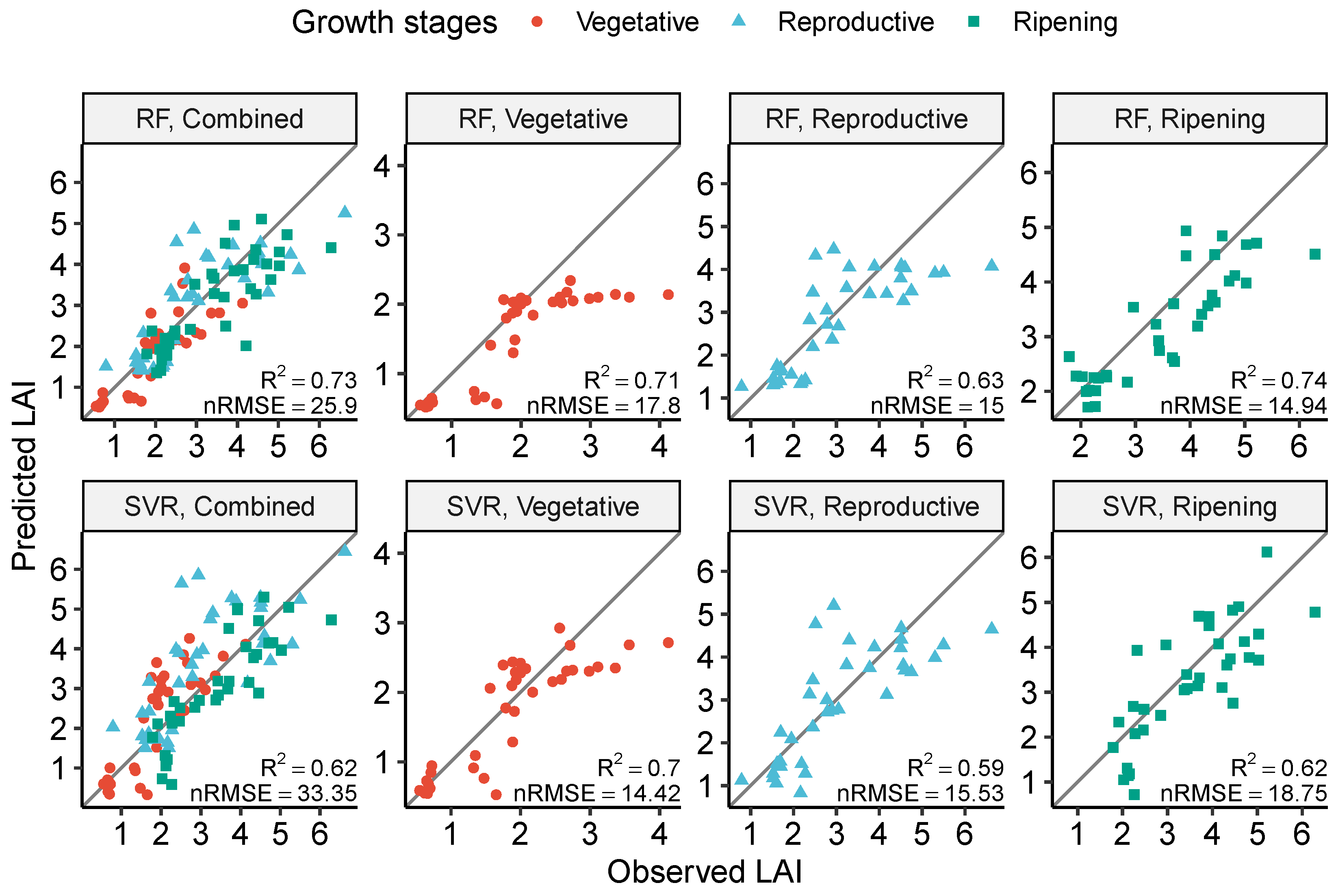
Therefore, the RF and SVR methods on first-derivative spectra are more suitable for building LAI estimation models. Table 6 shows the validation results of the RF and SVR models on first-derivative spectra (RF-D1, SVR-D1). Among them, the RF-D1 and SVR-D1 models of the whole growing season (RF-D1-EN, SVR-D1-EN) were validated on each separate growth stage data of the 2017 growing season, while the RF-D1 and SVR-D1 models of each single growth stage were validated on the corresponding growth stage data of the 2017 growing season. Figure 7 shows the relationships between the observed and predicted LAI along the 1:1 line on the standalone validation dataset of these models.
The RF-D1-VE (single growth stage RF-D1 model of vegetative growth stage) yielded validation and of 17.80% and 0.71. The RF-D1-RP and RF-D1-RI (single growth stage RF-D1 models of reproductive and ripening growth stages, respectively) models yielded validation of 15.00% and 14.90%, as well as validation of 0.63 and 0.74, respectively. When validated on each separate single growth data of the year 2017, the RF-D1-EN model yielded and of 14.90% and 0.71 for the vegetative growth stage, 14.10% and 0.64 for the reproductive growth stage, as well as 17.20% and 0.67 for the ripening growth stage, respectively. When compared to the single growth stage specific validation of the RF-D1-EN model, the of the single growth stage models (RF-D1-VE, RF-D1-RP and RF-D1-RI ) showed decrease ratios of −19.52%, −6.43% and 13.29% for the vegetative, reproductive and ripening growth stages, respectively. The increase ratios of the validation were −1.13%, −2.88% and 10.78% for the vegetative, reproductive and ripening growth stages, respectively. This result indicates that building RF-method-based LAI estimation models over a single growth stage rather than the whole growing season would increase the estimation accuracy for the ripening growth stage but decrease the estimation accuracy for the vegetative and red-edge growth stages.
The SVR-D1-VE, SVR-D1-RP and SVR-D1-RI models yielded validation of 14.40%, 15.50% and 18.80%, respectively, as well as validation of 0.70, 0.59 and 0.62, respectively. When validated on each separate single growth data of 2017 growing season, the SVR-D1-EN model yielded and of 22.10% and 0.70 for the vegetative growth stage, 19.70% and 0.55 for the reproductive growth stage, as well as 17.80% and 0.71 for the ripening growth stage, respectively. When compared to the single growth stage specific validation of the SVR-RF-EN model, the of the single growth stage models (SVR-D1-VE, SVR-D1-RP and SVR-D1-RI) showed decrease ratios of 34.66%, 21.18% and −5.58% for the vegetative, reproductive and ripening growth stages, respectively. The increase ratios of the validation were 1.03%, 8.09% and −12.47% for the vegetative, reproductive and ripening growth stages, respectively. This result indicates that building an SVR based LAI estimation model over a single growth stage rather than over the whole growing season would increase the estimation accuracy for the vegetative and reproductive growth stages but decrease the estimation accuracy for the ripening growth stage.
Considering the validation accuracy of the top performance VI models, RF and SVR models (Table 5 and Table 6) together, the provided the best paddy rice LAI estimation accuracy for the vegetative growth stage, and the RF-D1-RI model provided the best paddy rice LAI estimation accuracy for the ripening growth stage. No whole growing season models or other single growth stage models could provide better accuracy for these two growth stages. For the reproductive growth stage, the single growth VI model of , the RF-D1-RP model and the RF-D1-EN model all provided comparable accuracy. Thus, single growth stage models are recommended to build LAI estimation models. The VI model of and RF-D1-RI model are best options for vegetative and ripening growth stages, respectively. Considering the low computational cost of the VI method, the VI model of is the best option for reproductive growth stage.
4. Discussion
The optimal band pairs to formulate narrowband DVI, NDVI and SR were determined within each single growth stage and for the whole growing season of paddy rice in this study. The result showed that the optimal band pairs were almost identical within each growth stage or the whole growing season for these three indices. These band pairs generally have one band in the red-edge region around 750 nm and the other band in the NIR region, which was around 830 nm for the whole growing season and vegetative growth stage, around 1130 nm for the reproductive growth stage and around 860 nm for the ripening growth stage. These three indices with optimized band pairs showed clearly superior performance to the remaining seven VIs evaluated in this study. Because of the multiple scattering of light in canopies, the reflectance of NIR bands increases as LAI increases [50]. Furthermore, the importance of red-edge bands for LAI estimation have been demonstrated in previous studies [22,24,25,51]. These factors may be the reason why simple VIs based on the red-edge and NIR bands have strong correlations with LAI. Previous studies [22,23,24,51] showed that the common broadband red channel center onboard the current generation of earth-orbiting satellites is not the best choice to calculate the NDVI and also highlighted the importance of red-edge bands. Our results are consistent with these studies in that all optimal band pairs contain one red-edge band.
The best performance VI model for ripening growth stage provided lower accuracy than the top performance VI models of other growth stage with validation and at 20.21% and 0.39 respectively. A possible reason is that, at this growth stage, the existence of paddy rice panicle adds additional disturbance to the canopy spectra. Besides, the VIs that only use two spectra bands may be too simple for capturing the relationship between the canopy spectra and LAI. Furthermore, the VIs are designed to enhance green vegetation single [23], thus are more correlated with the green LAI. The SunScan Canopy Analysis System was used to determine field LAI in this study. The SunScan instrument is known influenced by non-photosynthetic components, and this problem is more obvious at the reproductive and ripening growth stages. This may additional reduce the goodness-of-fit of the ripening growth stage VI models. A previous study [52] showed that the LAI value determined by SunScan instrument is highly correlated with the destructive sample LAI when LAI < 4 for paddy rice. However, when LAI > 4, compared to the destructive method, this instrument may underestimate the LAI value. Whether this problem caused the relatively higher estimation error for reproductive and ripening growth stages will be considered in our future study.
Among the four multivariate calibration techniques evaluated in this study, the RF and SVR methods showed clearly better performance than the ANN and PLSR methods. The suboptimal performance of the ANN model may be due to the insufficient model calibration samples such that the solution may fall into a low local minima. The PLSR models yielded almost comparable accuracy with the corresponding RF and SVR models but provided a less accurate validation results. These results suggested that the PLSR models are less robust than the machine learning methods. The excellent performance of the RF model may be explained by its ’majority vote’ principle that has high tolerance to outliers.
In this study, the top-performing VI model for the whole growing season provided validation and of 36.86% and 0.58 (Figure 5), respectively, while the RF-D1-EN model provided validation and of 25.9% and 0.73, respectively. These results are consistent with previous studies in that the machine learning methods appear to be more efficient than the VI methods. However, when comparisons were made within specific single growth stages, this advantage was found only at the ripening growth stage. At the vegetative growth stage, the single growth stage VI model yielded lower and higher than both the single growth stage RF and SVR models. At the reproductive growth stage, the single growth stage VI model yielded comparable accuracy with the single growth stage RF model and lower and higher than the single growth stage SVR model. These results suggested that the machine learning methods only show an advantage in the late growing season when the canopy has a high LAI value, while in the early and middle growing season when the canopy has a lower LAI value, the VI method is still a reasonable option.
5. Conclusions
The univariate regression method on vegetation indices (VIs), traditional multivariate calibration method partial least squares regression (PLSR) and modern machine learning methods such as support vector regression (SVR), random forests (RF), and artificial neural networks (ANN) based on the original and first-derivative hyperspectral data were evaluated in this study for paddy rice LAI estimation with a special focus on the effects of growth stage development. All models were built on the whole growing season and on each separate vegetative, reproductive and ripening growth stage of paddy rice. The performance comparisons were made on each separate growth stage. Moreover, the optimal band pairs to calculate narrowband DVI, NDVI and SR were determined separately for each separate growth stage and the whole growing season.
The results showed that the optimal band pairs for narrowband DVI, NDVI and SR were generally the same within each growth stage. There was one band in the red-edge region around 750 nm, and the other band was in the NIR region, which was around 830 nm for the whole growing season and vegetative growth stage, around 1130 nm for the reproductive growth stage and around 860 nm for the ripening growth stage. The narrowband DVI, NDVI and SR showed clearly better performance than the other commonly used VIs. Specifically, , , and have the best performance for the whole growing season, vegetative, reproductive and ripening growth stages, respectively. Among the PLSR and three machine learning methods, the RF and SVR models yielded more accurate results than the corresponding PLSR and ANN models. For the RF and SVR methods, the models built on the first-derivative spectra showed advantage over the the corresponding models built on the original spectra.
Taking both the whole growing season and single growth stage VI, SVR and RF models into account together, the single growth stage VI model of provided the best paddy rice LAI estimation accuracy for the vegetative growth stage. The single growth stage RF model on D1 spectra provided the best paddy rice LAI estimation accuracy for the ripening growth stage. For the reproductive growth stage, the single growth VI model of , the single growth stage RF model on first-derivative spectra and the whole growing season RF model on first-derivative spectra all provided comparable accuracy. Furthermore, the whole growing season RF model on first-derivative spectra could proved reasonable accuracy for each single growth stage.
Author Contributions
Q.C., F.L. and L.W. conceived and designed the experiment. L.W., L.Y., Y.H., Q.W. and L.L. conducted the experiment. L.W. conducted the data analysis and prepared the manuscript. Q.C. and F.L. revised the manuscript. All authors read and approved the final version.
Funding
This work is supported by the Natural Sciences Foundation of China (41701398), the Hi-Tech Research and Development Program (863) of China (2013AA102401-2) and the Chinese Universities Scientific Fund (2452017108).
Acknowledgments
We acknowledge the kind help given by the Institute of Agricultural Resources and Environment, Ningxia Academy of Agro-forestry Science, Yinchuan.
Conflicts of Interest
The authors declare no conflict of interest.
References
- Zheng, G.; Moskal, L.M. Retrieving Leaf Area Index (LAI) Using Remote Sensing: Theories, Methods and Sensors. Sensors 2009, 9, 2719–2745. [Google Scholar] [CrossRef] [PubMed] [Green Version]
- Atzberger, C. Advances in remote sensing of agriculture: Context description, existing operational monitoring systems and major information needs. Remote Sens. 2013, 5, 949–981. [Google Scholar] [CrossRef]
- Feng, R.; Zhang, Y.; Yu, W.; Hu, W.; Wu, J.; Ji, R.; Wang, H.; Zhao, X. Analysis of the relationship between the spectral characteristics of maize canopy and leaf area index under drought stress. Acta Ecol. Sin. 2013, 33, 301–307. [Google Scholar] [CrossRef]
- Thorp, K.R.; Gore, M.A.; Andrade-Sanchez, P.; Carmo-Silva, A.E.; Welch, S.M.; White, J.W.; French, A.N. Proximal hyperspectral sensing and data analysis approaches for field-based plant phenomics. Comput. Electron. Agric. 2015, 118, 225–236. [Google Scholar] [CrossRef] [Green Version]
- Vaesen, K.; Gilliams, S.; Nackaerts, K.; Coppin, P. Ground-measured spectral signatures as indicators of ground cover and leaf area index: the case of paddy rice. Field Crops Res. 2001, 69, 13–25. [Google Scholar] [CrossRef]
- Jin, X.; Kumar, L.; Li, Z.; Feng, H.; Xu, X.; Yang, G.; Wang, J. A review of data assimilation of remote sensing and crop models. Eur. J. Agron. 2018, 92, 141–152. [Google Scholar] [CrossRef]
- Mokhtari, A.; Noory, H.; Vazifedoust, M. Improving crop yield estimation by assimilating LAI and inputting satellite-based surface incoming solar radiation into SWAP model. Agric. For. Meteorol. 2018, 250–251, 159–170. [Google Scholar] [CrossRef]
- Liu, K.; Zhou, Q.B.; Wu, W.B.; Xia, T.; Tang, H.J. Estimating the crop leaf area index using hyperspectral remote sensing. J. Integr. Agric. 2016, 15, 475–491. [Google Scholar] [CrossRef] [Green Version]
- Lee, K.S.; Cohen, W.B.; Kennedy, R.E.; Maiersperger, T.K.; Gower, S.T. Hyperspectral versus multispectral data for estimating leaf area index in four different biomes. Remote Sens. Environ. 2004, 91, 508–520. [Google Scholar] [CrossRef]
- Schlerf, M.; Atzberger, C.; Hill, J. Remote sensing of forest biophysical variables using HyMap imaging spectrometer data. Remote Sens. Environ. 2005, 95, 177–194. [Google Scholar] [CrossRef] [Green Version]
- Pu, R.; Gong, P.; Yu, Q. Comparative Analysis of EO-1 ALI and Hyperion, and Landsat ETM+ Data for Mapping Forest Crown Closure and Leaf Area Index. Sensors 2008, 8, 3744–3766. [Google Scholar] [CrossRef] [PubMed] [Green Version]
- Verrelst, J.; Alonso, L.; Camps-Valls, G.; Delegido, J.; Moreno, J. Retrieval of Vegetation Biophysical Parameters Using Gaussian Process Techniques. IEEE Trans. Geosci. Remote Sens. 2012, 50, 1832–1843. [Google Scholar] [CrossRef]
- Duan, S.B.; Li, Z.L.; Wu, H.; Tang, B.H.; Ma, L.; Zhao, E.; Li, C. Inversion of the PROSAIL model to estimate leaf area index of maize, potato, and sunflower fields from unmanned aerial vehicle hyperspectral data. Int. J. App. Earth Obs. Geoinform. 2014, 26, 12–20. [Google Scholar] [CrossRef]
- Kiala, Z.; Odindi, J.; Mutanga, O.; Peerbhay, K. Comparison of partial least squares and support vector regressions for predicting leaf area index on a tropical grassland using hyperspectral data. J. Appl. Remote Sens. 2016, 10, 036015. [Google Scholar] [CrossRef]
- Yuan, H.; Yang, G.; Li, C.; Wang, Y.; Liu, J.; Yu, H.; Feng, H.; Xu, B.; Zhao, X.; Yang, X.; et al. Retrieving Soybean Leaf Area Index from Unmanned Aerial Vehicle Hyperspectral Remote Sensing: Analysis of RF, ANN, and SVM Regression Models. Remote Sens. 2017, 9, 309. [Google Scholar] [CrossRef]
- Wu, C.; Han, X.; Niu, Z.; Dong, J. An evaluation of EO-1 hyperspectral Hyperion data for chlorophyll content and leaf area index estimation. Int. J. Remote Sens. 2010, 31, 1079–1086. [Google Scholar] [CrossRef]
- Berger, K.; Atzberger, C.; Danner, M.; D’Urso, G.; Mauser, W.; Vuolo, F.; Hank, T. Evaluation of the PROSAIL Model Capabilities for Future Hyperspectral Model Environments: A Review Study. Remote Sens. 2018, 10, 85. [Google Scholar] [CrossRef]
- Verrelst, J.; Malenovský, Z.; Van der Tol, C.; Camps-Valls, G.; Gastellu-Etchegorry, J.P.; Lewis, P.; North, P.; Moreno, J. Quantifying Vegetation Biophysical Variables from Imaging Spectroscopy Data: A Review on Retrieval Methods. Surv. Geophys. 2018. [Google Scholar] [CrossRef]
- Rouse, J.W.; Haas, R.H.; Schell, J.A.; Deering, D.W. Monitoring Vegetation Systems in the Great Okains with ERTS. In Proceedings of the Third Earth Resources Technology Satellite-1 Symposium, Washington, DC, USA, 10–14 December 1973; Volume 1, pp. 325–333. [Google Scholar]
- Jordan, C.F. Derivation of Leaf-Area Index from Quality of Light on the Forest Floor. Ecology 1969, 50, 663–666. [Google Scholar] [CrossRef]
- Richardson, A.J.; Wiegand, C.L. Distinguishing vegetation from soil background information. Photogramm. Eng. Remote Sens. 1977, 43, 1541–1552. [Google Scholar]
- Hansen, P.M.; Schjoerring, J.K. Reflectance measurement of canopy biomass and nitrogen status in wheat crops using normalized difference vegetation indices and partial least squares regression. Remote Sens. Environ. 2003, 86, 542–553. [Google Scholar] [CrossRef]
- Zhao, D.; Huang, L.; Li, J.; Qi, J. A comparative analysis of broadband and narrowband derived vegetation indices in predicting LAI and CCD of a cotton canopy. ISPRS J. Photogramm. Remote Sens. 2007, 62, 25–33. [Google Scholar] [CrossRef]
- Delegido, J.; Verrelst, J.; Meza, C.M.; Rivera, J.P.; Alonso, L.; Moreno, J. A red-edge spectral index for remote sensing estimation of green LAI over agroecosystems. Eur. J. Agron. 2013, 46, 42–52. [Google Scholar] [CrossRef]
- Tanaka, S.; Kawamura, K.; Maki, M.; Muramoto, Y.; Yoshida, K.; Akiyama, T. Spectral Index for Quantifying Leaf Area Index of Winter Wheat by Field Hyperspectral Measurements: A Case Study in Gifu Prefecture, Central Japan. Remote Sens. 2015, 7, 5329–5346. [Google Scholar] [CrossRef] [Green Version]
- Camps-Valls, G.; Bruzzone, L.; Rojo-Rojo, J.L.; Melgani, F. Robust Support Vector Regression for Biophysical Variable Estimation From Remotely Sensed Images. IEEE Geosci. Remote Sens. Lett. 2006, 3, 339–343. [Google Scholar] [CrossRef]
- Cho, M.A.; Skidmore, A.; Corsi, F.; van Wieren, S.E.; Sobhan, I. Estimation of green grass/herb biomass from airborne hyperspectral imagery using spectral indices and partial least squares regression. Int. J. Appl. Earth Obs. Geoinformation 2007, 9, 414–424. [Google Scholar] [CrossRef]
- Darvishzadeh, R.; Skidmore, A.; Schlerf, M.; Atzberger, C.; Corsi, F.; Cho, M. LAI and chlorophyll estimation for a heterogeneous grassland using hyperspectral measurements. ISPRS J. Photogramm. Remote Sens. 2008, 63, 409–426. [Google Scholar] [CrossRef]
- Wang, L.; Chang, Q.; Yang, J.; Zhang, X.; Li, F. Estimation of paddy rice leaf area index using machine learning methods based on hyperspectral data from multi-year experiments. PLoS ONE 2018, 13, e0207624. [Google Scholar] [CrossRef] [PubMed]
- Wang, F.M.; Huang, J.F.; Lou, Z.H. A comparison of three methods for estimating leaf area index of paddy rice from optimal hyperspectral bands. Precis. Agric. 2011, 12, 439–447. [Google Scholar] [CrossRef]
- Liu, R.L.; Zhang, A.P.; Li, Y.H.; Wang, F.; Zhao, T.C.; Chen, C.; Hong, Y. Rice Yield, Nitrogen Use Efficiency (NUE) and Nitrogen Leaching Losses as Affected by Long-term Combined Applications of Manure and Chemical Fertilizers in Yellow River Irrigated Region of Ningxia, China. J. Agro-Environ. Sci. 2015, 34, 947–954. [Google Scholar] [CrossRef]
- Tsai, F.; Philpot, W. Derivative Analysis of Hyperspectral Data. Remote Sens. Environ. 1998, 66, 41–51. [Google Scholar] [CrossRef]
- Moldenhauer, K.; Slaton, N. Rice Growth and Development. In Rice Production Handbook; University of Arkansas: Fayetteville, AR, USA, 2001; pp. 7–14. [Google Scholar]
- R Core Team. R: A Language and Environment for Statistical Computing; R Core Team: Vienna, Austria, 2018. [Google Scholar]
- Mevik, B.H.; Wehrens, R. The pls Package: Principal Component and Partial Least Squares Regression in R. J. Stat. Softw. 2014, 59, 1–23. [Google Scholar]
- Liaw, A.; Wiener, M. Classification and Regression by randomForest. R News 2002, 2, 18–22. [Google Scholar]
- Karatzoglou, A.; Smola, A.; Hornik, K.; Zeileis, A. kernlab—An S4 Package for Kernel Methods in R. J. Stat. Softw. 2004, 11, 1–20. [Google Scholar] [CrossRef]
- Chollet, F.; Allaire, J.J. R Interface to Keras. 2017. Available online: https://github.com/rstudio/keras (accessed on 12 October 2018).
- Abadi, M.; Barham, P.; Chen, J.; Chen, Z.; Davis, A.; Dean, J.; Devin, M.; Ghemawat, S.; Irving, G.; Isard, M.; et al. TensorFlow: A system for large-scale machine learning. In Proceedings of the 12th USENIX Symposium on Operating Systems Design and Implementation (OSDI 16), Savannah, GA, USA, 2–4 November 2016; pp. 265–283. [Google Scholar]
- Qi, J.; Chehbouni, A.; Huete, A.R.; Kerr, Y.H.; Sorooshian, S. A modified soil adjusted vegetation index. Remote Sens. Environ. 1994, 48, 119–126. [Google Scholar] [CrossRef]
- Huete, A.R.; Liu, H.Q.; Batchily, K.; Van Leeuwen, W. A comparison of vegetation indices over a global set of TM images for EOS-MODIS. Remote Sens. Environ. 1997, 59, 440–451. [Google Scholar] [CrossRef]
- Gitelson, A.A. Wide Dynamic Range Vegetation Index for remote quantification of biophysical characteristics of vegetation. J. Plant Physiol. 2004, 161, 165–173. [Google Scholar] [CrossRef]
- Dash, J.; Curran, P.J. The MERIS terrestrial chlorophyll index. Int. J. Remote Sens. 2004, 25, 5403–5413. [Google Scholar] [CrossRef]
- Broge, N.H.; Leblanc, E. Comparing prediction power and stability of broadband and hyperspectral vegetation indices for estimation of green leaf area index and canopy chlorophyll density. Remote Sens. Environ. 2001, 76, 156–172. [Google Scholar] [CrossRef]
- Wold, S.; Sjöström, M.; Eriksson, L. PLS-regression: A basic tool of chemometrics. Chemom. Intell. Lab. Syst. 2001, 58, 109–130. [Google Scholar] [CrossRef]
- Smola, A.J.; Schölkopf, B. A Tutorial on Support Vector Regression. Stat. Comput. 2004, 14, 199–222. [Google Scholar] [CrossRef]
- Breiman, L. Random Forests. Mach. Learn. 2001, 45, 5–32. [Google Scholar] [CrossRef] [Green Version]
- Atkinson, P.M.; Tatnall, A.R.L. Introduction neural networks in remote sensing. Int. J. Remote Sens. 1997, 18, 699–709. [Google Scholar] [CrossRef]
- Kingma, D.P.; Ba, J. Adam: A Method for Stochastic Optimization. Available online: https://arxiv.org/abs/1412.6980 (accessed on 11 February 2019).
- Filella, I.; Penuelas, J. The red edge position and shape as indicators of plant chlorophyll content, biomass and hydric status. Int. J. Remote Sens. 1994, 15, 1459–1470. [Google Scholar] [CrossRef]
- Delegido, J.; Verrelst, J.; Alonso, L.; Moreno, J. Evaluation of Sentinel-2 Red-Edge Bands for Empirical Estimation of Green LAI and Chlorophyll Content. Sensors 2011, 11, 7063–7081. [Google Scholar] [CrossRef] [PubMed] [Green Version]
- Sone, C.; Saito, K.; Futakuchi, K. Comparison of three methods for estimating leaf area index of upland rice cultivars. Crop Sci. 2009, 49, 1438–1443. [Google Scholar] [CrossRef]
Figure 1.
Demonstration of biochar and nitrogen treatments. The field was treated with three nitrogen rates (N0, N1 and N2) and four biochar rates (C0, C1, C2 and C3).
Figure 1.
Demonstration of biochar and nitrogen treatments. The field was treated with three nitrogen rates (N0, N1 and N2) and four biochar rates (C0, C1, C2 and C3).

Figure 2.
Boxplot of measured leaf area index (LAI).

Figure 3.
Calibration counterplot for linear regression models built on difference vegetative index (DVI), normalized difference vegetation index (NDVI) and simple ratio vegetation index (SR) (Table 2) with all possible two band pair combinations against LAI.
Figure 3.
Calibration counterplot for linear regression models built on difference vegetative index (DVI), normalized difference vegetation index (NDVI) and simple ratio vegetation index (SR) (Table 2) with all possible two band pair combinations against LAI.

Figure 4.
Calibration (with cross-validation procedure (CV)) and validation of different vegetation indexes (VIs) for the whole growing season and each single growth stage.
Figure 4.
Calibration (with cross-validation procedure (CV)) and validation of different vegetation indexes (VIs) for the whole growing season and each single growth stage.

Figure 5.
Observed vs. predicted LAI along the 1:1 line on standalone validation dataset of the best-performing VI models (in Table 5).
Figure 5.
Observed vs. predicted LAI along the 1:1 line on standalone validation dataset of the best-performing VI models (in Table 5).

Figure 6.
Calibration (with CV) and validation of different multivariate calibration methods. The whole growing season and single growth stage models built on original and first-derivative spectra are shown in different panels.
Figure 6.
Calibration (with CV) and validation of different multivariate calibration methods. The whole growing season and single growth stage models built on original and first-derivative spectra are shown in different panels.

Figure 7.
Observed vs. predicted LAI along the 1:1 line on standalone validation dataset of the random forests (RF) and support vector regression (SVR) models on first-derivative spectra. ‘Combined’ means the whole growing season model. ‘Vegetative’, ‘Reproductive’ and ‘Ripening’ mean the single growth stage model of the specific growth stages.


Table 1.
Day after transplantation (DAT) on which the data collection campaigns were conducted.
| Growth Stages | 2014 | 2015 | 2016 | 2017 |
|---|---|---|---|---|
| Vegetative | 44 | 41 | 48 | 46 |
| Reproductive | 75 | 70 | 81 | 78 |
| Ripening | 94 | 90 | 103 | 110 |
Table 2.
Vegetation indices evaluated in this study.
| Index | Formula | Cite |
|---|---|---|
| DVI | [21] | |
| NDVI | [19] | |
| SR | [20] | |
| EVI | [41] | |
| WDRVI | [42] | |
| MSAVI | [40] | |
| [16] | ||
| MTCI | [43] | |
| lp | red edge position | [23] |
| Rp | reflectance at lp | [23] |
stands for reflectance at band nm.; was used.
Table 3.
Descriptive statistics of measured leaf area index (LAI) for each single growth stage and for the whole growing season.
Table 3.
Descriptive statistics of measured leaf area index (LAI) for each single growth stage and for the whole growing season.
| Dataset | Sample Number | Min | Max | Mean | SD |
|---|---|---|---|---|---|
| Whole dataset | 419 | 0.08 | 7.35 | 2.55 | 1.63 |
| Vegetative | 135 | 0.08 | 4.12 | 1.37 | 0.96 |
| Reproductive | 142 | 0.65 | 6.62 | 2.88 | 1.45 |
| Ripening | 142 | 0.72 | 7.35 | 3.33 | 1.69 |
Table 4.
Band combinations that yielded the highest to predict paddy rice leaf area index (LAI) of the difference vegetative index (DVI), normalized difference vegetation index (NDVI) and simple ratio vegetation index (SR) for whole growing season and each single growth stage.
Table 4.
Band combinations that yielded the highest to predict paddy rice leaf area index (LAI) of the difference vegetative index (DVI), normalized difference vegetation index (NDVI) and simple ratio vegetation index (SR) for whole growing season and each single growth stage.
| Dataset | ||||||
|---|---|---|---|---|---|---|
| Bands (nm) | Bands (nm) | Bands (nm) | ||||
| Whole growing season | (766, 826) | 0.71 | (762, 828) | 0.65 | (762, 828) | 0.65 |
| Vegetative | (744, 944) | 0.82 | (752, 826) | 0.84 | (750, 826) | 0.84 |
| Reproductive | (736, 1124) | 0.71 | (740, 1128) | 0.64 | (744, 1128) | 0.64 |
| Ripening | (754, 860) | 0.70 | (750, 860) | 0.61 | (752, 858) | 0.61 |
Table 5.
The validation and of top-performing vegetation index (VI) models for whole growing season and each separate growth stage. The whole growing season model was validated on each separate growth stage data of the 2017 growing season.
Table 5.
The validation and of top-performing vegetation index (VI) models for whole growing season and each separate growth stage. The whole growing season model was validated on each separate growth stage data of the 2017 growing season.
| Validation Dataset | Whole Growing Season Model | Single Growth Stage Models | Differences | |||
|---|---|---|---|---|---|---|
| vegetative | 18.90 | 0.67 | 14.00 | 0.79 | 25.60 | 16.71 |
| reproductive | 17.10 | 0.59 | 15.20 | 0.63 | 10.80 | 6.73 |
| ripening | 29.20 | 0.24 | 20.20 | 0.39 | 30.70 | 61.54 |
model for the whole growing season. They are models of , and for vegetative, reproductive and ripening growth stages, respectively. , .
Table 6.
The validation and of random forests (RF) and support vector regression (SVR) models on first-derivative spectra for the whole growing season and each single growth stage. The whole growing season models were validated on each separate growth stage data of the 2017 growing season.
Table 6.
The validation and of random forests (RF) and support vector regression (SVR) models on first-derivative spectra for the whole growing season and each single growth stage. The whole growing season models were validated on each separate growth stage data of the 2017 growing season.
| Method | Validation Dataset | Whole Growing Season Model | Single Growth Stage Model | Difference | |||
|---|---|---|---|---|---|---|---|
| RF | Vegetative | 14.90 | 0.71 | 17.80 | 0.71 | −19.52 | −1.13 |
| Reproductive | 14.10 | 0.64 | 15.00 | 0.63 | −6.43 | −2.88 | |
| Ripening | 17.20 | 0.67 | 14.90 | 0.74 | 13.29 | 10.78 | |
| SVR | Vegetative | 22.10 | 0.70 | 14.40 | 0.70 | 34.66 | 1.03 |
| Reproductive | 19.70 | 0.55 | 15.50 | 0.59 | 21.18 | 8.09 | |
| Ripening | 17.80 | 0.71 | 18.80 | 0.62 | −5.58 | −12.47 | |
, .
© 2019 by the authors. Licensee MDPI, Basel, Switzerland. This article is an open access article distributed under the terms and conditions of the Creative Commons Attribution (CC BY) license (http://creativecommons.org/licenses/by/4.0/).
Share and Cite
MDPI and ACS Style
Wang, L.; Chang, Q.; Li, F.; Yan, L.; Huang, Y.; Wang, Q.; Luo, L. Effects of Growth Stage Development on Paddy Rice Leaf Area Index Prediction Models. Remote Sens. 2019, 11, 361. https://0-doi-org.brum.beds.ac.uk/10.3390/rs11030361
AMA Style
Wang L, Chang Q, Li F, Yan L, Huang Y, Wang Q, Luo L. Effects of Growth Stage Development on Paddy Rice Leaf Area Index Prediction Models. Remote Sensing. 2019; 11(3):361. https://0-doi-org.brum.beds.ac.uk/10.3390/rs11030361
Chicago/Turabian StyleWang, Li, Qingrui Chang, Fenling Li, Lin Yan, Yong Huang, Qi Wang, and Lili Luo. 2019. "Effects of Growth Stage Development on Paddy Rice Leaf Area Index Prediction Models" Remote Sensing 11, no. 3: 361. https://0-doi-org.brum.beds.ac.uk/10.3390/rs11030361
Note that from the first issue of 2016, this journal uses article numbers instead of page numbers. See further details here.