Addressing Challenges for Mapping Irrigated Fields in Subhumid Temperate Regions by Integrating Remote Sensing and Hydroclimatic Data

Abstract

High-resolution mapping of irrigated fields is needed to better estimate water and nutrient fluxes in the landscape, food production, and local to regional climate. However, this remains a challenge in humid to subhumid regions, where irrigation has been expanding into what was largely rainfed agriculture due to trends in climate, crop prices, technologies and practices. One such region is southwestern Michigan, USA, where groundwater is the main source of irrigation water for row crops (primarily corn and soybeans). Remote sensing of irrigated areas can be difficult in these regions as rainfed areas have similar characteristics. We present methods to address this challenge and enhance the contrast between neighboring rainfed and irrigated areas, including weather-sensitive scene selection, applying recently developed composite indices and calculating spatial anomalies. We create annual, 30m-resolution maps of irrigated corn and soybeans for southwestern Michigan from 2001 to 2016 using a machine learning method (random forest). The irrigation maps reasonably capture the spatial and temporal pattern of irrigation, with accuracies that exceed available products. Analysis of the irrigation maps showed that the irrigated area in southwestern Michigan tripled in the last 16 years. We also discuss the remaining challenges for irrigation mapping in humid to subhumid areas.

1. Introduction

Agriculture is the sector with the largest consumptive use of water across the globe. While crop water demand is largely met by irrigation in arid to semiarid regions, farmers in humid regions traditionally rely on rainfall. However, irrigation has become more common in humid to subhumid regions [1], driven by the growth of demand for corn grain bioethanol, the need to increase yield given current low prices of corns and soybeans [2], the ready availability of more water and energy efficient irrigation technologies, and increasing climate variability.

The rapid expansion of irrigation has important implications for terrestrial water balances, food production, and local to regional climate [3,4,5,6]. Land surface models have been increasingly used as quantitative tools to estimate the effects of land use change and other human activities on terrestrial water and energy cycles. However, these models require high-resolution observations at the model scale to fully vet the irrigated area [7,8]. Thus, detailed depiction of spatiotemporal patterns of irrigation is needed for modelers and decision makers [9]. However, accurate monitoring of irrigated area can be difficult in humid to subhumid regions (hereafter humid regions), primarily because of the similarity of signals from rainfed and irrigated areas in such regions [10].

Remote sensing provides valuable information to delineate irrigated areas. Within the U.S., the Moderate Resolution Imaging Spectroradiometer (MODIS) Irrigated Agriculture Dataset for the United States (MIrAD-US) national irrigation dataset was developed by the U.S. Geological Survey (USGS) by integrating U.S. Department of Agriculture (USDA) county statistics, MODIS satellite imagery and a national land cover map [11]. The MIrAD-US product has 250-m resolution and is available in 2002, 2007 and 2012. MIrAD-US revealed significant temporal variability and suggests the need for regular periodic mapping of irrigated areas [12]. Later studies have used higher resolution imagery (10–30 m) from Landsat and Sentinel-1 satellites to develop more detailed irrigation maps for local to regional studies [13,14,15]. In particular, annual irrigation maps were developed for the Republican River Basin from 1999 to 2016 (AIM-RRB), leveraging recent advances in cloud computing, machine learning, and increasingly accessible Landsat data [13].

In southwestern Michigan, a subhumid region in the midwestern U.S., water consumption by agriculture has rapidly increased over the past two decades. Irrigation of row crops (primarily corn and soybean) was once practiced only on a small fraction of the total crop land across the upper Midwest. However, in the last two decades there has been a dramatic expansion in irrigation use [2], mostly from groundwater pumping [16]. Large acreages of fields in southwestern Michigan are devoted to producing seed corn, commercial corn, and soybeans [16]. The prevailing sandy soils [17] and shallow depths to groundwater [18] in this region allows adoption of central pivot irrigation systems with limited operation costs. Given the strong connection between groundwater and surface water, irrigation in southwestern Michigan has the potential to reduce the health of some local surface water ecosystems [19].

Remote sensing methods are able to map irrigated fields in arid and semi-arid environments with satisfactory accuracy, however the accuracy of satellite-based irrigation mapping techniques in more humid regions is still unknown [11]. The objective of this study was to create high-resolution, annual maps of irrigated fields in a sub-humid region by integrating remote sensing imagery with climate and land surface modeling data. We identified three methods to increase remote sensing accuracy: (1) use weather-sensitive selection of imagery timing, (2) test the transferability of recently-developed composite indices for detecting irrigation in arid areas [13] to humid regions, and (3) calculate spatial anomaly indices. We demonstrated this approach in southwestern Michigan (SW MI) where corn and soybeans are the two principal irrigated crops. We also evaluated the accuracy of irrigation mapping under various climate conditions in this region, which provided insights into the applicability to other humid regions.

2. Materials and Methods

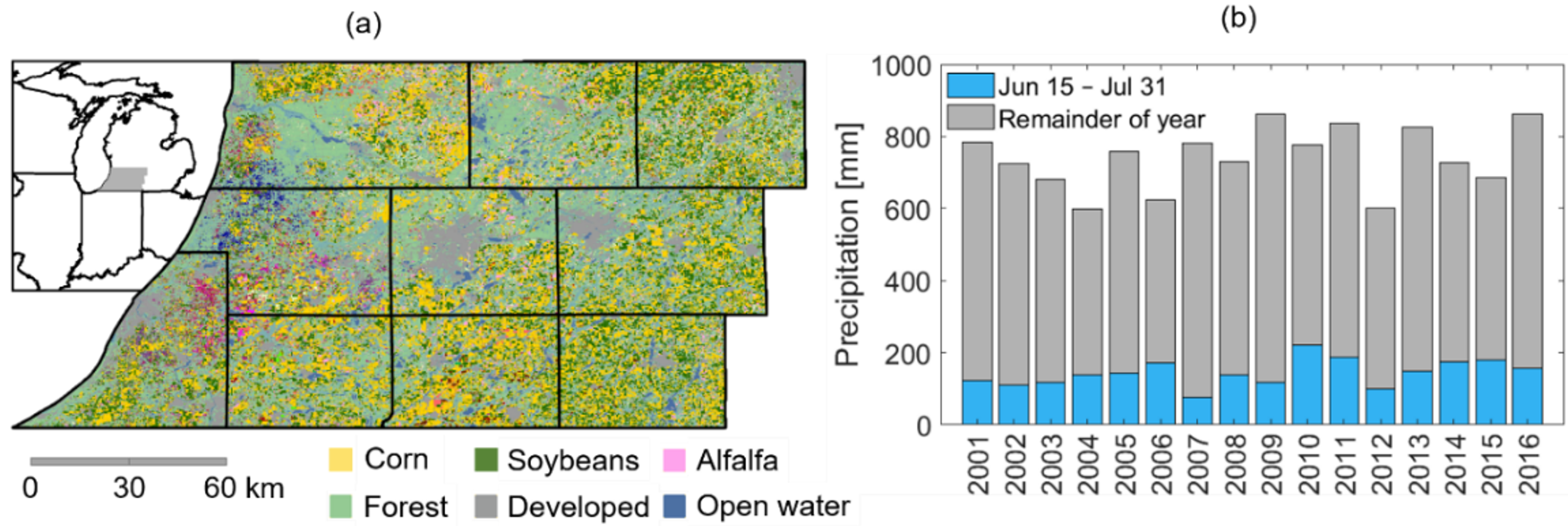
2.1. Study Area

In this study, we considered ten counties (Allegan, Barry, Eaton, van Buren, Kalamazoo, Calhoun, Berrien, Cass, St. Joseph and Branch) covering 28,281 km² in southwestern Michigan (Figure 1a). The study area is part of the US Corn Belt with a subhumid climate [20], with annual precipitation ranging from 590 mm (in the 2012 drought) to 858 mm during the study period 2001–2016 (Figure 1b, [21]). Short term droughts, common in this region, induce plant water stress and reduce grain yields of corn and soybeans, which account for 45% and 32% of total agricultural area, respectively [22]. During extended drought periods, the sandy soils prevalent in this region cannot store sufficient soil water to allow crops to reach full yield potential.

2.2. Basic Remotely Sensed, Land Surface Model, and Climate Input Data

We used a variety of time-varying and static input data for the random forest (RF) classification model (summarized in

Table 1. Basic input variables and indices used to calculate derived input variables.

Variable	Description	Source
EVI	Enhanced Vegetation Index	Landsat
GI	Green Index	Landsat
NDWI	Normalized Difference Water Index	Landsat
NDVI	Normalized Difference Vegetation Index	Landsat
Thermal	Landsat 5 & 7: 10.40–12.50 µm band Landsat 8: 11.50–12.51 µm band	Landsat
Dryspell	See text	Derived: PRISM
P	Precipitation	PRISM
VPD	Mean daily max. vapor pressure deficit	PRISM
GDD	Growing degree-day	PRISM
Aridity	Total precipitation/PET, May–Aug	Derived: GRIDMET
PDSI	Palmer Drought Severity Index	GRIDMET
Soil moisture	Root zone soil moisture	NLDAS-2 Noah
AWC	Available water capacity	SSURGO
Ksat	Vertical saturated hydraulic conductivity	SSURGO

and

Table 2. Weather-sensitive remote sensing, spatial anomaly and composite indices.

Group	Variable Code or Suffix	Description
Weather-sensitive remote sensing indices	VDPMaxGI	3-day average VPD before maximum Landsat GI day
	dryspellMaxGI	Number of consecutive days with rainfall ≤ 5 mm before maximum GI day
		NDVI, EVI, GI and NDWI calculated using the Landsat scene after a dry period identified using three criteria
	_SM	Descending soil moisture
	_pdsi	Lowest PDSI
	_ppt	Longest dryspell
Spatial anomaly indices		NDVI, EVI, GI and NDWI statistics subtracted by neighborhood %
	_p40	40%
	_p90	90%
Composite indices	WGI	Maximum GI $\times$ mean NDWI (water-adjusted GI, [13]
	AGI	Maximum GI/aridity (aridity normalized GI, [13]
	WGI_ppt, AGI_ppt	WGI and AGI calculated using GI from scenes that immediately follows a dry period

). The static input variables describe terrain, soil, and geographic location. Dynamic inputs are derived from remote sensing and climate data, as well as land surface model output. For most time varying data, we focus on the June 15th to July 31st period, which is the time before canopy closure occurs in corn and soybeans to avoid reflectance saturation. Data were either obtained from, or uploaded to, the Google Earth Engine (GEE) cloud computing platform [23] for classification.

We included five temporally static input variables to account for possible relations between yield and terrain attributes, soil properties, crop characteristics, and geographic information. These variables are: (1) slope calculated from 30-m National Elevation Dataset (NED) Digital Elevation Model (DEM) [24], (2) soil available water capacity (AWC, field capacity minus wilting point), (3) vertical saturated hydraulic conductivity (${\mathrm{k}}_{\mathrm{Sat}}$), (4) latitude (lat), and (5) longitude (long). The AWC and $k_{Sat}$ are based on the top 25 cm soil properties provided by the USDA Soil Survey Geographic Dataset (SSURGO) Web Soil Survey [17]. For each SSURGO map unit polygon, we calculated depth- and component-fraction weighted averages of all soil horizon textures (%sand, %clay) within the top 25 cm. We then used the ROSETTA database [25] to relate these textures to estimates of field capacity, wilting point, and soil hydraulic conductivity. Vertical hydraulic conductivity was calculated for each component as the harmonic mean of individual horizontal saturated conductivities.

Climate inputs were derived from daily 4-km resolution PRISM [21] and Gridded Surface Meteorological dataset (GRIDMET) [26]: (1) precipitation, (2) aridity calculated as the ratio of growing season rainfall to potential evapotranspiration (PET), (3) average Palmer Drought Severity Index (PDSI), (4) dryspell (maximum consecutive days with less than 5 mm precipitation), (5) average daily maximum VPD (vapor pressure deficit), (6) daily mean temperature, (7) heatwave (maximum consecutive days with daily mean temperature above 25 °C, (8) GDD (growing degree days = cumulative degree obtained from the difference between air temperature and base temperature for corn and soybeans, 25 °C in this study), and (9) as a measure of pre- and in season-wetness, we calculated the total precipitation before June 15th (p_early) and from June 15th to Jul. 31st (p_sum), respectively.

Irrigation decisions are often based on soil water content [8]. Here, we use the root zone soil water content at noon from NLDAS-Noah with 1/8° spatial resolution and hourly time step [27], which is currently the best readily available product at regional scale that has sufficiently fine temporal resolution for our application. The NLDAS-Noah product does not implement irrigation, thus its soil water content data serves as a reference that represents wetness under rainfed conditions.

We used remote sensing data from Landsat Surface Reflectance Products at an 8-day interval in all years except 2012, when there was a 16-day interval since only Landsat 7 ETM+ was operational. We included all scenes within 5 days of the June 15th to July 31st key growing season period. The actual number of available scenes during this period varies spatially and inter-annually as the 8-day (16-day in 2012) return interval is simultaneously reduced by cloud coverage and augmented by overlapping scene edges. From 2001 to 2016, the average number of valid observations among pixels in the study domain varied from 1.67 (2012) to 6.35 (2001) (Table S1, Supplementary Material). All Landsat 7 images collected after May 31, 2003 have data gaps due to the Scan Line Corrector (SLC) failure, which leads to significant data shortage in 2012. We used a moving window average method to fill in the gaps caused by the SLC failure. For every pixel within a gap, we set its value as the average within a five pixel by one pixel rectangle, oriented perpendicular to the scanline.

After filling the data gaps, we extracted the thermal, near-infrared, short-wave infrared, red, green, and blue bands from Landsat images between June 10th and August 5th and calculated NDVI, EVI, GI and NDWI. We then created statistical composites from the available imagery following a best pixel approach [28] to generate mean, maximum, minimum and range (i.e., maximum subtracted by minimum) composites for all four indices and the thermal band.

2.3. Weather-Sensitive Scene Selection, Spatial Anomaly Calculation, and Novel Composite Indices

Initially we applied the methods from previous studies (i.e., [12,13,14]) to construct a RF classifier for this region, but found the accuracies were inadequate. We thus developed and tested a variety of approaches, including several that we deemed unsuccessful because they did not increase the accuracy of the RF classifier. Ultimately, we implemented three methods to create layers beyond the basic remotely sensed, land surface model (LSM), and climate indices described in Section 2.2.

First, we calculated two composite indices recently proposed in [13] that adjust GI in an attempt to account for regional variations in available water. The first composite variable is the product of maximum GI and growing-season mean NDWI (i.e., water-adjusted green index, WGI); we anticipate that for irrigated fields GI and NDWI will both be high. A pixel with high GI but low NDWI may be rainfed (low NDWI) but treated with abundant nutrients (high GI). The other composite variable is maximum GI divided by seasonal aridity (i.e., aridity-normalized green index, AGI). The rationale behind AGI is that irrigated fields should have high GI even during relatively dry growing conditions.

Second, we developed weather-sensitive remote sensing indices calculated from Landsat scenes at the time most favorable for distinguishing irrigated from rainfed fields. We assumed this time immediately follows a dry period identified based on three separate criteria: (1) maximum consecutive days with monotonically descending root zone (up to 1-m depth) soil water content, (2) lowest PDSI of the season, and (3) greatest number of consecutive days with daily precipitation less than 5 mm. The criteria were calculated using climate and LSM model outputs listed in Table 1. The resulting input variables are denoted with suffix _SM, _pdsi, _ppt, respectively. Irrigated crops generally exhibit higher vegetation indices and NDWI than rainfed crops [13,14,27,29,30]; we expect that this difference is amplified under water stress conditions during dry periods. Further, the three-day average vapor pressure deficit (VPD) before the day of maximum Landsat GI (VPDMaxGI) and number of consecutive days with rainfall not exceeding 5 mm before maximum GI day (dryspellMaxGI), were calculated as rainfed crops are unlikely to exhibit maximum GI when VPD is high or after a dry period.

Third, we calculated spatial anomaly remote sensing indices to better distinguish irrigated from rainfed fields. We first calculated the neighborhood percentiles (40% and 90%) of the vegetation indices using a circular kernel with a 10-km radius for every year. This radius was selected based on the range of a spherical fit to the empirical variogram of the climate and LSM model outputs. Two percentiles were selected to provide anomalies that would be useful in areas where irrigation is relatively sparse (where an anomaly relative to the 90%would be more appropriate), and where irrigation is predominant (similarly, where the 40% might indicate irrigated fields). We then subtract the neighborhood percentiles from the vegetation indices to produce annual anomaly maps; resulting input variables are denoted with suffix _p40 and _p90, respectively. A positive value points to a higher-than-neighbor vegetation index under similar climate conditions, which we expected to be related to irrigation activity.

All together, the basic remote sensing, climate, and LSM simulated indices (Section 2.2) and the weather-sensitive remote sensing, spatial anomaly, and composite indices comprise 98 input variables of the RF classifier. A complete list of these variables is provided in Table S2, Supplementary Material.

Several “failed” attempts to define improved indices were made, and then abandoned based on lack of improvement in classification accuracy. We provide these here as information for others seeking to further the work of humid region irrigation remote sensing. A full list of these variables is included in Table S3, Supplementary Material. Many of these variables were extracted from MODIS products. Due to short overpass time, MODIS products are less subject to cloud coverage than Landsat products. We expected that MODIS thermal bands, terrestrial evapotranspiration (ET), and potential evapotranspiration (PET) estimates [31] would provide valuable information to identify irrigation activity [32]. We thus used monthly statistics of these products as well as calculated composite indices, including the difference between precipitation and MODIS ET, and ET divided by VPD. Another climate index that we tested is temporal anomaly of precipitation (annual precipitation subtracted by the multi-year average precipitation). We also derived the monthly ratio of vegetation indices such as maximum GI in July divided by maximum GI in June, ratio among vegetation indices such as GI divided by EVI, and GI divided by NLDAS-Noah soil water content. Our preliminary results suggested that these indices did not improve classification accuracy on our validation points and were thus not used to generate the final results. Likely reasons include the coarse spatial resolution of MODIS and climate products as well as possible errors embedded in these products. These may be useful in areas with larger fields than the pilot study area.

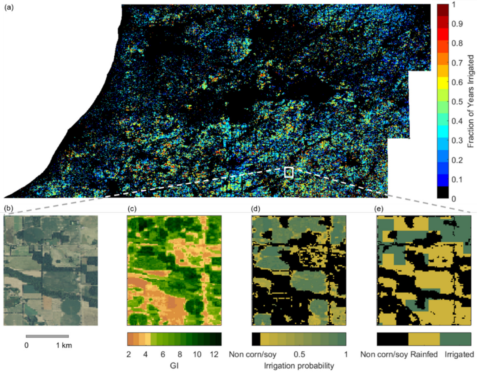
2.4. Random Forest Classifier

We use a random forest (RF) machine learning algorithm to inductively build a classifier of irrigated versus rainfed areas. We selected RF because the algorithm was successful in various hydrologic and remote sensing applications (e.g., [13,14,33,34,35] is robust with relatively large number of inputs, provides input variable importance measures and probabilistic outputs [36], and is supported in the GEE cloud computing platform.

A random forest is comprised of an ensemble of decision trees. Given a set of training data $\left\{{\mathrm{x}}_{\mathrm{i}},{\mathrm{y}}_{\mathrm{i}}\right\},\mathrm{i}=1,\dots ,\mathrm{n}$, where ${\mathrm{x}}_{\mathrm{i}}$ denotes input variables, and ${\mathrm{y}}_{\mathrm{i}}$ is the corresponding output. In this study, ${\mathrm{y}}_{\mathrm{i}}$ is a categorical variable with two classes: irrigated and rainfed. The algorithm randomly draws $n$ samples with replacements from the training dataset to train a single tree. The process is repeated $\mathrm{N}$ times, resulting in a forest of $\mathrm{N}$ trees. Once trained, each tree predicts the class of a new data point, and the $\mathrm{N}$ trees may predict $\mathrm{M}$ classes. The RF algorithm outputs the percentage of trees that provide a prediction of the $\mathrm{M}$ classes. The class that receives the highest probability is the final prediction.

In the mapping process, a composite of images is created for each year as input data layers (Table 1 and Table 2, Table S2, Supplementary Material). For each year since 2007, the composite is masked using the Cropland Data Layers (CDL, [22]) to keep only corn and soybean fields for this region. For years before 2007, the composite is masked using the National Land Cover Dataset (NLCD, [37]), the primary available product for the study region. The NLCD-based crop mask includes all row crop fields because NLCD does not distinguish among row crops. The trained RF classifier is then applied to input composites and labels each pixel as either irrigated or rainfed. In this way, we develop irrigation probability maps for every year from 2001 to 2016. The probability value ranges from 0 to 1, with higher values suggesting larger likelihood of irrigation activity in the pixel. A pixel is classified as irrigated if it receives a probability greater than 0.5, and as rainfed otherwise. The resulting binary maps are postprocessed in two steps. Due to cloud coverage, 2014 and 2015 have 8.2% and 5.7% pixels, respectively, with no Landsat scene from June 10th to August 5th. The gap pixels in 2014 are labeled irrigated if it was classified as irrigated in both 2012 and 2013. Similarly, the gap pixels in 2015 are labeled irrigated if it is classified as irrigated in the 2013 map and gap-filled 2014 map. In the second step, all pixels that are classified as irrigated only once during 2001–2015 are labeled as rainfed as it is unlikely that farmers will irrigate only one time due to high infrastructure costs. We then examine the final irrigation maps to track the spatial extent and the changing irrigation dynamics.

During training, the RF algorithm also calculates a variable importance score based on the total decrease in node impurities by splitting on the variable, averaged over all trees [38]. The variable importance scores provide a measure of the relative importance of each input variable for capturing the spatiotemporal irrigation pattern. In this study, we used all 98 input variables described in Section 2.2 and Section 2.3, and used the RF calculated variable importance measure to draw insights into the data worth of various indices in similar irrigation mapping applications. We note that RF algorithms are robust with the presence of a large number of inputs. Depending on specific applications, and especially when using other machine learning algorithms that are less robust to high input number, more sophisticated feature selection techniques (e.g., [34,39]) can be used to constrain the input space dimension.

2.5. Manually Labeled Dataset

The RF classifier is built based on a training dataset compiled from high-resolution aerial photography that was acquired during growing seasons (National Agriculture Imagery Program, NAIP [40]) from the study area. Approximately half of the training points are sampled in two representative years, 2012 and 2014. 2012 is known as a dry year in which limited rainfall induced water stress during the crop growth period. We expect that the irrigated crops are more productive than rainfed crops in this year, and the difference should be reflected in our selected indices. Therefore, 2012 represents an “easy” irrigation mapping case for the classifier. On the other hand, the 2014 growing season receives plenty of precipitation and thus represents a challenging case for the algorithm. In addition, we sampled 100 locations across multiple years (2005, 2006, 2009, 2010) to track shifts between rainfed and irrigated fields. The locations of the data points were randomly sampled after applying an agriculture land cover mask. From 2001 to 2006 the mask is derived from the NLCD and included pixels categorized as cultivated crops. Since 2007 when CDL was first available in the study area, the masks include pixels labeled as corn and soybean fields in CDL.

Through the GEE cloud computing platform, we manually labeled each point as either irrigated or rainfed based on multiple lines of evidence, including the presence of visible irrigation infrastructure, high vegetation indices, and limited water supply from remote sensing and climate data. The presence of irrigation infrastructure, primarily central pivot irrigation systems, is identified from NAIP images. When such infrastructure is identified, we examine the time series of vegetation indices, NDWI, precipitation, and NLDAS-Noah root zone soil water content to estimate whether a particular location is irrigated. As described previously, the vegetation indices and NDWI are derived from available Landsat scenes, with precipitation data from PRISM. A data point is discarded when a decision cannot be made. In total, the manually labeled dataset include 1536 data points (locations in Figure 2).

2.6. Classification Accuracy Assessment

We evaluated the accuracy of irrigation mapping using two validation data sources. First, we randomly divided the manually labeled dataset into training (80%) and validation (20%). We trained a random forest on the training dataset, and then tested its performance on the validation data points. To reduce the effects of random sampling, we repeated this sample-and-train process 20 times. We note that some of the remote sensing and climate information are used both in the manual labeling of the validation dataset as well as inputs to the random forest classifier. Such overlap may favorably influence classifier performance evaluation on the manually labeled validation dataset. However, the manually labeled reference dataset primarily relies upon visual cues in the NAIP high-resolution imagery, which was not included in the RF classification. Overlapping datasets provided only supporting evidence for manual labeling. Therefore, the validation points still provide valuable insights into irrigation mapping accuracy, especially given the lack of ground truth data. As a second, independent assessment, we calculated the total irrigated area of corn and soybean for each county in the study domain. The results are compared with county-wise statistics of the two crops available through NASS Agricultural Census [2] in the available years (2002, 2007, 2012).

For comparison, we also evaluate the accuracy of MIrAD-US, a national, 250-m resolution irrigation dataset available in 2002, 2007 and 2012 [12], using the manually labeled dataset. The MIrAD-US product identifies irrigated pixels when MODIS annual peak NDVI exceeds a threshold, which is adjusted for each county such that the resulting total irrigated acreage agrees with the USDA NASS statistics. We compare MIrAD-US label (irrigated versus rainfed) with the manually labeled dataset (Section 2.5), with error rates reported in Section 3.1. The MIrAD-US error rate is then compared with RF classification validation error for data points in 2012 (no training data is generated in 2002 and 2007 due to lack of NAIP images), averaged over 20 repeated experiments.

3. Results and Discussions

We developed annual irrigation probability maps for 2001 to 2016 (Figure 3) by integrating Landsat remote sensing imagery and hydroclimatic variables in a RF analysis as discussed above. Figure 3 shows the irrigation probability maps for a 2.7 by 3.2 km area in 2012. Comparing the irrigation maps with NAIP imagery (Figure 3b,c), the RF classifier can identify irrigation with detailed sub-field spatial pattern, which national products such as MIrAD-US cannot capture due to its coarse resolution (Figure 3e). This is important, as small fragmented fields are common in the study area. It is important to note that NAIP imagery was only used to label training points and not included in the input data to produce the irrigation maps. Figure 3c shows the green indices calculated from the Landsat scene that immediately follows a dry period (GI_ppt), which is identified as the longest consecutive days with daily precipitation less than 5 mm (Section 2.4). This variable is the most important input variable according to RF important score (see Section 3.2 for more details).

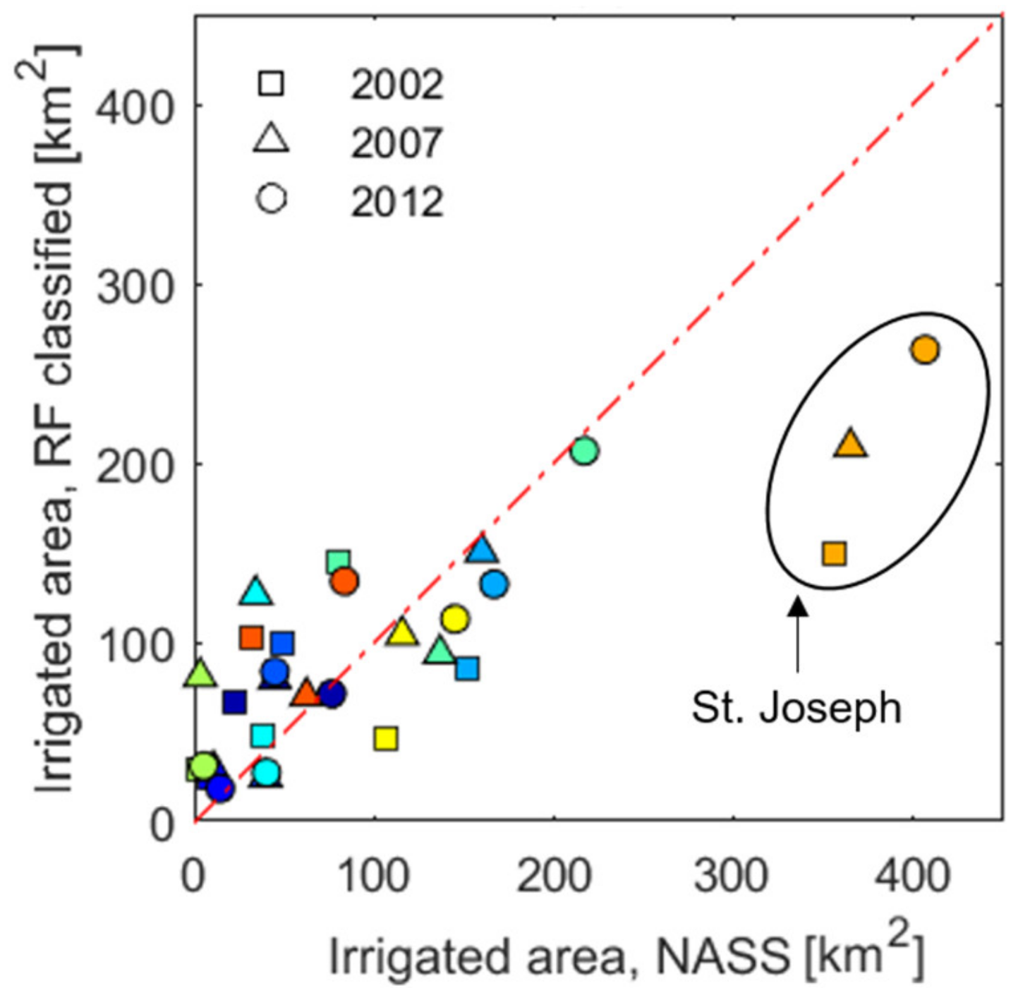
3.1. Classification Accuracy

First, we examined the error rate of the RF classifier on the validation points we reserved before training the classifier, as described in Section 2.5. Accuracies for all years, dry years (6/15 to 7/31 precip. < 2001–2016 mean), and wet years (6/15 to 7/31 precip. > 2001–2016 mean) are 82%, 85% and 78%, respectively (

Table 3. Irrigation mapping accuracy evaluated using manually labeled data points. Omission error describes the percentage of irrigated training points that are classified as rainfed (false negative), while commission error describes the percentage of rainfed training points that were classified as irrigated (false positive). The accuracies of RF classifier and MIrAD-US [12] are compared for 2012 when both the manually labeled data points and MIrAD-US map are available.

Year	Omission Error	Commission Error	Overall Accuracy
Dry (2009, 2012)	40%	9%	85%
Wet (2005, 2006, 2010, 2014)	38%	14%	78%
All years	39%	13%	82%
2012 RF (This study)	39%	6%	84%
2012 MIrAD-US [12]	49%	16%	74%

). It is not surprising that the classification accuracy is lower in wet years that received plenty of precipitation. In wet years, the input indices describing the crop status may not be significantly different between rainfed and irrigated fields, inducing higher commission error and lower omission error than in dry years (Table 3). It is notable that the difference between the accuracies in dry and wet years is small. This suggests the utility of spatial anomaly and weather-sensitive remote sensing indices in distinguishing irrigated fields from rainfed even under humid conditions.

We then compared the county irrigated area classified by RF with NASS Agricultural Census statistics [2] in 2002, 2007, 2012, as shown in Figure 4. For county statistics, there is a good overall agreement $\left(r^2=0.69\right)$. Figure 5 reports the annual total irrigated area in the study domain. While spread is noticeable in the county data (Figure 4), the total irrigated area agrees well with NASS statistics.

Next, we compared the error rate of RF classifier and MIrAD-US using the manually labeled data (Section 2.5 and Section 2.6) in 2012 when both the manually labeled data points and MIrAD-US map are available. As shown in Table 3, the MIrAD-US error rate (defined as 1—accuracy) is 26%, and the RF classifier error rate is 16%. In addition, RF irrigation maps have lower omission and commission errors than MIrAD-US, suggesting a higher accuracy of RF-derived irrigation maps.

The high omission error of the irrigation classification (Table 3) may be due to the agricultural management practice of deficit irrigation in the study area. Notably from Figure 4, the RF classifier significantly underestimated irrigated area in St. Joseph county where seed corn is the dominant crop [18], and deficit irrigation in late season (August) is commonly applied to dry up corn in plots. These locations would thus exhibit lower vegetation indices. The irrigation maps may underrepresent locations where a deficit irrigation strategy is applied in the rest part of the study domain.

The accuracy assessed on the validation points is lower than previous study that used a similar method to map irrigated area in a semi-arid to arid region [13]. In a more arid climate, the vegetation indices of rainfed crops are distinctively lower than those of irrigated crops. This is not the case in humid to subhumid climates. As shown in Figure 5, while the mean value of GI_ppt is higher in irrigated fields, the distributions of the two classes largely overlap. Such mixing also occurs for other input variables, making separation of the two classes challenging in humid regions.

The accuracy of our irrigation maps is also subject to the uncertainties of the input data. As described in Section 2.2, the irrigation maps are developed based on crop masks derived from NLCD and CDL. Thus, misclassification of either product affects the validity of training points and the accuracy of irrigation maps. For years before 2007, the crop mask based on NLCD includes all row crop fields, thus the classified irrigated fields likely include irrigated fields other than corn and soybean. Furthermore, cloud coverage inevitably leads to missing scenes during the critical crop development phase. For locations with few available Landsat scenes, important information regarding the crop status may be missing, and resulting classification may be misled. The issue of cloud coverage may be alleviated using fusion of remote sensing products across recent platforms [41,42] such as radar imagery [15]. Finally, fields smaller than the 30-m resolution may not be well captured by the Landsat-based mapping method.

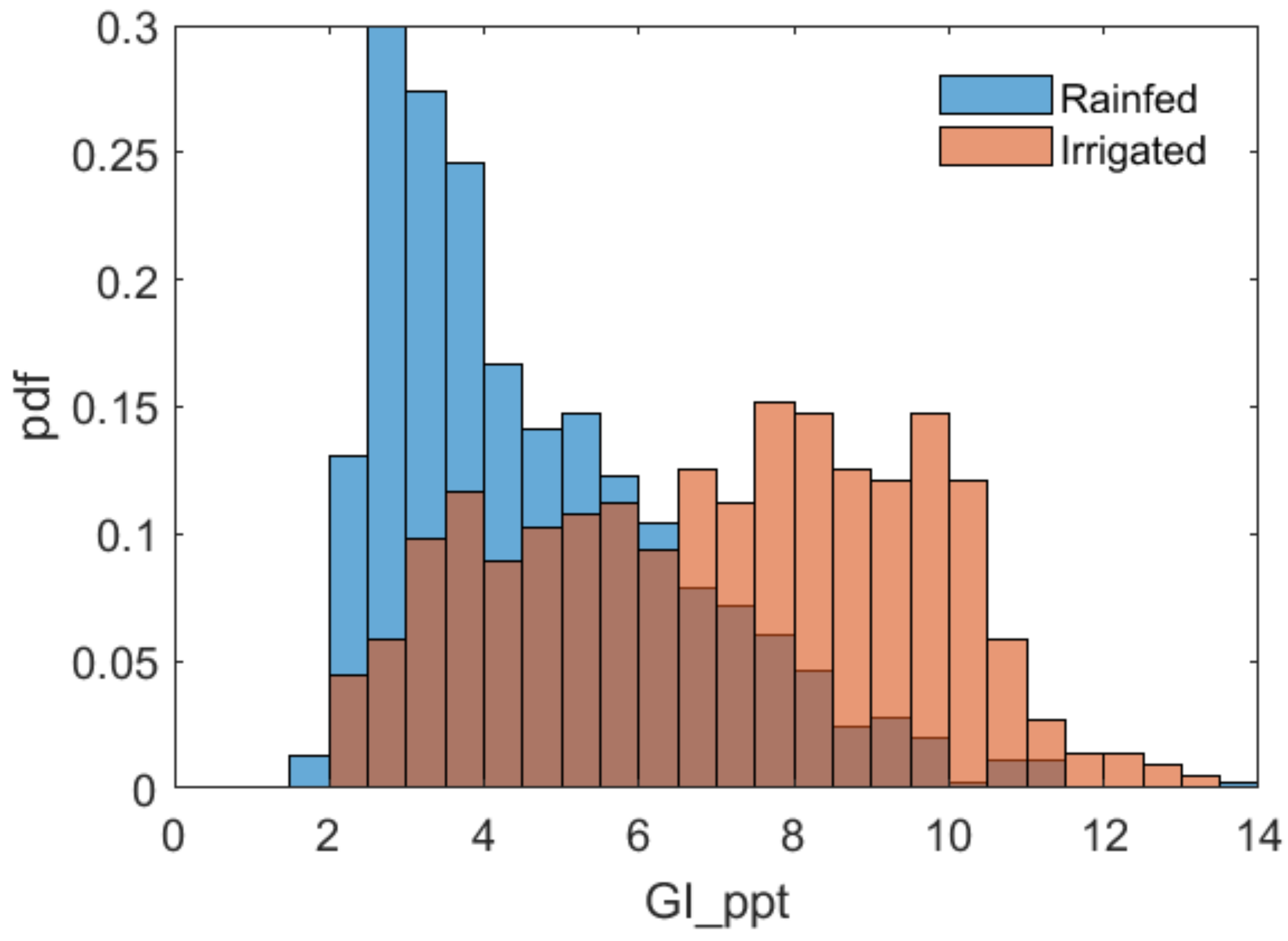
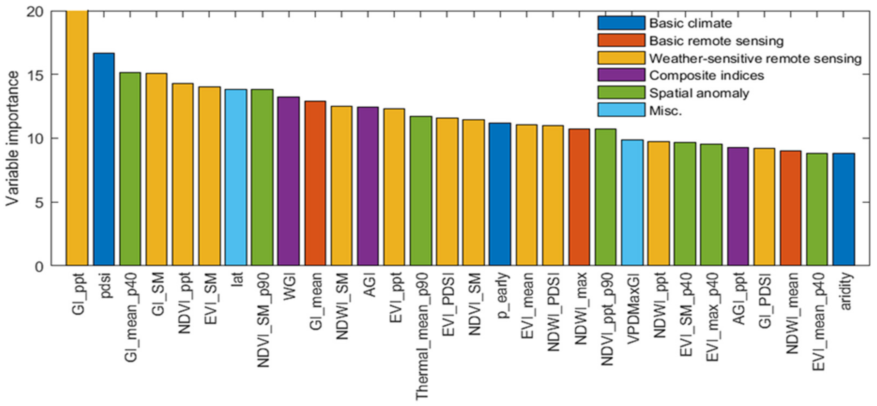
3.2. Important Input Variables

During the training process, the RF classifier calculates the variable importance scores as how much impurity (i.e., irrigated versus rainfed) can be explained by each input variable. Figure 6 depicts the 30 variables receiving the highest scores. Most of these higher-ranking variables are weather-sensitive remote sensing indices from Landsat scenes immediately following a dry period identified by low soil water content, negative PDSI, or limited precipitation. This finding highlights the importance of selecting Landsat scenes that provide the most information for separating irrigated fields from rainfed ones. These critical scenes capture crop performance under a water stress condition; irrigated crops are expected to exhibit higher vegetation indices than rainfed crops. Such differences are not captured by peak vegetation indices, as rainfed crops may exhibit vegetation indices as high as irrigated crops during periods with sufficient precipitation. Simple remote sensing indices such as peak vegetation indices are not among the variables that explain most of irrigation spatiotemporal variability. In humid regions, maximum vegetation indices can be biased due to extensive cloud coverage.

Composites and some spatial anomaly indices receive high importance score, suggesting the utility of these variables to identify irrigated fields. Besides climate and remote sensing data, latitude is among the most important variables, likely due to the gradient of increasing fraction of seed corn from north to south. It is common to regularly irrigate seed corn as required in contracts. In addition, water supply indicators such as PDSI and pre-season precipitation (p_early) receive high ranks because they can explain the interannual climate variability. Other climate variables received lower importance scores.

We found that soil properties and slope are not important factors for simulating the spatial distribution of irrigation in this region. This is not surprising because sandy soil with low AWC and mild terrain are prevalent in the agricultural lands of the study area. Other variables that do not appear to be important include soil water content, precipitation, aridity and extreme weather condition indices such as GDD, dryspell and heatwave, likely because the resolution of the meteorological data used to calculate these indices is too coarse to capture the fine-scale heterogeneity of irrigation. However, these variables portray large-scale water supply and demand, and we have shown that they can be used to select Landsat scenes that provide the best information for separating irrigated fields from rainfed ones. In particular, soil water content is simulated by NLDAS-Noah, which does not account for irrigation and estimates wetness under rainfed conditions.

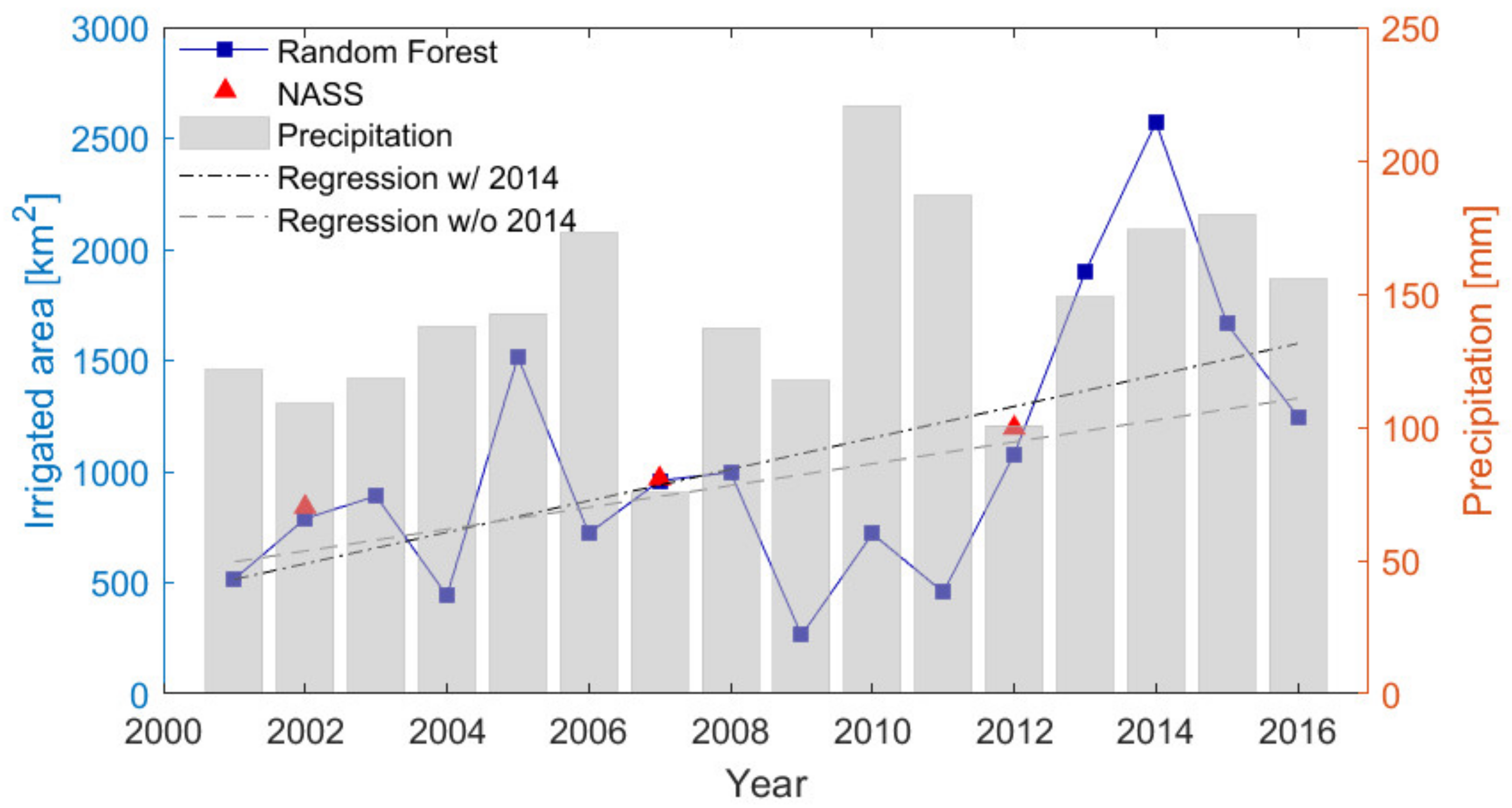
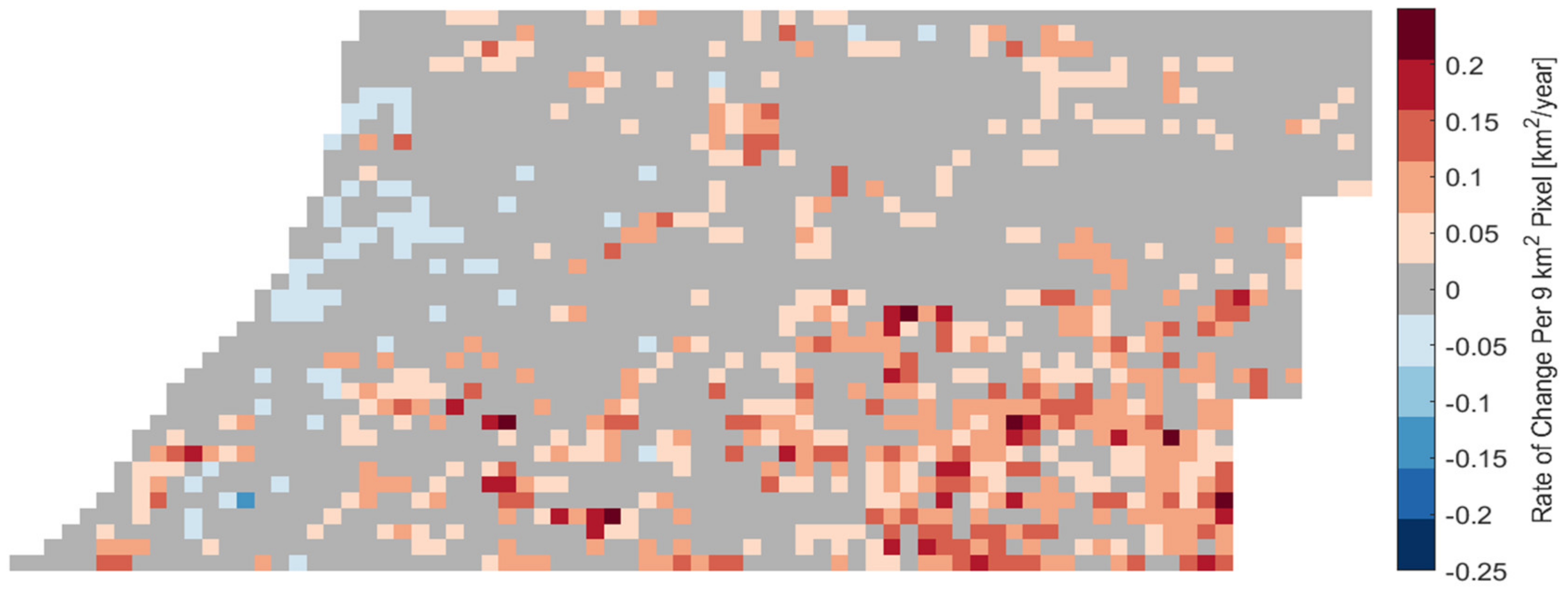
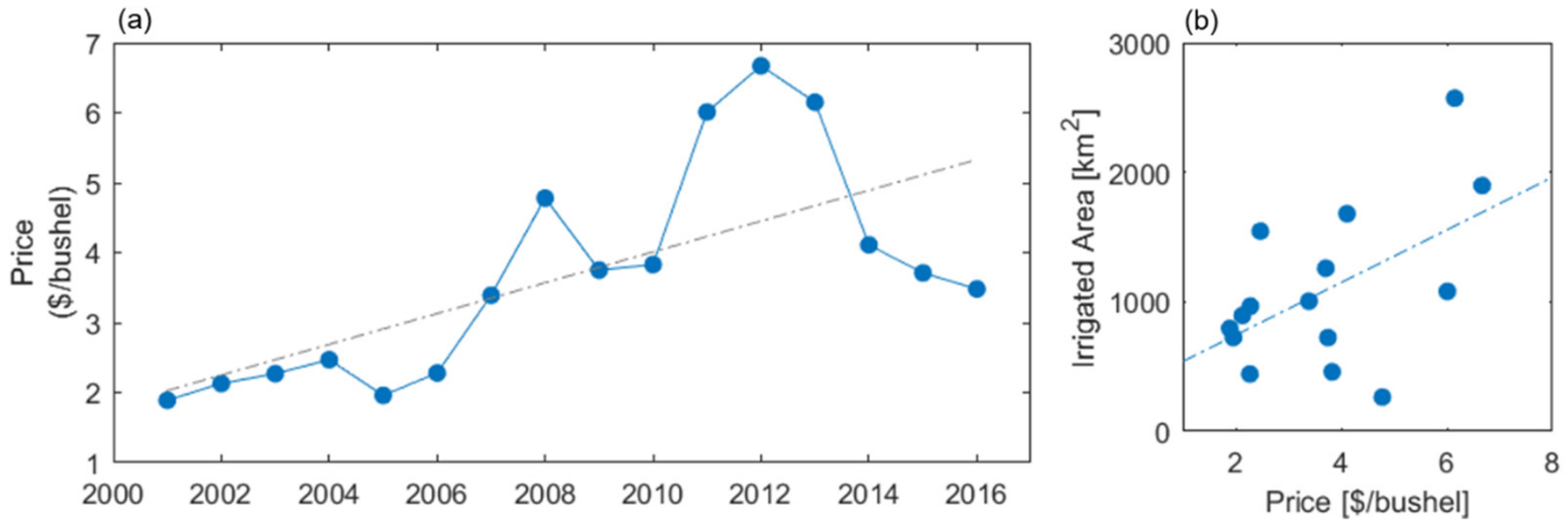
3.3. Expansion of Irrigation

From the RF classified irrigation maps we calculated the total irrigated area for the study region for 2001–2016 (Figure 7) and compared this to NASS statistics. Temporal fluctuation is noticeable, with limited irrigated area in 2009–2011 and high irrigated area in 2013–2014. The peak in 2014 is likely a combination of three factors. First, the critical crop development phase in 2014 had 21% higher than average (Figure 7) and more frequent precipitation (the dryspell of the study area is 13 days in 2014 and 17 averaged over 2001–2016), leading to robust rainfed crops and correspondingly high vegetation index values across the region. Thus, the RF classifier may overestimate the irrigated area in this year. Second, as described in Section 2.5, 2014 has 8.2% pixels with no Landsat scenes during the critical crop development phase. To fill in the gaps, we labeled pixels as irrigated in 2014 if they were classified as irrigated in both 2012 and 2013. This may result in commission errors (i.e., classifying rainfed fields as irrigated) in those pixels. Third, farmers may have switched to irrigated agriculture after the crop losses in the 2012 drought.

There is a statistically significant ($p$ < 0.05) increasing trend in irrigation in this study region despite notable interannual variability. Over the 16-year period, irrigated area tripled (increased by 204%), according to the linear regression shown in Figure 7. The estimated slope of 70.8 km²/year is approximately twice the estimate from NASS statistics in 2002, 2007 and 2012 (slope = 35.6 km²/year). In order to isolate the likely skewness due to high irrigated area estimated in 2014, we performed another linear regression excluding 2014 (Figure 7). An increasing trend is statistically significant ($p$ < 0.05) with estimated slope of 49.1 km²/year.

We also calculated the change in irrigated area for corn and soybeans, respectively, for 2007–2016, when CDL is available for the study area. The irrigated area fractions for corn and soybeans increased from 19.1% in 2007 to 24.9% in 2016, and from 9.2% in 2007 to 17.9% in 2016, respectively.

To examine the spatial pattern, irrigation trends are calculated based on linear regression (Figure 8). To do this, we aggregated the 30-m irrigation maps to a larger grid to perform linear regression on the irrigated area through time. We chose the 9-km² grid to examine relatively fine-scale spatial patterns of irrigation trends across the region (vs. county level, for instance). Slight decreasing trends in lakeshore area suggests discontinuation of irrigation. The highest increase rate (up to 0.25 km²/year per 9-km² cell) was found in southern part of the study area. The irrigation expansion is believed to be associated with the promotion of seed corn in this area [16,18]. Seed corn is usually irrigated because irrigation is typically required by the contracts between farmers and seed corn companies.

In addition, correlation analyses suggest crop commodity price is another factor affecting irrigation decisions. The annual irrigated area of the study region is found to be correlated with previous year’s corn price [2] (Figure 9, $r$ = 0.66, $p$ = 0.009). Irrigation may double corn yields and increase soybean yields by more than 66% in SW MI [16]. Given the easy accessibility to irrigation water, adoption of irrigation will likely increase farmers’ revenue. Irrigation expansion may be further encouraged by devastating crop losses in the 2012 drought in fields without irrigation [43,44].

4. Conclusions

By integrating satellite imagery and hydroclimatic information using a machine learning algorithm, we created annual irrigation maps for a subhumid area in southwestern Michigan for 2001–2016. The maps capture the spatiotemporal pattern of irrigation at a high spatial resolution (30 m) and indicate that irrigated area in southwestern Michigan roughly tripled in the last 16 years according to linear regression.

We demonstrated the utility of novel input variables including weather-sensitive remote sensing, spatial anomalies, and recently-developed composite indices. In particular, we found that those vegetation indices following dry periods are the most important to distinguish irrigated fields from rainfed. This not only reduces the number of scenes (thus memory and computational expense) to process, but also avoids possible confounding effects of high vegetation indices captured during a wet period.

The annual irrigation maps are validated using multiple data sources. Reasonable accuracy is achieved despite the difficulties involved with estimating irrigated area in a region with a subhumid climate and heterogeneous agricultural management practices (e.g., deficit irrigation strategy for seed corn). We found that the mapping accuracy in dry years is higher than in wet years with a narrow margin. The small difference between accuracies may be attributed to the use of spatial anomaly and weather-sensitive remote sensing indices, which were able to distinguish irrigated from rainfed fields even under subhumid conditions.

We identified several challenges and limitations for mapping irrigated areas in subhumid to humid regions, including the dependency on the quality of input data (e.g., land cover) and cloud coverage, which is more frequent in such regions. The substantial efforts and difficulty involved in generating training data are also noteworthy and call for in season high-resolution imagery. Nevertheless, the promising results underscore the potential of using remote sensing and cloud computing to provide valuable information for water resources decision makers and hydrologic studies at regional scales.

References

1. Food and Agriculture Organization of the United Nations (FAO) AQUASTAT Main Database. Available online: http://www.fao.org/nr/aquastat (accessed on 1 January 2016).
2. U.S Department of Agriculture. National Agricultural Statistics Service (USDA NASS) QuickStats Ad-hoc Query Tool. Available online: https://quickstats.nass.usda.gov/ (accessed on 1 November 2017).
3. Cotterman, K.A.; Kendall, A.D.; Basso, B.; Hyndman, D.W. Groundwater depletion and climate change: Future prospects of crop production in the Central High Plains Aquifer. Clim. Change 2018, 146, 187–200. [Google Scholar] [CrossRef]
4. Pei, L.; Moore, N.; Zhong, S.; Luo, L.; Hyndman, D.W.; Heilman, W.E.; Gao, Z. WRF Model Sensitivity to Land Surface Model and Cumulus Parameterization under Short-Term Climate Extremes over the Southern Great Plains of the United States. J. Clim. 2014, 27, 7703–7724. [Google Scholar] [CrossRef]
5. Pei, L.; Moore, N.; Zhong, S.; Kendall, A.D.; Gao, Z.; Hyndman, D.W. Effects of Irrigation on Summer Precipitation over the United States. J. Clim. 2016, 29, 3541–3558. [Google Scholar] [CrossRef]
6. Smidt, S.J.; Haacker, E.M.K.; Kendall, A.D.; Deines, J.M.; Pei, L.; Cotterman, K.A.; Li, H.; Liu, X.; Basso, B.; Hyndman, D.W. Complex water management in modern agriculture: Trends in the water-energy-food nexus over the High Plains Aquifer. Sci. Total Environ. 2016, 566–567, 988–1001. [Google Scholar] [CrossRef] [PubMed]
7. Kumar, S.V.; Peters-Lidard, C.D.; Santanello, J.A.; Reichle, R.H.; Draper, C.S.; Koster, R.D.; Nearing, G.; Jasinski, M.F. Evaluating the utility of satellite soil moisture retrievals over irrigated areas and the ability of land data assimilation methods to correct for unmodeled processes. Hydrol. Earth Syst. Sci. 2015, 12, 5967–6009. [Google Scholar] [CrossRef]
8. Lawston, P.M.; Santanello, J.A.; Franz, T.E.; Rodell, M. Assessment of irrigation physics in a land surface modeling framework using non-traditional and human-practice datasets. Hydrol. Earth Syst. Sci. 2017, 21, 2953–2966. [Google Scholar] [CrossRef] [PubMed] [Green Version]
9. McInerney, D.; Thyer, M.; Kavetski, D.; Githui, F.; Thayalakumaran, T.; Liu, M.; Kuczera, G. The Importance of Spatiotemporal Variability in Irrigation Inputs for Hydrological Modeling of Irrigated Catchments. Water Resour. Res. 2018, 54, 6792–6821. [Google Scholar] [CrossRef]
10. Levin, S.B.; Zarriello, P.J. USGS Scientific Investigations Report 2013–5066: Estimating Irrigation Water Use in the Humid Eastern United States; USGS: Reston, VA, USA, 2013. [Google Scholar]
11. Pervez, M.S.; Brown, J.F. Mapping irrigated lands at 250-m scale by merging MODIS data and National Agricultural Statistics. Remote Sens. 2010, 2, 2388–2412. [Google Scholar] [CrossRef]
12. Brown, J.F.; Pervez, M.S. Variability and trends in irrigated and non-irrigated croplands in the central U.S. In Proceedings of the 2013 Second International Conference on Agro-Geoinformatics (Agro-Geoinformatics); IEEE, Fairfax, VA, USA, 12–16 August 2013; pp. 102–105. [Google Scholar]
13. Deines, J.M.; Kendall, A.D.; Hyndman, D.W. Annual Irrigation Dynamics in the U.S. Northern High Plains Derived from Landsat Satellite Data. Geophys. Res. Lett. 2017, 44, 9350–9360. [Google Scholar] [CrossRef]
14. Deines, J.M.; Kendall, A.D.; Butler, J.J.; Hyndman, D.W. Quantifying water use and farmer adaptation strategies in response to novel stakeholder-driven groundwater management in teh US High Plains Aquifer. Environ. Res. Lett. 2019. [CrossRef]
15. Gao, Q.; Zribi, M.; Escorihuela, M.; Baghdadi, N.; Segui, P.; Gao, Q.; Zribi, M.; Escorihuela, M.J.; Baghdadi, N.; Segui, P.Q. Irrigation Mapping Using Sentinel-1 Time Series at Field Scale. Remote Sens. 2018, 10, 1495. [Google Scholar] [CrossRef]
16. Michigan State University (MSU) Extension. Value of Irrigation to the Southwest Michigan Economy; MSU: Lansing, MI, USA, 2014. [Google Scholar]
17. USDA Natural Resources Conservation Service (NRCS) Web Soil Survey. Available online: https://websoilsurvey.nrcs.usda.gov/ (accessed on 1 November 2017).
18. Kaercher, M.; Neumann, B. St. Joseph County Agriculture: Past, Present and Future; MSU: Centreville, MI, USA, 2006. [Google Scholar]
19. Kraft, G.J.; Clancy, K.; Mechenich, D.J.; Haucke, J. Irrigation Effects in the Northern Lake States: Wisconsin Central Sands Revisited. Ground Water 2012, 50, 308–318. [Google Scholar] [CrossRef] [PubMed]
20. Wolock, D.M.; Winter, T.C.; McMahon, G. Delineation and Evaluation of Hydrologic-Landscape Regions in the United States Using Geographic Information System Tools and Multivariate Statistical Analyses. Environ. Manag. 2004, 34, S71–S88. [Google Scholar] [CrossRef] [PubMed]
21. Daly, C.; Halbleib, M.; Smith, J.I.; Gibson, W.P.; Doggett, M.K.; Taylor, G.H.; Curtis, J.; Pasteris, P.P. Physiographically sensitive mapping of climatological temperature and precipitation across the conterminous United States. Int. J. Climatol. 2008, 28, 2031–2064. [Google Scholar] [CrossRef] [Green Version]
22. U.S. Department of Agriculture. National Agricultural Statistics Service (USDA NASS) Cropland Data Layer. Available online: https://www.nass.usda.gov/Research_and_Science/Cropland/Release/index.php (accessed on 1 April 2018).
23. Gorelick, N.; Hancher, M.; Dixon, M.; Ilyushchenko, S.; Thau, D.; Moore, R. Google Earth Engine: Planetary-scale geospatial analysis for everyone. Remote Sens. Environ. 2017, 202, 18–27. [Google Scholar] [CrossRef]
24. USGS 1 Arc-second Digital Elevation Models (DEMs)—USGS National Map 3DEP Downloadable Data Collection. Available online: https://www.sciencebase.gov/catalog/item/4f70aa71e4b058caae3f8de1 (accessed on 1 November 2017).
25. Schaap, M.G.; Leij, F.J.; van Genuchten, M.T. ROSETTA: A computer program for estimating soil hydraulic parameters with hierarchical pedotransfer functions. J. Hydrol. 2001, 251, 163–176. [Google Scholar] [CrossRef]
26. Abatzoglou, J.T. Development of gridded surface meteorological data for ecological applications and modelling. Int. J. Climatol. 2013, 33, 121–131. [Google Scholar] [CrossRef]
27. Xia, Y.; Mitchell, K.; Ek, M.; Sheffield, J.; Cosgrove, B.; Wood, E.; Luo, L.; Alonge, C.; Wei, H.; Meng, J.; et al. Continental-scale water and energy flux analysis and validation for the North American Land Data Assimilation System project phase 2 (NLDAS-2): 1. Intercomparison and application of model products. J. Geophys. Res. Atmos. 2012, 117. [Google Scholar] [CrossRef] [Green Version]
28. White, J.C.; Wulder, M.A.; Hobart, G.W.; Luther, J.E.; Hermosilla, T.; Griffiths, P.; Coops, N.C.; Hall, R.J.; Hostert, P.; Dyk, A.; et al. Pixel-Based Image Compositing for Large-Area Dense Time Series Applications and Science. Can. J. Remote Sens. 2014, 40, 192–212. [Google Scholar] [CrossRef] [Green Version]
29. Gao, B. NDWI—A normalized difference water index for remote sensing of vegetation liquid water from space. Remote Sens. Environ. 1996, 58, 257–266. [Google Scholar] [CrossRef]
30. Ozdogan, M.; Gutman, G. A new methodology to map irrigated areas using multi-temporal MODIS and ancillary data: An application example in the continental US. Remote Sens. Environ. 2008, 112, 3520–3537. [Google Scholar] [CrossRef] [Green Version]
31. Running, S.; Mu, Q.; Zhao, M.; Moreno, A. MODIS Global Terrestrial Evapotranspiration (ET) Product (NASA MOD16A2/A3) Collection 5; NASA Headquarters: Washington, DC, USA, 2013. [Google Scholar]
32. McAllister, A.; Whitfield, D.; Abuzar, M. Mapping Irrigated Farmlands Using Vegetation and Thermal Thresholds Derived from Landsat and ASTER Data in an Irrigation District of Australia. Photogramm. Eng. Remote Sens. 2015, 81, 229–238. [Google Scholar] [CrossRef]
33. Naghibi, S.A.; Pourghasemi, H.R.; Dixon, B. GIS-based groundwater potential mapping using boosted regression tree, classification and regression tree, and random forest machine learning models in Iran. Environ. Monit. Assess. 2016, 188, 44. [Google Scholar] [CrossRef] [PubMed]
34. Xu, T.; Valocchi, A.J. Data-driven methods to improve baseflow prediction of a regional groundwater model. Comput. Geosci. 2015, 85, 124–136. [Google Scholar] [CrossRef]
35. Xu, T.; Valocchi, A.J.; Ye, M.; Liang, F.; Lin, Y.F. Bayesian calibration of groundwater models with input data uncertainty. Water Resour. Res. 2017, 53, 3224–3245. [Google Scholar] [CrossRef]
36. Breiman, L. Random Forests. Mach. Learn. 2001, 45, 5–32. [Google Scholar] [CrossRef] [Green Version]
37. Fry, J.; Xian, G.Z.; Jin, S.; Dewitz, J.; Homer, C.G.; Yang, L.; Barnes, C.A.; Herold, N.D.; Wickham, J.D. Completion of the 2006 national land cover database for the conterminous united states. Photogramm. Eng. Remote Sens. 2011, 77, 858–864. [Google Scholar]
38. Hastie, T.; Friedman, J.; Tibshirani, R. The Elements of Statistical Learning; Springer: New York, NY, USA, 2001. [Google Scholar]
39. Abe, S. Feature Selection and Extraction; Springer: London, UK, 2010; pp. 331–341. [Google Scholar]
40. National Agriculture Imagery Program (NAIP) USDA Farm Service Agency National Agriculture Imagery Program. Available online: https://www.fsa.usda.gov/programs-and-services/aerial-photography/imagery-programs/naip-imagery/ (accessed on 1 November 2017).
41. Boschetti, L.; Roy, D.P.; Justice, C.O.; Humber, M.L. MODIS–Landsat fusion for large area 30 m burned area mapping. Remote Sens. Environ. 2015, 161, 27–42. [Google Scholar] [CrossRef]
42. Wang, Q.; Blackburn, G.A.; Onojeghuo, A.O.; Dash, J.; Zhou, L.; Zhang, Y.; Atkinson, P.M. Fusion of Landsat 8 OLI and Sentinel-2 MSI Data. IEEE Trans. Geosci. Remote Sens. 2017, 55, 3885–3899. [Google Scholar] [CrossRef]
43. Boyer, J.S.; Byrne, P.; Cassman, K.G.; Cooper, M.; Delmer, D.; Greene, T.; Gruis, F.; Habben, J.; Hausmann, N.; Kenny, N.; et al. The U.S. drought of 2012 in perspective: A call to action. Glob. Food Sec. 2013, 2, 139–143. [Google Scholar] [CrossRef]
44. Zhang, T.; Lin, X.; Sassenrath, G.F. Current irrigation practices in the central United States reduce drought and extreme heat impacts for maize and soybean, but not for wheat. Sci. Total Environ. 2015, 508, 331–342. [Google Scholar] [CrossRef] [PubMed]
Figure 1. (a). The location (inset) and remotely sensed crop types (CDL, [22]) of the study area, including ten southwestern Michigan counties. (b) Precipitation from 15 June to 31 July (blue), and the remainder of year (gray) in the study area.
Remotesensing 11 00370 g001
Figure 2. Training points are randomly generated, scattered in crop areas. One-time training points (green triangles) are generated for 2012 (dry) and 2014 (wet) years. Additional points (red dots) are generated for 2005, 2006, 2009, 2010, 2012 and 2014.
Remotesensing 11 00370 g002
Figure 3. (a) Map of fraction of years classified as irrigated since earliest year irrigated according to the fandom forest (RF)-based annual irrigation maps spanning 2001–2016. For example, a pixel that is irrigated every year since the start of irrigation in 2012 will receive a fraction of 1.0. 2012 insets of (b) NAIP aerial image showing irrigated farms with varying sizes, (c) GI calculated from the Landsat scene that immediately follows the largest dryspell (GI_ppt), (d) random forest-based irrigation probability map with 30-m resolution and (e) MIrAD-US irrigation map with 250-m resolution. Images (be) are for 2012. Areas not classified as corn or soybeans (USDA-NASS, 2016) are shown in dark.
Remotesensing 11 00370 g003
Figure 4. County irrigated area for 2002, 2007, 2012 according to the RF-based irrigation maps. Color encodes different counties. As explained in Section 3.1, RF significantly underestimates irrigated area in St. Joseph county due to widespread seed corn production in that area.
Remotesensing 11 00370 g004
Figure 5. Empirical probability density function of green index following maximum dryspell (GI_ppt) estimated from manually labelled dataset.
Remotesensing 11 00370 g005
Figure 6. Top 30 (of 98) important variables as identified by RF; variables are grouped into six categories as indicated by different colors (Section 2.2 and Section 2.3, Table 1 and Table 2, Table S2, Supplementary Material).
Remotesensing 11 00370 g006
Figure 7. Annual total irrigated area in SW MI according to the random forest-based irrigation maps (line with squares), NASS Consensus (triangles, [2]). Gray bars show precipitation during the 15 June–31 July period, averaged over the study domain. Linear regression with and without 2014 irrigated area is also shown.
Remotesensing 11 00370 g007
Figure 8. Rate of change of irrigated area over time based on linear regression calculated for an aggregated 9 km 2 grid. Gray indicates non-significant trend ( α > 0.1 ).
Remotesensing 11 00370 g008
Figure 9. Commodity price of corn (a) and its correlation with irrigated area (b) 2001–2016.
Remotesensing 11 00370 g009