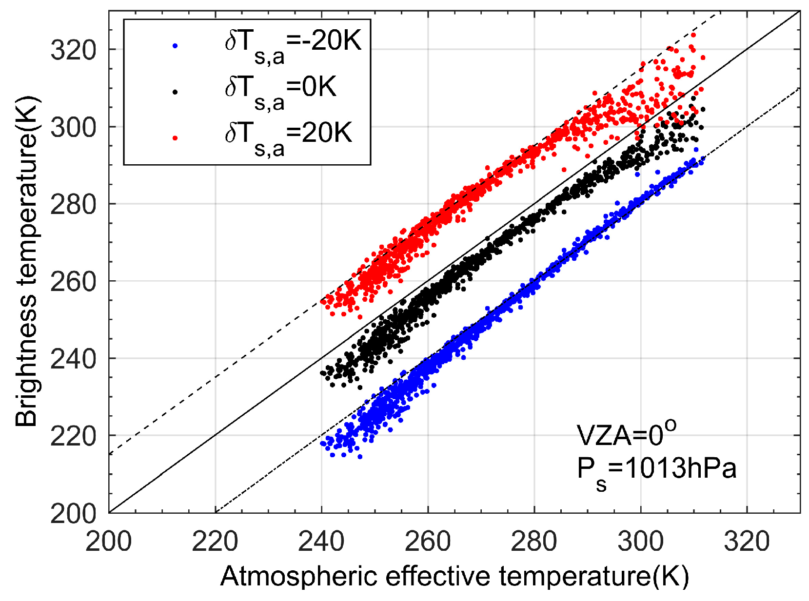
Figure 1.
Brightness temperature of Moderate Resolution Imaging Spectroradiometer (MODIS) channel 31 versus atmospheric effective temperature for various δTs,a values. Atmospheric effective temperature was defined by the DLR and atmospheric effective emissivity that was simulated using MODTRAN and 875 TIGR2002 profiles.
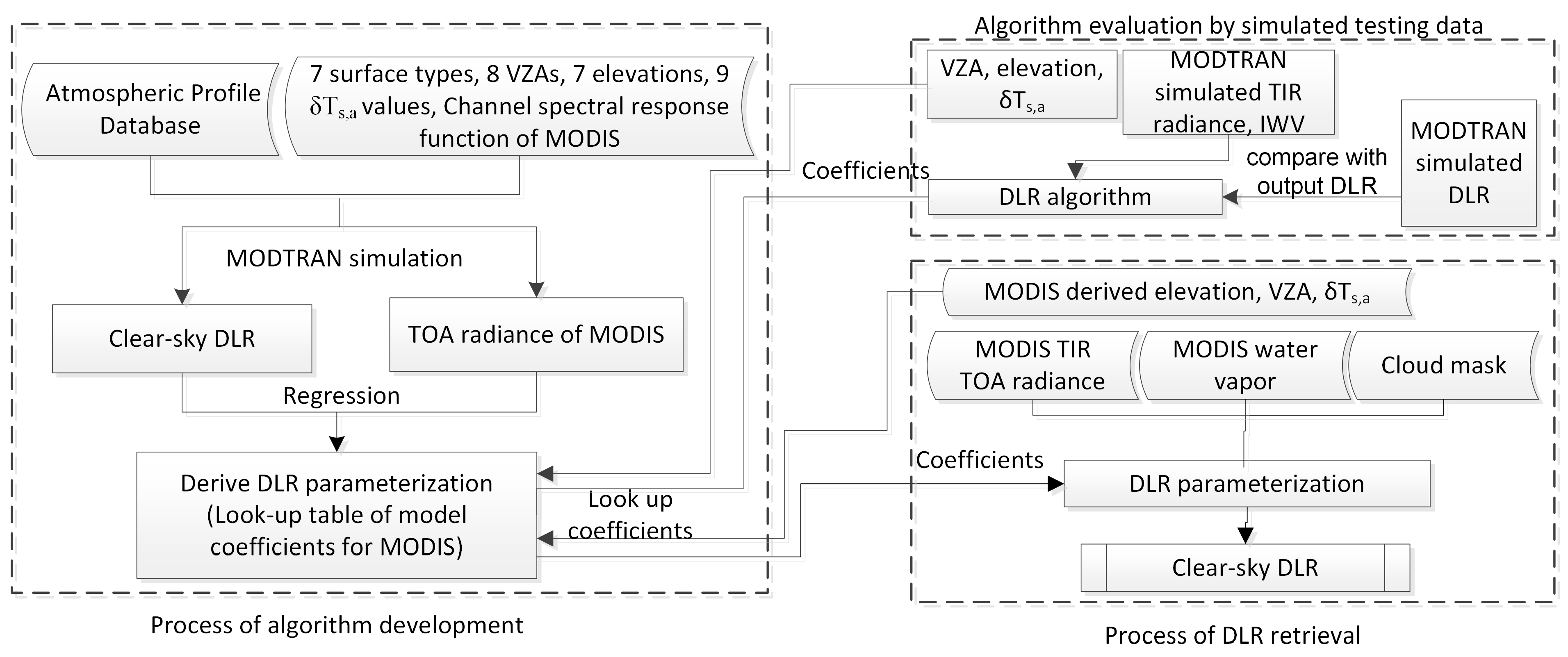
Figure 2.
Flowchart of DLR modeling process and DLR derivation.
Figure 2.
Flowchart of DLR modeling process and DLR derivation.
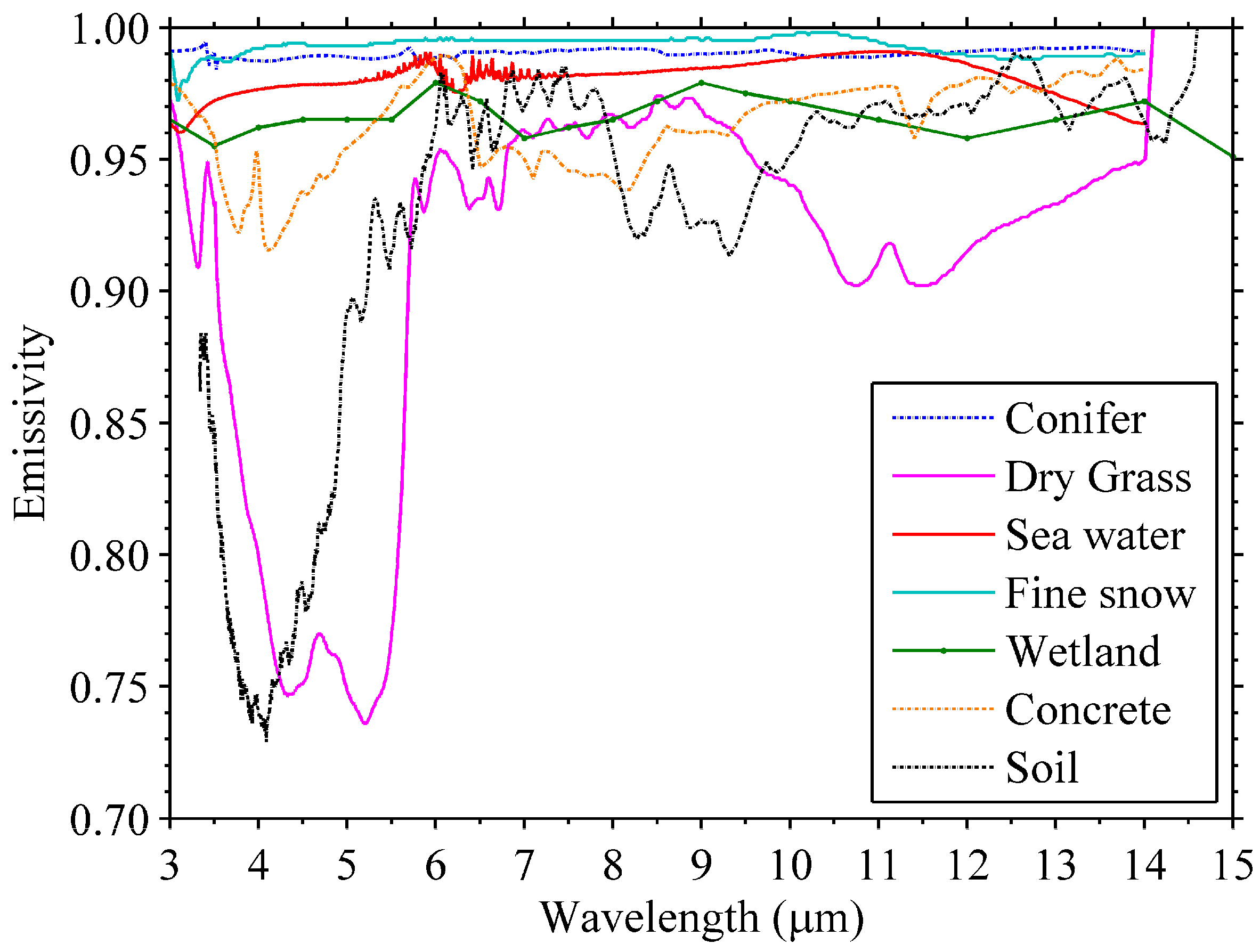
Figure 3.
Spectral emissivity curves of seven surface types from ASTER used in MODTRAN simulation.
Figure 3.
Spectral emissivity curves of seven surface types from ASTER used in MODTRAN simulation.
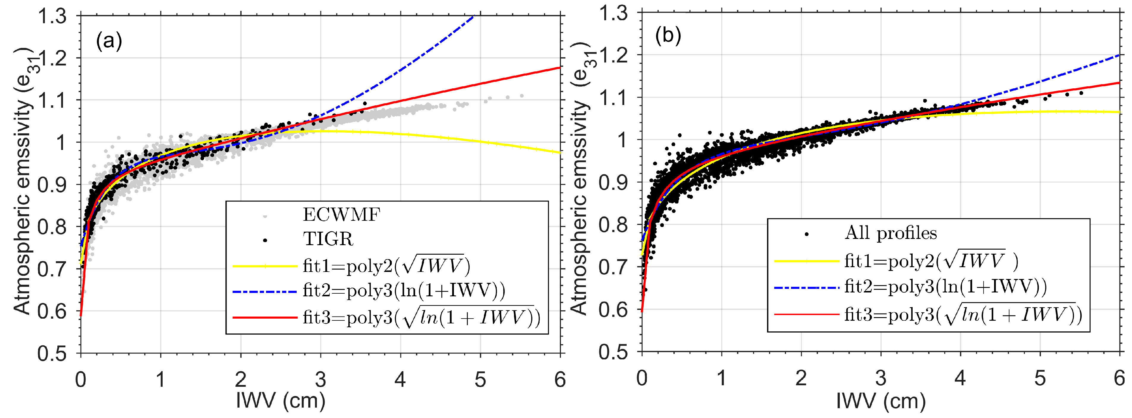
Figure 4.
Atmospheric emissivity (ε31) defined by Equation (3) using brightness temperature (BT) of MODIS 31st channel, plotted as functions of IWV at the condition of conifer surface, H = 1.435 km, view zenith angle (VZA) = 0°, and δTs,a = 0 K. The black and gray dots represent TIGR2002 and ECWMF profiles, respectively. Only the TIGR2002 profiles were used in regression in Figure (a), and all the TIGR2002 and the ECWMF profiles were used in Figure (b). Poly2 and poly3 represent quadratic and cubic function, respectively.
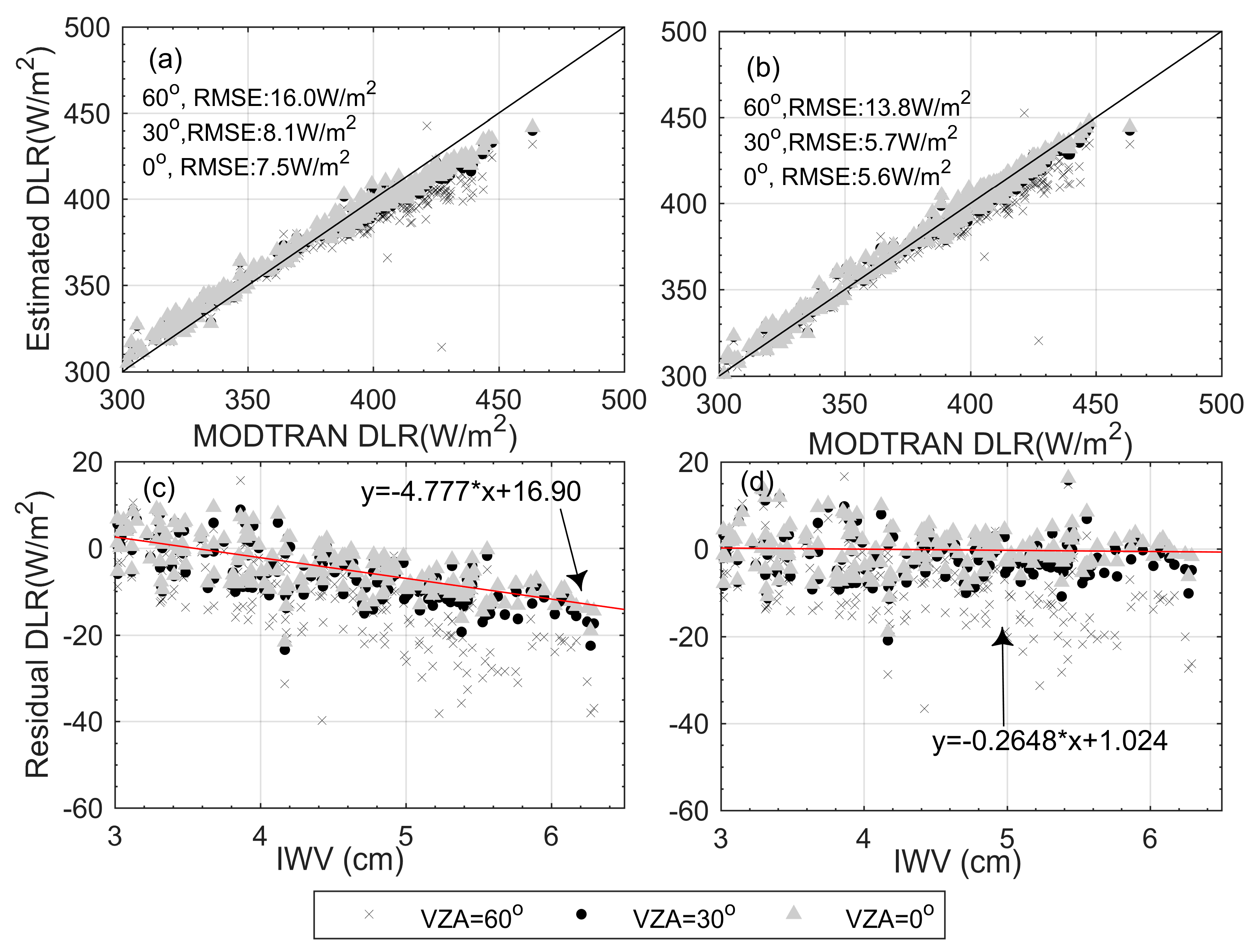
Figure 5.
DLRs calculated from testing dataset using the Yu2013 (a,c) and new parameterizations (b,d), respectively. The algorithms coefficients were deriving from TIGR2002 profiles. Figures (a,b) show the comparison between the estimated and the MODTRAN-simulated DLRs. Figures (c,d) show the residuals of the predicted DLR, which vary with water vapor content for different VZAs, assuming δTs,a = 0 K.
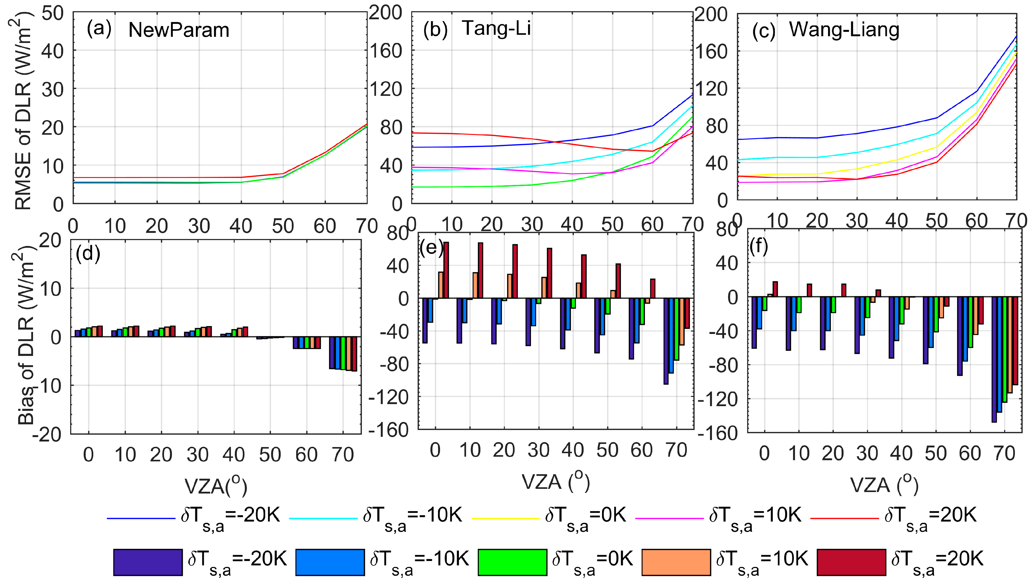
Figure 6.
Figures (a–f) illustrate the RMSE and Mean-Bias-Error (MBE) between the actual and estimated DLRs versus VZA and δTs,a for conifer surface and for NewParam (a,d), Tang-Li algorithm (b,e), and Wang-Liang algorithm (c,f), respectively.
Figure 6.
Figures (a–f) illustrate the RMSE and Mean-Bias-Error (MBE) between the actual and estimated DLRs versus VZA and δTs,a for conifer surface and for NewParam (a,d), Tang-Li algorithm (b,e), and Wang-Liang algorithm (c,f), respectively.
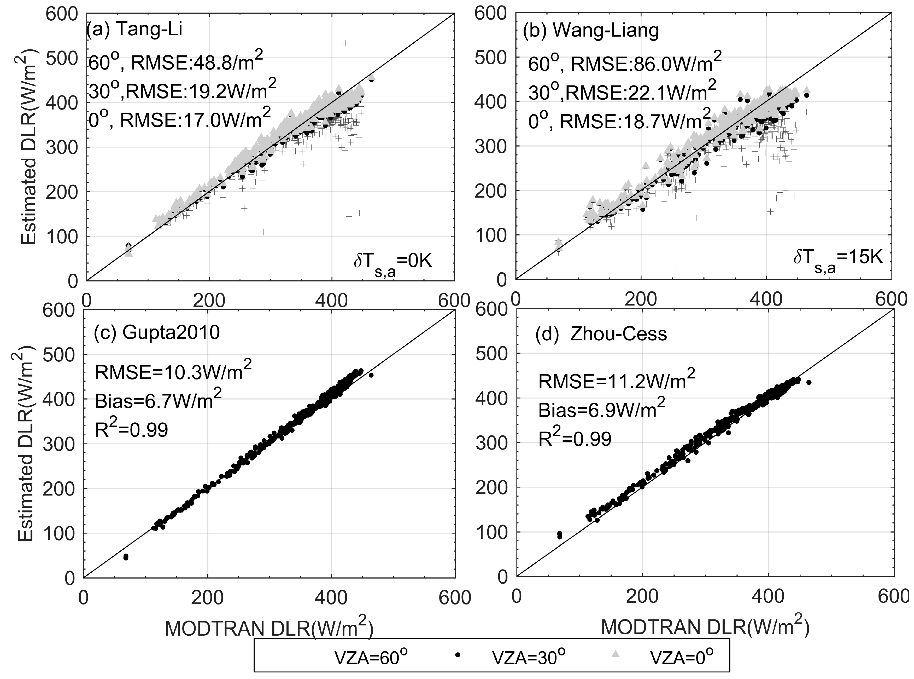
Figure 7.
Comparison of the clear-sky flux calculated from DLR algorithms with those from MODTRAN simulation based on the testing dataset. Figures (a) to (d) represent Tang-Liang, Wang-Li, Gupta2010, and Zhou-Cess algorithms, respectively, and δTs,a is 0 K and 10 K in Figures (a,b).
Figure 7.
Comparison of the clear-sky flux calculated from DLR algorithms with those from MODTRAN simulation based on the testing dataset. Figures (a) to (d) represent Tang-Liang, Wang-Li, Gupta2010, and Zhou-Cess algorithms, respectively, and δTs,a is 0 K and 10 K in Figures (a,b).
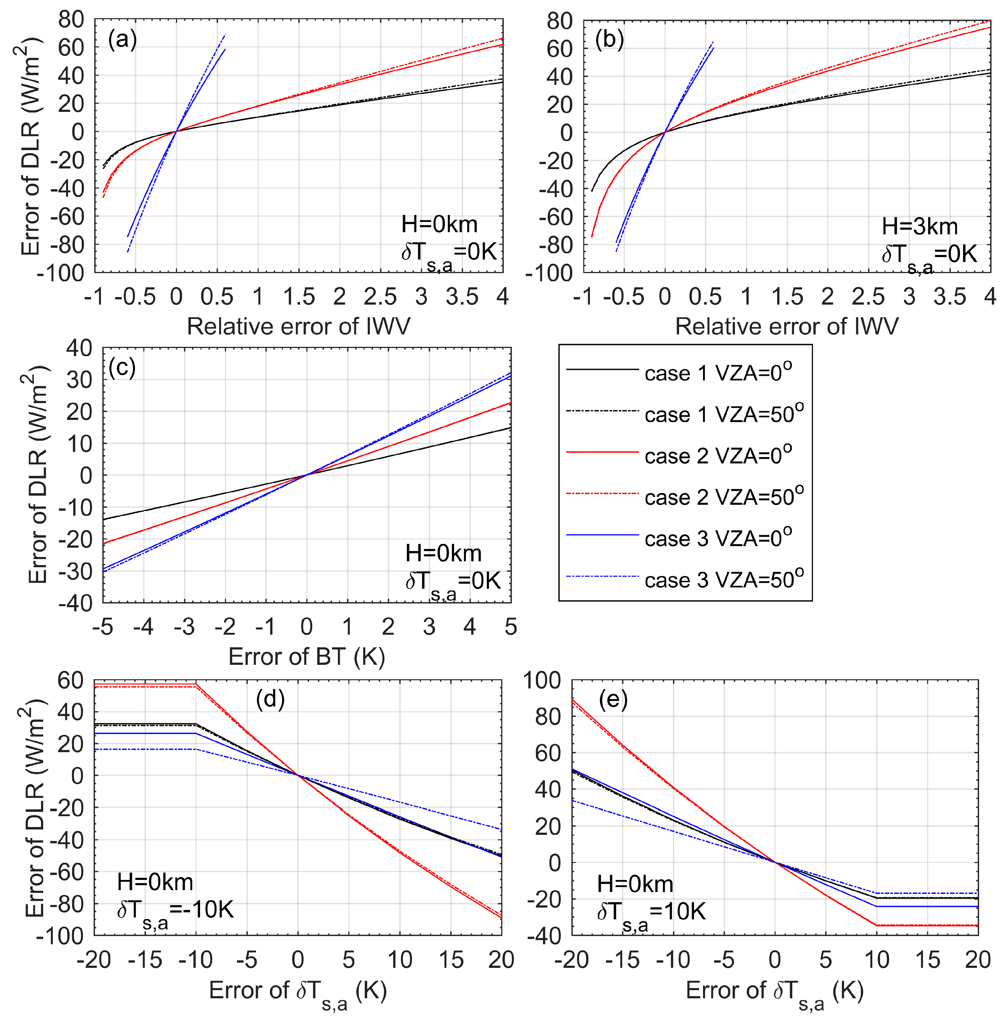
Figure 8.
DLR error versus the error of input parameters such as IWV (a,b), brightness temperature (c), and δTs,a (d,e) under different climate conditions. Cases 1, 2, and 3 represent the conditions of BT = 260 K and IWV = 0.5 cm, BT = 300 K and IWV = 0.5 cm, and BT = 300 K and IWV = 5.0 cm, respectively. Figures (a,b) are for H = 0 and 3.0 km, respectively. Figures (d,e) represent the conditions of δTs,a = −10 and 10 K, respectively.
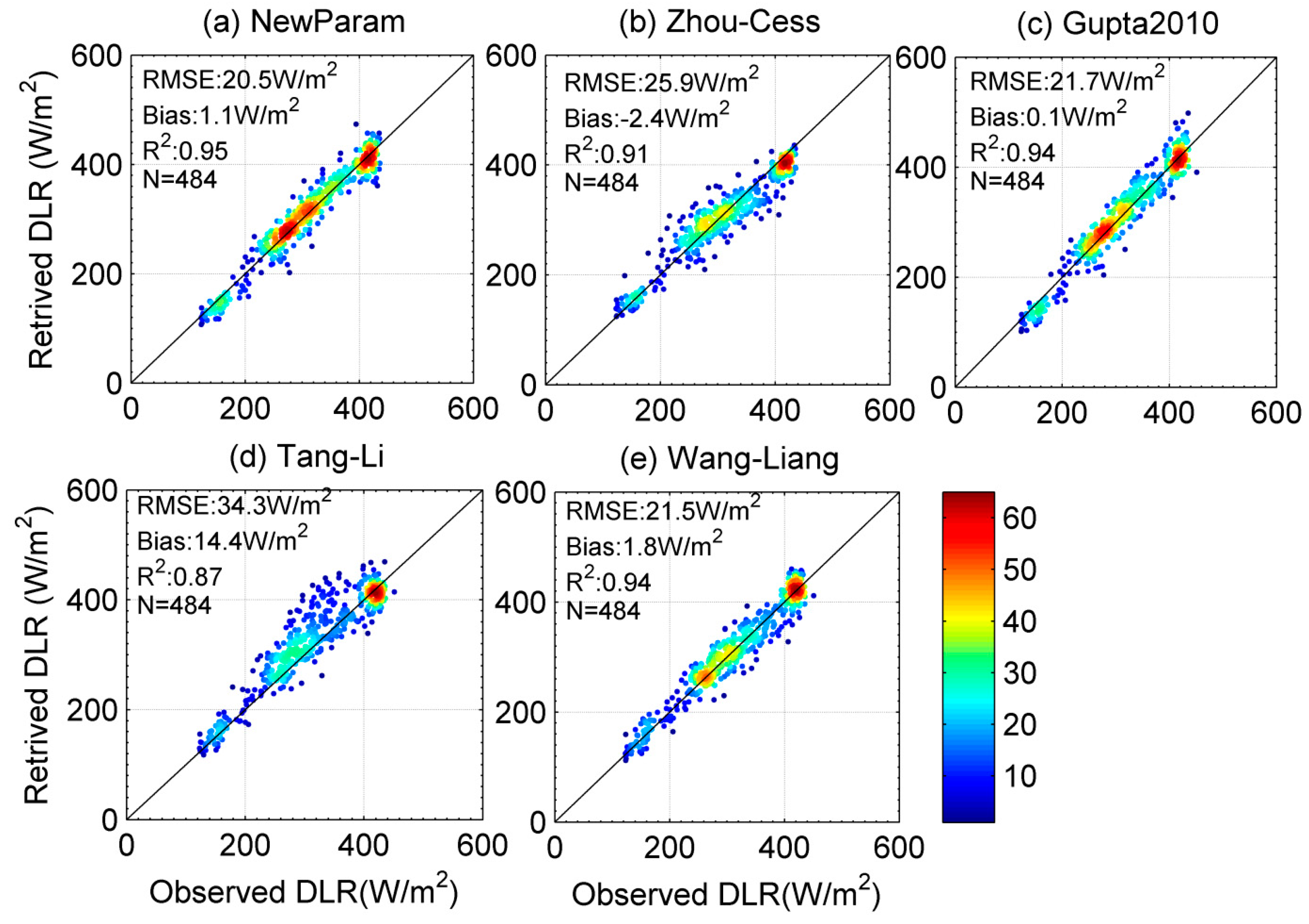
Figure 9.
Comparison between MODIS-estimated DLRs and in-situ measurements at the sites in ordinary regions. Figures (a) to (e) represent the results from the new parameterization (NewParam), Tang-Li, Wang-Liang, Zhou-Cess, and Gupta2010 algorithms. The color bar represents data density that ranges from 0 to 100 percent of the data.
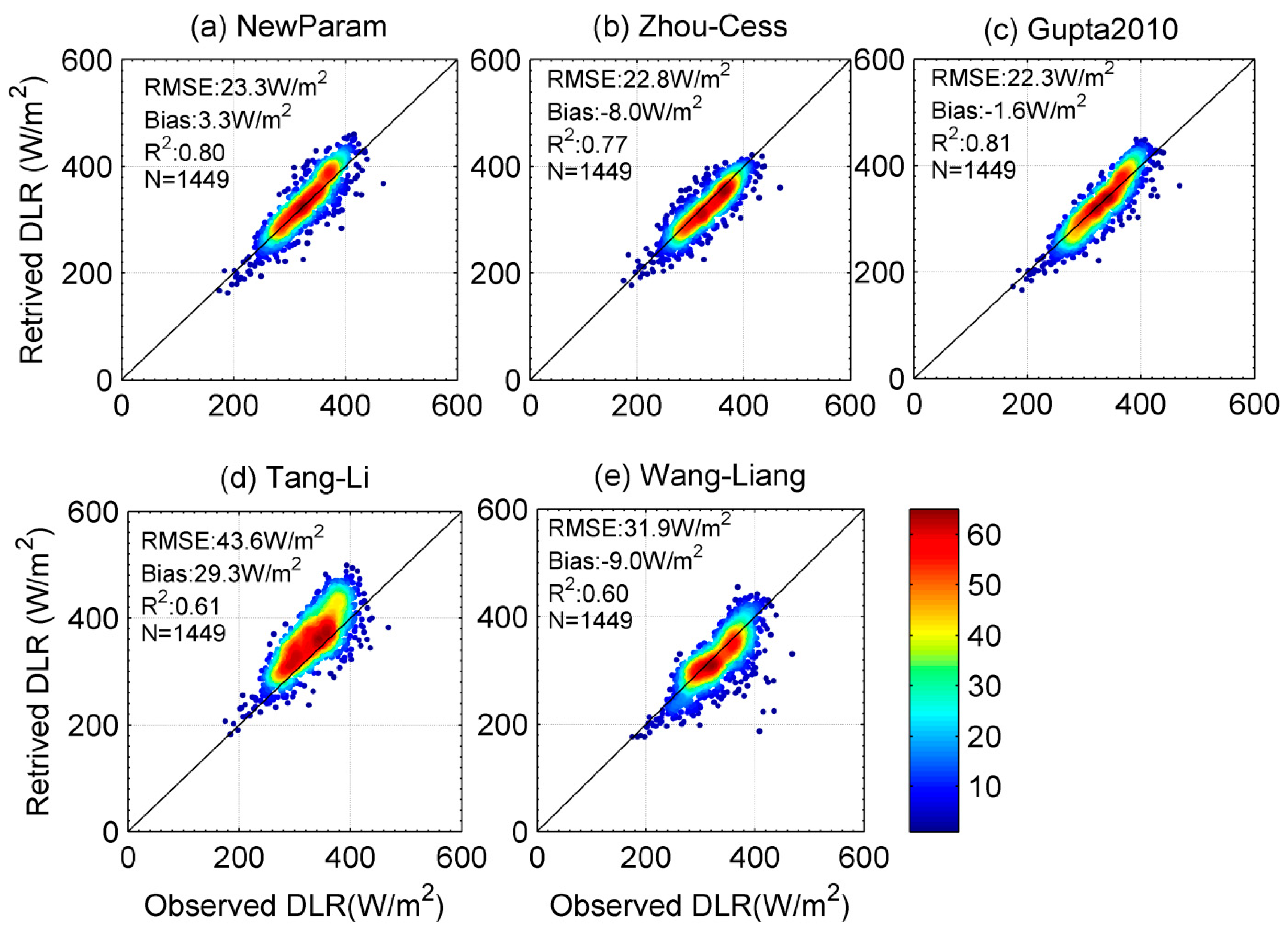
Figure 10.
Same as
Figure 9 but for the sites in the arid regions. Figures (
a) to (
e) represent the results from NewParam, Tang-Li, Wang-Liang, Zhou-Cess, and Gupta2010 algorithms.
Figure 10.
Same as
Figure 9 but for the sites in the arid regions. Figures (
a) to (
e) represent the results from NewParam, Tang-Li, Wang-Liang, Zhou-Cess, and Gupta2010 algorithms.
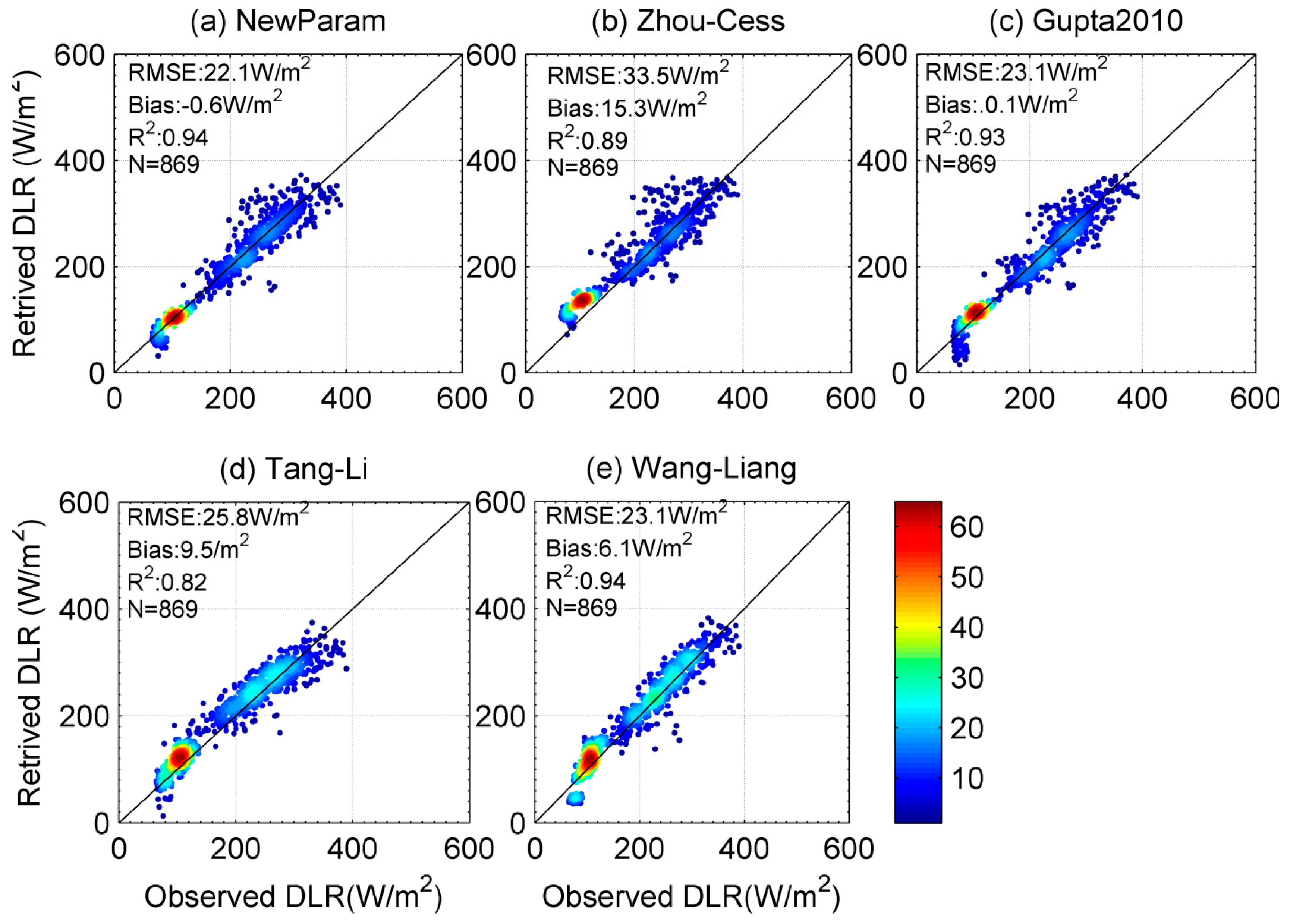
Figure 11.
Same as
Figure 9 but for the sites in the high-altitude regions. Figures (
a) to (
e) represent the results from NewParam, Tang-Li, Wang-Liang, Zhou-Cess, and Gupta2010 algorithms.
Figure 11.
Same as
Figure 9 but for the sites in the high-altitude regions. Figures (
a) to (
e) represent the results from NewParam, Tang-Li, Wang-Liang, Zhou-Cess, and Gupta2010 algorithms.
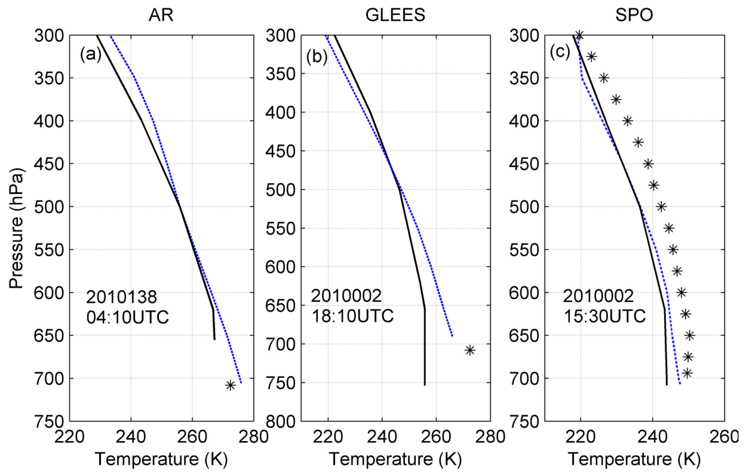
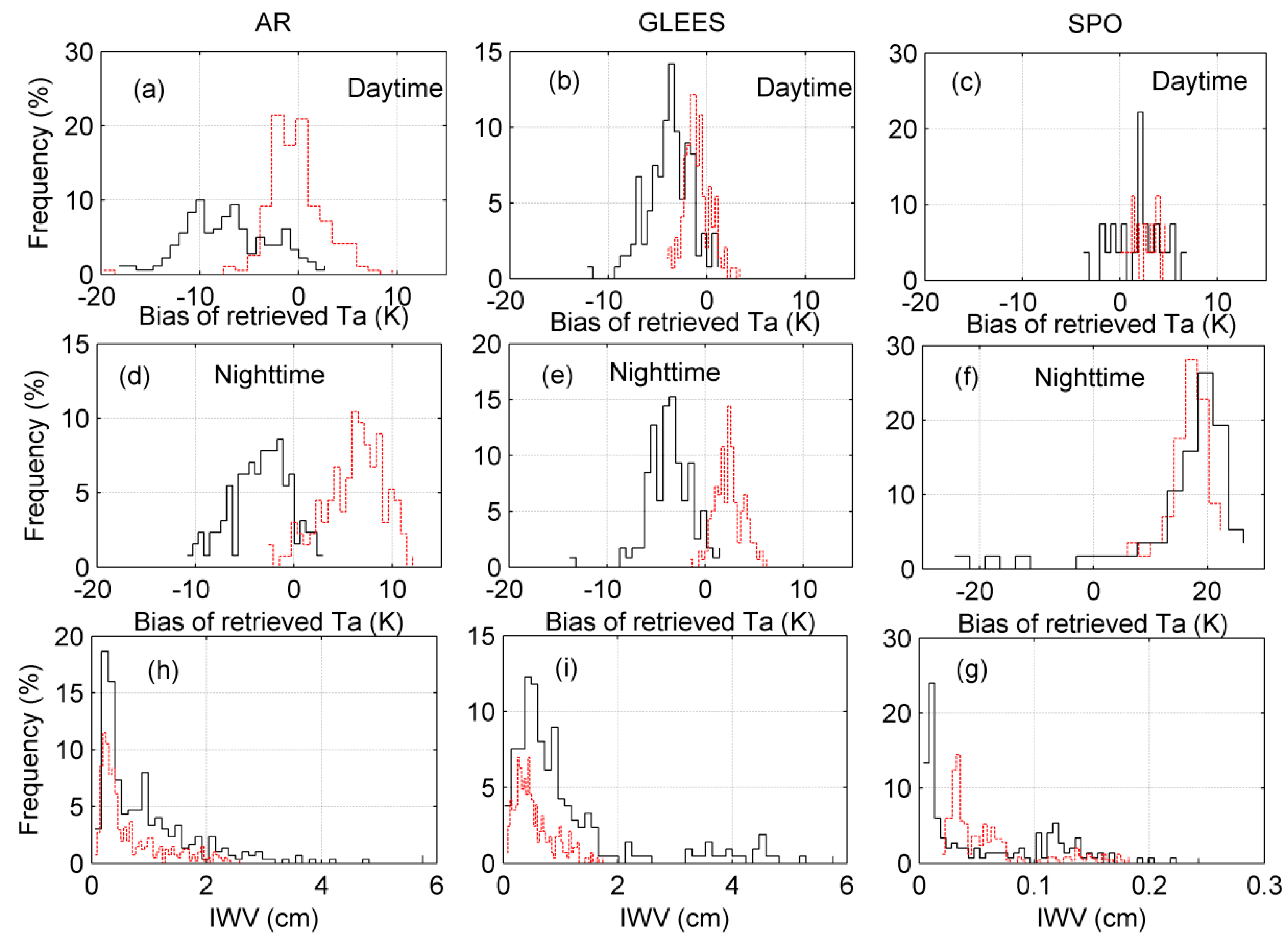
Figure 12.
Vertical distribution of air temperatures from the National Centers for Environmental Prediction (NCEP) and MOD07 profiles at sites Arou (AR), US-GLE Wyoming (GLEES), and South Pole (SPO). The solid line, dashed line, and asterisk represent MODIS, NCEP, and field-measured data, respectively.
Figure 13.
Comparison of MODIS-derived atmospheric parameters with those from NCEP at the sites AR (left column), GLEES (middle column), and SPO (right column). The solid line and dashed line represent parameters from MODIS and NCEP, respectively.
Figure 13.
Comparison of MODIS-derived atmospheric parameters with those from NCEP at the sites AR (left column), GLEES (middle column), and SPO (right column). The solid line and dashed line represent parameters from MODIS and NCEP, respectively.
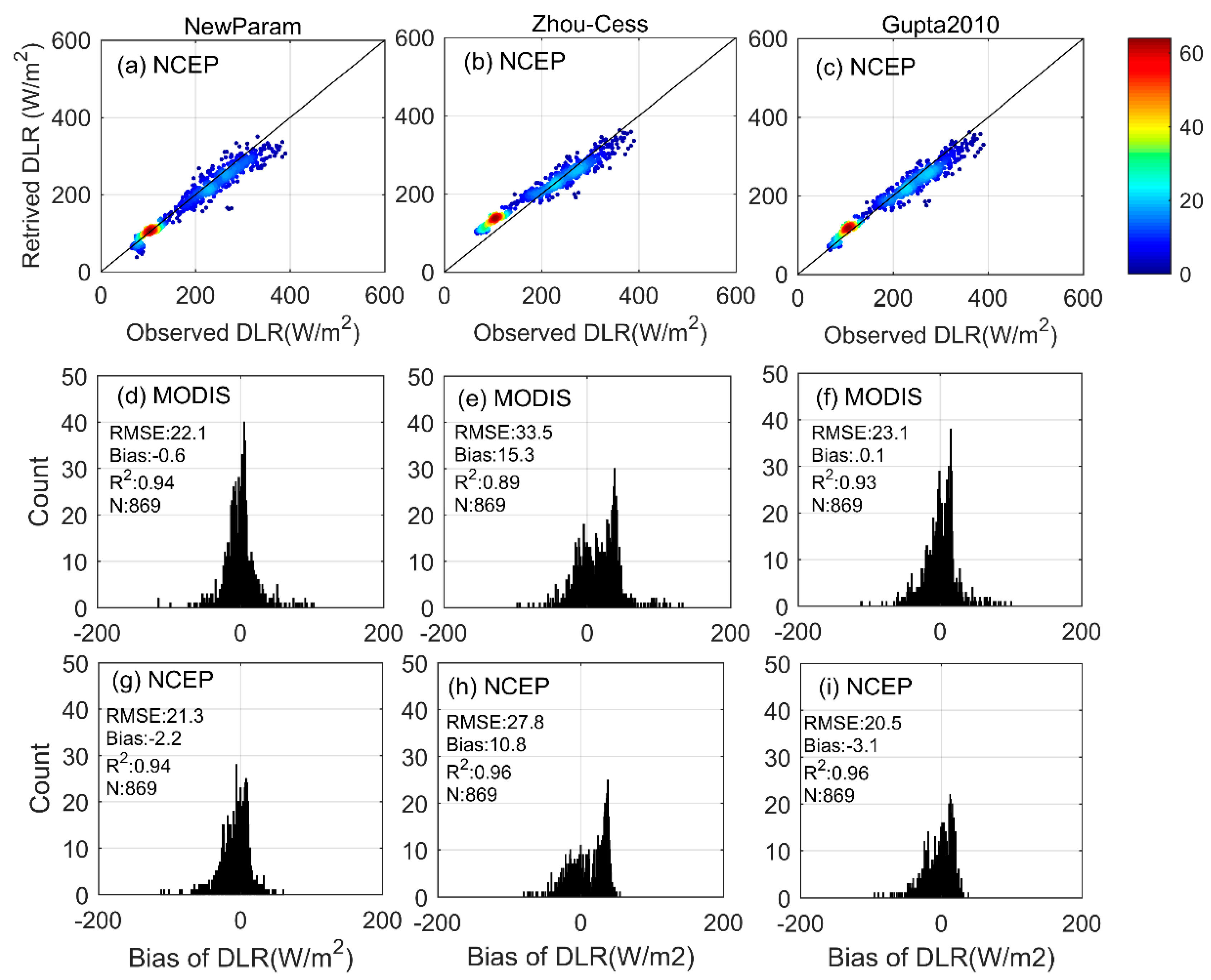
Figure 14.
The results of DLRs at the sites in high-altitude regions. Scatter plot between DLRs estimated from NCEP atmospheric parameters and observed DLR are shown in (a–c). Error histograms between observed and retrieved DLRs from MODIS (d–f) and from NCEP (g–i). Bias was computed as retrieved minus observed values. The left, middle, and right panels represent the results from the new parameterization, the Zhou-Cess, and the Gupta2010 algorithms, respectively.
Table 1.
Clear-sky downward longwave radiation (DLR) algorithms.
Table 1.
Clear-sky downward longwave radiation (DLR) algorithms.
| Authors | Abbreviation | Algorithm 1 |
|---|
| Zhou et al. [25] | Zhou-Cess | |
| Gupta et al. [22] | Gupta2010 | |
| Tang and Li [30] | Tang-Li | , |
| Wang and Liang [31] | Wang-Liang | |
| Yu et al. [36] | Yu2013 | |
Table 2.
Error distribution statistics for IWV greater than 3.0 cm and δTs,a = 0 K.
Table 2.
Error distribution statistics for IWV greater than 3.0 cm and δTs,a = 0 K.
| Sensor Zenith View Angle | Range of Error (W/m2) | Yu2013 | NewParam |
|---|
| VZA = 0° | [−20, 15] | 99.5% | 100% |
| [−40, −20] | 0.5% | 0% |
| VZA = 30° | [−20, 15] | 98.9% | 99.5% |
| [−40, −20] | 1.1% | 0.5% |
| VZA = 60° | [−20, 15] | 73.8% | 90.7% |
| [−40, −20] | 25.1% | 8.2% |
| [−200, −40] | 1.1% | 1.1% |
Table 3.
The mean value of actual and calculated DLRs (DLRact and DLRcal), root mean square error (RMSE), bias, maximum error and minimum error between actual DLRs, and those calculated from training datasets for different surface types when δTs,a = 0 K and VZA = 0° (unit: W/m2).
Table 3.
The mean value of actual and calculated DLRs (DLRact and DLRcal), root mean square error (RMSE), bias, maximum error and minimum error between actual DLRs, and those calculated from training datasets for different surface types when δTs,a = 0 K and VZA = 0° (unit: W/m2).
| Surface Types | Conifer | Soil | Wet Land | Concrete | Dry Grass | Sea Water | Fine Snow | All Types |
|---|
| DLRact | 321.9 | 321.9 | 321.9 | 321.9 | 321.9 | 321.9 | 321.9 | 321.9 |
| DLRcal | 326.7 | 324.9 | 327.6 | 325.5 | 323.8 | 326.8 | 327.1 | 326.1 |
| RMSE | 5.6 | 5.4 | 6.7 | 5.1 | 8.4 | 5.7 | 6.0 | 6.2 |
| Bias | 1.8 | −1.9 | 3.8 | −0.6 | −6.0 | 2.2 | 2.8 | 0.3 |
| Max error | 16.8 | 11.7 | 19.6 | 13.5 | 10.4 | 17.3 | 18.2 | 19.6 |
| Min error | −24.0 | −25.3 | −23.3 | −24.9 | −26.3 | −23.9 | −23.7 | −26.3 |
Table 4.
The definition of each case and the error range of input parameters.
Table 4.
The definition of each case and the error range of input parameters.
| Input Parameter | Value of All Parameters | Error of Input Parameter |
|---|
| IWV | Case 1 (BT = 260 K, IWV = 0.5 cm), δTs,a = 0 K | [−90%, 400%] |
| Case 2 (BT = 300 K, IWV = 0.5 cm), δTs,a = 0 K | [−90%, 400%] |
| Case 3 (BT = 300 K, IWV = 5.0 cm), δTs,a = 0 K | [−60%, 60%] |
| BT | Case 1, Case 2, Case 3, δTs,a = 0 K | [−20 K, 20 K] |
| δTs,a | Case 1, Case 2, Case 3, δTs,a = −10 K | [−5 K, 5 K] |
| Case 1, Case 2, Case 3, δTs,a = 10 K | [−20 K, 20 K] |
Table 5.
Input parameters and data sources used in this study.
Table 5.
Input parameters and data sources used in this study.
| Parameters | Data Source | Algorithms Requiring the Data |
|---|
| Geolocation information and elevation | MOD03, at 1 km | All algorithms |
| Cloud mask | MOD35, at 1 km | All algorithms |
| Viewing zenith angle | MOD03, at 1 km | NewParam, Tang-Li, Wang-Liang |
| TIR channel radiance | MOD021KM, at 1 km | NewParam, Tang-Li, Wang-Liang |
| Water vapor content | MOD05, at 1 km for daytime and 5 km for nighttime | NewParam, Zhou-Cess, Gupta2010 |
| Atmospheric profiles | MOD07, at 5 km | Gupta2010 |
| Air and surface temperatures | MOD07, at 5 km | NewParam, Zhou-Cess, Gupta2010 |
Table 6.
Description of site conditions. Sites used as examples of dry-arid regions are marked with asterisks.
Table 6.
Description of site conditions. Sites used as examples of dry-arid regions are marked with asterisks.
| Site Label | Geographic Name | Latitude/Longitude (°) | Elevation(m) | Period | Surface Type | Instrument | DLR Accuracy | Network |
|---|
| YK | Yingke oasis station, China | 38.850/100.417 | 1519 | 2010 | Cropland | Kipp & Zonen CNR1 | ±10% | WATER |
| AR | Arou freeze/thaw station, China | 38.050/100.450 | 3033 | 2010 | Grass | Eppley PIR | ±5% | WATER |
| HZZ * | Huazhaizi desert station, China | 38.767/100.317 | 1726 | 2010 | Desert | Kipp & Zonen CNR1 | ±10% | WATER |
| SGP-C1 | South Great Plains, Central Facility, America | 36.600/−97.500 | 318 | 2010 | Grass | Eppley PIR | ±2.5% or ±4 W/m2 | ARM |
| NSA-C1 | Barrow, North Slope of Alaska, America | 71.300/−156.600 | 7.6 | 2010 | Tundra | Eppley PIR | ±6 W/m2 | ARM |
| TWP-C1 | Manus Island, Tropical Western Pacific | −2.100/147.400 | 4 | 2010 | Grass | Eppley PIR | ±6 W/m2 | ARM |
| ASP * | Alice Springs, Australia | −23.798/133.888 | 547 | 2010 | Grass | Eppley PIR | ±10 W/m2 | BSRN |
| DOM | Dome C, Antarctica | −75.100/123.383 | 3233 | 2010, [1,2] | Glacier | Kipp & Zonen CG4 | ±3% | BSRN |
| DRA * | Desert Rock, America | 36.626/−116.018 | 1007 | 2010 | Desert | Eppley PIR | ±10 W/m2 | BSRN |
| SBO * | Sede Boqer, Israel | 30.905/34.782 | 500 | 2010 | Desert | Eppley PIR | ±10 W/m2 | BSRN |
| SPO | South Pole, Antarctica | −89.983/−24.799 | 2800 | 2010, [1,7,8] | Glacier | Eppley PIR | ±10 W/m2 | BSRN |
| TAM * | Tamanrasset, Algeria | 22.780/5.510 | 1385 | 2010 | Desert | Eppley PIR | ±10 W/m2 | BSRN |
| FMF | Flagstaff Managed Forest, Arizona | 35.1426/−111.7273 | 2160 | 2010 | Forest | Kipp & Zonen CNR1 | ±10% | Ameriflux |
| GLEES | US-GLE Wyoming, USA | 41.3644/−106.2394 | 3190 | 2010 | Forest | Eppley PIR | ±5% | Ameriflux |
Table 7.
Error statistics for MODIS-derived clear-sky DLR using different algorithms. RMSE, bias, and the square of the correlation coefficients (R2) of all sites and the average values of each type of region are given. RMSE and bias are in units of W/m2. The best results are highlighted in bold, and the worst results are marked with asterisks.
| Site Label | NewParam | Tang-Li | Wang-Liang | Zhou-Cess | Gupta2010 |
|---|
| RMSE | Bias | R2 | RMSE | Bias | R2 | RMSE | Bias | R2 | RMSE | Bias | R2 | RMSE | Bias | R2 |
|---|
| Sites in ordinary regions (DEM < 2000 m) |
| YK | 23.5 | 1.2 | 0.85 | 23.3 | −1.9 | 0.83 | 24.1 | −12.2 | 0.86 | 35.4 * | −21.6 | 0.74 | 21.3 | −9.3 | 0.88 |
| SGP-C1 | 19.4 | 8.0 | 0.91 | 50.2 * | 39.8 | 0.75 | 21.6 | 2.4 | 0.86 | 24.1 | 7.8 | 0.85 | 25.6 | 16.9 | 0.91 |
| NSA-C1 | 17.7 | −1.8 | 0.95 | 24.6 * | 13.3 | 0.93 | 20.3 | 10.1 | 0.94 | 20.6 | 10.4 | 0.94 | 17.7 | −6.3 | 0.95 |
| TWP-C1 | 22.3 * | −9.2 | 0.05 | 19.2 | −8.1 | 0.01 | 19.9 | 6.8 | 0.00 | 20.5 | −16.1 | 0.18 | 19.3 | −11.3 | 0.15 |
| Mean | 20.5 | 1.1 | 0.95 | 34.3 * | 14.4 | 0.87 | 21.5 | 1.8 | 0.94 | 25.9 | −2.4 | 0.91 | 21.7 | 0.1 | 0.94 |
| Sites in dry-arid regions |
| HZZ | 24.3 | −6.5 | 0.90 | 26.7 | 11.8 | 0.84 | 33.2 | −9.0 | 0.82 | 33.2 | −25.1 | 0.84 | 26.3 | −20.5 | 0.91 |
| ASP | 19.5 | 0.6 | 0.82 | 49.9 * | 40.7 | 0.66 | 24.0 | 12.6 | 0.77 | 18.0 | −6.9 | 0.85 | 18.4 | −9.6 | 0.86 |
| DRA | 26.8 | 7.4 | 0.79 | 48.6 * | 35.7 | 0.67 | 30.2 | −21.5 | 0.79 | 23.7 | −2.9 | 0.73 | 21.7 | −1.9 | 0.81 |
| SBO | 23.9 | 0.8 | 0.72 | 48.6 * | 36.4 | 0.59 | 27.7 | −3.3 | 0.63 | 26.1 | −13.4 | 0.66 | 26.1 | −13.8 | 0.71 |
| TAM | 21.9 | 6.7 | 0.77 | 34.4 | 16.9 | 0.46 | 39.2 * | −17.5 | 0.27 | 18.1 | −3.6 | 0.81 | 18.4 | 3.4 | 0.84 |
| Mean | 23.3 | 3.3 | 0.80 | 43.6 * | 29.3 | 0.61 | 31.9 | −9.0 | 0.60 | 22.8 | −8.0 | 0.77 | 22.3 | −1.6 | 0.81 |
| Sites in high-altitude regions (DEM ≥ 2000 m) |
| AR | 23.7 | 9.6 | 0.82 | 23.7 | 8.6 | 0.71 | 21.4 | −4.3 | 0.74 | 27.1 | −10.4 | 0.67 | 27.2 * | −18.8 | 0.83 |
| DOM | 7.8 | 1.4 | 0.56 | 23.3 | 18.0 | 0.31 | 13.4 | 2.9 | 0.30 | 34.8 * | 34.0 | 0.57 | 12.4 | 9.8 | 0.58 |
| SPO | 15.5 | −10.6 | 0.83 | 17.3 | 0.5 | 0.77 | 25.3 | −17.3 | 0.94 | 29.6 * | 27.0 | 0.78 | 24.3 | −12.6 | 0.71 |
| FMF | 22.5 | −8.2 | 0.80 | 26.3 | −0.1 | 0.66 | 19.4 | 5.3 | 0.83 | 23.8 | 3.0 | 0.74 | 17.9 | 5.3 | 0.87 |
| GLEES | 35.7 | 6.3 | 0.62 | 33.3 | 12.6 | 0.65 | 29.4 | 10.9 | 0.72 | 45.4 | 14.2 | 0.39 | 34.6 | 8.7 | 0.61 |
| Mean | 22.1 | −0.6 | 0.94 | 25.8 | 9.5 | 0.92 | 23.1 | 6.1 | 0.94 | 33.5 * | 15.3 | 0.89 | 23.1 | 0.1 | 0.93 |
Table 8.
Same as
Table 7 but for the results in the high-altitude regions. The clear-sky DLRs were estimated using NCEP atmospheric data. The differences between RMSE from NCEP and that from MODIS are displayed in the brackets.
Table 8.
Same as
Table 7 but for the results in the high-altitude regions. The clear-sky DLRs were estimated using NCEP atmospheric data. The differences between RMSE from NCEP and that from MODIS are displayed in the brackets.
| Event Label | NewParam | Zhou-Cess | Gupta2010 |
|---|
| RMSE | Bias | R2 | RMSE | Bias | R2 | RMSE | Bias | R2 |
|---|
| AR | 25.2(1.5) | 7.0 | 0.78 | 21.6(−5.5) | −3.2 | 0.84 | 24.8(−2.4) | −15.6 | 0.87 |
| DOM | 7.8(0) | 3.3 | 0.63 | 35.1(+0.3) | 34.7 | 0.73 | 14.6(+2.2) | 13.3 | 0.74 |
| SPO | 12.4(−3.1) | −8.4 | 0.88 | 29.4(−0.2) | 28.5 | 0.96 | 5.3(−19) | 0.5 | 0.96 |
| FMF | 26.8(4.3) | −3.4 | 0.77 | 20.2(−3.6) | −10.4 | 0.87 | 21.8(+3.9) | −14.5 | 0.88 |
| GLEES | 27.9(−7.8) | −11.4 | 0.74 | 26.3(−19.1) | 2.3 | 0.73 | 27.9(−6.7) | −8.4 | 0.71 |
| Mean | 21.3(−0.8) | −2.2 | 0.94 | 27.8(−5.7) | 10.8 | 0.96 | 20.5(−2.6) | −3.1 | 0.96 |


