Validation of Copernicus Sentinel-2 Cloud Masks Obtained from MAJA, Sen2Cor, and FMask Processors Using Reference Cloud Masks Generated with a Supervised Active Learning Procedure

Abstract

The Sentinel-2 satellite mission, developed by the European Space Agency (ESA) for the Copernicus program of the European Union, provides repetitive multi-spectral observations of all Earth land surfaces at a high resolution. The Level 2A product is a basic product requested by many Sentinel-2 users: it provides surface reflectance after atmospheric correction, with a cloud and cloud shadow mask. The cloud/shadow mask is a key element to enable an automatic processing of Sentinel-2 data, and therefore, its performances must be accurately validated. To validate the Sentinel-2 operational Level 2A cloud mask, a software program named Active Learning Cloud Detection (ALCD) was developed, to produce reference cloud masks. Active learning methods allow reducing the number of necessary training samples by iteratively selecting them where the confidence of the classifier is low in the previous iterations. The ALCD method was designed to minimize human operator time thanks to a manually-supervised active learning method. The trained classifier uses a combination of spectral and multi-temporal information as input features and produces fully-classified images. The ALCD method was validated using visual criteria, consistency checks, and compared to another manually-generated cloud masks, with an overall accuracy above 98%. ALCD was used to create 32 reference cloud masks, on 10 different sites, with different seasons and cloud cover types. These masks were used to validate the cloud and shadow masks produced by three Sentinel-2 Level 2A processors: MAJA, used by the French Space Agency (CNES) to deliver Level 2A products, Sen2Cor, used by the European Space Agency (ESA), and FMask, used by the United States Geological Survey (USGS). The results show that MAJA and FMask perform similarly, with an overall accuracy around 90% (91% for MAJA, 90% for FMask), while Sen2Cor’s overall accuracy is 84%. The reference cloud masks, as well as the ALCD software used to generate them are made available to the Sentinel-2 user community.

1. Introduction

Thanks to their open access policy, their systematic and frequent revisit, and their data quality, the Landsat [1] and Copernicus Sentinel-2 [2] missions have revolutionized the optical Earth observation at a high resolution. Before this open access era, most users only had access to a very limited number of images per year on their sites and used to process the data manually or at least in a very supervised manner. The amount of data provided by these missions pushes the users to automatize their processing, or reciprocally, a manual approach would prevent an efficient use of the data provided by Sentinel-2. To allow a robust and automatic exploitation of Sentinel-2 data, “Analysis Ready Data” (ARD) [3] products are therefore requested by most users. ARD products take care of the common burdens necessary for most applications, which include the cloud detection and atmospheric correction steps.

The detection of clouds and cloud shadows is one of the first issues encountered when processing optical satellite images of land surfaces. The difficulty lies in the large diversity of cloud types and Earth surface landscapes [4]. It is already frequent to confuse bright landscapes with clouds, but moreover, it is especially difficult to detect semi-transparent clouds for which the observed reflectances contain a mixture of cloud and land signals. The detection of cloud shadows is also complex, as a similar low reflectance range can also be frequently observed on targets that are not obscured by clouds. This leads to confusions with water pixels, burnt areas, or topographic shadows. In the case of semi-transparent clouds, shadow detection is even more challenging [5].

Until 2008, when Landsat 8 data started to become free and easily accessible, images with a decametric resolution were expensive, and as a result, users ordered mostly cloud-free images from the image providers. For a given user, the number of images to process was usually low, and the realization of a manual cloud mask was possible. At that time, cloud classification methods existed, but were mainly dedicated to providing a cloud percentage per image in the catalog [6].

The availability of operational imaging satellites, that image all lands frequently, such as Landsat 8 [7] and Sentinel-2 [2], and moreover, the free and open access to these data have prompted new applications based on time series of images covering large territories. For instance, Inglada et al. [8] used all data acquired by Sentinel-2 or Landsat-8 during one year over France, to produce a land cover map of France, applying a supervised classification method. Even if the supervised classification method can cope with the presence of a few outliers in a time series, reliable cloud and shadow masks are important and can only be obtained automatically.

The reliability of the cloud mask is also a key element that determines the noise present in reflectance time series. Figure 1 shows a time series of top of atmosphere reflectances obtained with Sentinel-2 Level 1C data over a mid-altitude meadow in the center of France, for the blue green, red, and near-infra-red spectral bands. The same plot after a good cloud screening (Figure 2, top plot) is much smoother, although several dates were screened because of the cloud cover. It is therefore much easier to process automatically. It may be also noted (Figure 2, bottom plot) that on this site, which usually has a low aerosol content, the effect of atmospheric correction on the smoothness improvement is much less important than the effect of cloud screening.

The Sentinel-2 mission consists of two twin satellites, Sentinel-2A and Sentinel-2B, each one equipped with an optical Multi-Spectral Instrument (MSI). For the next 10 years at least, the Sentinel-2 mission will provide time series of images that combine the following features: thirteen spectral bands from 0.44–2.2 $\mathsf{\mu }$m, high resolution images (10 m–60 m according to the spectral band), and steady and frequent observations. Since the system became fully operational in October 2017, Sentinel-2 has performed acquisitions above each land pixel at least every fifth day.

Several providers have developed so-called Level 2A (L2A) processors, which provide surface reflectances after atmospheric correction and a mask that flags clouds and cloud shadows. At least three organizations are distributing L2A products for Sentinel-2: ESA is distributing L2A data generated with the Sen2Cor processor [9]; the United States Geological Survey (USGS) distributes L2A whose cloud masks come from the FMask algorithm [10]; and the French land data center, named Theia, distributes L2A products generated with the MAJA processor [4]. These methods are explained in the next section.

The Centre National d’Etudes Spatiales (CNES) and the Centre d’Etudes Spatiales de la Biosphère (CESBIO), on the one hand, and the German Aerospace Centre (DLR), on the other hand, separately developed Level-2A processors containing cloud and shadow detection methods applicable to Sentinel-2 time series of images. CNES developed the Multi-sensor Atmospheric Correction and Cloud Screening software (MACCS) ([4,11]), while DLR developed the atmospheric Correction software (ATCOR) ([12]). In 2015, the institutes decided to merge their efforts to develop the MACCS-ATCOR Joint Algorithm (MAJA). MAJA is built on the structure of MACCS, whose methods are extended with a few complementary elements from ATCOR.

Sen2Cor and FMask are mono-temporal methods that use only the image to process and determine the cloud cover, while MAJA methods exploit multi-temporal information. Although some cloud detection methods based on machine learning algorithms are starting to appear ([13,14]), the three methods we selected are rule-based methods that apply thresholds to selected features.

In order to compare the results provided by the three processors quantitatively, reference cloud masks are necessary. To our knowledge, there is no in situ reference database that provides the cloud cover on a regular basis, with a good coverage at a decametric resolution. The validation of cloud masks classically relies on manually-classified images ([13,15]) or polygons selected in a large number of images ([16,17]). Such a validation dataset has already been generated for Sentinel-2 ([16]). A human operator selected and labeled polygons within a set of images, but looking at the selected polygons, we found that the authors had avoided selecting pixels near the cloud limits, where part of the difficulty and subjectivity of identification lies. For a more complete validation, we needed reference cloud masks for which all the pixels would be classified. To do that with a limited amount of manual work, we developed a new method based on machine learning.

As for most existing methods, the generation of our reference masks relies on the ability of well-trained human operators to recognize a cloud, a shadow, or a cloud-free pixel. However, since it would take too long for an operator to classify manually all the pixels of an image, we decided to use an active machine learning algorithm. Our method, named Active Learning Cloud Detection (ALCD), is iterative. The operator labels a small number of pixels, which are used to train a machine learning algorithm, which is used to produce a classification. After this step, the operator visually determines the possible imperfections of the classification and labels new pixels where the classification is wrong or uncertain. This procedure is iterated several times to get a satisfying reference cloud mask.

The article is organized as follows: Section describes the dataset used in the study. Section 3 recalls the detection methods used for Sen2Cor, FMask, and MAJA. Section 4 describes the ALCD method and its validation, and Section 5 describes and discusses the comparison of the validation results of the three selected operational processors.

2. Validation Results for Operational Processors and Discussion

We selected 10 sites and 32 Sentinel-2 L1C scenes, described in

Table 1. Description of each scene used as reference.

Location	Tile	Date	Scene Content
Alta Floresta(Brazil)	21LWK	05 May 2018	Scattered small cumulus
Alta Floresta (Brazil)	21LWK	09 June 2018	Thin cirrus
Alta Floresta (Brazil)	21LWK	14 July 2018	Mid=altitude small clouds
Alta Floresta (Brazil)	21LWK	14 August 2018	Thin cirrus
Arles (France)	31TFJ	17 September 2017	Large cloud cover
Arles (France)	31TFJ	02 October 2017	Thick and thin clouds
Arles (France)	31TFJ	21 December 2017	Mid-altitude thick clouds and snow
Gobabeb (Namibia)	33KWP	21 December 2016	Thick clouds above desert
Gobabeb (Namibia)	33KWP	09 September 2017	Small and low clouds
Gobabeb (Namibia)	33KWP	09 February 2018	High and thin clouds
Ispra (Italy)	32TMR	15 August 2017	Clouds over mountains with snow
Ispra (Italy)	32TMR	09 October 2017	Clouds over mountains with snow and bright soil
Ispra (Italy)	32TMR	11 November 2017	Clouds over mountains and mist
Marrakech (Morocco)	29RPQ	17 April 2016	Scattered cumulus and thin cirrus
Marrakech (Morocco)	29RPQ	02 January 2017	Clear image with with snow and two thin cirrus
Marrakech (Morocco)	29RPQ	21 June 2017	Scattered cumulus and some cirrus
Marrakech (Morocco)	29RPQ	18 December 2017	Scattered cumulus and snow
Mongu (Zambia)	34LGJ	12 November 2016	Large thick cloud cover and some cirrus
Mongu (Zambia)	34LGJ	04 April 2017	Clear image and a few mid-altitude clouds
Mongu (Zambia)	34LGJ	13 October 2017	Large thin cirrus cover
Munich (Germany)	32UPU	22 April 2018	Mostly cloud-free with a few small clouds
Munich (Germany)	32UPU	24 April 2018	Large cloud cover with cumulus and cirrus
Orleans (France)	31UDP	16 May 2017	Thick and thin cirrus clouds
Orleans (France)	31UDP	19 Aougust 2017	Large mid-altitude cloud cover
Orleans (France)	31UDP	18 Feburary 2018	Stratus
Pretoria (South Africa)	35JPM	13 March 2017	Diverse cloud types
Pretoria (South Africa)	35JPM	20 August 2017	Scattered small clouds
Pretoria (South Africa)	35JPM	14 October 2017	Large thin cirrus cover
Pretoria (South Africa)	35JPM	13 December 2017	Altostratus and scattered small clouds
Railroad Valley(USA)	11SPC	01 May 2017	Small cumulus over bright soil
Railroad Valley (USA)	11SPC	27 August 2017	Large cumulus over bright soil
Railroad Valley (USA)	11SPC	13 February 2018	Large stratus and some cumulus

which were used to validate the active learning method and then to evaluate the performances of the three selected operational processors. The 10 sites have been chosen in order to ensure a large diversity of the scenes. Several dates at different seasons were selected to obtain various atmospheric conditions, cloud types, and land covers.

Five out of ten sites are mostly covered by vegetation. We chose an equatorial forest site, Alta Floresta in Brazil, two very diverse sites, Arles (France) and Ispra (Italy), ranging from mountains to agricultural plains, and two flatter agricultural sites in Munich (Germany) and Orleans (France), which also include large patches of forests. We also added five arid sites, four in Africa and one in North America, with various degrees of aridity: Gobabeb, Namibia, is a desert site; Marrakech, Morocco, is mainly a high elevation semi-desert, which includes the highest peaks of the Atlas mountains; Railroad Valley (USA) includes very bright patches of sand and some mountains. The two last sites, Pretoria, South Africa, and Mongu, Zambia, contain grassland, savannah, and dry woodland. The sites are also very diverse in terms of elevation, with flat low altitude sites in Orleans, Gobabeb, and Alta Floresta, contrasted sites that go from mountains to sea level (Arles, Ispra), or from 450 m above sea level (a.s.l) to above 4000 m for Marrakech, and flat more elevated sites in Munich (600 m a.s.l), Mongu (800 m a.s.l), Railroad valley (1200 m a.s.l), Pretoria (1500 m a.s.l).

3. Cloud and Cloud Shadow Detection Methods

The free availability of Landsat time series, which started in 2008 [18], pushed several teams to develop reliable methods to generate cloud masks. The cloud detection methods applied to Landsat rely greatly on the Thermal InfraRed (TIR) bands, using the fact that cloud top temperature is often much lower than the temperature of cloud-free surfaces ([19]). For satellites that lack TIR bands, the classical cloud detection methods consist of a series of rules using thresholds on reflectance or reflectance ratios ([4,10,16,19,20]). They usually combine a set of criteria such as:

• a threshold in the visible range, preferably after a basic atmospheric correction, as surface reflectance is low, while cloud reflectance is higher.
• spectral tests to check that the cloud is white in the visible and near infra-red range.
• a threshold on the reflectance in the 1.38-$\mathsf{\mu }$m band, when it is available (for instance on Landsat-8 and Sentinel-2). This spectral band is centered on a deep water vapor absorption band that absorbs all light in that wavelength passing through the lower layers of the atmosphere ([21]). As a result, only objects on the upper layers can be observed. These objects are usually clouds, but some mountains in a dry atmosphere can also be observed [22].
• thresholds on the Normalized Difference Snow Index (NDSI) to tell snow from clouds, because snow has a much lower reflectance in the short wave infra-red ([23]).

If these criteria are efficient to detect thick clouds and high clouds (when the sensor possesses the 1.38 $\mathsf{\mu }$m band), they usually tend to confuse cloud-free pixels with a high reflectance in the blue, such as bright deserts, and semi-transparent low clouds. Depending on the threshold value, either cloud-free high reflectance pixels will be classified as clouds or thin and low clouds will be classified as cloud-free.

Several arguments also push cloud mask developers to dilate the cloud masks they have obtained.

• Cloud edges are usually fuzzy, and some parts could be undetected.
• Clouds also scatter light to their neighborhood, and this adjacency effect is very complicated to correct as it is very dependent on cloud altitude and thickness, which are not well known.
• Sentinel-2 spectral bands observe the Earth with viewing angles that can differ by about one degree. A parallax of 14km is observed on the ground, which is corrected by the geometric processing of L1C. However, this processing takes only the terrain altitude into account and not of the cloud altitude, resulting in uncorrected parallax errors, which can reach 200m for the bands that have the largest separation (B2 and B8a). Moreover, the acquisition of these two bands is also separated by two seconds, and wind speeds of 10–20 m/s are not uncommon in the atmosphere, adding a few tens of meters to the possible displacement. The parallax effect occurs mostly along the direction of the satellite motion and slightly in the perpendicular direction because of the time difference between acquisitions.

Because of these three items, it is therefore necessary to dilate cloud masks by 200–500 m.

In all this section, we will denote ${\rho }_{band}$ the Top Of Atmosphere reflectance (TOA) for a given spectral band and ${\rho }_{band}^{\ast }$ the TOA reflectance corrected from gaseous absorption and Rayleigh scattering. The interest in performing a basic atmospheric correction before cloud detection is that it allows using the same threshold value whatever the viewing and Sun zenith angles are. Regarding the band names, we used the denomination provided in

Table 2. Spectral bands used in the various cloud detection tests. NIR stands for Near Infra-Red and SWIR for Short Wave Infra-Red.

Band Name	Sentinel-2 Spectral Band	Wavelength (nm)
Blue	B1	445
Green	B3	560
Red	B4	670
NIR	B8a	865
Cirrus	B10	1380
SWIR	B11	1650

.

3.1. MAJA Cloud and Cloud Shadow Detection

For the sake of conciseness, all the details of the method and the threshold values are not provided here, but they have been described in depth in [4]. However, a few changes have recently been made to the method, which are highlighted here.

Sentinel-2’s cirrus band centered at 1.38 $\mathsf{\mu }$m was designed to detect high clouds, as the water vapor in this band absorbs all the light that would otherwise reach the Earth’s surface and travel back to the satellite [21]. Except in very dry atmospheric conditions, the only light reflected to the satellite in this band comes from altitudes above 1000–2000 m. As a result, only clouds or high mountains can be observed in this band. In theory, the threshold to detect clouds with this band should evolve as an exponential function and should depend on the atmospheric water vapor content. In practice, very thin clouds are very frequent, but a large part of them is thin enough to bring very limited disturbance to the surface reflectance in the bands outside the cirrus band. We used for MAJA a quadratic law of variation of the cirrus band threshold with altitude. A high cloud is detected if Equation (1) is verified.

$${\rho }_{cirrus}>0.007+0.007\times h^2$$

(1)

where h is the pixel altitude in km above sea level.

To the classical multi-spectral threshold methods described above, MAJA adds several multi-temporal criteria, because surface reflectances usually tend to change slowly with time. To use multi-temporal criteria, MAJA uses a reference composite image that contains the most recent cloud-free observation for each pixel. At each new image, MAJA updates the composite with the newly-available cloud-free pixels. Due to that, MAJA has to process the data for a given location in chronological order.

The multi-temporal method detects the pixels for which a sharp increase of reflectance in the blue is observed. However, ground surface reflectance can also increase with time, especially if the pixels in the composite have been acquired a long time ago, due to a persistent cloud cover. Because of that, the threshold on blue reflectance increase becomes higher when the time difference between the acquisition and the reference increases. If a pixel is declared cloudy by that criterion, it has to be whiter than in the reference composite image to be accepted as a cloud.

As MAJA is a recurrent method, it needs to be initialized. For that, we have also implemented a mono-temporal cloud mask, which tends to be less selective than the multi-temporal cloud mask. As a result, it is only used when the first image in a time series is processed or when, because of a persistent cloud cover, the most recent cloud-free pixel in the composite is too old to be used to detect clouds (more than 90 days). In [4], a very simple threshold on the blue reflectance was used, but starting from MAJA Version 2.0, we replaced it by the ATCOR mono-temporal cloud mask, defined as:

$$\begin{array}{c}{\rho }_{blue}^{\ast }>0.22 \mathrm{and} {\rho }_{red}^{\ast }>0.15\mathrm{and}\\ {\rho }_{NIR}^{\ast }<{\rho }_{red}^{\ast }\times 2\mathrm{and}\\ {\rho }_{NIR}^{\ast }>{\rho }_{red}^{\ast }\times 0.8\mathrm{and}\\ {\rho }_{NIR}^{\ast }>{\rho }_{SWIR}^{\ast }\end{array}$$

A final control checks the correlation of each cloudy pixel neighborhood with previous images, as already done in [24]. We used a neighborhood of $7\times 7$ pixels, at 240-m resolution. Given that it is very unlikely to observe a cloud at exactly the same place with the same shape in successive images, we discarded all cloud pixels for which a correlation coefficient greater than 0.9 was found.

MAJA tests were not performed at full resolution, but currently at 240 m, in order to (i) spare computation time and (ii) avoid false cloud or shadow detections that could occur at full resolution if spectral bands are not perfectly registered. Moreover, man-made structures, such as buildings, greenhouses, roads, and parking lots can have very diverse spectra and generally contain bright or dark objects that could be classified as clouds or shadows. Of course, due to the processing at a lower resolution, thin clouds with a size of about 100 m can be omitted in the MAJA cloud mask.

Once clouds are detected, it is possible to detect their shadows. The MAJA shadow detection method has been considerably updated since [4] was written, so we describe it here with more details. MAJA also uses a multi-temporal method to detect the darkening of pixels due to cloud shadows. Cloud shadows are usually more noticeable in the infra-red wavelengths, but when vegetation cover changes, the surface reflectances in the NIR and SWIR bands also exhibit more variations with time than for the shorter wavelengths. As a result, the best multi-temporal detection results for cloud shadow were obtained using the red band.

Two cloud shadow masks were generated: a so-called “geometric” one, which only searches for shadows where a detected cloud can cast a shadow, and a “radiometric” one for the shadows that may have been generated by clouds lying outside the image.

The “geometric” shadows algorithm computes the intersection between the zones where there could be a cloud shadow (because of the presence of a cloud in the neighborhood) and the zones in which the darkening in the red band seems high enough. For that, the MAJA cloud mask was used to compute the zone where a cloud shadow could exist, considering cloud altitudes from the ground to ten kilometers. For each altitude, the cloud shadow zone was computed using a geometric projection, accounting for the solar and viewing directions, as in [5].

We then determined a threshold on the relative variation of the reflectance in the red band to detect the real cloud shadows within the possible shadow zone. To do that, we computed a red reflectance ratio:

$$rati{o}_{red}=\frac{{\rho }_{red}^{\ast }\left(D\right)}{{\rho }_{red}^{\ast }\left(D_{ref}\right)}$$

where ${\rho }_{red}\left(D\right)$ is the reflectance of the pixel at date D, and ${\rho }_{red}^{\ast }\left(D_{ref}\right)$ is the reflectance value in the cloud and shadow-free composite reference image (after a basic atmospheric correction, as explained above). A pixel may be a shadow if it belongs to the possible shadow region and if:

$$rati{o}_{red}<T_{shadow}$$

with $T_{shadow}$ a threshold value, which depends on the image content. To compute $T_{shadow}$, a histogram of the red band reflectance ratio was computed for the cloud-free pixels. The threshold value was set to a certain percentage of the cumulative histogram, the actual value depending on the cloud cover proportion (the higher the cloud cover, the higher the percentage). To avoid local over-detections, the area of shadows was tested cloud per cloud to ensure that the cloud shadow area was not greater than the cloud area, with a 20% margin. If it was greater, a lower threshold was used to reduce its size.

For the “radiometric” mask, we used a threshold depending on the actual darkening of the shadows detected in the rest of the image by the previous (“geometric”) algorithm or a default value if no shadow had been detected. As for the cloud detection, a final correlation test was used to eliminate some remaining over-detections.

Finally, as explained in the Introduction, all the cloud and shadows masks were dilated by two coarse pixels, i.e., 480 m.

The MAJA cloud mask is provided as a set of binary bits, which contain the results of each set of cloud masks:

• mono-temporal test
• multi-temporal test
• high cloud
• geometric cloud shadows
• radiometric cloud shadow

and two bits used as a summary of the detection:

• cloud or shadow detected by any of the above tests
• cloud detected by any of the above cloud detection tests

3.2. Sen2Cor Cloud Detection Method

The Sen2Cor cloud detection method is described in depth in ([9]), although this description applies to an older version of Sen2Cor and has not been updated since then. It mainly uses the four classical thresholds defined at the beginning of this section, but in a slightly different manner and with some complementary thresholds.

The specificity of the Sen2Cor method is that each test provides a probability map of cloud presence (between 0 and 1). All these individual probability masks are then multiplied to get a global probability mask. Various thresholds are applied to the global probability mask to get three masks: a low probability cloud mask, recently renamed “unclassified”, a medium probability cloud mask, and a high probability cloud mask.

The global threshold (1) is applied to the red band instead of the blue band. As this test tends to detect too many clouds, several tests on band ratios are passed to avoid detecting clouds on:

• senescent vegetation (using the near infra-red/green ratio),
• soils (using the short wave infra-red/blue ratio),
• bright rocks or sands (using the near-infra-red/sand ratio).

Another test is used to tell snow from clouds, as described in the introduction of this section.

Sen2Cor also detects cloud shadows using the fact that cloud shadows are dark and only keeps the shadows that can be traced back to a cloud. In this study, we had access to Sen2Cor Version 2.5.5.

3.3. FMask Cloud Detection Method

The FMask (Function of mask) method [25] was initially developed for Landsat 5 and 7 and later on extended to Landsat-8 [10]. It involves the surface reflectances and the brightness temperatures of the Thermal Infra-Red (TIR) Channels. In [10] as well, a variant of the method was developed for Sentinel-2 without TIR bands.

The FMask method first computes potential cloud and cloud shadow layers based on single date thresholds including the ones described in the general methods above and, of course, for Landsat only, on the thermal infra-red bands. After this first step, a second pass is used to compute the cloud probability based on statistics computed on the pixels that are not in the potential cloud layer. Pixels with the highest probability are also included in the potential cloud layer. An object-based method segments these layers and tries to match the clouds with their shadows, by iterating on the cloud altitude. If a good match is found, potential shadow objects are confirmed.

In this paper, we had access to the FMask 4.0 version, which is the most recent version of FMask. The improvements brought to the methods of FMask have not been published so far, but they at least include the detection of clouds based on Sentinel-2 observation parallax from [26].

4. Method to Create Reference Cloud Masks

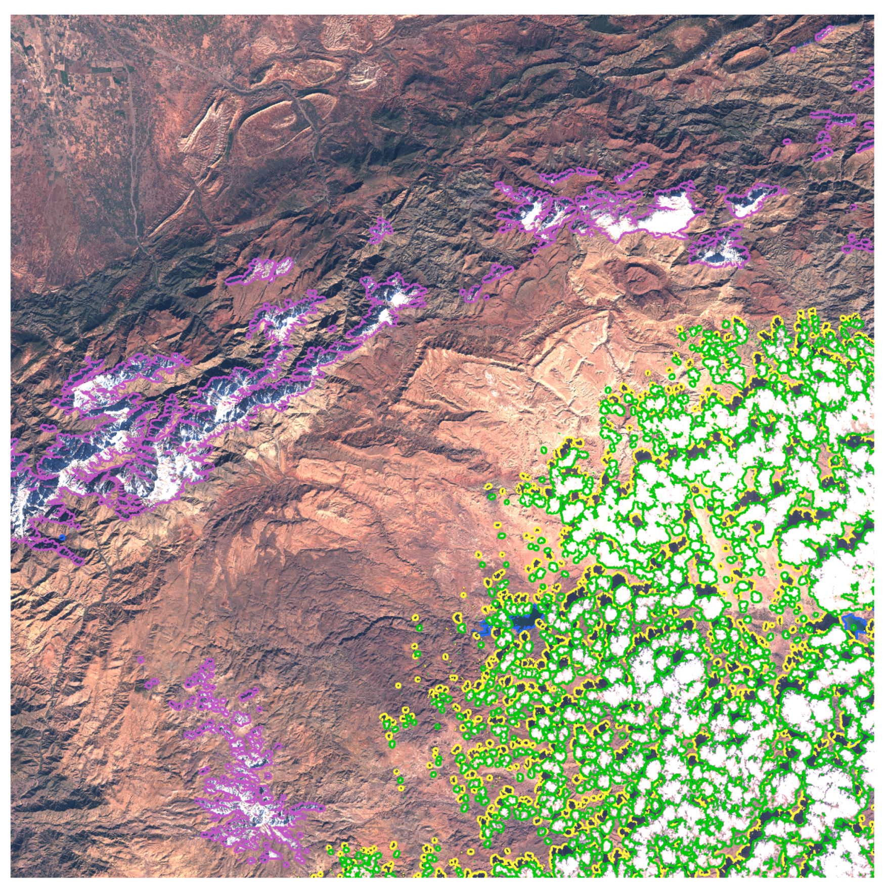
4.1. How to Recognize a Cloud

In Sentinel-2 images, clouds are white and usually have a reflectance higher than that of the underlying surface, especially in the blue band [20]. They also have a greater SWIR reflectance than that of snow [23], and if they are high enough in the atmosphere, they have a non-null reflectance value in Sentinel-2 Channel 10 centered on the band at 1.38 $\mathsf{\mu }$m [21]. They usually also look less sharp than the surface, and their shape changes from date to date in the same location. All these criteria can be used by a human operator to decide which pixels are clouds.

However, the first issue found in trying to build a reference cloud/shadow mask is the lack of an accurate definition of what we should consider as a cloud. As said in [15], “note that a quantitative threshold does not exist to distinguish thin clouds and transparent features such as haze and aerosols, making thin cloud identification inherently subjective to any analyst”. As it is possible, to some extent, to correct reflectances for the effects of aerosols, it is important not to confuse them with clouds. Moreover, even if it is easy to see a thin high cloud on the 1.38-$\mathsf{\mu }$m band, this cloud can still be too thin to have an effect on the surface reflectance of the other channels. As a result, flagging as invalid all the pixels for which the surface reflectance at 1.38 $\mathsf{\mu }$m is not null would result in discarding too much useful information for users.

Finally, the pixels we classified as clouds were either (i) opaque clouds that were easily identifiable, (ii) semi-transparent clouds that were identifiable in the band at 1.38 $\mathsf{\mu }$m, which can be also discerned in the other bands, and (iii) semi-transparent clouds that were identifiable in visible bands, even if not visible in the 1.38-$\mathsf{\mu }$m band. The clouds that were visible in the band at 1.38 $\mathsf{\mu }$m were classified as high clouds, and the others as clouds.

Snow was distinguished from clouds by viewing the SWIR band at 2.2 $\mathsf{\mu }$m (Band 12) and the digital elevation model. Similarly, shadows are quite easy to distinguish from water thanks to their shapes and textures, and in case of a doubt, we distinguished cloud shadows from other dark features, by checking that there were clouds around that could cast that shadow. It was also possible to tell cloud shadow from topographic shadow using the DEM, and in the case of topographic shadow, the shadow was still visible in another cloud-free image acquired a few days apart. In many cases, thin clouds were observed above cloud shadows, and we classified those as clouds. However, the distinction is not too important as the aim of the cloud shadow detection method is to tell the pixels valid for land surface analysis from the invalid ones.

Finally, water is usually easy to tell from land visually, using the image context, and in the case of mixed pixels, an accurate distinction is not essential, as we considered both pixels as valid for monitoring surface reflectances.

Using these rules, we labeled samples with 6 classes: land, water, snow, high cloud, low cloud, and cloud shadow.

4.2. Active Learning Cloud Detection Method

In order to classify whole images according to the 6 classes defined above, we set up an Active Learning Cloud Detection (ALCD) method. Active learning was introduced in 1994 [27] in the context of text recognition. It was later on introduced in remote sensing [28]. Active learning’s main idea is that the training of a model based on a small ensemble of well-chosen samples can perform as well as a model trained on a large ensemble of randomly-chosen samples. It therefore provides a strategy to reduce the amount of time to devote to the provision of training samples. In classical active learning methods, samples that are automatically selected are proposed to be labeled by the user. We did not fully implement such an active learning method, but, after the first iteration, the user selected samples where the classifier had a low confidence or where it was obviously wrong. We provide here a general description of our methodology, then detail each step more accurately.

• Compute the image features to provide to the classifier.
• While the classification is not satisfactory:
  • Select of a set of samples for the 6 classes. After the first iteration, select these samples where the image classification is wrong or where the classification confidence is low.
  • Train a random forest [29] model with the samples.
  • Perform the classification with the model obtained at Step 2.
• end while.

We chose to generate reference cloud masks at 60-m resolution, which corresponds to the lowest resolution of Sentinel-2 bands.

4.2.1. Feature Selection

In the jargon of machine learning, the features are the information provided to the machine learning method. Regarding image classification, the features are information provided per pixel. In the ALCD method, for each scene, 26 features were computed:

• Twelve bands from the image to classify. Among the 13 available bands, the B8A band was discarded, as its information is redundant with respect to that of B8.
• The Normalized Difference Vegetation Index (NDVI) [30] and the Normalized Difference Water Index (NDWI) [31] of the image to classify.
• The Digital Elevation Model (DEM). Its purpose is two-fold: First, it aims at improving the distinction between snow and clouds, in high altitude areas. Snow is generally present above a given altitude, and the threshold altitude is often more or less uniform on the scene. The combination of information coming from the reflectances and the DEM can help the classifier distinguish between those two classes. It can also partially avoid the false-positive detection of cirrus with Band 10 (1.38 $\mathsf{\mu }$m) over mountains.
• The multi-temporal difference between bands of the image to classify and a clear image. For this, we used a cloud-free date (referred to as the “clear date”) acquired less than a month apart from the date we wanted to classify. We provided the difference of these images to the classifier, for all bands except Band 10, as it does not allow observing the surface except at a high altitude. Band 8A was also discarded, for the reason exposed above. Thus, 11 multi-temporal features were computed, from all the other bands.
• MAJA also uses a multi-temporal method. In MAJA, the scenes are processed in chronological order using cloud-free pixels acquired before the date to classify. To obtain results that are independent of those of MAJA, the cloud-free reference image used for ALCD was selected after the date to classify. Moreover, the clear date has to be close to the one to be classified, to allow considering that the landscape did not change. Therefore, we constrained the ALCD reference date to be less than 30 days after the date to classify.
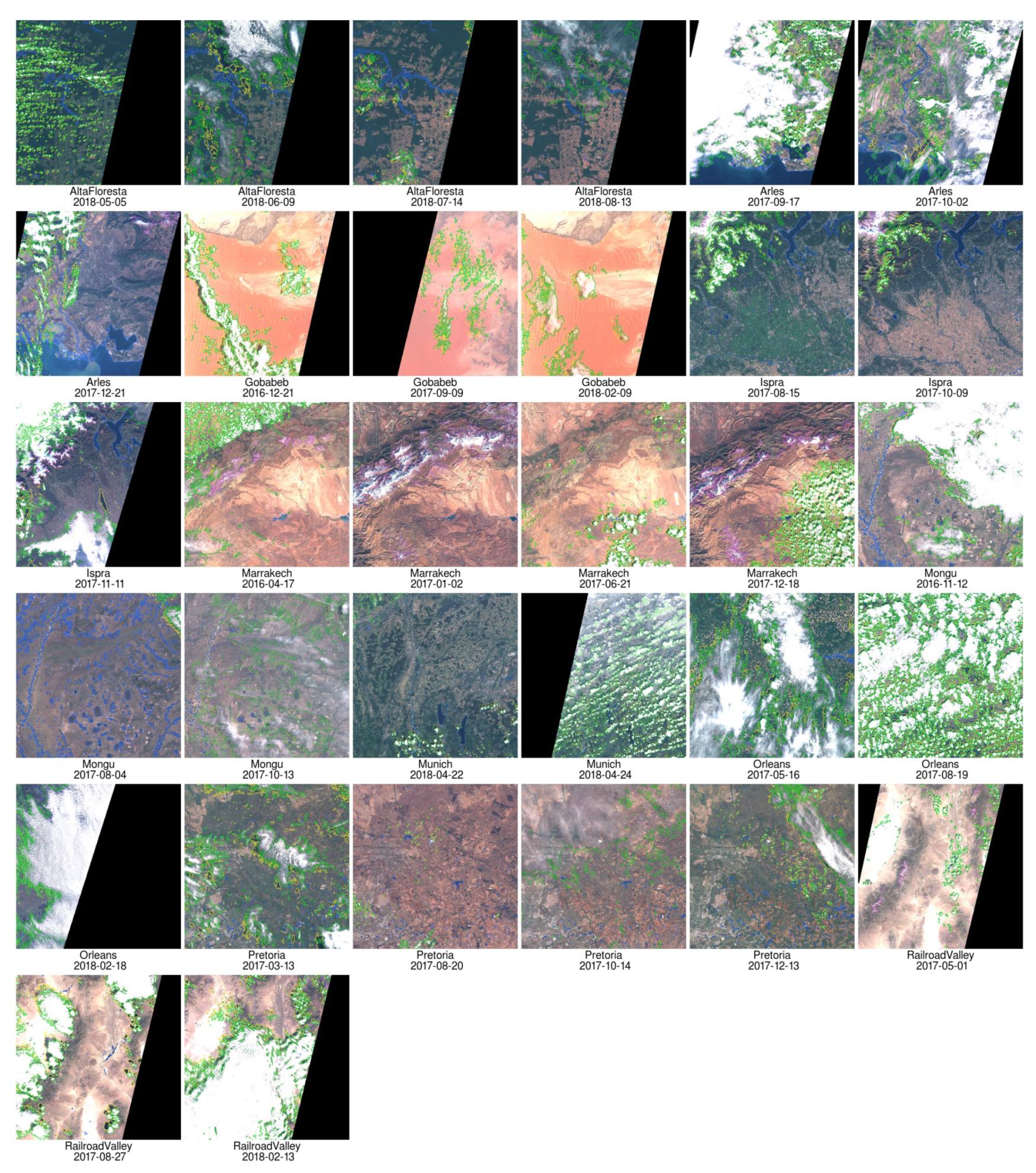
• A side effect of requiring a cloud-free image within a month, but posterior to the date to classify, is that our method cannot produce a reference cloud mask for any Sentinel-2 image. Anyway, there is no need to be exhaustive in the generation of cloud mask validation images. However, the need to find an almost cloud-free image as a reference for the ALCD method prevents us from working on sites that are almost always cloudy, such as regions of Congo or French Guyana for instance. As the multi-temporal features of MAJA would not be very efficient for such regions, this can introduce a small bias in favor of MAJA in our analysis. Still, we included three cloudy sites in our analysis (Alta Floresta, Orleans, Munich) to try to minimize this bias. Finally, the necessity to find a cloud-free reference image has an advantage: it is an objective criterion for the selection of the images to use as reference cloud masks, which avoids a subjective bias for the selection of the images to be processed.

4.2.2. Sample Selection

Along with the features creation, ALCD generates an empty vector data file per class. The user is then invited to populate each file using a GIS software program (we used QGIS [32]). The user can either select the pixels on a “true color” red-green-blue color composite image made with Channels 4-3-2 of Sentinel-2 or on a display of Band 10 to see the potential cirrus clouds. After the first iteration, the user can also view the classification generated at the previous iteration, as well as a confidence map described in the next paragraphs. This information is used to select and label samples where the classification looks wrong or where the confidence is low.

Before producing a large quantity of cloud masks, we studied whether it was more efficient to label points or polygons. By efficient, we mean the possibility to obtain a reliable classification quickly. Polygons have been used by [16] and other authors [33]. The main advantage of a polygon is that it allows selecting a large number of pixels. Therefore, for a similar number of clicks, the number of training samples will be greater with polygons than with points. However, it is time consuming to draw polygons while making sure that they do not include any other class, and it is highly likely that the pixels belonging to a given polygon carry similar information that does not improve the description of the class.

On the contrary, points can be placed quickly in a precise manner, even close to the border of clouds or on small areas. Finally, the diversity of pixels is far greater in the case of points rather than polygons. We thus decided to use points, after several tests on real cases.

The reference samples have been selected according to the principles exposed in Section 4.1. We also paid attention to selecting a number of samples proportional to the area represented by each class, with some increase for classes covering a small area, such as shadow or water. On the 32 scenes we classified, a mean of 120 samples was selected for the first iteration and about 300 points on average. To increase the information provided to the classifier, a data augmentation was done, which consisted of adding pixels in the 3 by 3 pixel neighborhood of 60-m pixels.

4.2.3. Machine Learning

For the machine learning part, we used the Orfeo Tool Box (OTB) [34], which is an up-to-date satellite image processing library distributed as open source software. After several tests, we found that the Random Forest (RF) classifier [29], provided the best results with a shorter training time, as [35] assessed.

4.2.4. Classification and Confidence Evaluation

At each iteration, after having trained a model, the classifier produces a classification map and a confidence map. The random forest classification method produces a large number of binary decision trees, which are used as a committee of classifiers. A vote is then performed, and the class that receives a majority of votes is chosen for each pixel. OTB also returns a confidence map, which is, for the random forest classifier, the proportion of votes for the majority class [34]. For each pixel, a confidence score between 0 and 1 is therefore given.

The confidence map can be used to help the operator select the next samples to classify. A map of low confidence regions is provided to the operator by applying a median filter to the confidence map to reduce its complexity. A layer style with discrete colors is provided to the users, to improve the readability of the map with QGIS.

With those two maps, the user can choose where it is interesting to add new labeled samples. He/she usually has to iterate a couple of times before reaching a satisfying result. When the user is satisfied with the maps, he/she can stop the iterative process and decide to use the last classification as the final one.

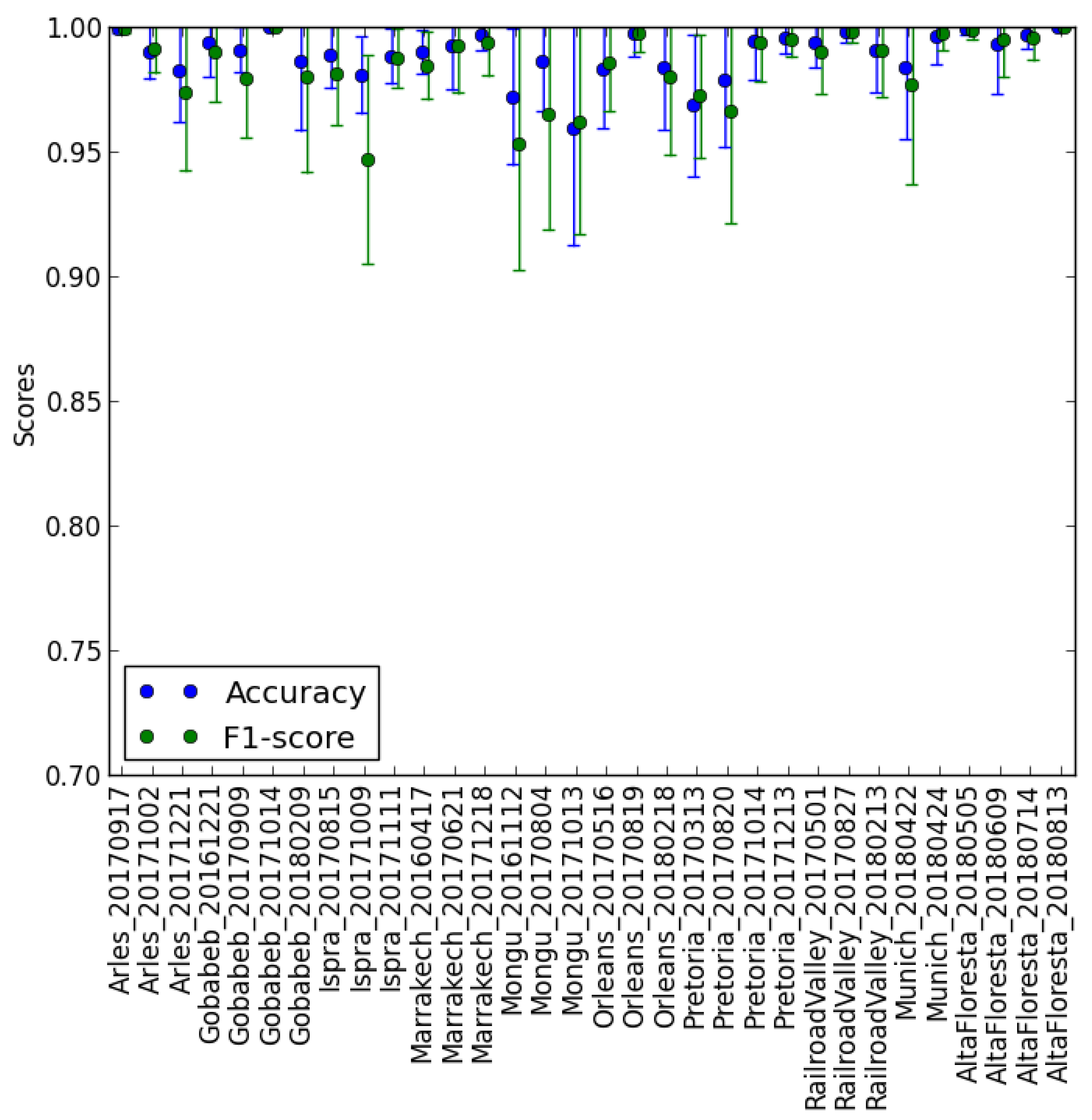
4.3. Validation of ALCD Masks

4.3.1. Visual Evaluation

The simplest option is to check visually if the masks are consistent with the corresponding image. This is done by overlaying the contours of the classes on the true color image and comparing the classification map with the original image. An example is available in Figure 3. We checked all our masks this way, and only stopped the iterative process after they were satisfactory. Miniatures of the other scenes are provided in Figure 4 and in the Supplementary Material.

4.3.2. Cross-Validation

A classical way to validate the performances of a classification is to use a part of the available samples for training and another part for validation. However, as the number of samples we had was quite low, using only half of them for the training would probably reduce the performance.

To avoid that, we used, for each scene, a 10-fold cross-validation ([36]), for which the available samples were randomly split into 10 parts. Ten validation experiments were made using each time a different part for validation and the 9 other parts to train the classifier. This enabled us to get an estimate of the quality of the classification and, by analyzing the dispersion of results for the 10 validation experiments, to check the stability of the result.

As our end goal was to provide accurate binary validity masks, we gathered the low clouds, high clouds, and cloud shadows into the invalid super-class, whereas the land, water, and snow classes were gathered into the valid super-class. Thus, a sample whose real class was low cloud, but which was classified as high cloud was considered correct.

The results were therefore binary. It was therefore possible to compute a number of statistics:

• TP, the number of True Positive pixels, for which both the classified pixel and the reference sample were invalid,
• TN, the number of True Negative pixels, for which both the classified pixel and the reference sample were valid,
• FN, the number of False Negative pixels, for which the classified pixel was valid and the reference sample was invalid,
• FP, the number of False Positive pixels, for which the classified pixel was invalid and the reference sample was valid

From these quantities, we can compute the overall accuracy, which is computed as $\frac{\mathrm{TP}+\mathrm{TN}}{\mathrm{TP}+\mathrm{TN}+\mathrm{FP}+\mathrm{FN}}$; it is the quantity we tried to maximize.

We can also compute the recall (or sensitivity or user’s accuracy) as $\frac{\mathrm{TP}}{\mathrm{TP}+\mathrm{FN}}$ and the precision (or producer’s accuracy) as $\frac{\mathrm{TP}}{\mathrm{TP}+\mathrm{FP}}$. The recall is the proportion of true positives that have been detected. A recall of 100% means all the true positive pixels (clouds or shadows) have been detected, while a precision of 100% means that no valid pixel was classified as invalid. The F1-score is defined as the harmonic mean of recall and precision, which can also be written as: $\frac{2\mathrm{TP}}{2\mathrm{TP}+\mathrm{FP}+\mathrm{FN}}$.

The resulting metrics for all the 32 scenes are plotted in Figure 5. The global mean accuracy was 98.9%, the mean F1-score 98.5%, the precision 99.1%, and the recall 97.8%. All these figures indicate a good overall quality of the classifications.

The maximum standard deviation of the overall accuracy was 4%. One should note that, after the first iteration, the active learning procedure led us to label samples where the classification was not easy. Consequently, the accuracy and F1-score of the 10-fold cross-validation were computed with mainly difficult cases, which probably provided an underestimate of the classification’s real performance.

4.3.3. Comparison with an Existing Dataset

Hollstein et al. created a publicly-available database [16]. It consists of manually-classified Sentinel-2A images with polygons. Their classes were the same as the ALCD ones: cloud, cirrus, snow/ice, shadow, water, and clear sky. A direct comparison is therefore possible. As only one of the images they classified was part of our 32 scenes, we decided to classify 6 additional scenes with ALCD that are part of their dataset. We selected images for which a clear image was available within a month of the desired date. This dataset was not used as the reference image for the validation of operational cloud masks in Section 5, because a large part of the images were acquired very early in Sentinel-2’s life when the acquisitions of Sentinel-2 were not steady yet and some auxiliary files were sometimes incorrect.

The comparison of masks showed a very good agreement, but we noticed on one image that the “shadow” class from the Hollstein dataset also included terrain shadows. On another image, a few polygons with the “cirrus” class were not thick enough to be classified as clouds according to our criteria defined above. Therefore, on those two images, along with the unchanged original reference cloud masks from Hollstein et al., a corrected version of the dataset was produced, to validate the ALCD output more accurately. The results of the correctly-classified pixels are given in

Table 3. Comparison of ALCD masks to Hollstein reference masks on 7 scenes. The mean is weighted by the number of pixels in the polygons.

Tile	Date	Clear Date	Nb. of Pixels in the Polygons	% of Correctly Classified Pixels
				with the Original Dataset	with the Modified Dataset
29RPQ	17 Nov. 2016	27 Apr. 2016	19,371	99.8%	99.8%
32TMR	23 Mar. 2016	26 Mar. 2016	11,558	99.9%	99.9%
32TNR	08 Nov. 2016	29 Oct. 2016	8547	99.2%	99.2%
33UUU	17 Aug. 2016	27 Aug. 2016	3372	98.0%	98.0%
35VLJ	31 Aug. 2016	13 Sep. 2016	5996	93.5%	99.7%
37PGQ	06 Dec. 2015	16 Nov. 2015	15,691	96.0%	100.0%
49JGL	26 Jan. 2016	05 Feb. 2016	5961	100.0%	100.0%
Mean				98.3%	99.7%

. It has to be noted that the cloud masks provided by Hollstein et al. do not contain the edges of the clouds where the distinction between valid and invalid pixels is difficult and somewhat subjective. This contributed to the very good agreement between both datasets as some of the most difficult pixels to classify were not included in the analysis. However, still, based on this comparison, we concluded that ALCD can produce satisfactory classifications, consistent with other teams’ work.

4.3.4. Conclusions on ALCD Validation

We used three methods to validate the reference cloud masks provided by the ALCD method. The first one used visual photo-interpretation to check that the obtained results corresponded to our definition of a cloud and a cloud shadow. The second, based on a 10-fold cross-validation, checked that the methodology was able to classify correctly whole images with the information provided by a limited number of manually-labeled samples. The third, which compared ALCD cloud masks with other cloud masks from Hollstein et al. [16], showed that our definition of clouds was consistent by 98.3% with that of other experts.

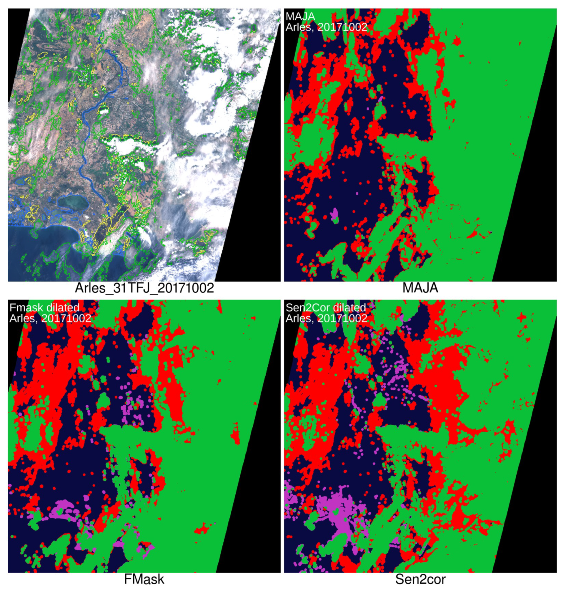
5. Validation Results for Operational Processors and Discussion

As mentioned above, in this study, we compared the performances of three operational cloud mask processors (MAJA Version 3.2, Sen2Cor Version 2.5.5, and FMask Version 4.0), over the 32 scenes described in Section 2. For each processor, we selected the most recent version we had access to, even if this version was not currently used in the operational ground segments. This choice was made to obtain a consistent level of progress among these codes and because we can expect that the ground segments will be updated soon to use these newer versions. As a result, the performances obtained were probably better than those obtained in the official products delivered before our work. Each of the three processors used a particular set of classes for its mask output. There is for instance no cirrus class for FMask, or the absence of distinction between a medium probability cloud and a high probability cloud in MAJA and FMask, which is present in Sen2Cor. In order to compare the results fairly, the multi-class classifications were transformed into binary classification: each pixel was thus classified as valid or invalid, which is moreover what most users need to know: Is a pixel valid to monitor surface reflectance or not ?

For MAJA, a pixel is valid if its cloud/shadow mask value is zero, and invalid otherwise. The invalid pixels included a buffer of 480 m around the detected clouds or shadows.

For Sen2Cor, FMask, and ALCD, the conversion from the multi-class classification to the valid/invalid classes is therefore exposed in

Table 4. Conversion of Sen2Cor mask classes to valid/invalid.

Label	Classification	Binary Classification
0	no data	no data
1	saturated or defective	no data
2	dark area pixels	valid
3	cloud shadows	invalid
4	vegetation	valid
5	bare soils	valid
6	water	valid
7	unclassified	valid
8	cloud medium probability	invalid
9	cloud high probability	invalid
10	thin cirrus	invalid
11	snow	valid

,

Table 5. Conversion of FMask mask classes to valid/invalid.

Label	Classification	Binary Classification
255	null value	no data
0	clear land	valid
1	water	valid
2	cloud shadow	invalid
3	snow	valid
4	cloud	invalid

and

Table 6. Conversion from ALCD classes to valid/invalid.

Label	Classification	Binary Classification
0	null value	no data
2	low clouds	invalid
3	high clouds	invalid
4	cloud shadows	invalid
5	land	valid
6	water	valid
7	snow	valid

.

This conversion allows a direct comparison of the outputs of each chain with the ALCD reference. The workflow for the Sen2Cor processor is given in Figure 6 as an example, and the procedure was the same for MAJA and FMask.

An example of the comparison for the three processors is given in Figure 7, and similar figures for all scenes are provided in the Supplementary Material. On this particular scene, Sen2Cor had a great amount of false valid pixels, i.e., it did not detect clouds where it should have, and FMask also had quite a few false valid pixel, but to a lesser extent. For MAJA, the number of false valid pixels was again lower, but it also had some false invalid pixels, indicating that MAJA detected clouds where there were none. This was partly due to the dilation of clouds used by MAJA.

The differences of approaches concerning dilation are therefore an issue to perform a fair comparison. To solve this issue, we present comparison results expressed in two ways:

• comparison of non-dilated cloud masks, which means we had to erode the MAJA cloud mask, as the dilation was built-in within MAJA;
• comparison of dilated cloud masks, for which we dilated ALCD, FMask, and Sen2Cor using the same kernel as the one used by MAJA; in this comparison, of course, we used the MAJA cloud mask with its built-in dilation.

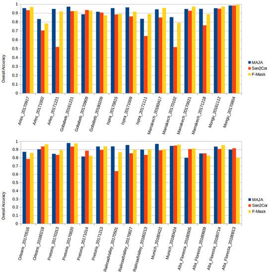
5.1. Comparison of the Results for Non-Dilated Cloud Masks

The results for the 32 scenes are compiled in

Table 7. Accuracy and F1-score for each scene, with the original masks for ALCD, Sen2Cor, and FMask and for MAJA after erosion. In bold, the best metrics for each scene. Dates are written with format YYYYMMDD to save space

Location	Tile	Date	MAJA		Sen2Cor		FMask
			Acc	F1	Acc	F1	Acc	F1
Alta Floresta	21LWK	20180505	0.936	0.444	0.954	0.635	0.954	0.775
Alta Floresta	21LWK	20180609	0.884	0.856	0.855	0.810	0.819	0.760
Alta Floresta	21LWK	20180714	0.971	0.600	0.959	0.152	0.974	0.633
Alta Floresta	21LWK	20180813	0.900	0.849	0.892	0.833	0.788	0.614
Arles	31TFJ	20170917	0.932	0.952	0.866	0.895	0.943	0.959
Arles	31TFJ	20171002	0.864	0.867	0.638	0.546	0.785	0.776
Arles	31TFJ	20171221	0.952	0.802	0.918	0.618	0.951	0.802
Gobabeb	33KWP	20161221	0.952	0.885	0.917	0.736	0.944	0.843
Gobabeb	33KWP	20170909	0.831	0.364	0.980	0.781	0.962	0.606
Gobabeb	33KWP	20180209	0.946	0.710	0.930	0.569	0.919	0.473
Ispra	32TMR	20170815	0.966	0.694	0.973	0.738	0.963	0.730
Ispra	32TMR	20171009	0.979	0.593	0.973	0.438	0.960	0.468
Ispra	32TMR	20171111	0.893	0.824	0.859	0.751	0.917	0.861
Marrakech	29RPQ	20160417	0.925	0.737	0.913	0.621	0.944	0.812
Marrakech	29RPQ	20170102	0.951	0.049	0.908	0.026	0.884	0.018
Marrakech	29RPQ	20170621	0.972	0.786	0.959	0.639	0.979	0.859
Marrakech	29RPQ	20171218	0.937	0.817	0.879	0.518	0.891	0.702
Mongu	34LGJ	20161112	0.969	0.964	0.940	0.927	0.969	0.966
Mongu	34LGJ	20170804	0.995	0.764	0.995	0.769	0.996	0.822
Mongu	34LGJ	20171013	0.857	0.840	0.896	0.892	0.763	0.702
Munich	32UPU	20180422	0.978	0.632	0.982	0.670	0.980	0.695
Munich	32UPU	20180424	0.916	0.944	0.851	0.890	0.888	0.923
Orleans	31UDP	20170516	0.853	0.874	0.710	0.699	0.820	0.838
Orleans	31UDP	20180218	0.938	0.959	0.785	0.841	0.944	0.963
Pretoria	35JPM	20170313	0.922	0.778	0.917	0.753	0.925	0.832
Pretoria	35JPM	20170820	0.995	0.583	0.994	0.504	0.993	0.652
Pretoria	35JPM	20171014	0.828	0.732	0.904	0.866	0.829	0.736
Pretoria	35JPM	20171213	0.964	0.828	0.970	0.857	0.971	0.882
Railroad Valley	11SPC	20170501	0.976	0.549	0.858	0.090	0.905	0.371
Railroad Valley	11SPC	20170827	0.959	0.923	0.894	0.805	0.902	0.841
Railroad Valley	11SPC	20180213	0.899	0.916	0.801	0.820	0.895	0.912

.

Table 7 and Figure 8 show the comparison of the cloud masks provided by the three processors with the reference cloud masks generated with ALCD. The result of one of the masks, the August scene for the Orleans site, is not included, because the cloud cover percentage after dilation was above the 95% threshold, above which MAJA does not issue the product to save computing time and space. In the case of MAJA, the output cloud mask was eroded by 240 m to compensate for the dilation, which is done within MAJA processing. However, the compensation was not perfect, as a dilation followed by an erosion closed the small gaps in the cloud cover.

The results showed quite good overall accuracies, with average values at 93% for MAJA, 91.5% for FMask, and 90% for Sen2Cor. However, in this comparison, the fact that the MAJA cloud mask was dilated then eroded, while the reference and the masks from the two other processors were not, makes a difference, disfavoring MAJA. Moreover, as explained in Section 3, the cloud masks should be dilated.

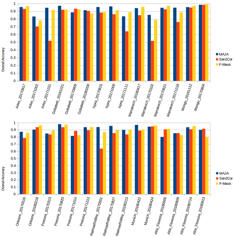
5.2. Comparison of Results for Dilated Cloud Masks

It is therefore more interesting to analyze the results obtained when the cloud masks from the reference and all the processors are dilated. As stated in Section 3.1, MAJA dilates its cloud and shadow masks by 480 m. As a result, the results presented in

Table 8. Accuracy and F1-score for each scene, with the original masks for MAJA and the dilated masks for ALCD, Sen2Cor, and FMask. In bold, the best metrics for each scene. Dates are written with format YYYYMMDD to save space.

Location	Tile	Date	MAJA		Sen2Cor		FMask
			Acc	F1	Acc	F1	Acc	F1
Alta Floresta	21LWK	20180505	0.799	0.615	0.905	0.853	0.913	0.885
Alta Floresta	21LWK	20180609	0.840	0.842	0.854	0.859	0.827	0.831
Alta Floresta	21LWK	20180714	0.936	0.641	0.907	0.409	0.953	0.759
Alta Floresta	21LWK	20180813	0.880	0.845	0.915	0.894	0.801	0.712
Arles	31TFJ	20170917	0.954	0.971	0.931	0.957	0.967	0.979
Arles	31TFJ	20171002	0.830	0.866	0.704	0.759	0.782	0.828
Arles	31TFJ	20171221	0.946	0.867	0.519	0.459	0.918	0.835
Gobabeb	33KWP	20161221	0.971	0.953	0.920	0.856	0.922	0.860
Gobabeb	33KWP	20170909	0.886	0.785	0.934	0.856	0.926	0.828
Gobabeb	33KWP	20180209	0.914	0.733	0.905	0.699	0.873	0.551
Ispra	32TMR	20170815	0.954	0.789	0.884	0.658	0.890	0.659
Ispra	32TMR	20171009	0.962	0.731	0.862	0.489	0.915	0.588
Ispra	32TMR	20171111	0.837	0.814	0.641	0.699	0.889	0.867
Marrakech	29RPQ	20160417	0.941	0.869	0.849	0.724	0.957	0.914
Marrakech	29RPQ	20170102	0.863	0.037	0.517	0.015	0.790	0.020
Marrakech	29RPQ	20170621	0.944	0.769	0.926	0.724	0.971	0.898
Marrakech	29RPQ	20171218	0.947	0.900	0.762	0.634	0.887	0.810
Mongu	34LGJ	20161112	0.954	0.953	0.948	0.947	0.971	0.972
Mongu	34LGJ	20170804	0.984	0.659	0.984	0.708	0.993	0.854
Mongu	34LGJ	20171013	0.782	0.800	0.897	0.916	0.734	0.747
Munich	32UPU	20180422	0.967	0.796	0.890	0.597	0.903	0.627
Munich	32UPU	20180424	0.941	0.967	0.948	0.971	0.960	0.978
Orleans	31UDP	20170516	0.866	0.903	0.785	0.836	0.859	0.898
Orleans	31UDP	20180218	0.902	0.942	0.937	0.965	0.964	0.980
Pretoria	35JPM	20170313	0.845	0.748	0.835	0.768	0.893	0.865
Pretoria	35JPM	20170820	0.979	0.671	0.936	0.483	0.974	0.729
Pretoria	35JPM	20171014	0.804	0.728	0.886	0.866	0.824	0.775
Pretoria	35JPM	20171213	0.936	0.813	0.895	0.735	0.938	0.857
Railroad Valley	11SPC	20170501	0.938	0.608	0.637	0.279	0.868	0.584
Railroad Valley	11SPC	20170827	0.955	0.936	0.854	0.823	0.896	0.873
Railroad Valley	11SPC	20180213	0.899	0.927	0.835	0.888	0.902	0.932

and Figure 9 compare the MAJA output (which is dilated) to dilated cloud masks of ALCD, Sen2Cor, and FMask, using the same dilation kernel as the one used in MAJA.

The four statistics (overall accuracy, F1-score, recall, and precision) are summarized in Figure 9. The mean accuracy for MAJA, FMask, and Sen2Cor was 90.8%, 89.8%, and 84%, respectively. MAJA and FMask have a similar good quality, while Sen2Cor has an overall accuracy lower by 7% compared to MAJA. This means that 16% of pixels were wrong within the dilated Sen2cor validity mask, while the errors were reduced to 10% for FMask and 9% for MAJA. However, depending on the scenes, there was a large dispersion of results, which probably means that improvements can be expected by merging the good points of each method, for instance combining in the same method multi-temporal criteria, from MAJA, and detection using the observation parallax, from FMask.

Compared to the performances obtained without dilation, the overall accuracies have decreased for the three tested methods. In the case of Sen2Cor, the large decrease is due to the number of buildings and other bright pixels classified as clouds by Sen2Cor. After dilation, the surface of these false clouds increased greatly. For MAJA, the source of decrease lied in the fact that MAJA can miss small clouds because the cloud detection was performed at 240-m resolution. When dilated, the size of these clouds in the reference masks increased, and the small clouds were given a greater importance in the statistics.

Regarding thin cirrus clouds, the comparison of reference masks with the three methods show (see the Supplementary Material) that, despite our definition of what a cloud is (a cloud visible in the cirrus band is still a valid pixel if it is not noticeable in the other bands), the ALCD cirrus masks tended to include more pixels than those of the three tested methods. Sen2Cor was often the closest to the ALCD reference in the case of high and thin clouds.

We have provided in the Supplementary Material of this paper figures similar to Figure 7 for each reference image. A detailed analysis of the results shows that Sen2Cor tended to rely mainly on the 1.38-$\mathsf{\mu }$m band. As a result, it performed well on scenes with cirrus clouds, but it had degraded performances for scenes with low clouds. It also tended to detect cirrus clouds over mountains (for instance with the scene over Marrakesh on 2017-01-02). Sen2Cor also had frequent over-detection of clouds over bright targets such as bare soil or buildings. When these bright spots were observed on dark landscapes, the false clouds also tended to generate false shadows, such as those observed for the reference scenes of Arles and Ispra in winter. After dilation, this issue was of course worsened, which is why one cannot advise users to dilate Sen2Cor cloud masks.

FMask precision and recall rates were well balanced, which probably resulted from a good optimization of the parameters, but we noticed it tended to omit a larger proportion of cloud shadows than MAJA. We also observed false cloud detection for FMask over very bright targets such as the ones in the Railroad Valley images. MAJA had slightly better performances than FMask when the dilation was accounted for. However, MAJA tended to ignore small clouds or small shadows due to the lower resolution of the cloud mask processing. It also had a very low amount of false positive clouds and a greater amount of false negative clouds, indicating that some improvement could arise from a better tuning of the parameters.

Among the three methods, MAJA’s results tended to be more homogeneous with no scene with an overall accuracy below 80%, while FMask had three images below 80%. Sen2Cor obtained an overall accuracy below 80% for seven scenes, among which two scenes were just above 50%: Marrakesh in January, where the Sen2Cor cirrus test classified mountains as clouds because of the dry air, and Arles in December, an image with scattered bright pixels detected as clouds, found their shadows in a dark surface. The area concerned by these false positive pixels was then extended after the dilation step.

6. Conclusions

This article presents the results of the validation of Sentinel-2 cloud masks delivered by MAJA, FMask, and Sen2Cor. The validation was conducted with reference cloud masks generated with a new tool based on a supervised active learning procedure. ALCD was designed to allow generating reference cloud masks over whole Sentinel-2 images and minimizing the time spent by the operator. A trained operator was able to generate a good and complete reference cloud mask in less than two hours.

The ALCD method was validated using three methods. First, a visual evaluation of the produced cloud masks gave satisfactory classification maps. Second, a k-fold cross-validation was computed on the 32 scenes, leading to a global mean overall accuracy of 98.9%. Third, a comparison with an existing dataset indicated that the ALCD tool was capable of producing masks with a quality similar to manual classification via polygons, with an accuracy of 98.3% on the original dataset and 99.7% on the corrected one. However, the fact that the ALCD method required the existence of a cloud-free image prevented us from choosing reference scenes acquired in permanently cloudy sites such as Guyana or Congo. As a result, we were not able to provide validation in such situations that were not conducive to a multi-temporal methods such as MAJA.

The ALCD tool could also be used to prepare reference cloud masks for other multi-temporal sensors such as Landsat, and its methodology could also be used to build other types of reference masks, such as water, snow, or forests for instance. ALCD is currently being used at CNES to prepare water and snow masks.

Thirty two reference cloud masks were generated on 10 different sites in various biomes selected around the world. These 32 scenes have been made available for free download [37], and the source code of ALCD is available on an online source repository [38]. These cloud masks were used to compare the performance of three cloud masking methods used to provide Level 2A products operationally, namely MAJA, Sen2Cor, and FMask. FMask and MAJA gave very similar results, with a small advantage for MAJA. The accuracy of Sen2Cor was on average 6% lower than that of the two other methods when considering dilated cloud masks and 3% lower with non-dilated cloud masks.

These results show that the multi-temporal cloud mask enabled MAJA to perform better than the other methods, but the difference from the well-tuned FMask was still quite low. The advantages of the multi-temporal cloud masks seem to be counter balanced by the processing at a lower resolution needed to speed-up the complex processing due to the use of multi-temporal methods. The MAJA processor computing time is currently being optimized to allow computing cloud masks at a better resolution. The ALCD dataset should also be used to improve the tuning of the thresholds of MAJA to get a better balance of false positive and false negative errors.

References

1. Woodcock, C.E.; Allen, R.; Anderson, M.; Belward, A.; Bindschadler, R.; Cohen, W.; Gao, F.; Goward, S.N.; Helder, D.; Helmer, E.; et al. Free Access to LANDSAT Imagery. Science 2008, 320, 1011. [Google Scholar] [CrossRef] [PubMed]
2. Drusch, M.; Del Bello, U.; Carlier, S.; Colin, O.; Fernandez, V.; Gascon, F.; Hoersch, B.; Isola, C.; Laberinti, P.; Martimort, P.; et al. Sentinel-2: ESA’s Optical High-Resolution Mission for GMES Operational Services. Remote Sens. Environ. 2012, 120, 25–36. [Google Scholar] [CrossRef]
3. CEOS Analysis Ready Data. Available online: http://ceos.org/ard/ (accessed on 19 February 2019).
4. Hagolle, O.; Huc, M.; Pascual, D.V.; Dedieu, G. A multi-temporal method for cloud detection, applied to FORMOSAT-2, VENμS, LANDSAT and SENTINEL-2 images. Remote Sens. Environ. 2010, 114, 1747–1755. [Google Scholar] [CrossRef]
5. Le Hegarat-Mascle, S.; Andre, C. Use of Markov Random Fields for automatic cloud/shadow detection on high resolution optical images. ISPRS J. Photogramm. Remote Sens. 2009, 64, 351–366. [Google Scholar] [CrossRef]
6. Irish, R.R. LANDSAT 7 automatic cloud cover assessment. In SPIE Proceedings Series; SPIE: Bellingham, WA, USA, 2000; Volume 4049, pp. 348–355. [Google Scholar]
7. Roy, D.P.; Wulder, M.A.; Loveland, T.R.; Woodcock, C.E.; Allen, R.G.; Anderson, M.C.; Helder, D.; Irons, J.R.; Johnson, D.M.; Kennedy, R.; et al. LANDSAT-8: Science and product vision for terrestrial global change research. Remote Sens. Environ. 2014, 145, 154–172. [Google Scholar] [CrossRef]
8. Inglada, J.; Vincent, A.; Arias, M.; Tardy, B.; Morin, D.; Rodes, I. Operational High Resolution Land Cover Map Production at the Country Scale Using Satellite Image Time Series. Remote Sens. 2017, 9, 95. [Google Scholar] [CrossRef]
9. Muller-Wilm, U. Sentinel-2 MSI—Level 2A Products Algorithm Theoretical Basis Document; ESA Report 2012, ref S2PAD-ATBD-0001 Issue 2.0; European Space Agency: Paris, France, 2012. [Google Scholar]
10. Zhu, Z.; Wang, S.; Woodcock, C.E. Improvement and expansion of the FMask algorithm: Cloud, cloud shadow, and snow detection for LANDSATs 4–7, 8, and Sentinel 2 images. Remote Sens. Environ. 2015, 159, 269–277. [Google Scholar] [CrossRef]
11. Hagolle, O.; Huc, M.; Villa Pascual, D.; Dedieu, G. A Multi-Temporal and Multi-Spectral Method to Estimate Aerosol Optical Thickness over Land, for the Atmospheric Correction of FormoSat-2, LANDSAT, VENμS and Sentinel-2 Images. Remote Sens. 2015, 7, 2668–2691. [Google Scholar] [CrossRef]
12. Richter, R. Correction of satellite imagery over mountainous terrain. Appl. Opt. 1998, 37, 4004–4015. [Google Scholar] [CrossRef]
13. Hughes, M.J.; Hayes, D.J. Automated Detection of Cloud and Cloud Shadow in Single-Date LANDSAT Imagery Using Neural Networks and Spatial Post-Processing. Remote Sens. 2014, 6, 4907–4926. [Google Scholar] [CrossRef]
14. Zhan, Y.; Wang, J.; Shi, J.; Cheng, G.; Yao, L.; Sun, W. Distinguishing Cloud and Snow in Satellite Images via Deep Convolutional Network. IEEE Geosci. Remote Sens. Lett. 2017, 14, 1785–1789. [Google Scholar] [CrossRef]
15. Foga, S.; Scaramuzza, P.L.; Guo, S.; Zhu, Z.; Dilley, R.D.; Beckmann, T.; Schmidt, G.L.; Dwyer, J.L.; Joseph Hughes, M.; Laue, B. Cloud detection algorithm comparison and validation for operational LANDSAT data products. Remote Sens. Environ. 2017, 194, 379–390. [Google Scholar] [CrossRef]
16. Hollstein, A.; Segl, K.; Guanter, L.; Brell, M.; Enesco, M. Ready-to-Use Methods for the Detection of Clouds, Cirrus, Snow, Shadow, Water and Clear Sky Pixels in Sentinel-2 MSI Images. Remote Sens. 2016, 8, 666. [Google Scholar] [CrossRef]
17. Iannone, R.Q.; Niro, F.; Goryl, P.; Dransfeld, S.; Hoersch, B.; Stelzer, K.; Kirches, G.; Paperin, M.; Brockmann, C.; Gómez-Chova, L.; et al. Proba-V cloud detection Round Robin: Validation results and recommendations. In Proceedings of the 2017 9th International Workshop on the Analysis of Multitemporal Remote Sensing Images (MultiTemp), Brugge, Belgium, 27–29 June 2017; pp. 1–8. [Google Scholar] [CrossRef]
18. Wulder, M.A.; Masek, J.G.; Cohen, W.B.; Loveland, T.R.; Woodcock, C.E. Opening the archive: How free data has enabled the science and monitoring promise of LANDSAT. Remote Sens. Environ. 2012, 122, 2–10. [Google Scholar] [CrossRef]
19. Ackerman, S.A.; Strabala, K.I.; Menzel, W.P.; Frey, R.A.; Moeller, C.C.; Gumley, L.E. Discriminating clear sky from clouds with MODIS. J. Geophys. Res. 1998, 103, 32141–32157. [Google Scholar] [CrossRef] [Green Version]
20. Breon, F.M.; Colzy, S. Cloud detection from the spaceborne POLDER instrument and validation against surface synoptic observations. J. Appl. Meteorol. 1999, 38, 777–785. [Google Scholar] [CrossRef]
21. Gao, B.C.; Goetz, A.F.H.; Wiscombe, W.J. Cirrus cloud detection from airborne imaging spectrometer data using the 1.38 mum water vapor band. Geophys. Res. Lett. 1993, 20, 301–304. [Google Scholar] [CrossRef]
22. Ben-Dor, E. A precaution regarding cirrus cloud detection from airborne imaging spectrometer data using the 1.38 μm water vapor band. Remote Sens. Environ. 1994, 50, 346–350. [Google Scholar] [CrossRef]
23. Dozier, J. Spectral signature of alpine snow cover from the LANDSAT Thematic Mapper. Remote Sens. Environ. 1989, 28, 9–22. [Google Scholar] [CrossRef]
24. Lyapustin, A.; Wang, Y.; Frey, R. An automatic cloud mask algorithm based on time series of MODIS measurements. J. Geophys. Res. 2008, 113, D16207. [Google Scholar] [CrossRef]
25. Zhu, Z.; Woodcock, C.E. Object-based cloud and cloud shadow detection in LANDSAT imagery. Remote Sens. Environ. 2012, 118, 83–94. [Google Scholar] [CrossRef]
26. Frantz, D.; Haß, E.; Uhl, A.; Stoffels, J.; Hill, J. Improvement of the FMask algorithm for Sentinel-2 images: Separating clouds from bright surfaces based on parallax effects. Remote Sens. Environ. 2018, 215, 471–481. [Google Scholar] [CrossRef]
27. Lewis, D.D.; Gale, W.A. A Sequential Algorithm for Training Text Classifiers. In Proceedings of the 17th Annual International ACM SIGIR Conference on Research and Development in Information Retrieval (SIGIR ’94), Dublin, Ireland, 3–6 July 1994; pp. 3–12. [Google Scholar]
28. Tuia, D.; Ratle, F.; Pacifici, F.; Kanevski, M.F.; Emery, W.J. Active learning methods for remote sensing image classification. IEEE Trans. Geosci. Remote Sens. 2009, 47, 2218. [Google Scholar] [CrossRef]
29. Breiman, L. Random Forests. Mach. Learn. 2001, 45, 5–32. [Google Scholar] [CrossRef] [Green Version]
30. Rouse, J., Jr.; Haas, R.H.; Schell, J.A.; Deering, D.W. Monitoring Vegetation Systems in the Great Plains with ERTS. In Proceedings of the Third ERTS Symposium, Washington, DC, USA, 10–14 December 1973; Volume 45, pp. 309–317. [Google Scholar]
31. Gao, B.c. NDWI—A normalized difference water index for remote sensing of vegetation liquid water from space. Remote Sens. Environ. 1996, 58, 257–266. [Google Scholar] [CrossRef]
32. QGIS Development Team. QGIS Geographic Information System. Available online: http://qgis.osgeo.org (accessed on 19 February 2019).
33. Gascon, F.; Bouzinac, C.; Thepaut, O.; Jung, M.; Francesconi, B.; Louis, J.; Lonjou, V.; Lafrance, B.; Massera, S.; Gaudel-Vacaresse, A.; et al. Copernicus Sentinel-2A Calibration and Products Validation Status. Remote Sens. 2017, 9, 584. [Google Scholar] [CrossRef]
34. Orfeo ToolBox: Open Source Processing of Remote Sensing Images|Open Geospatial Data, Software and Standards|Full Text. Available online: https://opengeospatialdata.springeropen.com/articles/10.1186/s40965-017-0031-6 (accessed on 19 February 2019).
35. Pelletier, C.; Valero, S.; Inglada, J.; Champion, N.; Dedieu, G. Assessing the robustness of Random Forests to map land cover with high resolution satellite image time series over large areas. Remote Sens. Environ. 2016, 187, 156–168. [Google Scholar] [CrossRef]
36. Kohavi, R. A Study of Cross-validation and Bootstrap for Accuracy Estimation and Model Selection. In Proceedings of the 14th International Joint Conference on Artificial Intelligence IJCAI’95, Montreal, QC, Canada, 20–25 August 1995; Morgan Kaufmann Publishers Inc.: San Francisco, CA, USA, 1995; Volume 2, pp. 1137–1143. [Google Scholar]
37. Baetens, L.; Hagolle, O. Sentinel-2 Reference Cloud Masks Generated by an Active Learning Method. Type: Dataset. Available online: https://zenodo.org/record/1460961 (accessed on 19 February 2019). [CrossRef]
38. Baetens, L. Active Learning Cloud Detection Tool. Type: Source Code. Available online: https://github.com/CNES/ALCD (accessed on 19 February 2019).
Figure 1. Time series of top of atmosphere reflectances from the Sentinel-2 Level 1C product, regardless of cloud cover, for a mid-altitude meadow in the center of France, for four spectral bands centered at 490 nm (blue dots), 560 nm (green dots), 670 nm (red dots), and 860 nm (black dots).
Remotesensing 11 00433 g001
Figure 2. Same as Figure 1, but after removal of the detected clouds and shadows, with top of atmosphere reflectances on the top plot, and on the bottom plot, the surface reflectance.
Remotesensing 11 00433 g002
Figure 3. Visualization of the reference mask for the Marrakech site, Tile 29RPQ, on 18 November 2017. clouds are outlined in green, cloud shadows in yellow, water in blue, and snow in purple.
Remotesensing 11 00433 g003
Figure 4. Miniatures of the 32 reference cloud masks generated in the study, with contours provided as in Figure 3. This figure is provided to show the diversity of landscapes and cloud covers. Larger images are provided in the Supplementary Material with this article.
Remotesensing 11 00433 g004
Figure 5. Mean and standard deviation for the overall accuracy and F1-score of a 10-fold cross-validation procedure for each scene.
Remotesensing 11 00433 g005
Figure 6. Procedure to derive the comparison against the reference for Sen2Cor.
Remotesensing 11 00433 g006
Figure 7. The top left image shows the image from Arles on 02 October 2017, with the overlayed contours from ALCD, as in Figure 3. The three other images show the comparison of each processor to ALCD reference masks (top-right, MAJA, bottom-left, FMask, and bottom-right, Sen2Cor). Green color corresponds to true positive, red color to false negative, deep blue to true negative, and purple to false positive.
Remotesensing 11 00433 g007
Figure 8. Mean and box plot of each metric for the original version of the cloud masks of Sen2Cor and FMask and of the eroded version of MAJA over the 32 scenes, compared to the non-dilated ALCD cloud mask. Red dots correspond to average values and the horizontal bars in the colored box to the 25%, 50% (median), and 75% quartiles. The dashed lines extend to the minimum and maximum values.
Remotesensing 11 00433 g008
Figure 9. Mean and boxplot of each metric for the dilated cloud masks of the three processors compared with the dilated version of the ALCD cloud mask, over the 32 scenes. Red dots correspond to average values and the horizontal bars in the colored box to the 25%, 50% (median), and 75% quartiles. The dashed lines extend to minimum and maximum values.
Remotesensing 11 00433 g009