Global 15-Meter Mosaic Derived from Simulated True-Color ASTER Imagery


1
Univ. Lille, CNRS, UMR 8518 - LOA - Laboratoire d’Optique Atmosphérique, F-59000 Lille, France
2
Univ. Lille, CNRS, UMR 8523 - PhLAM - Physique des Lasers Atomes et Molécules, F-59000 Lille, France
3
Geological Survey of Japan, National Institute of Advanced Industrial Science and Technology, 1-1-1-C7, Higashi, Tsukuba 305-8567, Japan
*
Authors to whom correspondence should be addressed.
Remote Sens. 2019, 11(4), 441; https://0-doi-org.brum.beds.ac.uk/10.3390/rs11040441
Submission received: 31 January 2019
/
Revised: 16 February 2019
/
Accepted: 17 February 2019
/
Published: 20 February 2019
(This article belongs to the Special Issue ASTER 20th Anniversary)
Abstract
:This work proposes a new methodology to build an Earth-wide mosaic using high-spatial resolution (15 ) Advanced Spaceborne Thermal Emission and Reflection Radiometer (ASTER) images in pseudo-true color. As ASTER originally misses a blue visible band, we have designed a cloud of artificial neural networks to estimate the ASTER blue reflectance from Level-1 data acquired by the Moderate Resolution Imaging Spectroradiometer (MODIS) on the same satellite Terra platform. Next, the granules are radiometrically harmonized with a novel color-balancing method and seamlessly blended into a mosaic. We demonstrate that the proposed algorithms are robust enough to process several thousands of scenes acquired under very different temporal, spatial, and atmospheric conditions. Furthermore, the created mosaic fully preserves the ASTER fine structures across the various building steps. The proposed methodology and protocol are modular so that they can easily be adapted to similar sensors with enormous image libraries.
1. Introduction
The Terra satellite was launched on 18 December 1999. This satellite platform has five instruments which include the Advanced Spaceborne Thermal Emission and Reflection Radiometer (ASTER) and the Moderate Resolution Imaging Spectroradiometer (MODIS). ASTER was built by the Japanese Ministry of Economy, Trade and Industry (METI) [1], while MODIS was designed by National Aeronautics and Space Administration (NASA), Goddard Space Flight Center (GSFC).
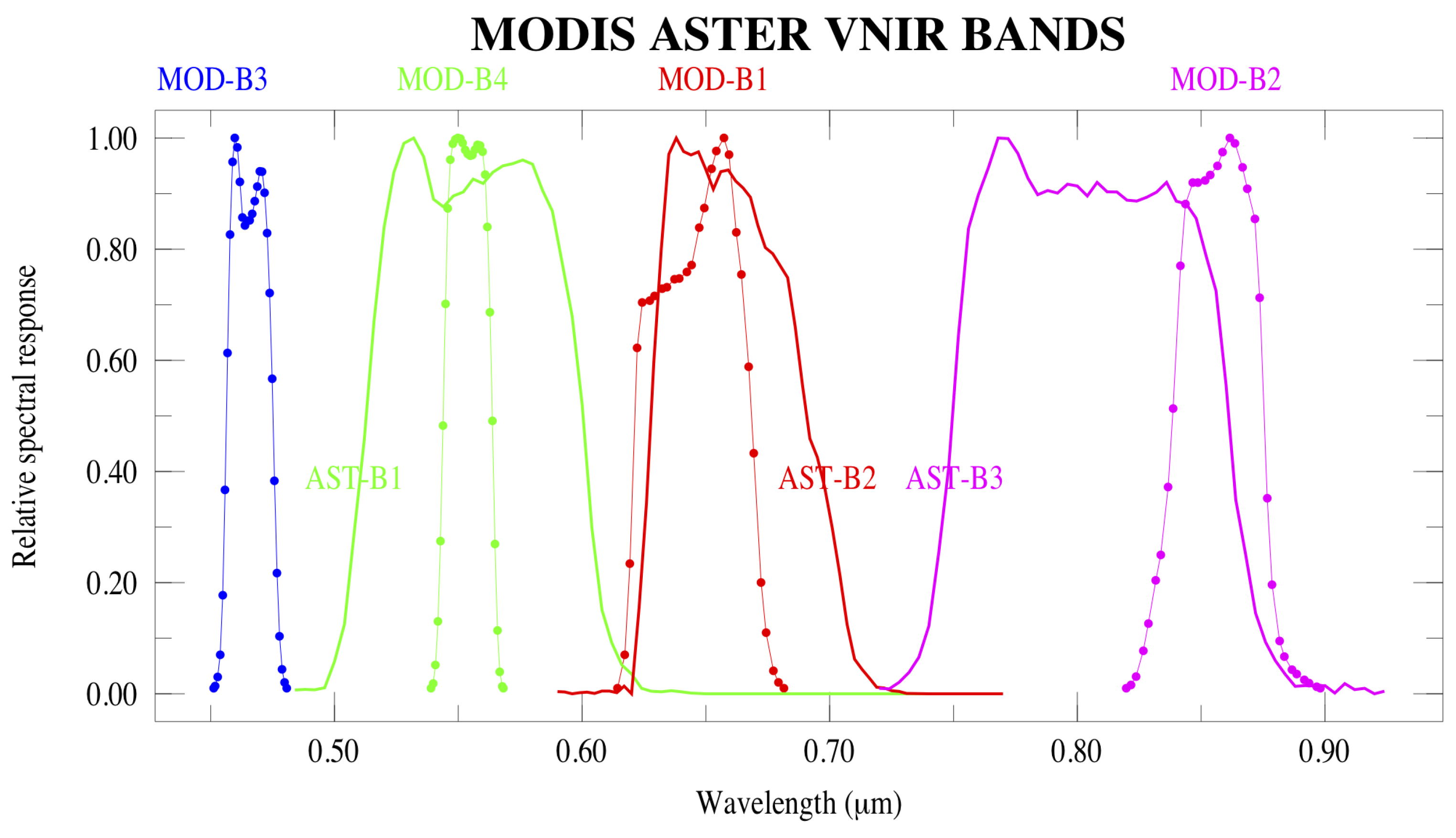
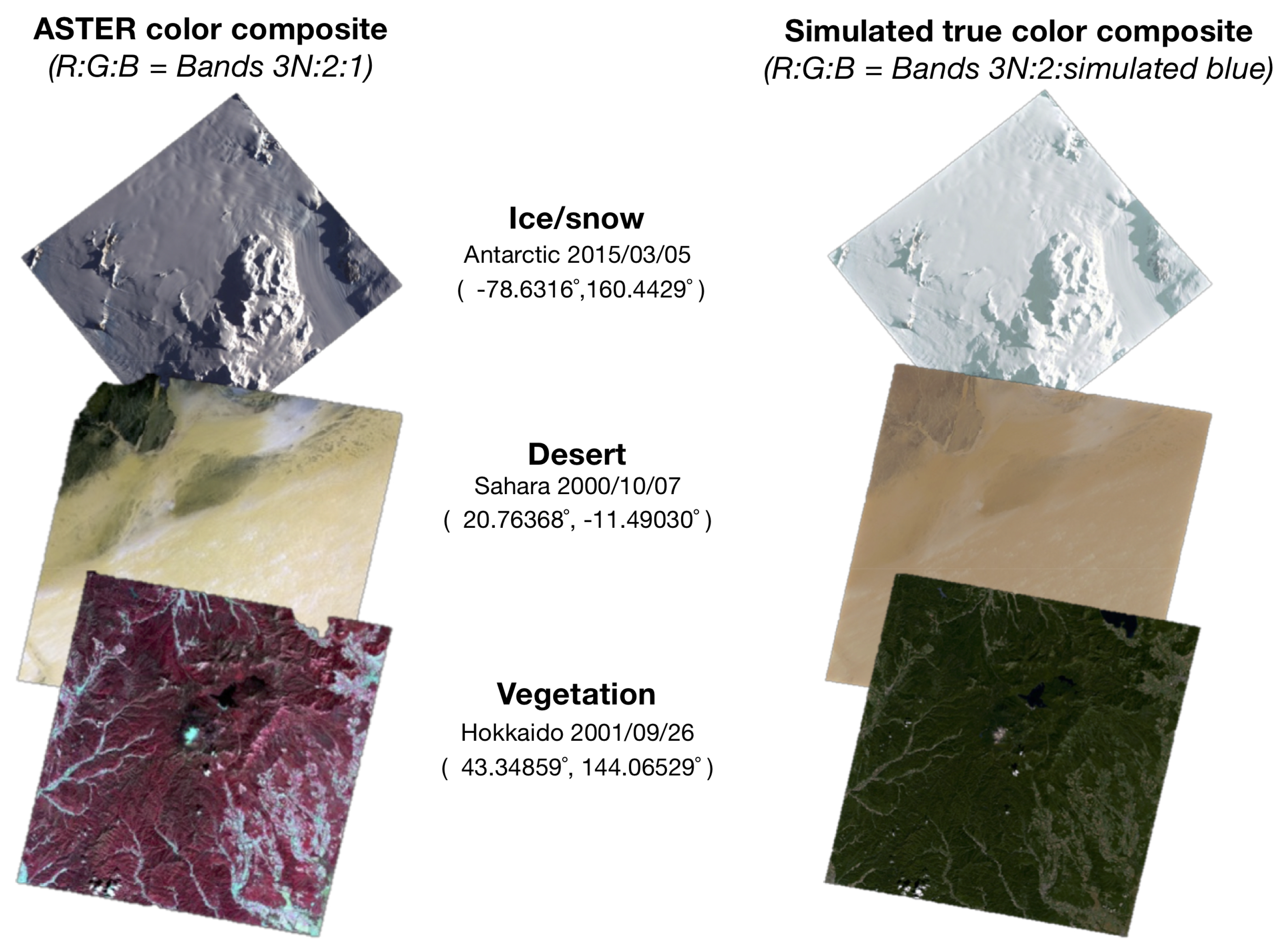
ASTER is a 15 m resolution, 14 bands multispectral instrument. It has been used for change detection, calibration, validation, and land surface studies from individual granules analysis [1]. However, the global monitoring of the Earth and ocean surfaces will be greatly helped by the integration of the satellite granule database from 2003 to 2012 into a unique natural color global mosaic, referred to as CLAMS (Color-Land ASTER MosaicS). The distributed ASTER granules cannot produce natural-color images, since ASTER sensors lack a blue visible band as illustrated by Figure 1. Generally, false color RGB composites are created by assigning red, green and blue to visible near infrared bands 3N, 2, and 1, respectively. However, ice/snow areas appear grey, desert areas yellow, and vegetation red, as illustrated on the left hand side of Figure 2.
In this work, we aim at constructing a global mosaic at 15 m of ground resolution, which blends our true-color visible ASTER images.
Several studies have addressed various ways of generating the simulated true color imagery for optical satellite sensors, which do not have a part of visible bands. Chen and Tsai [2] proposed spectral transformation techniques between Système Probatoire de l’Observation de la Terre (SPOT) false color image and Landsat-5 Thematic Mapper (TM) true color imagery. They used an unsupervised fuzzy c-means classifier and spectral control points. Knudsen [3] proposed a pseudo-natural color methodology for aerial imageries by using a simple least-squares adjusted linear model for the relationship between the blue band and the green, red and near-infrared (NIR) bands. This paper showed the possibilities of cost-efficiency by using the color-infrared (CIR) traditional photogrammetric products recorded by a traditional aerial camera. Patra et al. [4] developed spectral transformation techniques with spectral control points to IKONOS false-color imagery and natural color (simulated true color) imagery, and they evaluated their developed transformation method by using Quickbird, MODIS, Indian remote sensing satellite (IRS-P6) LISS-4, LISS-3, and AWiFS sensors. Huixi and Yunhao [5] applied the atmospheric correction algorithm, ATCOR to Landsat-7 ETM+, SPOT, and Terra ASTER imageries. They used the spectral similarity scale (SSS) method with a spectral library for generating pseudo natural color composites, and could obtain excellent results. Zhu et al. [6] developed a non-linear model based on a spectrum machine learning (SML) method with the spectral library, and they applied it to Landsat-7 ETM+, SPOT, and ASTER imageries. The atmospheric correction algorithm FLAASH from ENVI software was first applied, followed by the SML method to establish an implicit non-linear relationship between the blue band and other bands. The next-generation GOES-R advanced baseline imager (ABI) does not have a green band, and high-resolution atmospheric model simulations have been used to produce the ABI reflective band imagery required for true-color imagery [7,8]. Most researchers suggest that true-color algorithms are affected by sun-target-sensor geometry and atmospheric conditions.
There have been several efforts to construct cloud-free true color base-maps from moderate or high spatial resolution (less than 100 ) satellite data. ASTER has been operated over 19 years since Terra satellite launch in 1999. Thus, the huge available acquisitions database makes it possible to generate cloud-free global mosaics. The large number of ASTER image granules (about 780,000) used in this study were collected over many years, different seasons, and under varying vegetation and illumination conditions. Without the appropriate corrections, the resulting mosaic can appear as a patchwork of individual images. To avoid this, it deems necessary to apply atmospheric corrections and to smoothen seasonal effects. There have been several attempts of true-color mosaic constructions for various satellite optical sensors, mostly using adjustments of radiometric characteristics. Guindon [9] proposed radiometric adjustment for seamlessness mosaic of Landsat-5 MSS for northwestern Ontario area. Liew et al. [10] calculated solar zenith angle corrected radiances, and have used a brightness thresholding method to identify the best cloud-free and non-shadow pixels among the pixels from the multiple images at a given region. They successfully tested their mosaic technique with SPOT images acquired over the South East Asia region. Du et al. [11] applied a radiometric equalization techniques for representative pixel pairs in each overlap area, selected by means of a principal component analysis and calculation of linear correlation coefficients. They proved the methodology by mosaicking 6–7 Landsat-5 TM granules over the Boreal Ecosystem-Atmosphere Study (BOREAS) transect. Bindschadler et al. [12] generated a seamless cloud-free Landsat-7 ETM+ mosaic of Antarctica by radiometric adjustment. Roy et al. [13] produced a mosaic of the conterminous United States (CONUS) using 6521 Landsat-7 ETM+ imageries from December 2007 to November 2008. Choi et al. [14] developed the mosaic algorithm for high resolution images captured by Kompsat-2 sensor. This algorithm can be applied to different images affected by seasonal change, and is applicable to other high resolution optical sensor images. There exist two global mosaics, GeoCover2000 [15] (Landsat-7) and Landsat-8 VNIR maps [16], that have processed 30 Landsat images and pansharpened them to 15 . In summary, most attempts of generating mosaics of high resolution optical imageries were mostly carried out over regional areas, as the construction of a global cloud-free mosaic of high resolution imageries is extremely difficult due to the large amount of spatially and temporarily varying acquisitions.
We propose a protocol to assemble a true-color global mosaic from high-resolution ASTER imagery. The protocol first implies the construction of the missing ASTER blue band making use of the Moderate Resolution Imaging Spectroradiometer (MODIS) Terra instrument as it sits on board of the same satellite platform acquires time and space synchronized images with all visible bands, though at a lower spatial resolution (250–500 m). In 2012, we developed a first algorithm in which, after atmospheric corrections, the ASTER pseudo-blue band was constructed from a single artificial neural network (ANN), making it possible to generate ASTER granules in true color composite. These processed ASTER images are currently distributed by the AIST MADAS system as one of ASTER-VA products [17,18]. This first algorithm was not completely satisfactory and a couple of years ago, we decided to improve the blue color retrieval in particular over the ocean, as described in Section 2. The new retrieval algorithm this time uses a cloud of ANN’s, which preserve the finest details of the atmospheric components, such as dust, smoke and thin clouds.
The second key feature of the constructed CLAMS mosaic is that it is worldwide color-balanced, in the sense that the radiometric differences between the adjacent images introduced by the solar incident angle, atmosphere, and illumination condition are equalized. This is achieved by a novel color-balancing method for ASTER based on a MODIS reflectance reference library (FondsDeSol, FDS) proposed by Gonzalez et al. [19]. By automatically selecting appropriate color reference information from the FDS library according to the geographical scope and acquisition season information of the target images, the proposed approach provides effective solutions for eliminating color error propagations between adjacent granules over the globe. We will illustrate the rendered color quality of the mosaic in Section 3.1 and on the website http://newtec.univ-lille1.fr/LARGEMOSAICSFR/.
The third feature of the CLAMS mosaic is that it preserves the ASTER fine 15 structures across the various building steps, as demonstrated in Section 3.2.
2. Methodology for ASTER Blue Reflectance Reconstruction
In the entire document, all presented data correspond to reflectance values from MODIS L1B or ASTER L3A products to which minimum atmospheric corrections were applied to compensate for the Rayleigh scattering contribution, and correct for ozone according to the 6S radiative transfer code [20], with the same equations as in Ref. [21]. These corrected reflectances are denoted hereafter as . In all the figures, we present ASTER granules geometrically corrected to Plate Carrée projection (North oriented) within a bounding box of 75 × 75 , and we specify both the dates and geolocalization of their central points.
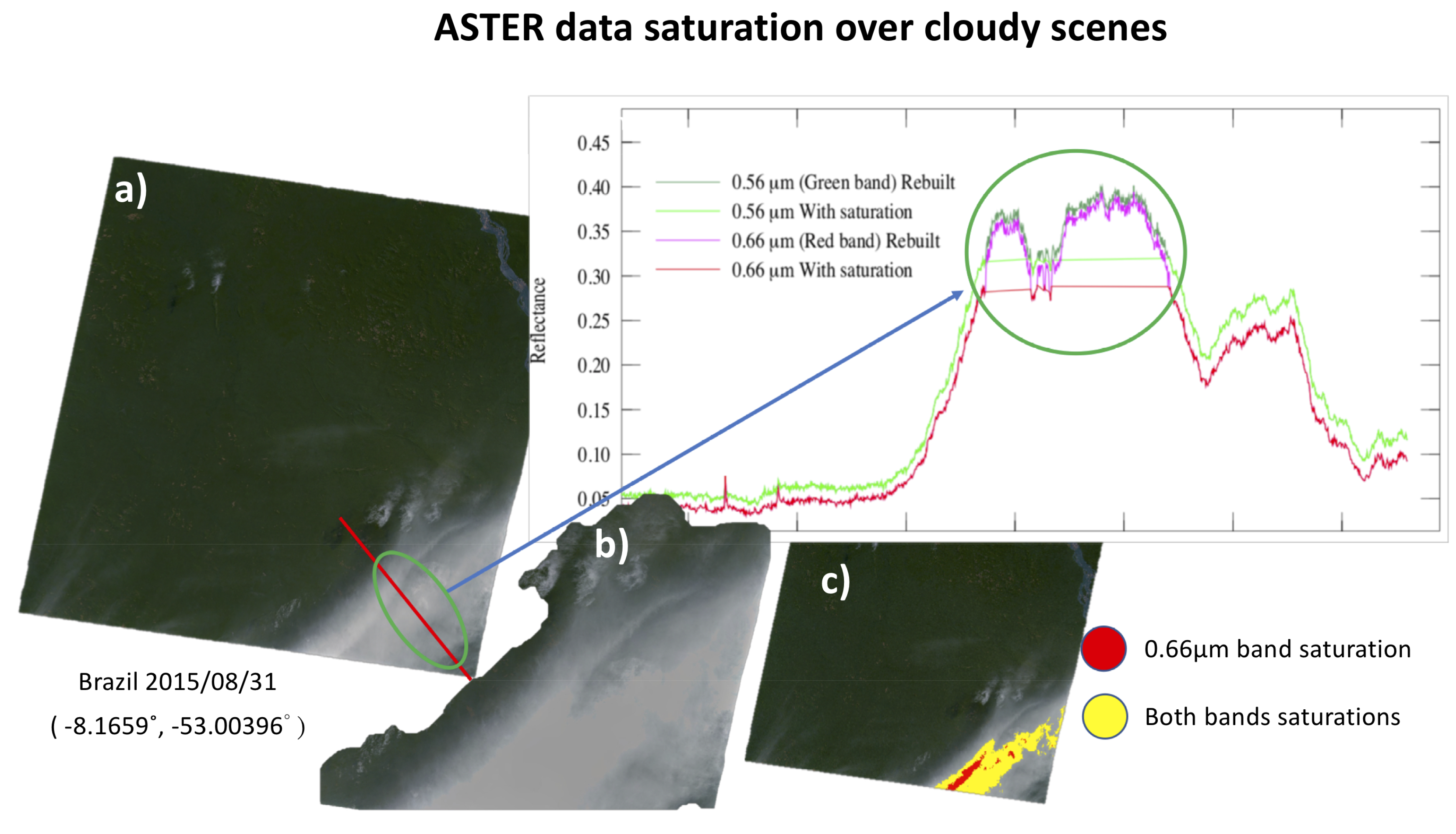
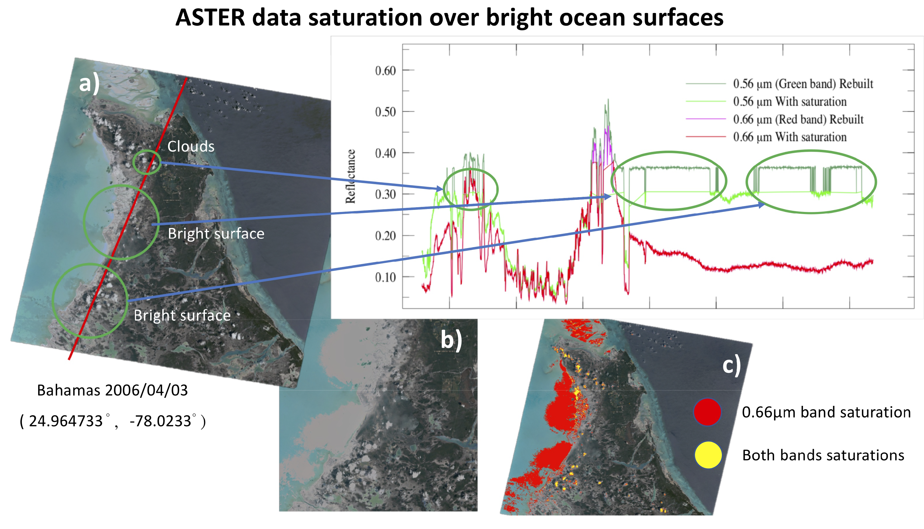
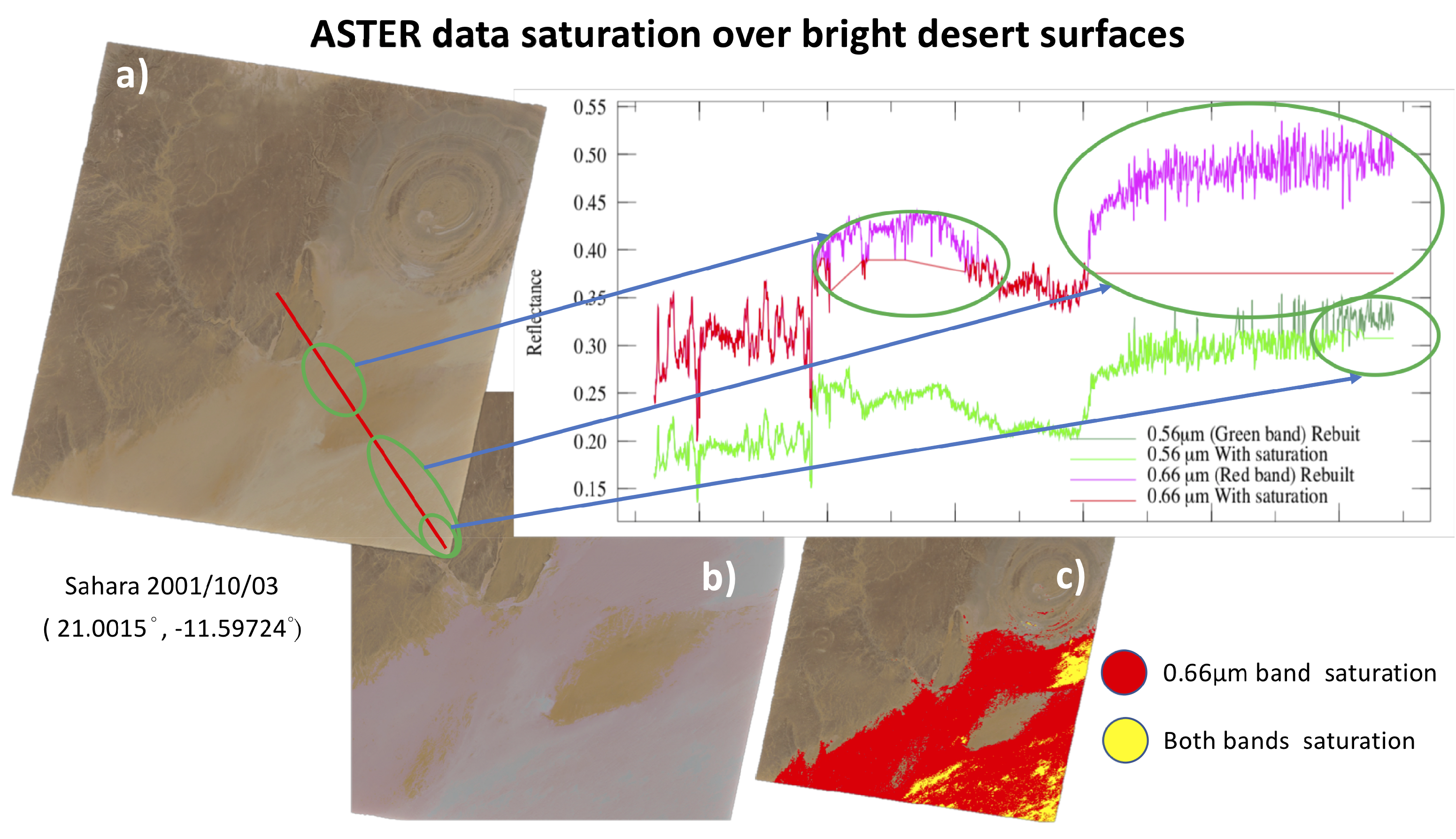
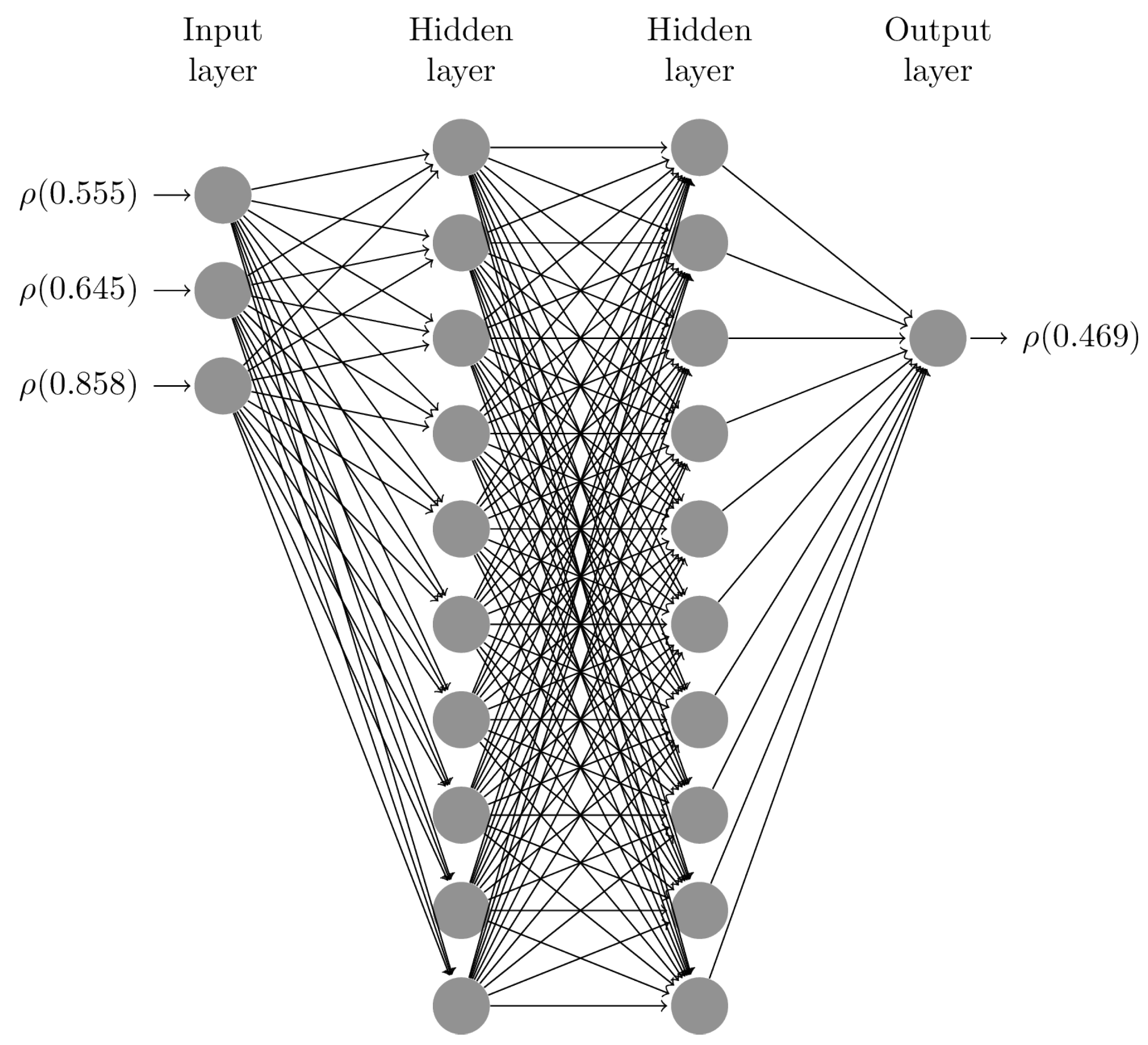
The ASTER granules suffer from two main defects. The first is linked to signal saturations in the and bands over bright surfaces as explained in Section 2.1, while the second corresponds to the missing band which is reconstructed with ANNs using MODIS reflectance data as detailed in Section 2.2. To train the ANN and to reconstruct the saturated ASTER pixels missing values we use as input data the 0.555, 0.645, and bands from MODIS and the blue band as target output data. To retrieve the ASTER blue band we use as input data the 0.56, 0.66, ASTER bands.
2.1. Reconstruction of Saturated ASTER Level1 Pixels
In the process of correcting the bright surface saturation we do not expect to retrieve the real reflectances but simply to create reasonable values giving true color composites close to reality. Saturated values only appear for the 0.56 and bands (noted and ). A correction model was empirically determined using MODIS reflectances over the ASTER saturated areas. It turned out that simple first and second-order polynomial functions of the () reflectances could be used to assign unsaturated reflectance values and , as detailed in Table 1.
2.2. ANN to Reconstruct ASTER Blue Reflectances
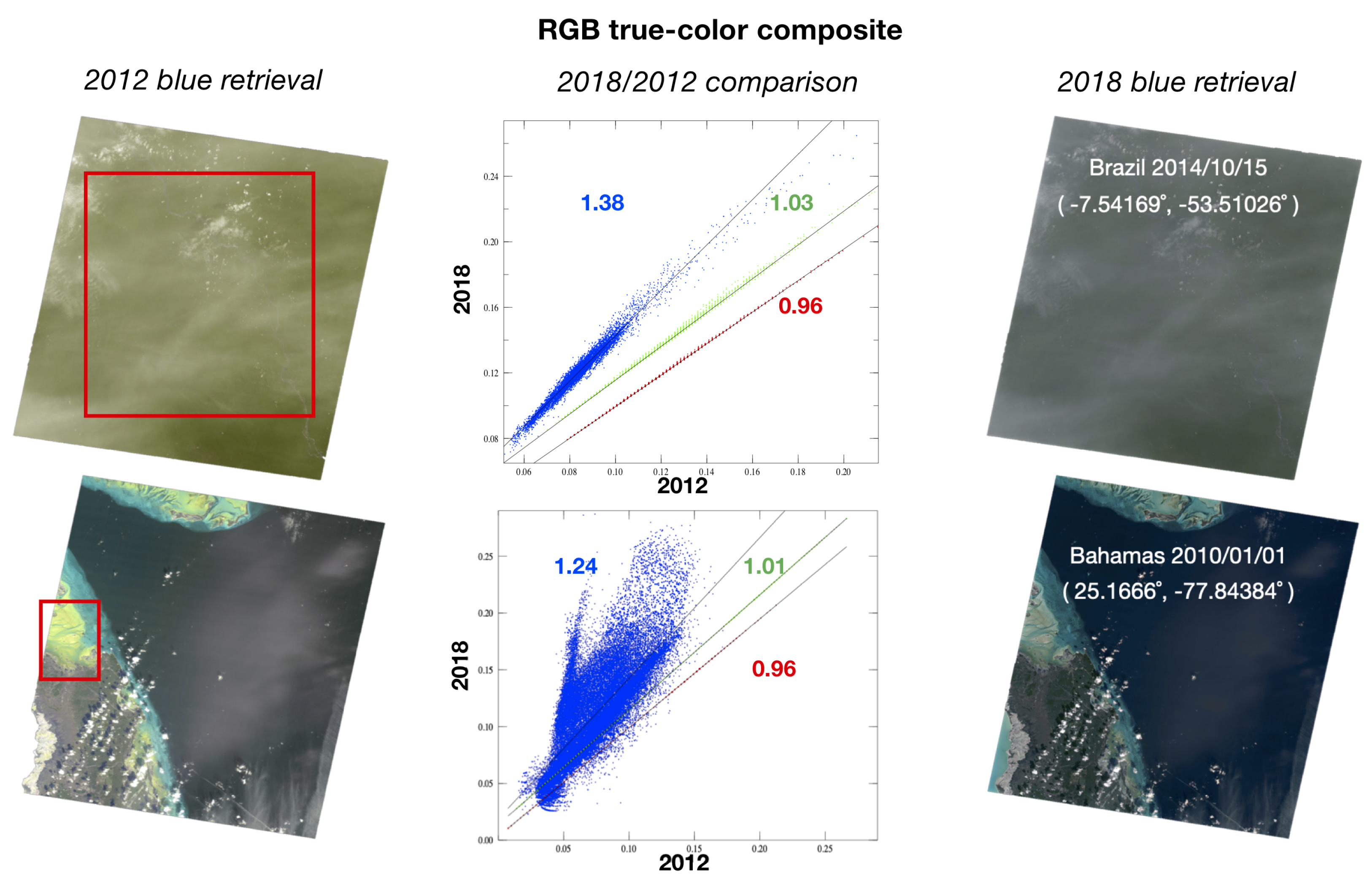
Fine-tuning the parameters of an ANN (Stuttgart Neural Network Simulator (SNNS) [22]) to faithfully reconstruct ASTER blue reflectances turned out to be a tricky process. In 2012, we designed an ANN that used for the training inputs the 3 MODIS 0.555, 0.645, bands (spectrally close to the VNIR ASTER bands, 0.56, 0.66, ), and the blue MODIS band at as target values. This ANN is a fully connected feedforward network [23]. The ANN topology we present yields the best blue retrieval out of many tests we carried out. It consists of two hidden layers with 10 nodes each (See Figure 6). The training data set used a selection of about fifty MODIS granules for which we hand-selected representative areas such as water, ocean colors, deserts, rocks, white and bright surfaces, etc. Once trained, the network was tested on various MODIS granules and the training ANN data set was enlarged with those showing inaccurate (poor correlation with respect to MODIS real blue reflectances) reconstructed blue values. However, the blue retrieval was not fully accurate, yielding yellow colors over hazy areas and bright reefs as illustrated by the examples on the left hand side of Figure 7.
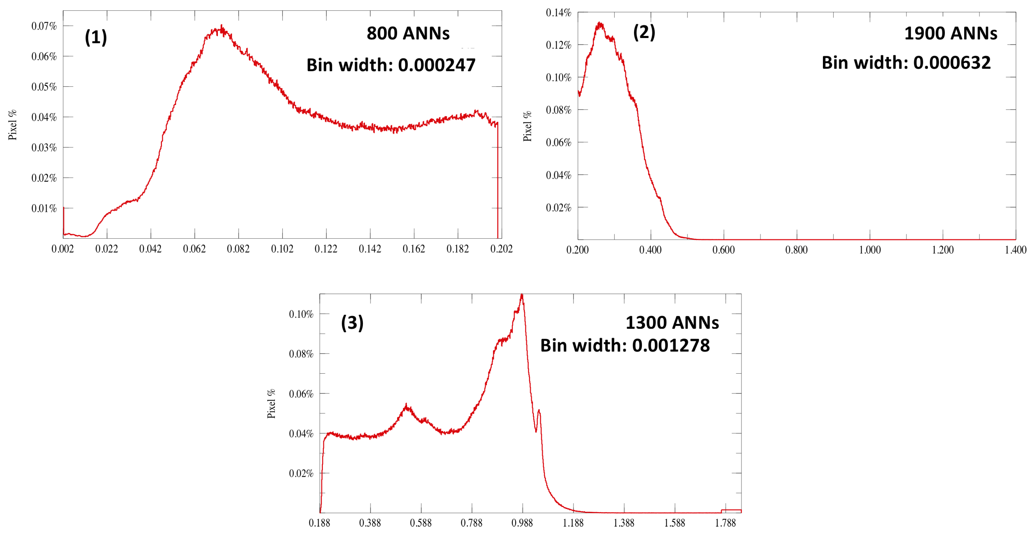
Based on our recent experience with ANNs design for aerosol optical depth retrievals [21], we found out that ANNs training and accuracy are improved if applied to specific classes of reflectance values. Thus, our new algorithm uses MODIS values that are classified into three groups according to the values , defining two main areas, the first one corresponding to water, dark areas and vegetation (), the second one to desert areas (). The third group encompasses the brightest cloudy pixels selected by according to the following three-fold tests:
The histograms of the three groups are drawn in Figure 8. Each of the three histograms are split to define subclasses of pixel values defining the inputs of ANNs. The determination of the number of data by classes (bins) was carried out in successive stages by monitoring both the convergence of the networks and the quality of the blue retrieval over about one hundred MODIS granules that compose the training data sets. It soon became clear that the first group requires a more precise division (800 networks) and converges with an average number of 4000 pixels per bin. In group 2, the subdivision is wider with 1900 networks and an average number of 2200 pixels per bin was necessary. The third group requires 1300 networks with an average number of 3200 pixels per bin. Figure 9 demonstrates how the histogram classification is used to split the MODIS data. For each bin, a dedicated ANN with a feedforward topology, with the same architecture as before (3 inputs, 2 hidden layers with 10 nodes each, and 1 output value, see Figure 6), is designed. Altogether an ensemble of 4000 ANNs is trained. The training dataset was enlarged to about one hundred MODIS granules.
For the retrieval, the three ASTER bands (0.56, 0.66, ) are scaled to match the MODIS ones (0.555, 0.645, ) as:
the coefficients being determined from linear regressions.
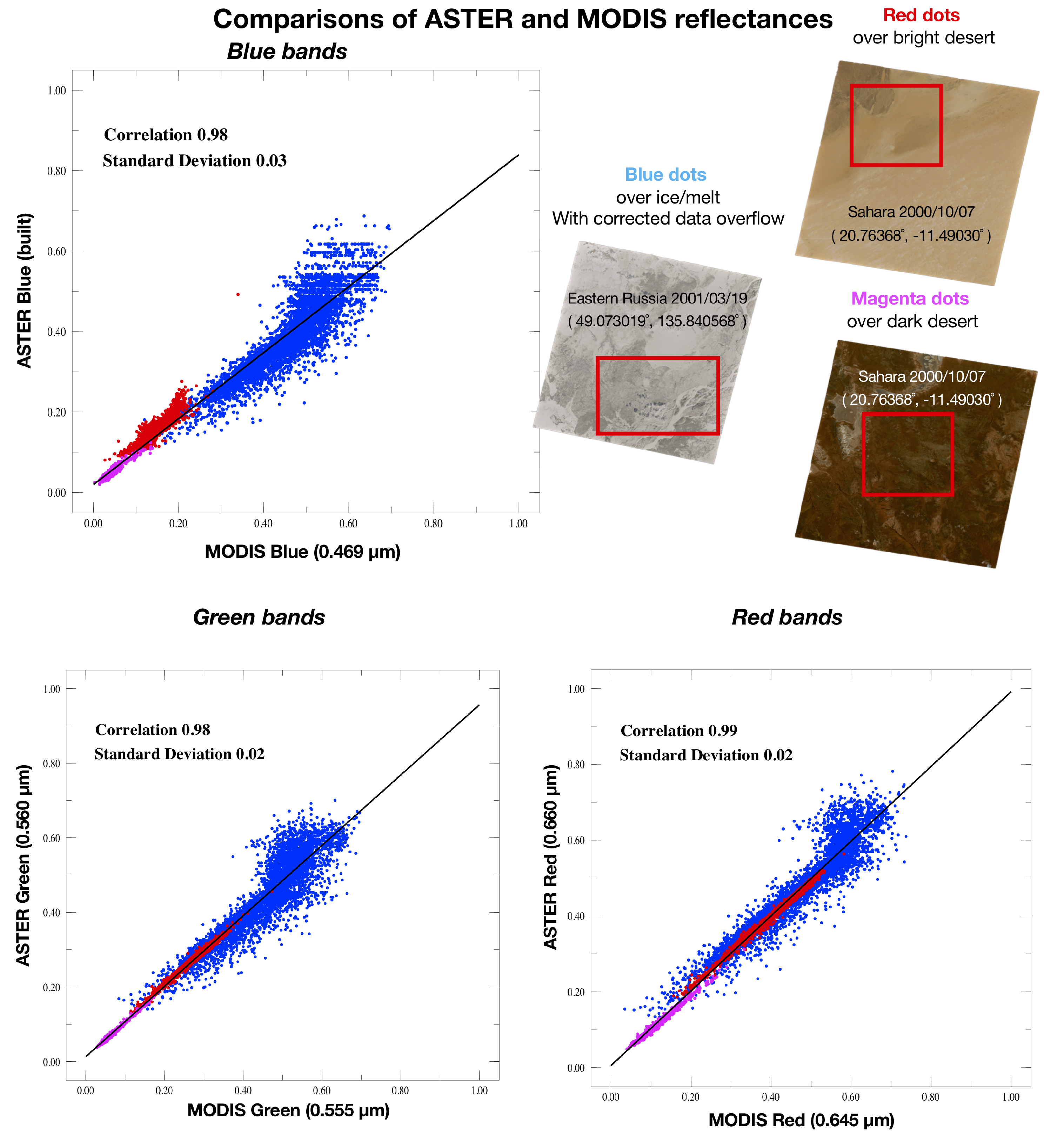
The central panel of Figure 7 demonstrates that the 2018 blue retrieval algorithm yields enhanced blue reflectances, improving the final image rendering. Furthermore, the absolute quality of the 2018 blue reconstruction is proven by Figure 10 showing the excellent correlations (at least 0.98 with low standard deviations, max of 0.03) between all three bands of ASTER and MODIS. This is further highlighted by Figure 11 where a comparable agreement is found with Landsat-8 OLI L1T products which holds a real blue channel. This Landsat-8 L1T were obtained via the USGS EarthExplorer.
In order to preserve the spectral response of ASTER instrument, the red and green bands of the final visible composite are the ASTER original measurements, while the blue is reconstructed from the cloud of ANNs. As the MODIS and ASTER bands response are slightly shifted (See Figure 1), one can observe in Figure 12 subtle differences for red and green areas in the final color rendering of the natural ASTER composite with respect to MODIS.
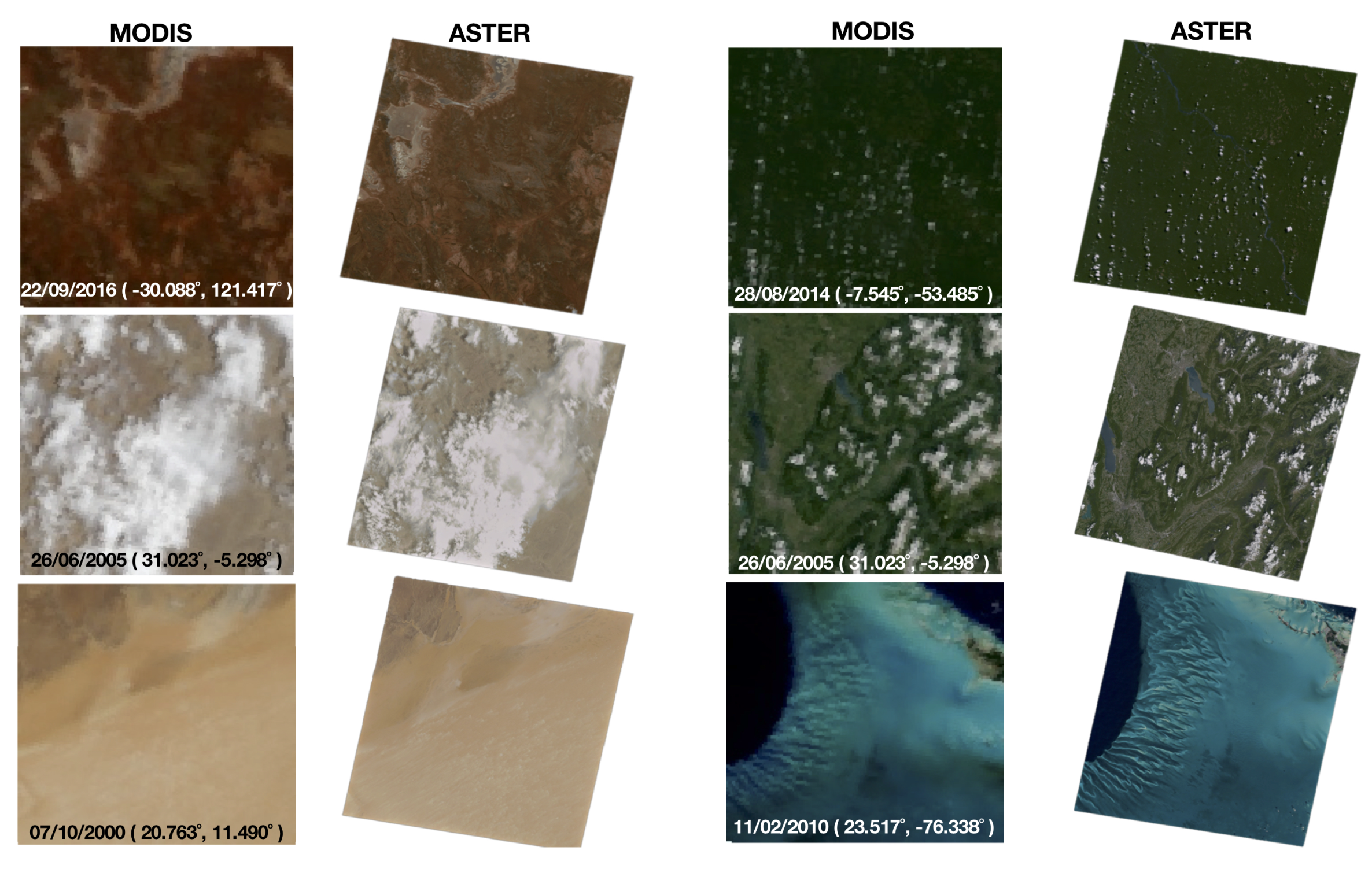
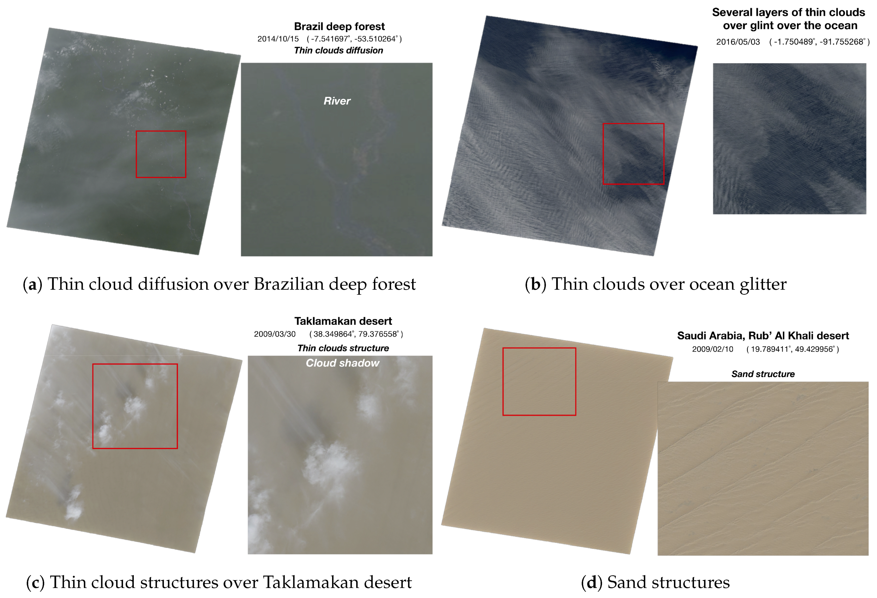
To further illustrate the accuracy of the blue reconstruction, we present in Figure 13, examples of heterogeneous natural-color reconstructions. The final results preserve the 15 m ASTER sensitivity, as we notably recognize the signatures of thin clouds on both dark (Figure 13a,b) and bright backgrounds (Figure 13c) with their shadows, as well as the fine patterns of bright sand dunes in deserts (Figure 13d).
3. Building a Global Mosaic
The protocol to construct the CLAMS global mosaic released in 2012 has involved the scanning of the whole distributed ASTER portfolio from 2003 onwards to define a classification algorithm that sorts images with respect to their temporal distance to a seasonal reference date, but also with increasing degree of cloudiness as to minimize cloudy granules. About 780,000 granules where analyzed from where 70% were downloaded and colorized, while 40% contribute to the final mosaic.
3.1. Color-Matching of ASTER Granules to FondsDeSol Reference
In order to construct a seamless global mosaic image, radiometric and phenomenological scene differences have to be minimized across space and time. Helmerand and Ruefenacht [24] used histogram matching of adjacent scenes to build small-size regional mosaics, but this approach leads to increasingly growing bias when applied to large-scale areas. The availability of a world-wide cloud-free surface reflectance database FondsDeSol [19] centered at the end of august is used as reference to equalize the ASTER granules over the whole Earth.
To achieve the color equalization of the ASTER RGB bands and remove as far as possible bidirectional effects and seasonal changes, we have used the iterative distribution transfer (IDT) algorithm proposed by Pitié et al. [25], which allows within few iterations, typically less than 10, an excellent color match to the FondsDeSol reference. It is noteworthy that this colorization process allows to partially dehaze ASTER granules that are blurred by the atmospheric aerosols. An example is displayed in Figure 14, which presents in subset Figure 14 (1) patched natural color ASTER granules tainted by the atmospheric components. Figure 14 (2) shows the same patch colorized by the IDT process, the only visible transitions being that of the granules boundaries. Indeed, seasonal effects are smoothened but may be still be slightly visible when the land surface is significantly altered across various seasons (field structures, forest, rivers, etc.).
3.2. Seamless ASTER Granules Blending
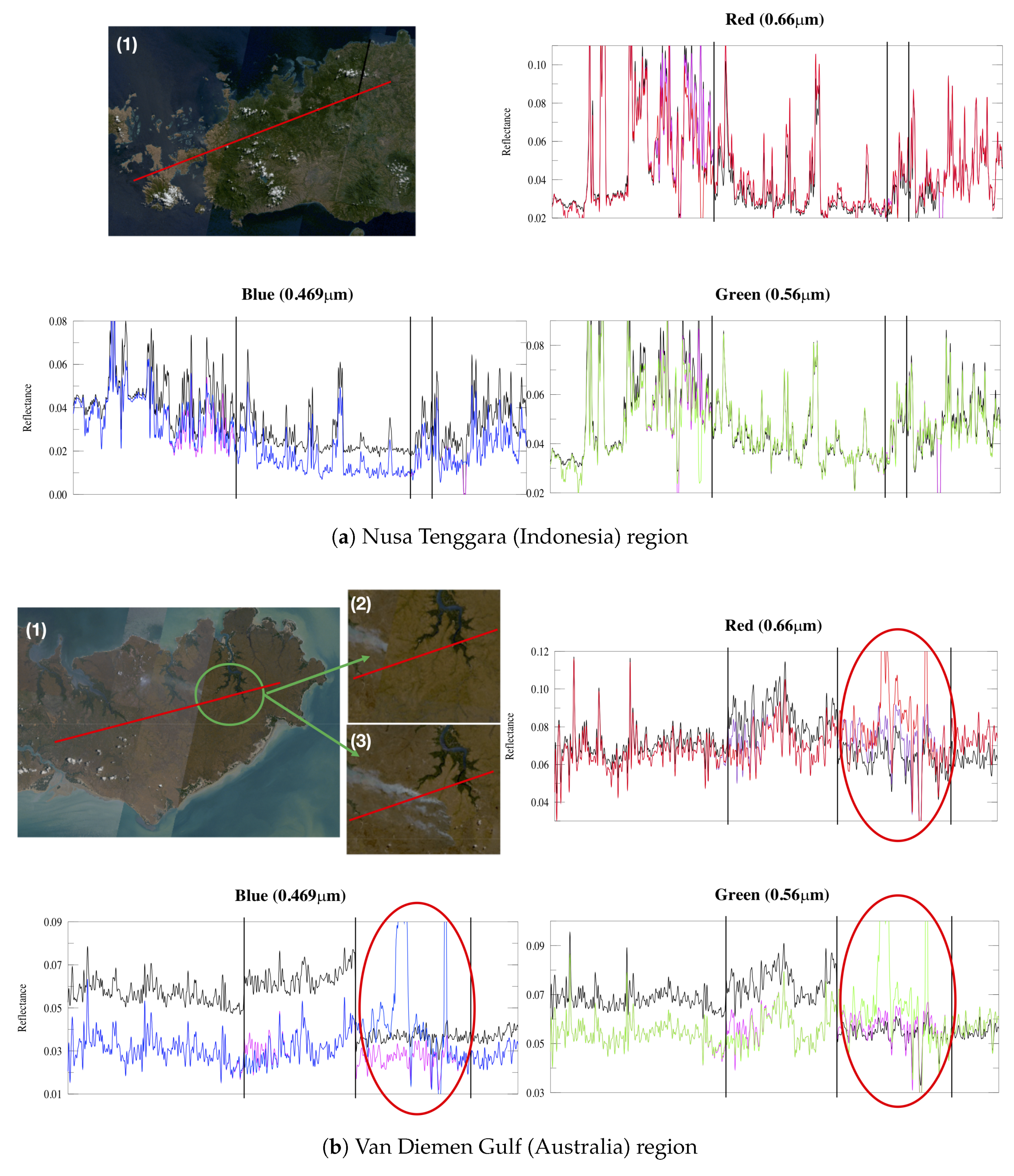
To create seamless mosaics, we relied on an effective methodology using the Laplacian pyramid-based algorithm introduced by Burt and Adelson [26]. Multi-scale Gaussian pyramid representations of the overlapping areas of the patched granules are used to merge all the spatial structural details at the 15 resolution, the color matching being already achieved by the FondsDeSol color equalization preceding step. Figure 15 illustrates the reflectance values over transects of two different surface types in the Nusa Tenggara (Indonesia) and Van Diemen Gulf (Australia). The black curves represent the original ASTER natural color granules, the magenta or purple lines refer to the values across IDT colorized granules, while the R,G,B curves correspond to the final results after pyramid blending. Note that the different steps shift the reflectance values but preserve the fine structures of the original data. In Figure 15a, the colorization and blending effects are minor across the granules boundaries (vertical black lines). In Figure 15b we have highlighted with red circles large changes in the reflectance values between the two last steps of the mosaic process (IDT and blending). In this example the blending step (displayed in the (3) inset) brings in thin smoke plumes from the background image (https://earthexplorer.usgs.gov/).
3.3. Filling the Gaps
For limited numbers of very small areas, where we did not find any suitable ASTER granules, we patched the mosaic with less than 100 Landsat-7 ETM+ granules processed by NASA/JPL CalTech, which is derived from GeoCover2000 [15]. These were color-equalized with the IDT algorithm and merged into the mosaic with the pyramid blending method.
3.4. Distribution of the Mosaic
Partial mosaics samples can be seen on http://newtec.univ-lille1.fr/LARGEMOSAICSFR/ with a web interface that allows to visualize and zoom into several subsets of the global mosaic, with the 2012 blue algorithm (France, Saudi Arabia), and the 2018 blue algorithm (Australia, Indonesia, South Africa, Bahamas, Antarctic). The global mosaic with the 2012 blue algorithm will be available on the https://gbank.gsj.jp/madas/?lang=en web-platform in 2019, while the latest higher quality one shall be also available in the near future.
4. Conclusions and Future Work
This work is the first world-wide mosaic of ASTER images in natural colors. Two main problems of the distributed data have been tackled, namely the saturation over bright surfaces, and most importantly the lack of a blue band. The latter was reconstructed using a large cloud of ANNs trained on MODIS reflectance values, improving the blue rendering with respect to the 2012 version. The granules with the 2012 version are readily available on the https://gbank.gsj.jp/madas/?lang=en web-platform, while the latest higher quality ones shall be available in the near future. The availability of true-color ASTER granules is by itself relevant to help comparisons with other huge high-resolution database as Landsat, in particular to monitor surface changes.
The construction of the mosaic implies to harmonize the colors of spatially and temporarily separated granules and to fusion them with seamless blending algorithms. We have demonstrated that the various steps preserve the 15 spatial structures of the original ASTER images. The created global mosaic is a real 15 resolution mosaic that can serve as a reference to validate the quality of other global maps [15,16]. The presented mosaic protocol with the improved blue retrieval will shortly be applied to create a revised version of the ASTER mosaic. The proposed algorithmic protocol has processed several hundred thousands ASTER images and its robustness and modularity can be adapted to similar sensors with enormous image libraries, such as SPOT.
Author Contributions
Conceptualization, L.G.; Methodology, L.G. and V.V.; Software, L.G. and V.V.; Supervision, H.Y.; Validation, L.G. and H.Y.; Writing—original draft, L.G., V.V. and H.Y.
Funding
This research received no external funding.
Acknowledgments
The research for the ASTER in this paper was partially supported by the Ministry of Economy, Trade and Industry in Japan. Original ASTER imagery is provided by “NASA/METI/AIST/Japan Spacesystems, and U.S./Japan ASTER Science Team”. All MODIS products are courtesy of the online Data Pool at the NASA Land Processes Distributed Active Archive Center (LP DAAC), USGS/Earth Resources Observation and Science (EROS) Center, Sioux Falls, South Dakota.
Conflicts of Interest
The authors declare no conflict of interest.
References
- Abrams, M.; Hook, S.; Ramachandran, B. ASTER User Handbook, Version 2; Jet Propulsion Laboratory: Pasadena, CA, USA, 2002. Available online: http://asterweb.jpl.nasa.gov/content/03_data/04_Documents/aster_user_guide_v2.pdf (accessed on 3 January 2019).
- Chen, C.F.; Tsai, H. A spectral transformation technique for generating SPOT natural color image. In Proceedings of the 19th Asian Conference on Remote Sensing, Manila, Philippines, 16–20 November 1998. [Google Scholar]
- Knudsen, T. Technical Note: Pseudo natural color aerial imagery for urban and suburban mapping. Int. J. Remote Sens. 2005, 26, 2689–2698. [Google Scholar] [CrossRef]
- Patra, S.K.; Shekher, M.; Solanki, S.S.; Ramachandran, R.; Krishnan, R. A technique for generating natural colour images from false colour composite images. Int. J. Remote Sens. 2006, 27, 2977–2989. [Google Scholar] [CrossRef]
- Huixi, X.; Yunhao, C. A technique for simulating pseudo natural color images based on spectral similarity scales. IEEE Geosci. Remote Sens. 2012, 9, 70–74. [Google Scholar] [CrossRef]
- Zhu, C.; Luo, J.; Ming, D.; Shen, Z.; Li, J. Method for generating SPOT natural-colour composite images based on spectrum machine learning. Int. J. Remote Sens. 2012, 33, 1309–1324. [Google Scholar] [CrossRef]
- Hillger, D.W.; Grasso, L.; Miller, S.D.; Brummer, R.; DeMaria, R.J. Synthetic advanced baseline imager true-color imagery. J. Appl. Remote Sens. 2011, 5, 053520. [Google Scholar] [CrossRef]
- Miller, S.D.; Schmidt, C.C.; Schmit, T.J.; Hillger, D.W. A case for natural colour imagery from geostationary satellites, and an approximation for the GOES-R ABI. Int. J. Remote Sens. 2012, 33, 3999–4028. [Google Scholar] [CrossRef]
- Guindon, B. Assessing the radiometric fidelity of high resolution satellite image mosaics. ISPRS J. Photogramm. Remote Sens. 1997, 52, 229–243. [Google Scholar] [CrossRef]
- Liew, S.C.; Li, M.; Kwoh, L.K.; Chen, P.; Lim, H. “Cloud-free” multi-scene mosaics of SPOT images. In Proceedings of the IGARSS ’98—1998 IEEE International Geoscience and Remote Sensing, Seattle, WA, USA, 6–10 July 1998; Volume 2, pp. 1083–1085. [Google Scholar] [CrossRef]
- Du, Y.; Cihlar, J.; Beaubien, J.; Latifovic, R. Radiometric normalization, compositing, and quality control for satellite high resolution image mosaics over large areas. IEEE T. Geosci. Remote Sens. 2001, 39, 623–634. [Google Scholar] [CrossRef]
- Bindschadler, R.; Vornberger, P.; Fleming, A.; Fox, A.; Mullins, J.; Binnie, D.; Paulsen, S.J.; Granneman, B.; Gorodetzky, D. The Landsat image mosaic of Antarctica. Remote Sens. Environ. 2008, 112, 4214–4226. [Google Scholar] [CrossRef]
- Roy, D.P.; Ju, J.; Kline, K.; Scaramuzza, P.L.; Kovalskyy, V.; Hansen, M.; Loveland, T.R.; Vermote, E.; Zhang, C. Web-enabled Landsat Data (WELD): Landsat ETM+ composited mosaics of the conterminous United States. Remote Sens. Environ. 2010, 114, 35–49. [Google Scholar] [CrossRef]
- Choi, J.; Jung, H.S.; Yun, S.H. An efficient mosaic algorithm considering seasonal variation: Application to KOMPSAT-2 satellite images. Sensors 2015, 15, 5649–5665. [Google Scholar] [CrossRef] [PubMed]
- Plesea, L. Remote access to very large image repositories, a high performance computing perspective. In Proceedings of the Earth-Sun System Technology Conference, Adelphi, MD, USA, 28–30 June 2005. [Google Scholar]
- Descartes Maps. Available online: http://www.descarteslabs.com/maps.html (accessed on 3 January 2019).
- AIST “ASTER-VA”, Value-Added Satellite Observation Data, Provided at No Cost. Available online: https://gbank.gsj.jp/madas/ (accessed on 3 January 2019).
- Obata, K.; Tsuchida, S.; Yamamoto, H.; Thome, K. Cross-calibration between ASTER and MODIS visible to near-infrared bands for improvement of ASTER radiometric calibration. Sensors 2017, 17, 1793. [Google Scholar] [CrossRef] [PubMed]
- Gonzalez, L.; Bréon, F.M.; Caillault, K.; Briottet, X. A sub km resolution global database of surface reflectance and emissivity based on 10-years of MODIS data. ISPRS J. Photogramm. Remote Sens. 2016, 122, 222–235. [Google Scholar] [CrossRef]
- Vermote, E.; Kotchenova, S.; Tanré, D.; Deuzé, J.; Herman, M.; Roger, J.C.; Morcrette, J. 6SV Code. 2015. Available online: http://6s.ltdri.org (accessed on 20 February 2019).
- Gonzalez, L.; Briottet, X. North Africa and Saudi Arabia Day/Night Sandstorm Survey (NASCube). Remote Sens. 2017, 9, 896. [Google Scholar] [CrossRef]
- Zell, A.; Mache, N.; Hübner, R.; Mamier, G.; Vogt, M.; Schmalzl, M.; Herrmann, K.U. SNNS (Stuttgart Neural Network Simulator). In Neural Network Simulation Environments; Springer: Boston, MA, USA, 1994; pp. 165–186. [Google Scholar]
- Miikkulainen, R. Topology of a Neural Network. In Encyclopedia of Machine Learning; Sammut, C., Webb, G.I., Eds.; Springer: Boston, MA, USA, 2010; pp. 988–989. [Google Scholar] [CrossRef]
- Helmer, E.H.; Ruefenacht, B. Cloud-Free Satellite Image Mosaics with Regression Trees and Histogram Matching. Photogramm. Eng. Remote Sens. 2005, 71, 1079–1089. [Google Scholar] [CrossRef]
- Pitié, F.; Kokaram, A.C.; Dahyot, R. Automated colour grading using colour distribution transfer. Comput. Vis. Image Underst. 2007, 107, 123–137. [Google Scholar] [CrossRef]
- Burt, P.J.; Adelson, E.H. A Multiresolution Spline with Application to Image Mosaics. ACM Trans. Graph. 1983, 2, 217–236. [Google Scholar] [CrossRef]
Sample Availability: Examples of the global natural colored mosaic are available on the http://newtec.univlille1.fr/LARGEMOSAICSFR/ website. |
Figure 1.
Normalized spectral response functions of ASTER (solid line) and MODIS (dotted lines) VNIR bands.
Figure 1.
Normalized spectral response functions of ASTER (solid line) and MODIS (dotted lines) VNIR bands.

Figure 2.
Examples of ASTER granules over different areas (ice/snow, desert, vegetation) rendered either with the false color composite (R:G:B = Bands 3N:2:1) on the left hand side, or with the simulated true color composite (R:G:B = Bands 3N:2:simulated blue) on the right hand side.
Figure 2.
Examples of ASTER granules over different areas (ice/snow, desert, vegetation) rendered either with the false color composite (R:G:B = Bands 3N:2:1) on the left hand side, or with the simulated true color composite (R:G:B = Bands 3N:2:simulated blue) on the right hand side.

Figure 3.
Visualization of the saturation corrections over cloudy areas: (a) final true color composite; (b) original saturated granule; (c) mask of the saturated areas (in red for the band and in yellow for both 0.56 and bands).
Figure 3.
Visualization of the saturation corrections over cloudy areas: (a) final true color composite; (b) original saturated granule; (c) mask of the saturated areas (in red for the band and in yellow for both 0.56 and bands).

Figure 4.
Visualization of the saturation corrections over the ocean: (a) final true color composite; (b) original saturated granule; (c) mask of the saturated areas (in red for the band and in yellow for both 0.56 and bands).
Figure 4.
Visualization of the saturation corrections over the ocean: (a) final true color composite; (b) original saturated granule; (c) mask of the saturated areas (in red for the band and in yellow for both 0.56 and bands).

Figure 5.
Visualization of the saturation corrections over desert areas: (a) final true color composite; (b) original saturated granule; (c) mask of the saturated areas (in red for the band and in yellow for both 0.56 and bands).
Figure 5.
Visualization of the saturation corrections over desert areas: (a) final true color composite; (b) original saturated granule; (c) mask of the saturated areas (in red for the band and in yellow for both 0.56 and bands).

Figure 6.
Topology of the ANN with one input layer taking 0.555, 0.645, and reflectance values, the .
Figure 6.
Topology of the ANN with one input layer taking 0.555, 0.645, and reflectance values, the .

Figure 7.
Comparisons of ASTER granules obtained with the blue retrieval algorithms of 2012 (left) and 2018 (right). The center panel shows the correlations between the reflectance values collected within the red boxes, obtained with the 2012 (x-axis) and 2018 (y-axis) algorithms.
Figure 7.
Comparisons of ASTER granules obtained with the blue retrieval algorithms of 2012 (left) and 2018 (right). The center panel shows the correlations between the reflectance values collected within the red boxes, obtained with the 2012 (x-axis) and 2018 (y-axis) algorithms.

Figure 8.
Histograms of the three groups of MODIS data to define the ANNs inputs.

Figure 9.
Scheme illustrating the pixel classification of the training (a) MODIS data. Subfigures (b–d) display the selected pixels (unselected pixels in magenta) sorted into classes (bins) by the (e–g) histograms. In histogram (e), we select 10 bins from 0.072 < x < 0.078 (h), and display the spatial location of two bins as green and red dots in the zoom (i). The MODIS reflectance values within a bin are used as inputs of the dedicated ANN (feedforward ANN with 3 inputs, 2 hidden layers with 10 nodes each, and 1 output) to retrieve the blue band.

Figure 10.
Correlations between ASTER and MODIS reflectance values for the red, green and blue bands, across several surfaces (selected within the red boxes), as ice/melt areas (blue dots), bright desert areas (red dots), and dark desert areas (magenta dots).
Figure 10.
Correlations between ASTER and MODIS reflectance values for the red, green and blue bands, across several surfaces (selected within the red boxes), as ice/melt areas (blue dots), bright desert areas (red dots), and dark desert areas (magenta dots).

Figure 11.
Correlations between ASTER (blue), OLI (red) and MODIS reflectance values (selected within the red box) for the red, green and blue bands over a desert area.
Figure 11.
Correlations between ASTER (blue), OLI (red) and MODIS reflectance values (selected within the red box) for the red, green and blue bands over a desert area.

Figure 12.
Comparison between the color rendering by MODIS on the left and ASTER (natural color simulated) on the right.
Figure 12.
Comparison between the color rendering by MODIS on the left and ASTER (natural color simulated) on the right.

Figure 13.
Examples of heterogeneous reconstructions of natural-color ASTER granules in different areas. The left figure is the ASTER granule and the right inset a zoom into the red box.
Figure 13.
Examples of heterogeneous reconstructions of natural-color ASTER granules in different areas. The left figure is the ASTER granule and the right inset a zoom into the red box.

Figure 14.
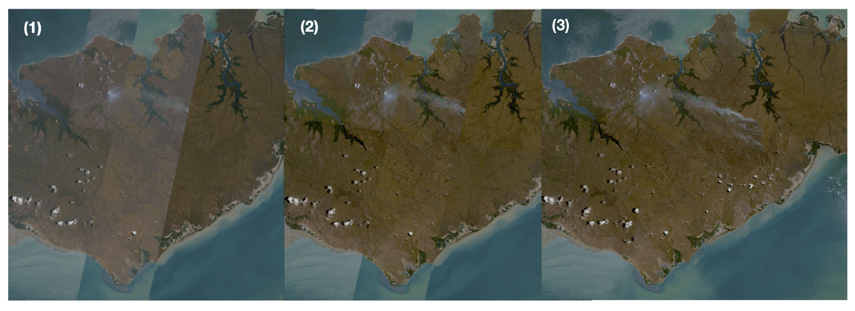
Illustrations of the ASTER mosaic quality over Van Diemen Gulf (Australia): (1) patch of the natural color ASTER granules; (2) patch the IDT colorized granules; (3) seamless blending of IDT colorized granules.
Figure 14.
Illustrations of the ASTER mosaic quality over Van Diemen Gulf (Australia): (1) patch of the natural color ASTER granules; (2) patch the IDT colorized granules; (3) seamless blending of IDT colorized granules.

Figure 15.
RGB reflectance values across the red marked transects; black lines refer to the patch of the natural color ASTER granules (1); magenta lines to the patch of IDT colorized granules (2); red, green, and blue lines correspond to the final reflectance values in the seamless CLAMS mosaic (3). Black vertical lines mark the granules boundaries.


Table 1.
Polynomial expansions for the saturation correction of bands ( ), ( ) using ( ).
| Ocean Colors | |
| Desert | |
| Clouds | |
© 2019 by the authors. Licensee MDPI, Basel, Switzerland. This article is an open access article distributed under the terms and conditions of the Creative Commons Attribution (CC BY) license (http://creativecommons.org/licenses/by/4.0/).
Share and Cite
MDPI and ACS Style
Gonzalez, L.; Vallet, V.; Yamamoto, H. Global 15-Meter Mosaic Derived from Simulated True-Color ASTER Imagery. Remote Sens. 2019, 11, 441. https://0-doi-org.brum.beds.ac.uk/10.3390/rs11040441
AMA Style
Gonzalez L, Vallet V, Yamamoto H. Global 15-Meter Mosaic Derived from Simulated True-Color ASTER Imagery. Remote Sensing. 2019; 11(4):441. https://0-doi-org.brum.beds.ac.uk/10.3390/rs11040441
Chicago/Turabian StyleGonzalez, Louis, Valérie Vallet, and Hirokazu Yamamoto. 2019. "Global 15-Meter Mosaic Derived from Simulated True-Color ASTER Imagery" Remote Sensing 11, no. 4: 441. https://0-doi-org.brum.beds.ac.uk/10.3390/rs11040441
Note that from the first issue of 2016, this journal uses article numbers instead of page numbers. See further details here.