The Influence of Spectral Pretreatment on the Selection of Representative Calibration Samples for Soil Organic Matter Estimation Using Vis-NIR Reflectance Spectroscopy

Abstract

In constructing models for predicting soil organic matter (SOM) by using visible and near-infrared (vis–NIR) spectroscopy, the selection of representative calibration samples is decisive. Few researchers have studied the inclusion of spectral pretreatments in the sample selection strategy. We collected 108 soil samples and applied six commonly used spectral pretreatments to preprocess soil spectra, namely, Savitzky–Golay (SG) smoothing, first derivative (FD), logarithmic function log(1/R), mean centering (MC), standard normal variate (SNV), and multiplicative scatter correction (MSC). Then, the Kennard–Stone (KS) strategy was used to select calibration samples based on the pretreated spectra, and the size of the calibration set varied from 10 samples to 86 samples (80% of the total samples). These calibration sets were employed to construct partial least squares regression models (PLSR) to predict SOM, and the built models were validated by a set of 21 samples (20% of the total samples). The results showed that 64−78% of the calibration sets selected by the inclusion of pretreatment demonstrated significantly better performance of SOM estimation. The average improved residual predictive deviations (ΔRPD) were 0.06, 0.13, 0.19, and 0.13 for FD, log(1/R), MSC, and SNV, respectively. Thus, we concluded that spectral pretreatment improves the sample selection strategy, and the degree of its influence varies with the size of the calibration set and the type of pretreatment.

1. Introduction

Soil organic matter (SOM) has become a popular topic in the past decade because of its vital role in ecosystem quality, food security, and global climate change [1,2,3]. Spatial and temporal monitoring and mapping of SOM are essential and urgent. However, the traditional measurement of SOM, such as combustion or chromate oxidation, is expensive and time-consuming [4,5].

Visible and near-infrared (vis–NIR) spectroscopy is an inexpensive and quick technique for the measurement of soil properties (e.g., SOM), and has been continuously developed over the past 30 years [6,7]. Vis–NIR spectra contain the overtone and combination bands of functional group absorptions, such as C–H, C–H, C = O, N–H, and O–H, providing rich information about soil properties [8,9,10]. Five parts are usually involved in SOM estimation: (i) field sampling; (ii) measurements, in which the SOM content is determined and soil reflectance spectra are obtained; (iii) preprocessing, in which spectroscopic reflectance spectra are preprocessed; (iv) calibration, in which a subset of samples is selected for building multivariate regression models that relate SOM content to reflection data; and (v) validation, in which a subset of independent samples is used to assess the accuracy of the built multivariate regression models [11,12]. In part iv, the selection of representative calibration samples is decisive because all subsequent analyses will rely on the selected subset [13]. Thus, special care must be given to the sample selection strategy [14,15].

Various approaches have been proposed to select representative samples, such as Kennard–Stone sampling (KS) [16], the D-optimal procedure [17], and sample set partitioning based on joint x–y distances (SPXY) [18]. Some studies have investigated the inclusion of auxiliary information or covariates in sample selection, such as landscape, geographical information, soil type, soil moisture, and parent material [19,20,21,22,23,24,25,26,27]. However, most methods of selecting samples use the raw spectra that can be influenced by instrumental status, experimental conditions, soil particle size, and surface roughness [15,28]. Thus, extraneous interference may need to be removed before sample selection, which is rarely discussed.

Spectral pretreatment is usually employed to reduce spectra noise when soil spectra are correlated with soil properties by using the multivariate regression models, such as partial least squares regression (PLSR) [29,30]. Some studies have discussed the suitable data pretreatment of regression analysis [12,29,31]. When selecting samples, some studies have merely utilized pretreated spectra, such as principal component analysis (PCA) scores, the logarithmic function (log(1/R)), and derivatives [9,32,33]. However, the effects of spectral pretreatment on the sample selection strategy have not yet been adequately studied. Moreover, whether the pretreatment of spectra is useful in selecting representative samples remains unclear.

The KS algorithm is a popular method that allows for the selection of samples with a uniform distribution over the predictor space [16,34,35]. KS can select samples based on spectral characteristics, and it is sensitive to the spectral change after pretreatment. Thus, we chose the KS algorithm.

This study aimed to explore the effects of spectral pretreatment on sample selection. We firstly applied spectral pretreatment, and then selected samples. Six commonly used spectral pretreatments were included in sample selection. We then explored whether such a design can provide more representative samples and improve the subsequent performance of SOM models with vis–NIR spectroscopy.

2. Materials and Methods

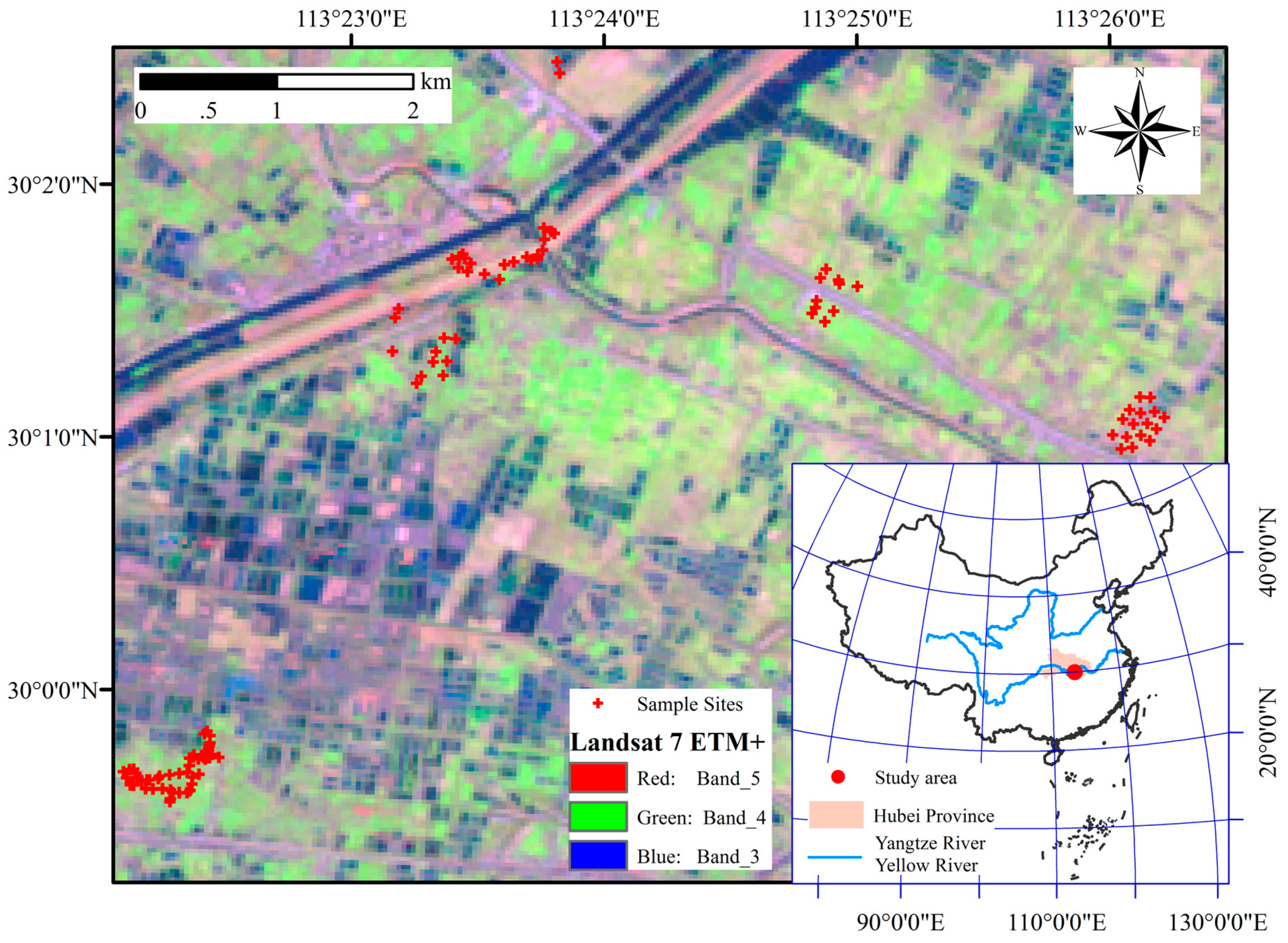
2.1. Study Area

The study area is located in Chahe Town (29°45′18″ N, 113°52′30″ E) in central China (Figure 1). Chahe Town lies on the alluvial plain of Honghu Lake (43,100 ha) with an extensive network of rivers. This plain is one of the major rice-producing areas in China. The plain has a subtropical monsoon climate, with the mean daily temperature of 3.8 °C in winter and 28.9 °C in summer. The mean annual precipitation is 1154 mm, and the rainfall is concentrated in summer (from May to June). The main types of soil are Typical Haplaquept, Dystrochrept, Eutroboralf, and Hapludalf, according to the World Reference Base (WRB) for Soil Resource [36]. The main types of land use are paddy field and irrigated cropland. The region has undergone dramatic changes in land use and land cover, caused by human activities since the 1950s, which have recently raised ecological concerns [37,38].

2.2. Sample Collection

Topsoil samples (0–15 cm; n = 108) were collected in an area of 4340.85 ha in December 2011 (Figure 2). The distance between the sample position was at least 20 meters [39]. All samples were packed in sealed plastic bags, and then transported to the laboratory. Two outliers were identified according to the 3σ criterion, and the remaining 106 samples were used.

2.3. Spectral Measurement and Chemical Analysis

The soil samples were air-dried and ground to pass through a 2-mm sieve. Each sample was divided into two parts: one was for spectral measurement and the other was for chemical analysis. The soil samples were scanned using an ASD FieldSpec^® 3 portable spectro-radiometer (Analytical Spectral Devices Inc., Boulder, CO, USA) with a spectral range of 350–2500 nm. Spectral measurement was conducted in a dark room, and a halogen lamp was used as the source of light at an incidence angle of 45°. The fiber probe was installed 12 cm above the sample surface at a zenith angle of 90°. For each sample, approximately 300 g of soil was placed in a 20-cm-diameter dish with a thickness of about 10 mm. Scans were made 10 times and averaged. SOM was indirectly determined by the potassium dichromate volumetric method in accordance with the Chinese standard (specification of soil test, SL237-1999) [40].

2.4. Spectral Pretreatment

The six most commonly used pretreatments were chosen [41], namely Savitzky–Golay (SG) smoothing [42], first derivative (FD) [43], log(1/R) [44], mean centering (MC) [45], standard normal variate (SNV) [46], and multiplicative scatter correction (MSC) [47].

SG smoothing is a popular filter among smoothing filters to pretreat soil spectra [48]. It is a low-pass filter used to smooth spectra by eliminating high-frequency noise and passing low-frequency signals [49]. This filter fits successive sub-sets (windows) of adjacent data points with a low-degree polynomial through the use of linear least squares. For SG, the size of the window (filter width) is 15 nm and the order of the polynomial is 2 [50]. Derivatives can remove unimportant baseline signals, interferences of background, and spectral overlapping [51]. FD, which is the most commonly used pretreatment for removing baseline offset, was adopted in this study. SG smoothing was carried out before computing the derivatives.

The transformation of reflectance R into log(1/R) will highlight the edges of absorption features and help achieve linearization between the spectra and SOM content [28,52]. Linearization is important for regression models because many modeling methods expect linear responses, which are easier to model than non-linear ones. MC does not reduce multicollinearity in multivariate regression models, but it will improve the numerical stability of some models (e.g., PLSR) [53,54]. MC calculates the mean of a data set and subtracts this from each spectrum:

$${\mathit{x}}_i\left(\mathrm{MC}\right)={\mathit{x}}_i-\overline{\mathit{X}}$$

(1)

where ${\mathit{x}}_i$ is the measured spectrum of sample #i, $\overline{\mathit{X}}$ is the mean spectrum of a data set, and ${\mathit{x}}_i\left(\mathrm{MC}\right)$ is the corrected spectrum.

MSC was first introduced by Martens et al. [55] in 1983 and described in detail by Geladi et al. [47] in 1985. MSC attempts to eliminate or minimize the impact from scattering [28]. MSC hypothesizes that all samples have the same scatter level as the reference spectrum (e.g., the mean spectrum) [56]. Thus, MSC firstly performs a regression of a measured spectrum against the reference spectrum, and then corrects the measured spectrum using the constructed linear regression model. MSC is calculated using Equations (2) and (3).

$${\mathit{x}}_i=\mathbf{1}{a}_i+\overline{\mathit{X}}{b}_i$$

(2)

$${\mathit{x}}_i\left(MSC\right)=({\mathit{x}}_i-\mathbf{1}{a}_i)/b_i$$

(3)

where ${\mathit{x}}_i$ is the measured spectrum of sample #i; $a_i$ and $b_i$ are the intercept and slope, respectively; $\overline{\mathit{X}}$ is the mean spectrum of a data set; ${\mathit{x}}_i\left(MSC\right)$ is the corrected spectrum; and 1 is a vector of ones.

SNV corrects the multiplicative interferences of light scatter and particle size [29], and it has a similar function to MSC [57]. In SNV, each spectrum is transformed by subtracting the spectrum mean and dividing by the spectrum standard deviation [58]. The main difference between the two methods is that SNV is applied to an individual spectrum, whereas MSC uses a reference spectrum [41]. MSC is calculated as follows:

$$\overline{x_i}=\frac{{{\displaystyle \sum }}_{j=1}^m{x}_{ij}}{m}$$

(4)

$$x_{ij}\left(SNV\right)=\frac{x_{ij}-\overline{x_i}}{\sqrt{\frac{{{\displaystyle \sum }}_{j=1}^m{\left(x_{ij}-\overline{x_i}\right)}^2}{m-1}}}$$

(5)

where m is the number of wavelengths, and $x_{ij}$ and $x_{ij}\left(SNV\right)$ are the measured and corrected reflectance of the jth wavelength for the sample #i, respectively.

2.5. Model Calibration

2.5.1. Sample Selection Method

The KS algorithm selects samples sequentially, which are uniformly distributed over the spectral space by choosing samples that maximize the Euclidean distance between each other [35]. The Euclidean distance is based on spectral characteristics and calculated using Equation (6). First, KS selects a pair of samples whose distance between each other is maximum. Second, KS will select a sample individually from the remaining subset. The next sample will be the farthest away from the samples already selected, and that iteration is repeated until the required number of samples is obtained.

$$d\left(m,n\right)=\sqrt{{\displaystyle \sum }_{i=1}^I{\left(x_{mi}-x_{ni}\right)}^2}$$

(6)

where $x_{mi}$ and $x_{ni}$ are the reflectance of samples #m and #n at the ith wavelength, respectively; and I is the number of wavelengths.

2.5.2. Inclusion of Pretreatment in Sample Selection

All 106 samples were sorted in ascending order based on the concentration of SOM, and then 21 samples were chosen at an interval of four samples as the validation set (20% of the total samples). The validation set was used to validate the built models. Such a division strategy is different from sampling for map validation in digital soil mapping, such as purposive sampling and probability sampling [26,37,59,60]. In doing so, we ensured that the validation samples were evenly distributed in the range of the SOM concentration and covered the SOM diversity of expected future samples [44]. Moreover, such a division strategy was commonly adopted in previous studies using vis–NIR spectroscopy to estimate soil properties [27,38,61,62]. The raw spectra of the remaining 85 samples were pretreated by six methods, namely SG, FD, MC, log(1/R), MSC, and SNV. The raw spectra were also used for comparison.

The samples for the calibration set were selected using KS and pretreated spectra. The size of the calibration set was successively increased from 10 samples to 85 samples in increments of one (i.e., 10, 11, …, 85).

2.5.3. PLSR Models

PLSR is a popular technique used to correlate soil spectra with SOM [33,63,64]. Partial least squares regression (PLSR) first projected the spectral data onto a low-dimensional space by maximizing the covariance between the soil spectra and SOM. Multiple regression analysis was then performed in the low-dimensional space. The calibration sets were used to construct the PLSR models. The number of latent variables was determined by the leave-one-out cross-validation (LOOCV). We focused on sample selection; hence, no pretreatment was used in PLSR.

2.6. Performance of Models

The performance of the PLSR models was assessed by a useful statistic, namely the residual predictive deviation (RPD), which was calculated as follows: [65]

$$\mathrm{RPD}=\frac{\mathrm{SD}}{\mathrm{RMSEP}}$$

(7)

where SD is the standard deviation of the reference values, and RMSEP is the root-mean-square error of prediction.

We compared the results of including pretreatment in sample selection with that of not including pretreatment in sample selection, and we calculated $\Delta \mathrm{RPD}$ as follows:

$$\Delta \mathrm{RPD}={\mathrm{RPD}}_{\mathrm{Pretreated}}-{\mathrm{RPD}}_{\mathrm{Raw}}$$

(8)

where ${\mathrm{RPD}}_{\mathrm{Pretreated}}$ is the RPD of the PLSR model when calibration samples were selected using the pretreated spectra, and ${\mathrm{RPD}}_{\mathrm{Raw}}$ is the RPD of the PLSR model when calibration samples were selected using the raw spectra.

3. Results

3.1. Descriptive Statistics of Soil Samples

SOM content varied from 4.06 g kg⁻¹ to 47.34 g kg⁻¹ (

Table 1. Descriptive statistics of 106 soil samples for the calibration and validation sets.

Sample	Number	SOM (g kg−1)						CV 3	Skewness	Kurtosis
		Range 1	Min	Max	Median	Mean	SD 2
Total	106	43.28	4.06	47.34	28.64	27.43	10.59	0.39	−0.19	−1.06
Calibration	85	43.28	4.06	47.34	28.69	27.45	10.67	0.39	−0.20	−1.03
Validation	21	35.75	8.37	44.12	28.59	27.36	10.54	0.39	−0.17	−1.20

¹ Range denotes the difference between the maximum and minimum observations. ² SD denotes standard deviation. ³ CV denotes coefficient of variation. SOM, soil organic matter.

). The coefficient of variation (CV) was 0.39, which indicated that SOM was of medium variability (0.1 < CV < 1.0) [66]. The skewness was −0.19 and was close to zero, thereby implying that the number of samples with low and high SOM contents was similar. The kurtosis was −1.06, which meant that there were less samples around the mean SOM content than in a normal distribution, and the distribution was relatively flat.

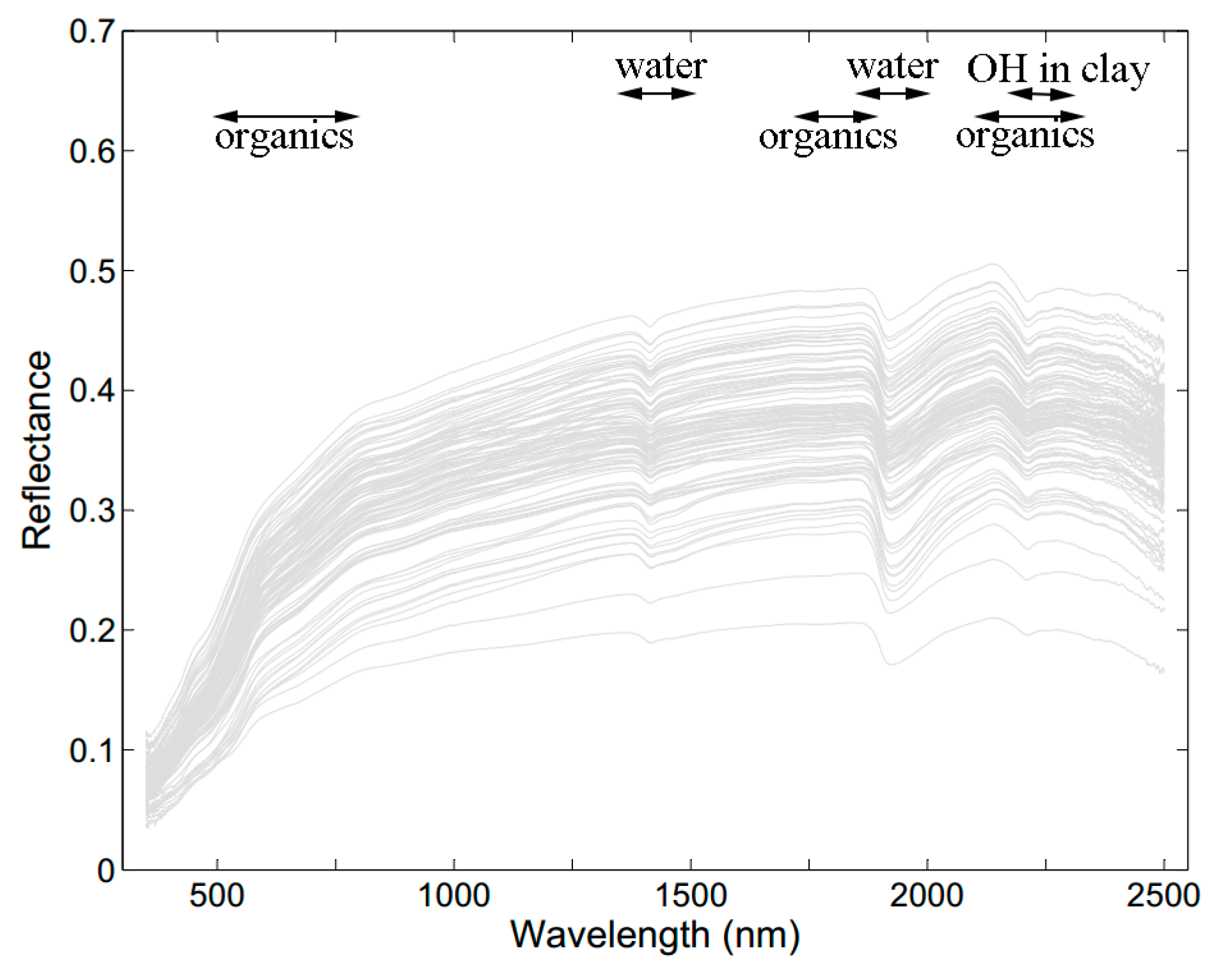
3.2. Soil Spectral Characteristics

The spectral profile showed three prominent absorption peaks at ~1420, 1920, and 2220 nm, which were mainly caused by the hydroxyl group (OH) of free water at 1420 and 1920 nm and the Al–OH lattice structure in clay minerals at 2220 nm (Figure 2) [67]. The shape of the soil spectral reflectance curves was consistent with the results of other studies [14,68].

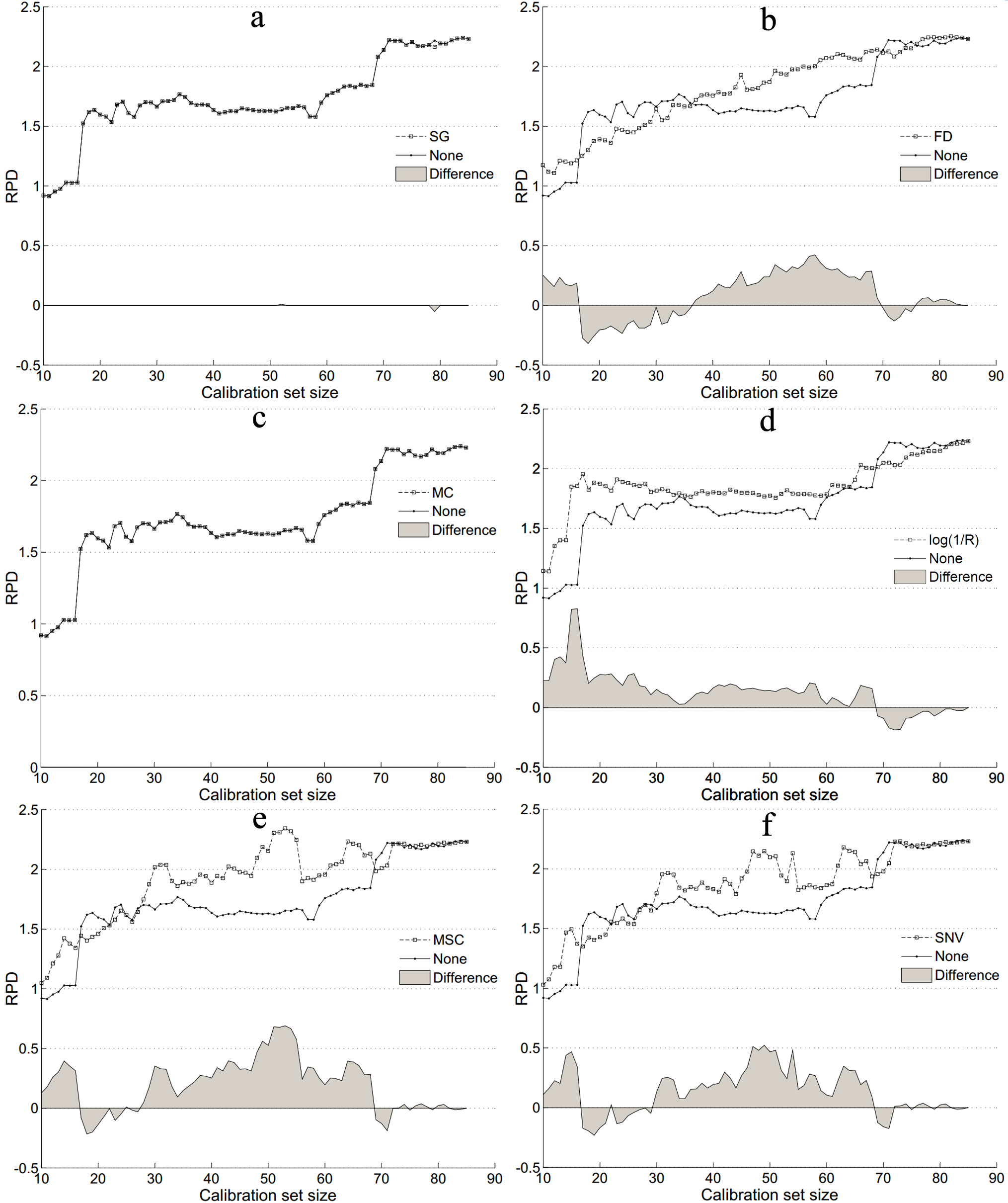
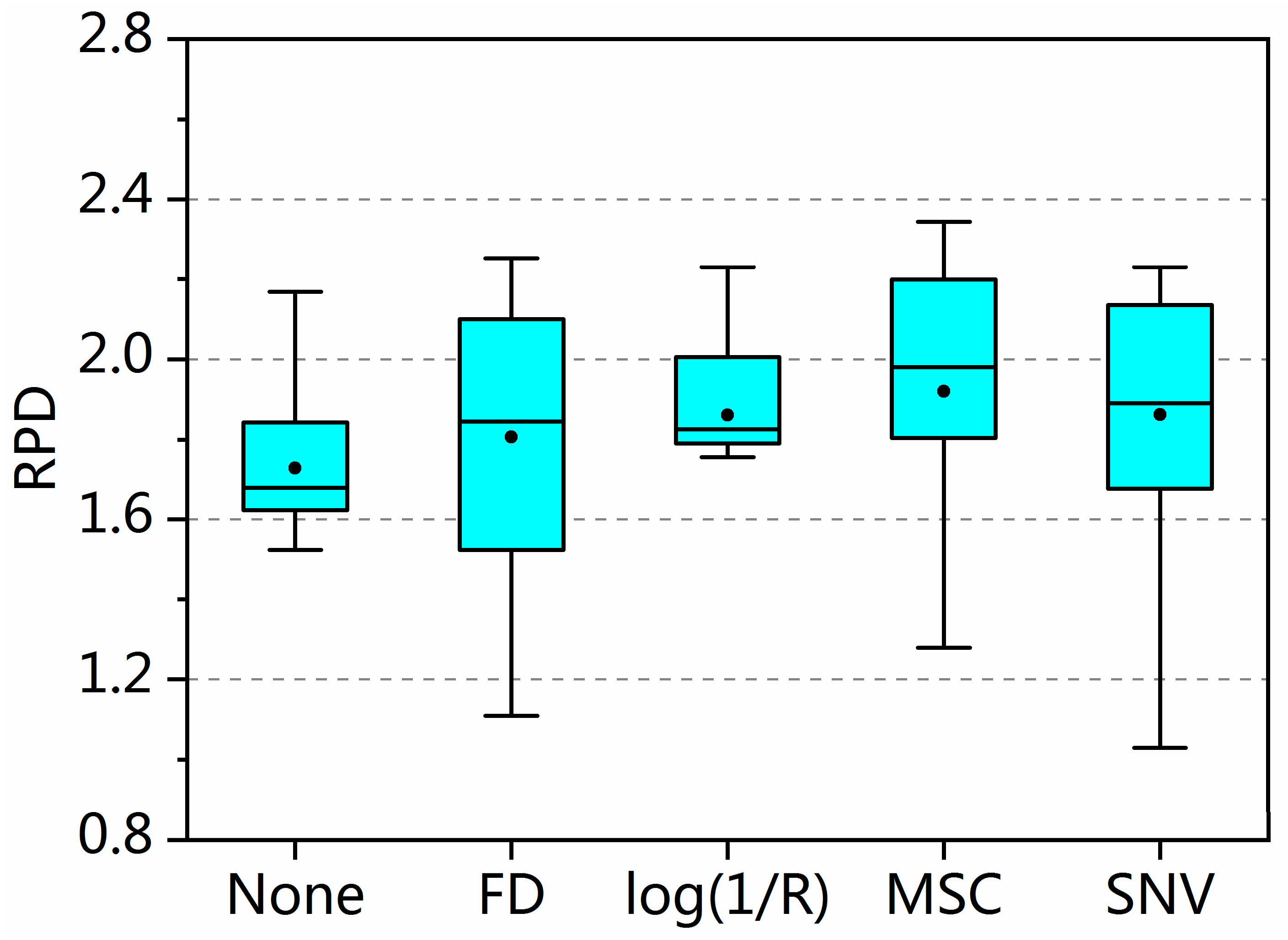
3.3. Accuracy of SOM Prediction after Including Pretreatment in Sample Selection

The control group without applying pretreatment to sample selection was the basis for the following comparison, and its performance is illustrated in Figure 3a. When only a few samples (<16) were selected, the model performed poorly, with an RPD of only ~1.03. The RPD drastically increased up to 1.52 at a calibration set size of 17 samples, remained stable with minor volatility ($\left|\Delta \mathrm{RPD}\right|\le$ 0.24) at a calibration set size <58 samples, increased slowly (from 1.58 to 1.85) at a calibration set size of 58–68 samples, increased sharply (from 1.58 to 2.22) at a calibration set size of 68–71 samples, and then remained stable again.

SG and MC had no impact on sample selection (Figure 3a,c). SG slightly changed the spectra; thus, its effect was nearly negligible. According to Equations (1) and (6), MC will not change the Euclidean distance between samples; hence, it did not affect the sample selection that was based on Euclidean distance.

With the exception of MC and SG, the other four pretreatments affected sample selection differently (Figure 3b,d–f). For FD, the RPD increased linearly from 1.11 to 2.24 when more samples were selected (Figure 3b). FD considerably improved sample selection at calibration set sizes of 37–69 samples.

MSC achieved slightly better results than SNV (Figure 3e,f). MSC extensively helped sample selection at calibration set sizes of 30–68 samples (0.09 $\le \Delta \mathrm{RPD}\le$ 0.69) and obtained the highest RPD (2.34, n = 53). The RPD of a total of 85 calibration samples could only reach 2.22.

log(1/R) improved sample selection at calibration set sizes $\le$68 samples, and the RPD of only 17 samples was as high as 1.96 (Figure 3d). The RPD of the raw spectra was above 1.96 until more than 69 samples were selected. Thus, 17 samples obtained the same results as 69 samples with the aid of spectral pretreatment.

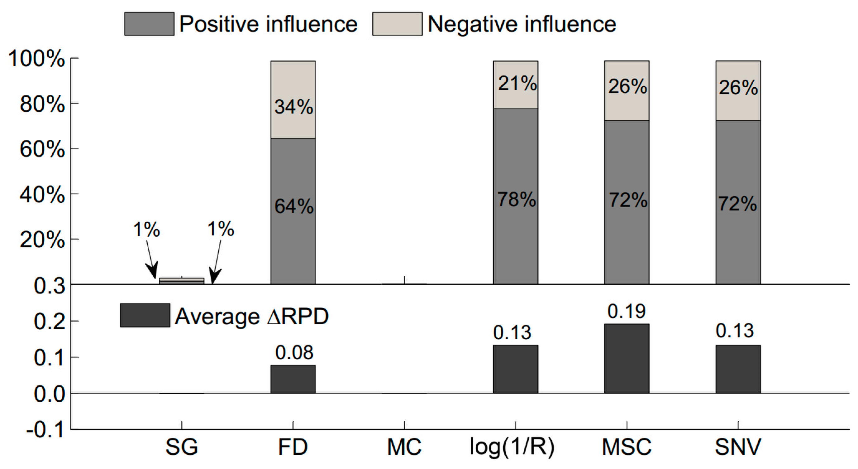
3.4. Proportion of Pretreatment’s Positive or Negative Influence on Sample Selection

The proportion of pretreatment’s positive or negative influence on sample selection is shown in Figure 4. With the exception of SG and MC, the other four pretreatments improved sample selection in over 64 percent of cases, namely FD (64%), log(1/R) (78%), MSC (72%), and SNV (72%). A satisfactory result was also achieved for the average degree of pretreatment’s influence on sample selection (Figure 4). MSC performed best with the highest average $\Delta \mathrm{RPD}$ (0.19), and the improvement was considerable. SNV and log(1/R) obtained the same average $\Delta \mathrm{RPD}$ (0.13). FD slightly influenced sample selection with an average $\Delta \mathrm{RPD}$ of 0.08.

The boxplot of RPD value of the partial squares regression (PLSR) model after including pretreatment in sample selection is shown in Figure 5. Pretreatment improved sample selection in terms of mean, median, third quartile, and third quartile of RPD value. The analysis of variance (ANOVA) showed that log(1/R) and MSC significantly changed sample selection (p < 0.05) (

Table 2. A comparison of different pretreatments in terms of residual predictive deviation (RPD) according to the analysis of variance (ANOVA) with a Games–Howell post-hoc test.

Type of Pretreatment
Variable	N	None	FD	log(1/R)	MSC	SNV
RPD (Mean ± Std. Deviation)	76	1.73 ± 0.33	1.81 ± 0.34 (p = 0.62)	1.86 ± 0.21 * (p = 0.03)	1.92 ± 0.32 * (p = 0.00)	1.86 ± 0.31 (p = 0.08)

Note: FD denotes first derivative, log(1/R) denotes logarithmic function, MSC denotes multiplicative scatter correction, and SNV denotes standard normal variate. An asterisk (*) shows statistically significant differences (p < 0.05) between the mean of RPD after including pretreatment in sample selection.

). Thus, pretreatment’s influence on sample selection was significant and positive in most cases.

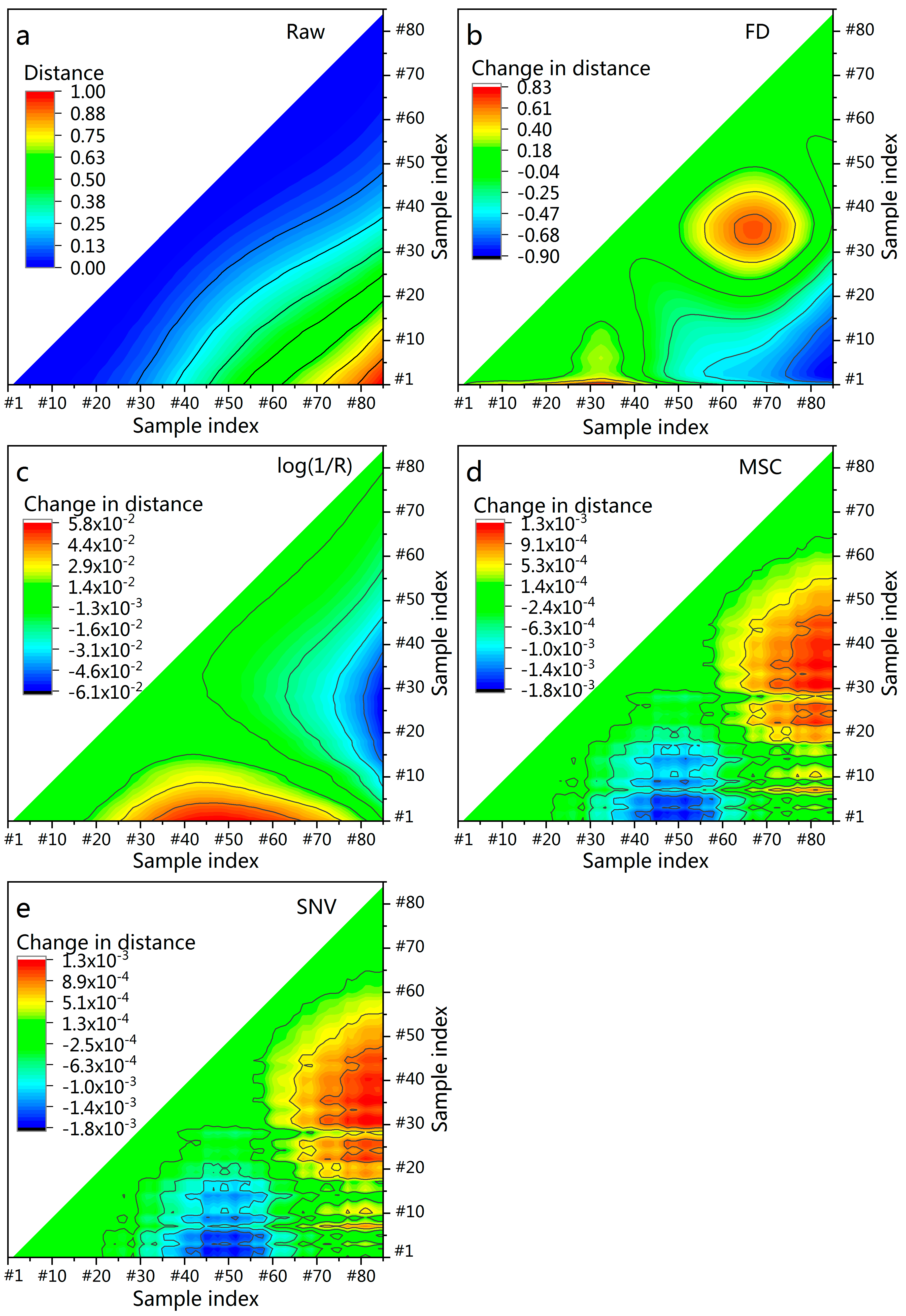
3.5. Euclidean Distance between Samples after Pretreatment

Without pretreatment, the Euclidean distance between samples is shown in Figure 6a. Samples were sorted depending on the SOM concentration. Sample #1 and sample #85 demonstrated the biggest difference in SOM concentration and exhibited the largest spectral distance (bright red). The distance from a sample to itself was zero (dark blue). A “zonal distribution” was observed: the color changed gradually from the bottom right (bright red) to top left (dark blue). In each zone, the difference in SOM concentration of each pair of samples was roughly the same; so is the distance between each pair of samples. The spectral distance gradually increases with SOM concentration difference, resulting in a “zonal distribution”.

After pretreatment, the Euclidean distance between samples changed (Figure 6b–e). SNV had nearly the same effect as MSC: the spectral distance between the pair of samples near the pair (#35, #80) (sample index difference (SID) = 45) was enhanced, whereas the spectral distance near (#50, #5) (SID = 45) was weakened. By contrast, log(1/R) weakened the spectral distance near (#50, #5) (SID = 45), but enhanced the spectral distance near (#30, #80) (SID = 50). FD produced different results from the other pretreatment methods. FD enhanced the spectral distance near (#65, #35) (SID = 30) and (#35, #5) (SID = 30), but it weakened the spectral distance near (#80, #10) (SID = 70).

4. Discussion

4.1. Influence of Pretreatment on Sample Selection

The influence of spectral pretreatment on sample selection varies with the size of the calibration set. For example, log(1/R) considerably improved sample selection at small sample sizes, whereas its influence was slightly weak at large sample sizes (Figure 3d). In addition, when a large proportion of samples was to be selected, spectral pretreatment only slightly influenced sample selection. One reason behind this is that the impact of a newly selected sample on the calibration set weakened with increasing size of the calibration set.

There might be two potential applications. On the one hand, a subset of samples selected by the inclusion of pretreatment could lead to better performance than the total dataset. For example, 58 samples performed better (RPD = 2.34) than the total dataset (RPD = 2.22) with the inclusion of MSC in sample selection. On the other hand, pretreatment may help to reduce the number of calibration samples. For example, 17 samples selected by including the pretreatment of log(1/R) achieved the same model accuracy as 65 samples selected without pretreatments. Isaksson et al. used cluster analysis techniques to select 20 samples that obtained the same model performance as the original 114 samples [69]. Shetty et al. selected 19 samples that represented 118 samples by using Puchwein’s method [13]. In the present study, similar results were obtained by applying pretreatment to sample selection.

Different types of pretreatment can have varied effects on sample selection. MSC performed best, followed by log(1/R), SNV, and FD. By contrast, SG and MC had no impact on sample selection. The reason behind this is that different spectral pretreatments improve the quality of spectra in various ways, such as eliminating the impact from scattering and particle size (SNV and MSC) [29], highlighting the edges of absorption features and achieving linearization (log(1/R)) [28,52], and removing baseline signals and spectral overlapping (FD) [51]. When the pretreated spectra are different, the sample selection method selects different samples. Furthermore, the dataset might be affected by many factors, and only a single pretreatment might not be able to deal with all factors. Therefore, the optimal pretreatment depends on the dataset used, and a combination of multiple pretreatments might be more useful for sample selection, which requires further study.

4.2. How Pretreatment Affects Sample Selection

Pretreatment affects sample selection by changing the spectral distance (the Euclidean distance) between samples, and the change might be an enhancement or weakening. For log(1/R), MSC, and SNV, the change is near (mean SOM concentration, low SOM concentration) and (mean SOM concentration, high SOM concentration). Thus, the change near the mean SOM concentration may facilitate sample selection. The reason behind this is that the sample closest to the mean is deemed to be the most representative [33,70]. However, FD changed the distance near (high SOM concentration, low SOM concentration) and its influence was weaker than that of the other three pretreatments.

The change in distance affects the process of selecting samples. Figure 7 illustrates an example of how KS selects 14 samples. After pretreatment with log(1/R), more representative samples were selected, and the RPD increased from 1.03 to 1.40. The major differences in sample selection between raw and pretreated spectra were low SOC (Sample #10), mean SOC (Sample #35 and #55), and high SOC (Sample #76 and #80). This finding was in line with our previous results of distance change. Another difference is that the intervals between adjacent samples become reasonable. For example, samples #42 and #61 were selected without pretreatment, and the interval was large. However, after pretreatment, samples #40 and #55 were selected, and the interval decreased. Thus, pretreatment in sample selection could determine a subset of samples that spans the same space, but is more evenly distributed in the space [71]. From the perspective of regression, a flat distribution of data is more favorable than a normal distribution [13].

Pretreatment is usually used in multivariate regression models (e.g., PLSR). In the present study, pretreatment was used in sample selection. In multivariate regression analysis, the aim of pretreatment is to improve model performance. Pretreatment works by linearizing the response of a variable and removing noise [72]. However, when selecting samples, representative samples should be selected. Pretreatment works by changing the differences or similarities between samples [56,73]. Thus, the effects of pretreatments on multivariate regression analysis and sample selection differed. This difference was verified by the results of

Table 3. Cross-validation of applying pretreatments to multivariate regression analysis for estimating soil organic matter (SOM).

Pretreatment	${\mathbf{R}}_{\mathbf{c}\mathbf{v}}^{\mathbf{2}}$	$\mathbf{R}\mathbf{M}\mathbf{S}{\mathbf{E}}_{\mathbf{c}\mathbf{v}}\mathbf{\left(}\mathbf{g}\mathbf{·}\mathbf{k}{\mathbf{g}}^{\mathbf{-}\mathbf{1}}\mathbf{\right)}$	RPD	$\mathbf{\Delta }\mathbf{R}\mathbf{P}\mathbf{D}$
None	0.72	5.71	1.87	-
SG	0.72	5.71	1.87	−0.00
FD	0.80	4.74	2.25	0.38
MC	0.67	6.09	1.75	−0.12
log(1/R)	0.59	6.82	1.56	−0.31
MSC	0.66	6.20	1.72	−0.15
SNV	0.74	5.47	1.95	0.08

Note: SG denotes Savitzky–Golay smoothing, FD denotes first derivative, MC denotes mean centering, log(1/R) denotes logarithmic function, MSC denotes multiplicative scatter correction, SNV denotes standard normal variate, ${\mathrm{RMSE}}_{\mathrm{cv}}$ denotes the root-mean-square error of cross-validation, ${\mathrm{R}}_{\mathrm{cv}}^2$ denotes the coefficient of determination for cross-validation, RPD denotes residual predictive deviation, and $\Delta \mathrm{RPD}$ denotes changed RPD.

and Figure 4. In addition, if a pretreatment was useful in multivariate regression analysis, it was not necessarily useful in sample selection. For example, log(1/R) considerably improved sample selection, but it worsened the PLSR model.

The soil samples we used were arid-dried, ground, and sieved. During in-situ application, field spectra were affected by environmental factors, such as soil water content and soil surface roughness [74]. The removal of effects of water from field spectra could increase the performance of multivariate regression models [25,75]. The use of spectral pretreatment to remove the effects of environmental factors on field spectra might also help sample selection methods, which requires further study.

5. Conclusions

This present study included spectral pretreatment in a sample selection strategy to select calibration samples for the SOM estimation using vis–NIR spectroscopy. From our results, we draw the following conclusions: (i) the inclusion of spectral pretreatment in sample selection can select more representative samples and improve the subsequent performance of SOC estimation; and (ii) the degree of the influence of pretreatment on sample selection can differ depending on the size of the calibration set and the type of pretreatment.

Despite our success in including pretreatment in sample selection to improve SOM estimation using vis-NIR spectroscopy, sample selection and SOM estimation can still be improved. Future research should be focused on other sample selection methods, increasing the sampling density, field spectra, and the inclusion of multiple pretreatments in sample selection. Our study is based on local samples, but our strategy might also be useful at a national scale.

References

1. Lal, R. Soil carbon sequestration impacts on global climate change and food security. Science 2004, 304, 1623–1627. [Google Scholar] [CrossRef] [PubMed]
2. Schmidt, M.W.; Torn, M.S.; Abiven, S.; Dittmar, T.; Guggenberger, G.; Janssens, I.A.; Kleber, M.; Kögel-Knabner, I.; Lehmann, J.; Manning, D.A. Persistence of soil organic matter as an ecosystem property. Nature 2011, 478, 49–56. [Google Scholar] [CrossRef] [PubMed] [Green Version]
3. Lehmann, J.; Kleber, M. The contentious nature of soil organic matter. Nature 2015, 528, 60–68. [Google Scholar] [CrossRef] [PubMed]
4. Walkley, A.; Black, I.A. An examination of the Degtjareff method for determining soil organic matter, and a proposed modification of the chromic acid titration method. Soil Sci. 1934, 37, 29–38. [Google Scholar] [CrossRef]
5. Nelson, D.; Sommers, L.E. Total carbon, organic carbon, and organic matter. In Methods of Soil Analysis. Part 2. Chemical and Microbiological Properties; American Society of Agronomy Inc.: Madison, WI, USA, 1982; pp. 539–579. [Google Scholar]
6. Shi, Z.; Ji, W.; Viscarra Rossel, R.A.; Chen, S.; Zhou, Y. Prediction of soil organic matter using a spatially constrained local partial least squares regression and the Chinese vis–NIR spectral library. Eur. J. Soil Sci. 2015, 66, 679–687. [Google Scholar] [CrossRef]
7. Bellon-Maurel, V.; McBratney, A. Near-infrared (NIR) and mid-infrared (MIR) spectroscopic techniques for assessing the amount of carbon stock in soils—Critical review and research perspectives. Soil Biol. Biochem. 2011, 43, 1398–1410. [Google Scholar] [CrossRef]
8. Ben-Dor, E.; Banin, A. Near infrared analysis (NIRA) as a method to simultaneously evaluate spectral featureless constituents in soils. Soil Sci. 1995, 159, 259–270. [Google Scholar] [CrossRef]
9. Guerrero, C.; Zornoza, R.; Gómez, I.; Mataix-Beneyto, J. Spiking of NIR regional models using samples from target sites: Effect of model size on prediction accuracy. Geoderma 2010, 158, 66–77. [Google Scholar] [CrossRef]
10. Fidencio, P.H.; Poppi, R.J.; de Andrade, J.C. Determination of organic matter in soils using radial basis function networks and near infrared spectroscopy. Anal. Chim. Acta 2002, 453, 125–134. [Google Scholar] [CrossRef]
11. Ge, Y.; Morgan, C.; Thomasson, J.; Waiser, T. A new perspective to near-infrared reflectance spectroscopy: A wavelet approach. Trans. ASABE 2007, 50, 303–311. [Google Scholar] [CrossRef]
12. Gholizadeh, A.; Borůvka, L.; Saberioon, M.; Vašát, R. Visible, near-infrared, and mid-infrared spectroscopy applications for soil assessment with emphasis on soil organic matter content and quality: State-of-the-art and key issues. Appl. Spectrosc. 2013, 67, 1349–1362. [Google Scholar] [CrossRef] [PubMed]
13. Shetty, N.; Rinnan, Å.; Gislum, R. Selection of representative calibration sample sets for near-infrared reflectance spectroscopy to predict nitrogen concentration in grasses. Chemom. Intell. Lab. Syst. 2012, 111, 59–65. [Google Scholar] [CrossRef]
14. Ramirez-Lopez, L.; Schmidt, K.; Behrens, T.; van Wesemael, B.; Dematte, J.A.; Scholten, T. Sampling optimal calibration sets in soil infrared spectroscopy. Geoderma 2014, 226, 140–150. [Google Scholar] [CrossRef]
15. Kuang, B.; Mouazen, A.M. Influence of the number of samples on prediction error of visible and near infrared spectroscopy of selected soil properties at the farm scale. Eur. J. Soil Sci. 2012, 63, 421–429. [Google Scholar] [CrossRef] [Green Version]
16. Kennard, R.W.; Stone, L.A. Computer aided design of experiments. Technometrics 1969, 11, 137–148. [Google Scholar] [CrossRef]
17. Massart, D.L.; Vandeginste, B.G.; Buydens, L.; Lewi, P.; Smeyers-Verbeke, J.; Jong, S.D. Handbook of Chemometrics and Qualimetrics: Part A; Elsevier Science Inc.: Amsterdam, The Netherlands, 1997. [Google Scholar]
18. Galvao, R.K.H.; Araujo, M.C.U.; Jose, G.E.; Pontes, M.J.C.; Silva, E.C.; Saldanha, T.C.B. A method for calibration and validation subset partitioning. Talanta 2005, 67, 736–740. [Google Scholar] [CrossRef] [PubMed]
19. Udelhoven, T.; Emmerling, C.; Jarmer, T. Quantitative analysis of soil chemical properties with diffuse reflectance spectrometry and partial least-square regression: A feasibility study. Plant Soil 2003, 251, 319–329. [Google Scholar] [CrossRef]
20. Stevens, A.; Udelhoven, T.; Denis, A.; Tychon, B.; Lioy, R.; Hoffmann, L.; Van Wesemael, B. Measuring soil organic carbon in croplands at regional scale using airborne imaging spectroscopy. Geoderma 2010, 158, 32–45. [Google Scholar] [CrossRef] [Green Version]
21. Nocita, M.; Stevens, A.; Toth, G.; Panagos, P.; van Wesemael, B.; Montanarella, L. Prediction of soil organic carbon content by diffuse reflectance spectroscopy using a local partial least square regression approach. Soil Biol. Biochem. 2014, 68, 337–347. [Google Scholar] [CrossRef]
22. Peng, Y.; Knadel, M.; Gislum, R.; Deng, F.; Norgaard, T.; de Jonge, L.W.; Moldrup, P.; Greve, M.H. Predicting soil organic carbon at field scale using a national soil spectral library. J. Near Infrared Spectrosc. 2013, 21, 213–222. [Google Scholar] [CrossRef]
23. Vasques, G.M.; Grunwald, S.; Harris, W.G. Spectroscopic models of soil organic carbon in Florida, USA. J. Environ. Q. 2010, 39, 923–934. [Google Scholar] [CrossRef] [PubMed]
24. Wienhold, B.J.; Power, J.F.; Doran, J.W. Agricultural accomplishments and impending concerns. Soil Sci. 2000, 165, 13–30. [Google Scholar] [CrossRef]
25. Ji, W.J.; Li, S.; Chen, S.C.; Shi, Z.; Viscarra Rossel, R.A.; Mouazen, A.M. Prediction of soil attributes using the Chinese soil spectral library and standardized spectra recorded at field conditions. Soil Tillage Res. 2016, 155, 492–500. [Google Scholar] [CrossRef]
26. De Gruijter, J.; Brus, D.J.; Bierkens, M.F.; Knotters, M. Sampling for Natural Resource Monitoring; Springer Science & Business Media: Berlin, Germany, 2006. [Google Scholar]
27. Liu, Y.; Shi, Z.; Zhang, G.; Chen, Y.; Li, S.; Hong, Y.; Shi, T.; Wang, J.; Liu, Y. Application of Spectrally Derived Soil Type as Ancillary Data to Improve the Estimation of Soil Organic Carbon by Using the Chinese Soil Vis-NIR Spectral Library. Remote Sens. 2018, 10, 1747. [Google Scholar] [CrossRef]
28. Shi, T.; Chen, Y.; Liu, Y.; Wu, G. Visible and near-infrared reflectance spectroscopy-An alternative for monitoring soil contamination by heavy metals. J. Hazard. Mater. 2014, 265, 166–176. [Google Scholar] [CrossRef] [PubMed]
29. Gholizadeh, A.; Borůvka, L.; Saberioon, M.M.; Kozak, J.; Vasat, R.; Nemecek, K. Comparing different data preprocessing methods for monitoring soil heavy metals based on soil spectral features. Soil Water Res. 2015, 10, 218–227. [Google Scholar] [CrossRef]
30. Gholizadeh, A.; Saberioon, M.; Carmon, N.; Borůvka, L.; Ben-Dor, E. Examining the Performance of PARACUDA-II Data-Mining Engine versus Selected Techniques to Model Soil Carbon from Reflectance Spectra. Remote Sens. 2018, 10, 1172. [Google Scholar] [CrossRef]
31. Gholizadeh, A.; Carmon, N.; Klement, A.; Ben-Dor, E.; Borůvka, L. Agricultural Soil Spectral Response and Properties Assessment: Effects of Measurement Protocol and Data Mining Technique. Remote Sens. 2017, 9, 1078. [Google Scholar] [CrossRef]
32. Debaene, G.; Niedźwiecki, J.; Pecio, A.; Żurek, A. Effect of the number of calibration samples on the prediction of several soil properties at the farm-scale. Geoderma 2014, 214, 114–125. [Google Scholar] [CrossRef]
33. Li, Z.; Liu, J.; Shan, P.; Peng, S.; Lv, J.; Ma, Z. Strategy for constructing calibration sets based on a derivative spectra information space consensus. Chemom. Intell. Lab. Syst. 2016, 156, 7–13. [Google Scholar] [CrossRef]
34. Stevens, A.; Nocita, M.; Tóth, G.; Montanarella, L.; van Wesemael, B. Prediction of soil organic carbon at the European scale by visible and near infrared reflectance spectroscopy. PLoS ONE 2013, 8, e66409. [Google Scholar] [CrossRef] [PubMed]
35. Cao, N. Calibration Optimization and Efficiency in Near Infrared Spectroscopy. Ph.D. Thesis, Iowa State University, Ames, IA, USA, 2013. [Google Scholar]
36. Liu, Y.; Guo, L.; Jiang, Q.; Zhang, H.T.; Chen, Y. Comparing geospatial techniques to predict SOC stocks. Soil Tillage Res. 2015, 148, 46–58. [Google Scholar] [CrossRef]
37. Knotters, M.; Brus, D. Purposive versus random sampling for map validation: A case study on ecotope maps of floodplains in the Netherlands. Ecohydrology 2013, 6, 425–434. [Google Scholar] [CrossRef]
38. Liu, Y.; Jiang, Q.; Fei, T.; Wang, J.; Shi, T.; Guo, K.; Li, X.; Chen, Y. Transferability of a Visible and Near-Infrared Model for Soil Organic Matter Estimation in Riparian Landscapes. Remote Sens. 2014, 6, 4305–4322. [Google Scholar] [CrossRef] [Green Version]
39. Liu, Y.L.; Jiang, Q.H.; Shi, T.Z.; Fei, T.; Wang, J.J.; Liu, G.L.; Chen, Y.Y. Prediction of total nitrogen in cropland soil at different levels of soil moisture with Vis/NIR spectroscopy. Acta Agric. Scand. Sect. B Soil Plant Sci. 2014, 64, 267–281. [Google Scholar] [CrossRef]
40. Zhang, J.; Xu, Z. Dye tracer infiltration technique to investigate macropore flow paths in Maka Mountain, Yunnan Province, China. J. Cent. South Univ. 2016, 23, 2101–2109. [Google Scholar] [CrossRef]
41. Rinnan, A.; van den Berg, F.; Engelsen, S.B. Review of the most common pre-processing techniques for near-infrared spectra. Trac-Trends Anal. Chem. 2009, 28, 1201–1222. [Google Scholar] [CrossRef]
42. Steinier, J.; Termonia, Y.; Deltour, J. Smoothing and differentiation of data by simplified least square procedure. Anal. Chem. 1972, 44, 1906–1909. [Google Scholar] [CrossRef]
43. Naes, T.; Martens, H. Multivariate Calibration; Norwegian Food Research Institute: Oslovegen, Norway, 1989. [Google Scholar]
44. Stenberg, B.; Viscarra Rossel, R.A.; Mouazen, A.M.; Wetterlind, J. Chapter five-visible and near infrared spectroscopy in soil science. Adv. Agron. 2010, 107, 163–215. [Google Scholar]
45. Rossel Viscarra, R.A. ParLeS: Software for chemometric analysis of spectroscopic data. Chemom. Intell. Lab. Syst. 2008, 90, 72–83. [Google Scholar] [CrossRef]
46. Barnes, R.; Dhanoa, M.; Lister, S.J. Standard normal variate transformation and de-trending of near-infrared diffuse reflectance spectra. Appl. Spectrosc. 1989, 43, 772–777. [Google Scholar] [CrossRef]
47. Geladi, P.; Macdougall, D.; Martens, H. Linearization and Scatter-Correction for Near-Infrared Reflectance Spectra of Meat. ApSpe 1985, 39, 491–500. [Google Scholar] [CrossRef]
48. Askari, M.S.; Cui, J.; O’Rourke, S.M.; Holden, N.M. Evaluation of soil structural quality using VIS–NIR spectra. Soil Tillage Res. 2015, 146, 108–117. [Google Scholar] [CrossRef]
49. Hook, J. Smoothing non-smooth systems with low-pass filters. Phys. D Nonlinear Phenom. 2014, 269, 76–85. [Google Scholar] [CrossRef] [Green Version]
50. Delwiche, S.R. A graphical method to evaluate spectral preprocessing in multivariate regression calibrations: Example with Savitzky-Golay filters and partial least squares regression. Appl. Spectrosc. 2010, 64, 73–82. [Google Scholar] [CrossRef]
51. Shetty, N.; Gislum, R. Quantification of fructan concentration in grasses using NIR spectroscopy and PLSR. Field Crops Res. 2011, 120, 31–37. [Google Scholar] [CrossRef]
52. West, J.B.; Bowen, G.J.; Dawson, T.E.; Tu, K.P. Isoscapes: Understanding Movement, Pattern, and Process on Earth through Isotope Mapping; Springer: Heidelberg, Germany, 2009; Volume 3, p. 76. [Google Scholar]
53. Kuhn, M.; Johnson, K. Data pre-processing. In Applied Predictive Modeling; Springer: New York, NY, USA, 2013; pp. 59. [Google Scholar]
54. Echambadi, R.; Hess, J.D. Mean-centering does not alleviate collinearity problems in moderated multiple regression models. Mark. Sci. 2007, 26, 438–445. [Google Scholar] [CrossRef]
55. Martens, H.; Jensen, S.; Geladi, P. Multivariate linearity transformation for near-infrared reflectance spectrometry. In Proceedings of the Nordic Symposium on Applied Statistics; Stokkand Forlag Publishers: Stavanger, Norway, 1983; pp. 205–234. [Google Scholar]
56. Rozenstein, O.; Paz-Kagan, T.; Salbach, C.; Karnieli, A. Comparing the Effect of Preprocessing Transformations on Methods of Land-Use Classification Derived From Spectral Soil Measurements. IEEE J. Sel. Top. Appl. Earth Obs. Remote Sens. 2015, 8, 2393–2404. [Google Scholar] [CrossRef]
57. Dhanoa, M.; Lister, S.; Sanderson, R.; Barnes, R. The link between multiplicative scatter correction (MSC) and standard normal variate (SNV) transformations of NIR spectra. J. Near Infrared Spectrosc. 1994, 2, 43–47. [Google Scholar] [CrossRef]
58. Candolfi, A.; De Maesschalck, R.; Jouan-Rimbaud, D.; Hailey, P.; Massart, D. The influence of data pre-processing in the pattern recognition of excipients near-infrared spectra. J. Pharm. Biomed. Anal. 1999, 21, 115–132. [Google Scholar] [CrossRef]
59. Brus, D.J.; Kempen, B.; Heuvelink, G.B.M. Sampling for validation of digital soil maps. Eur. J. Soil Sci. 2011, 62, 394–407. [Google Scholar] [CrossRef]
60. Rossiter, D. Assessing the thematic accuracy of area-class soil maps; Soil Science Division, ITC: Enschede, The Netherlands, 2001; waiting publication. [Google Scholar]
61. Li, S.; Shi, Z.; Chen, S.; Ji, W.; Zhou, L.; Yu, W.; Webster, R. In situ measurements of organic carbon in soil profiles using vis-NIR spectroscopy on the Qinghai–Tibet plateau. Environ. Sci. Technol. 2015, 49, 4980–4987. [Google Scholar] [CrossRef] [PubMed]
62. Hong, Y.; Yu, L.; Chen, Y.; Liu, Y.; Liu, Y.; Liu, Y.; Cheng, H. Prediction of Soil Organic Matter by VIS–NIR Spectroscopy Using Normalized Soil Moisture Index as a Proxy of Soil Moisture. Remote Sens. 2017, 10, 28. [Google Scholar] [CrossRef]
63. Goodarzi, M.; Sharma, S.; Ramon, H.; Saeys, W. Multivariate calibration of NIR spectroscopic sensors for continuous glucose monitoring. TrAC Trends Anal. Chem. 2015, 67, 147–158. [Google Scholar] [CrossRef] [Green Version]
64. Della Riccia Giacomo, D.Z.S. A multivariate regression model for detection of fumonisins content in maize from near infrared spectra. Food Chem. 2013, 141, 4289–4294. [Google Scholar] [CrossRef] [PubMed]
65. Williams, P.C. Variable affecting near infrared reflectance spectroscopic analysis. Near-Infrared Technol. Agric. Food Ind. 1987, 143–167. [Google Scholar]
66. Yang, Q.Y.; Jiang, Z.C.; Li, W.J.; Li, H. Prediction of soil organic matter in peak-cluster depression region using kriging and terrain indices. Soil Tillage Res. 2014, 144, 126–132. [Google Scholar] [CrossRef]
67. Summers, D.; Lewis, M.; Ostendorf, B.; Chittleborough, D. Visible near-infrared reflectance spectroscopy as a predictive indicator of soil properties. Ecol. Indic. 2011, 11, 123–131. [Google Scholar] [CrossRef]
68. Li, D.; Chen, X.; Peng, Z.; Chen, S.; Chen, W.; Han, L.; Li, Y. Prediction of soil organic matter content in a litchi orchard of South China using spectral indices. Soil Tillage Res. 2012, 123, 78–86. [Google Scholar] [CrossRef] [Green Version]
69. Isaksson, T.; Næs, T. Selection of samples for calibration in near-infrared spectroscopy. Part II: Selection based on spectral measurements. Appl. Spectrosc. 1990, 44, 1152–1158. [Google Scholar] [CrossRef]
70. Walczak, B.; Massart, D.L. Application of Radial Basis Functions—Partial Least Squares to non-linear pattern recognition problems: Diagnosis of process faults. Anal. Chim. Acta 1996, 331, 187–193. [Google Scholar] [CrossRef]
71. Bakeev, K.A. Process Analytical technology: Spectroscopic Tools and Implementation Strategies for the Chemical and Pharmaceutical Industries; John Wiley & Sons: New York, NY, USA, 2010. [Google Scholar]
72. Gras, J.-P.; Barthès, B.G.; Mahaut, B.; Trupin, S. Best practices for obtaining and processing field visible and near infrared (VNIR) spectra of topsoils. Geoderma 2014, 214, 126–134. [Google Scholar] [CrossRef]
73. Schwartz, G.; Ben-Dor, E.; Eshel, G. Quantitative assessment of hydrocarbon contamination in soil using reflectance spectroscopy: A "multipath" approach. Appl. Spectrosc. 2013, 67, 1323. [Google Scholar] [CrossRef] [PubMed]
74. Ji, W.; Rossel Viscarra, R.A.; Shi, Z. Accounting for the effects of water and the environment on proximally sensed vis-NIR soil spectra and their calibrations. Eur. J. Soil Sci. 2015, 66, 555–565. [Google Scholar] [CrossRef]
75. Ge, Y.F.; Morgan, C.L.S.; Ackerson, J.P. VisNIR spectra of dried ground soils predict properties of soils scanned moist and intact. Geoderma 2014, 221, 61–69. [Google Scholar] [CrossRef]
Figure 1. Maps that show the location of the sampled region, the positions of the sampling sites, and the landscapes, as indicated by a Landsat 7 enhanced thematic mapper plus (ETM+) scan line corrector off (SLC-off) image with a composition of bands 4 (red), 3 (green), and 2 (blue).
Remotesensing 11 00450 g001
Figure 2. The spectral reflectance of soil samples (n = 106). The principal positions of spectral absorption by organics and water are highlighted.
Remotesensing 11 00450 g002
Figure 3. The results of pretreatment’s (hollow square) influence on sample selection. None (black circle) denotes the result of sample selection without pretreatment. SG denotes Savitzky–Golay smoothing (a). FD denotes first derivative (b). MC denotes mean centering (c). log(1/R) denotes logarithmic function (d). MSC denotes multiplicative scatter correction (e). SNV denotes standard normal variate (f). RPD denotes residual predictive deviation.
Remotesensing 11 00450 g003
Figure 4. The results of the proportion of calibration sets when pretreatment influenced sample selection positively (dark gray bar) or negatively (light gray bar) and the average Δ RPD (black bar). SG denotes Savitzky–Golay smoothing. FD denotes first derivative. MC denotes mean centering. log(1/R) denotes logarithmic function. MSC denotes multiplicative scatter correction. SNV denotes standard normal variate.
Remotesensing 11 00450 g004
Figure 5. A boxplot of the RPD of the partial least squares regression (PLSR) model after including pretreatment in sample selection. FD denotes first derivative. log(1/R) denotes logarithmic function. MSC denotes multiplicative scatter correction. SNV denotes standard normal variate.
Remotesensing 11 00450 g005
Figure 6. The Euclidean distance among samples of raw spectra (a) and the change in Euclidean distance after the spectra were pretreated by first derivative (FD) (b), logarithmic function (log(1/R)) (c), multiplicative scatter correction (MSC) (d), and standard normal variate (SNV) (e). All the calibration samples are sorted in ascending order according to SOM content and then numbered #1, #2, …, #85.
Remotesensing 11 00450 g006
Figure 7. A subset of 14 samples selected based on raw and pretreated spectra. The gray ellipse shows the major difference in sample selection between raw and pretreated spectra.
Remotesensing 11 00450 g007