Glacier Facies Mapping Using a Machine-Learning Algorithm: The Parlung Zangbo Basin Case Study


1
State Key Laboratory of Remote Sensing Science, Institute of Remote Sensing and Digital Earth, Chinese Academy of Sciences, Beijing 100101, China
2
University of Chinese Academy of Sciences, Beijing 100049, China
3
Department of Geoscience and Remote Sensing, Delft University of Technology, Stevinweg 1, 2628 CN Delft, The Netherlands
*
Author to whom correspondence should be addressed.
Remote Sens. 2019, 11(4), 452; https://0-doi-org.brum.beds.ac.uk/10.3390/rs11040452
Submission received: 21 December 2018
/
Revised: 11 February 2019
/
Accepted: 18 February 2019
/
Published: 22 February 2019
(This article belongs to the Special Issue Remote Sensing of Glaciers at Global and Regional Scales)
Abstract
:Glaciers in the Tibetan Plateau are an important indicator of climate change. Automatic glacier facies mapping utilizing remote sensing data is challenging due to the spectral similarity of supraglacial debris and the adjacent bedrock. Most of the available glacier datasets do not provide the boundary of clean ice and debris-covered glacier facies, while debris-covered glacier facies play a key role in mass balance research. The aim of this study was to develop an automatic algorithm to distinguish ice cover types based on multi-temporal satellite data, and the algorithm was implemented in a subregion of the Parlung Zangbo basin in the southeastern Tibetan Plateau. The classification method was built upon an automated machine learning approach: Random Forest in combination with the analysis of topographic and textural features based on Landsat-8 imagery and multiple digital elevation model (DEM) data. Very high spatial resolution Gao Fen-1 (GF-1) Panchromatic and Multi-Spectral (PMS) imagery was used to select training samples and validate the classification results. In this study, all of the land cover types were classified with overall good performance using the proposed method. The results indicated that fully debris-covered glaciers accounted for approximately 20.7% of the total glacier area in this region and were mainly distributed at elevations between 4600 m and 4800 m above sea level (a.s.l.). Additionally, an analysis of the results clearly revealed that the proportion of small size glaciers (<1 km2) were 88.3% distributed at lower elevations compared to larger size glaciers (≥1 km2). In addition, the majority of glaciers (both in terms of glacier number and area) were characterized by a mean slope ranging between 20° and 30°, and 42.1% of glaciers had a northeast and north orientation in the Parlung Zangbo basin.

1. Introduction
Glaciers in the Tibetan Plateau are sensitive and exhibit an immediate response to climate forcing; hence, they are important climate change indicators [1,2,3]. It is, therefore, meaningful to observe and understand the dynamics and response of glaciers to changes in climatic conditions. Traditional methods of mapping glacier surface types are based on field surveys and analyzing topographic maps, which are very time-consuming and not feasible in inaccessible regions [4]. Nowadays, a vast amount of satellite data allows us to monitor the glaciers over large areas and in high altitude mountainous regions in a cheaper and efficient way. Remote sensing data usually can provide measurements of glacier coverage, glacier number, time span, and other glacier properties [5].
In the past few decades, much work has been accomplished to map the extent of clean glacial ice and to quantify changes over time using satellite image data [6]. Methods applied range from visual interpretation [7] to segmentation of band ratio or spectral indices (e.g., the Normalized Difference Snow Index) images [8] and different unsupervised (e.g., the Iterative Self Organizing Data Analysis Techniques Algorithm, ISODATA) [9] and supervised (e.g., the Maximum Likelihood algorithm) classification [10] and decision tree methods [5,11]. For extracting debris-covered glaciers using multispectral imagery, fully manual onscreen digitizing is widely considered to be a common classification approach [12]. However, the accuracy of results using manual approaches depends greatly on the researcher’s experience. Due to the laborious work of manual delineation, many researchers have further proposed semi-automated methods to extract the debris-covered glacial surface [13,14]. The use of Unmanned Aerial Vehicles (UAVs) and terrestrial remote sensing techniques offers new ways to monitor the debris-covered glaciers on a detailed spatial scale [15,16].
Nevertheless, the spatial heterogeneity of the glacier surface still hampers the identification of glaciers and increases the difficulty of observing and understanding glacier changes. Automated mapping of glaciers based on remotely sensed multispectral data is often hindered by orographic clouds, highly variable snow conditions, and the spectral similarity of supraglacial debris with the adjacent bedrock [6]. However, supraglacial debris can remain stable on gentle slopes [13]. Field measurements and energy balance modeling results indicate that the surface temperatures of supraglacial debris, some tens of centimeters deep, were colder (at an average temperature of 4.5 °C) than that of surrounding debris [17]. Therefore, combining multispectral images with ancillary datasets, such as terrain data and thermal infrared (TIR) data, is commonly used to improve classification results in specific geographic regions [13,14,17,18,19,20,21]. Furthermore, texture information is also utilized to distinguish the coarseness, roughness, and symmetry of land surface within an image towards better delineation of debris-covered glaciers in the eastern Himalaya [11].
In the last decade, researchers have developed improved methods to classify satellite imagery, where machine learning techniques are applied to train a classifier [22]. Random Forest (RF) has been successfully applied as a new approach in the classification of multispectral satellite images for different applications over the past few years [22,23]. The RF classifier performs well based on a small training dataset and frequently outperforms other classification approaches with high classification accuracy and less computation time [24].
Most of the existing glacier inventories of many regions in the world were established based on remote sensing data, such as GLIMS (Global Land Ice Measurements from Space) [25], HKH (Hindu Kush Himalayan) [26,27], GAMDAM (Glacier Area Mapping for Discharge from the Asian Mountains) [28], MODICE (MODIS Persistent Ice) [29], CGI1 (first Chinese Glacier Inventory), CGI2 (second Chinese Glacier Inventory) [30], and the SEQTP (Southeastern Qinghai–Tibet Plateau) glacier inventory [31]. The majority of the available glacier inventories merely provide the total outline of glaciers. In other words, the boundary between debris-free and debris-covered glacier is not precisely distinguished. Different glacier facies have different melt rates and densities. Debris-covered glaciers play a significant role in the glacier mass balance because debris cover has a great influence on the melting rates of the ice underneath [11]. Specifically, thick debris cover can slow the ice melting rates owing to the low thermal conductivity of debris, while thin debris cover can enhance the ablation rates of underlying ice as a result of the low albedo of debris [32,33,34]. Moreover, the occurrence of debris at the glacier surface is one of the most important factors driving albedo changes because it influences the features and evolution of glaciers [35]. It is necessary to estimate, therefore, the distribution of debris-covered glaciers to assess the effect of debris cover on ice ablation and to investigate the response of glaciers to climate forcing in terms of mass balance [32].
Parlung Zangbo basin in the southeastern Tibetan Plateau is one of the critical regions in the world where a small amplitude of climate change may result in dramatic glacier variations [36]. It is a typical region of temperate glaciers in China. These temperate glaciers are characterized by high accumulation, strong ablation, a relatively high ice temperature, and rapid movement of ice mass [36,37]. This region is influenced by the Indian monsoon, which can transport abundant precipitation to these regions. The equilibrium line altitude (ELA) of most glaciers in the region (about 4700 m) was lower than the ELA (6000 m) on the north slope of the central Himalaya [37]. The summer mean air temperature is high (about 1–5 °C). Consequently, the ice temperature within the whole ice layer of most glaciers is between −1 °C and 0 °C in some sections. These glaciers in the Parlung Zangbo basin are so sensitive to climate variations that a small rise in air temperature may lead to a large uplift in ELA and large shrinkage in glacier area [38].
Mapping glaciers in the Parlung Zangbo basin is challenging because the observations from optical sensors are limited by frequent clouds due to the influence of the summer monsoon [31]. Some emerging data from high-revisit time platforms, e.g., the Planet constellation, provide new techniques for monitoring glaciers. The Kangri Karpo Mountain in this study region is one of the five centers where debris-covered glaciers are mostly concentrated in China [30]. Most of the previous studies in this region have mainly focused on debris-free glaciers or mapping debris-covered glaciers by manual delineation. Therefore, the question of how to make full use of the available data to automatically classify the debris-free and debris-covered glaciers still requires further exploration.
In this study, we propose an automatic classification method for non-or-partially debris-covered and fully debris-covered glaciers using a machine-learning algorithm along with the analysis of topographic and textural features. The algorithm was implemented using multi-temporal images to minimize the effect of seasonal snow and cloud cover. The specific goal of this research is to distinguish various ice cover types of glaciers and present an overview of the characteristics and distribution of glaciers by taking the Parlung Zangbo basin as the application case.
This paper is organized as follows. First, we present a concise description of the study region and the datasets that have been used. We also provide a brief introduction to the classification methods. After that, we apply our method in the research area of the Parlung Zangbo basin. Finally, an evaluation of the results is followed by discussion and our conclusions.
2. Research Area
The study area is a subregion of the Parlung Zangbo basin, which is located in the south of the Nyenchen Tanglha Mountains (Figure 1). The area extends between 95.5° E–97.5° E longitude and 28.5° N–29.8° N latitude. The elevation ranges from approximately 1000 m to over 7000 m above sea level (a.s.l.). However, most of the glaciers lie at higher elevations above 3000 m. The published glacier inventory of the southeastern Tibetan Plateau lists 1337 glaciers (area >0.02 km2), covering an area of 1739.5 km2, based on 2013–2014 Landsat-8 Operational Land Imager (OLI) images to the South of the Parlung Zangbo, where debris-covered glaciers take up about 6.7% of the glacierized area [31]. The climatic pattern of the Parlung Zangbo basin is highly influenced by the Indian summer monsoon [36]. Therefore, monsoonal maritime glaciers are widely distributed in this region and the annual precipitation is approximately 2500–3000 mm near the ELA [37,39]. The sub glacial erosion is strong and the ablation and deposition rates are high, so that these maritime glaciers created abundant glacial landforms with a mixture of debris-free and debris-covered ice in this region [36,39].
3. Datasets and Preprocessing
3.1. Landsat Data
The Landsat-8 scenes of World Reference System 2 (WRS2) path 134 and row 40 were acquired from the Global Visualization Viewer (GloVis) website of the United States Geological Survey (USGS) [40]. Table 1 shows the spectral characteristics of OLI and Thermal Infrared Sensor (TIRS) bands of Landsat-8. In order to avoid the impact of glacier changes on the classification results, we chose the images with cloud coverage under 70% in the same year (2015). The details of images are given in Table 2. These images were chosen at the end of the ablation period to minimize the influence of transient snow cover for mapping glacierized areas. The whole image, acquired on 6 October 2015, was nearly cloud free over the glaciers except for some clouds in the western and southeastern part of the region. Therefore, the image acquired on 6 October 2015 was chosen as the main image for this study and other images were used to compensate for the effect of seasonal snow and cloud cover.
These images were first converted from raw digital numbers (DNs) to the top of atmosphere (TOA) radiance using radiometric parameters from the metadata file. Then, surface reflectance values were retrieved by applying atmospheric correction using the Second Simulation of the Satellite Signal in the Solar Spectrum (6S) model [41,42].
Additionally, the Normalized Difference Vegetation Index (NDVI) [43], Normalized Difference Water Index (NDWI) [44], and Normalized Difference Snow Index (NDSI) [45] were computed and included in the analysis. Moreover, for each Landsat-8 OLI image, the Grey Level Co-occurrence Matrix (GLCM) was utilized to analyze image textural features to be included in the classification. The GLCM textural measurements were: mean, variance, homogeneity, contrast, dissimilarity, entropy, second moment, and correlation for each OLI spectral band (Blue, Green, Red, NIR, SWIR1, and SWIR2 band). The GLCM was generated by applying a 3 × 3 moving window, and the GLCM textural features were calculated based on the Co-occurrence Texture parameters tool in the Environment for Visualization of Imagery (ENVI) software package.
Independently, each TIRS thermal band (band 10 of Landsat-8) was converted to TOA radiance values utilizing the sensor calibration parameters provided in the header file, which were then converted to a TOA brightness temperature according to [46]:
where Tλ (K) is the TOA brightness temperature, Lλ (W·m−2·sr−1·μm−1) is the TOA radiance, and K1 and K2 are the band specific thermal conversion constants from the metadata file.
Subsequently, the land surface temperature (LST) for each Landsat-8 TIRS image was retrieved based on the Radiative Transfer Equation method [47] as follows:
where Lλ(Tλ) (W·m−2·sr−1·μm−1) is the TOA radiance, Tλ (K) is the TOA brightness temperature, Lλ(TS) (W·m−2·sr−1·μm−1) is the blackbody radiance, which is given by the Planck’s law, TS (K) is the land surface temperature, τλ is the atmospheric transmittance, ελ is the land surface emissivity, Iλ↓ (W·m−2·sr−1·μm−1) is the down-welling atmospheric radiance, and Iλ↑ (W·m−2·sr−1·μm−1) is the upwelling atmospheric radiance.
The atmospheric parameters (atmospheric transmittance and upwelling and downwelling atmospheric radiance) at the time of Landsat-8 overpass were estimated by utilizing the NASA atmospheric parameters calculator [48,49,50]. This tool makes use of the atmospheric global profiles from the National Center for Environmental Prediction (NCEP) [51]. The land surface emissivity (LSE) for each Landsat-8 image was estimated through the use of a NDSI and NDVI thresholds method [52]. In detail, the threshold algorithm of emissivity estimation utilized specific NDSI and NDVI values to classify the image into four land cover classes (ice, soil, vegetation, mixed vegetation, and soil). Then, the emissivity of a pixel was estimated according to the class that the pixel fell into as shown in Table 3.
3.2. GF-1 Data
The GF-1 Panchromatic and Multi-Spectral (PMS) imagery acquired on 2 August 2015 was provided by the Institute of Remote Sensing and Digital Earth (RADI) in Beijing, China. It has four visible and Near Infrared Bands with 8 m spatial resolution and one panchromatic band with 2 m spatial resolution. The GF-1 PMS imagery was used to select training samples and validate classification results. Both the multispectral bands and the panchromatic band of the GF-1 satellite were radiometrically calibrated using corresponding radiometric parameters from the metadata file. Surface reflectance values were obtained after atmospheric correction using standard atmospheric parameters based on the Modtran4-based Fast Line-of-sight Atmospheric Analysis of Hypercubes (FLAASH) model in the ENVI v5.3 software package.
Furthermore, the multispectral and panchromatic GF-1 images were fused together after orthorectification based on the nearest-neighbor diffusion (NNDiffuse) Pan Sharpening tool in ENVI. The latter is to sharpen multispectral data by applying the NNDiffuse pan sharpening algorithm [54]. The 8-meter GF-1 PMS multispectral bands were pan-sharpened using the 2-meter GF-1 PMS panchromatic band, resulting in a four-band, 2×2 m spatial resolution multispectral image.
3.3. Other Datasets
Simultaneously, the Advanced Spaceborne Thermal Emission and Reflection Radiometer (ASTER) Global Digital Elevation Model Version 2 (GDEM V2) data were used to provide topographic information. The GDEM V2 data were downloaded in GeoTIFF format from the Geospatial Data Cloud site, Computer Network Information Center, Chinese Academy of Sciences [55]. ASTER GDEM V2 data were derived from multiple ASTER images between 2000 and 2010. The data had a vertical accuracy of ±15 m and a horizontal resolution of 30 m [56]. Thirty meters (30 m) was consistent with the spatial resolution of the Landsat-8 OLI imagery utilized in this study. In addition, ASTER GDEM V2 data have been widely applied in previous research for mapping glaciers and in other cryospheric studies [14,57].
Moreover, two kinds of Digital Elevation Model (DEM) data were used to provide elevation change information. One is the TanDEM-X (TerraSAR-X add-on for Digital Elevation Measurements) 90 m DEM. The data were downloaded from the Earth Observation Center (EOC) Geoservice website of the German Aerospace Center (DLR) [58]. The TanDEM-X 90 m (3 arc seconds) DEM was a product derived from the 12 m (0.4 arc seconds) DEM product. The global TanDEM-X 12 m DEM product was generated from TanDEM-X data acquired between 2010 and 2015 and has an absolute vertical accuracy of less than 10 m [59]. The other one is the Shuttle Radar Topography Mission (SRTM) DEM. The SRTM was launched in February 2000 and generated continuous elevation data utilizing interferometric synthetic aperture radar (SAR) (InSAR) techniques [60]. The data have a spatial resolution of 30 m (1 arc seconds) and were downloaded from the NASA Earth Observing System Data and Information System (EOSDIS) Land Processes Distributed Active Archive Center (LP DAAC) [61]. Many studies have used SRTM DEM data as a base dataset to monitor glacier elevation change [62,63].
Additionally, the Second Chinese Glacier Inventory dataset was obtained from the Cold and Arid Regions Sciences Data Center in Lanzhou [64], and the southeastern Qinghai–Tibet Plateau Glacier Inventory was acquired from the Science Data Bank [65].
The drainage basin data from Hydrological data and maps based on Shuttle Elevation Derivatives at multiple Scales (HydroSHEDS) were utilized to determine the dividing line of the glacier complexes. The HydroSHEDS data offers hydrographic information for regional and global-scale applications [66]. It provides a series of geo-referenced data at different scales, involving river networks, watershed boundaries, flow accumulations, and river topology information [67]. The HydroSHEDS drainage basin data (HydroBASINS) depict the catchment areas or the watershed boundaries at various scales (from tens to millions of square kilometers).
All datasets were projected to the same coordinate system of the 1984 World Geodetic System (WGS 84) with Universal Transverse Mercator (UTM) Zone 47 North. Furthermore, 11 topographic parameters (including elevation, slope, aspect, shaded relief, profile convexity, plan convexity, longitudinal convexity, cross sectional convexity, minimum curvature, maximum curvature, and root-mean-square error) were generated from the ASTER GDEM V2 data using the Topographic Modeling tool in the ENVI v5.3 software package. The vertical datum of the TanDEM-X 90 m DEM is the WGS 84 ellipsoid, while SRTM DEM data are referenced to the EGM96 geoid [68]. The ellipsoidal height should be converted to the orthometric height through adding the geoid undulation [68]. TanDEM-X data were then resampled to the spatial resolution of SRTM DEM data using a bilinear interpolation method. The relative horizontal and vertical bias of the TanDEM-X and SRTM DEMs were corrected using the co-registration algorithm based on the relationship between elevation difference and the elevation derivatives of slope and aspect [63]. Elevation differences were calculated after co-registration. Elevation differences with values exceeding ±100 m were assumed to be outliers and omitted [69].
4. Methods
The flowchart of this study is illustrated in Figure 2, which includes three major steps. Specifically, the data preprocessing includes radiometric calibration, atmospheric correction, and extraction of textural and topographic parameters. The second step includes the analysis of spectral, topographic, and textural features and applies classification using the RF algorithm. The last step is overlaying all the classification results of multi-temporal images to acquire the minimum glacier extent and validating the classification results using the collected testing samples. In this study, the classification scheme considered 10 major land cover types: snow-ice (SI), mixed ice and debris (MID), supraglacial debris (SGD), bare land, water bodies, vegetation, shadowed ice, terrain shadows, cloud, and other land cover. The land cover type SI includes snow and clean ice that is free of debris cover. The land cover class of MID stands for parts of the glacier barely covered by debris in the ablation zone, whereas the SGD represents the glacier parts with such an extensive amount of debris cover that clean ice is not visible. The land cover type of shadowed ice represents the glaciers in the shadow cast by terrain.
4.1. Selection of Classification Samples
In the extent of the GF-1 PMS image, most of the Landsat-8 images had extensive cloud cover over glaciers. Therefore, only the image acquired on 6 October 2015 was used in the selection of classification samples to train the RF classifier. Classification samples for 10 land cover types were collected based on visual observation of the Landsat-8 image and the fused GF-1 PMS image with the aid of information from high-spatial-resolution images from Google Earth (Figure 3). For instance, GF-1 data were useful to identify some lakes (red circles in Figure 3c,d), which were often confused with adjacent terrain shadow from the Landsat-8 image. The ice moraines (red rectangles in Figure 3e,f) were easy to identify in the GF-1 image, while they represented just a few pixels in the Landsat-8 image with a less clear boundary. It should be noted that the Landsat image was acquired 2 months later than the GF-1 imagery. In this area, there may be some changes in snow cover extent and lake area. To avoid this problem, we chose classification samples in the center of larger patches that were likely not mixed classes. The total number of classification samples was 2755, and the total area of these samples was 2.48 km2. Subsequently, the selected classification samples were split into two sets using the proportional stratified random sampling method. More specifically, 70% of the random samples were used for training and the remaining 30% were used for testing; i.e., to evaluate the classification results.
4.2. Spectral, Topographic, and Textural Features
4.2.1. Input Features for Classification
The input features for classification captured three aspects: spectral features, topographic features, and textural features. Spectral features were the surface reflectance, LST, and spectral indices. The surface reflectance and LST were obtained based on Landsat-8 OLI and TIRS data. The spectral indices included NDVI, NDWI, and NDSI, which were calculated according to the following formulae:
where , , , and are the surface reflectance in the green, red, near-infrared, and short-wave infrared band 1, respectively.
The topographic features from multiple DEM data were elevation, slope, aspect, shaded relief, profile convexity, plane convexity, longitudinal convexity, cross-sectional convexity, minimum curvature, maximum curvature, root-mean-square error, and absolute elevation change (Table 4).
The textural features were mean, variance, homogeneity, contrast, dissimilarity, entropy, second moment, and correlation for each OLI spectral band (Blue, Green, Red, NIR, SWIR1, and SWIR2 band). They were computed using the values in the GLCM. The computational formulas of these features were defined by Haralick et al. [71] (Table 5).
4.2.2. Analysis of Spectral, Topographic, and Textural Features
Based on the collected training samples, basic statistical parameters, such as mean, maximum, minimum, and standard deviation, were calculated for each input feature. The mean surface reflectance of various land cover samples (Figure 4) was analyzed to investigate the spectral characteristics of different land cover types. Such information will be used to separate different land cover types based on the differences in spectral reflectance. Snow-ice had high spectral reflectance in the visible spectrum (VIS) and very low reflectance in the shortwave infrared (SWIR) bands. Based on the strong differences in glacier spectral reflectance in the VIS and SWIR bands, snow-ice was identified by thresholding the NDSI feature. Figure S1 in the supporting materials for this article provides the examples of input data for the RF classification method for a subset of the study region. When analyzing the textural feature in more detail, it was noted that the mean feature (Figure S1i) was appropriate to describe the characteristics of the glacier surface. The general outline of glaciers can be recognized from the image of mean feature (Figure S1i). However, the glacier areas were not obviously recognized in the other textural features (Figure S1j–p).
Vegetation is characterized by high reflectance in the Near Infrared Band and low reflectance in the red band. NDVI can distinguish vegetation cover with high NDVI values from other land cover types with low or negative NDVI values. Similarly, useful information can be derived from the NDWI feature for mapping water bodies. NDWI may highlight the contrast between water bodies (higher and positive NDWI values) and other land cover types (lower and negative NDWI values). The slope of open water bodies was assumed to be zero, which was beneficial for the discrimination between terrain shadows and water bodies. Moreover, clouds had a high spectral reflectance, similar to snow-ice in the visible wavelengths, but the reflectivity of snow-ice is lower in the SWIR bands. However, this can be region-dependent, as old snow might be present on the glacier, while new snow has high reflectance [75]. So, clouds should be delineated by thresholding SWIR bands combined with other features. Shaded relief derived from ASTER GDEM V2 data was a useful feature for mapping terrain shadows.
Due to the similarity in spectral properties of debris-covered glaciers with the surrounding bare land areas, it is challenging to identify debris-covered glaciers from VNIR (Visible/ Near-Infrared) and SWIR bands only. The temperature differences between supraglacial debris and their surroundings, however, were helpful for delineation. For example, the Yanong glacier is one of the largest glaciers (larger than 50 km2) in the Parlung Zangbo basin. Elevation contour lines were extracted from ASTER GDEM V2 data. We chose one contour line to draw a transect across different surface types in the lower part of the Yanong glacier (Figure 5a). Land surface temperature values were sampled along this transect drawn on the LST map in the subset area (Figure 5b). Differences in land surface temperature between the supraglacial debris and their surrounding terrain were clearly observable (Figure 5c). It was obvious that the LST of debris-covered glaciers was lower than that of their surrounding bare land due to the cooling effect of the underlying ice on the supraglacial debris. Furthermore, most of the glaciers, particularly debris-covered parts, have experienced a significant change in surface elevation in recent decades in the eastern Nyenchen Tanglha Mountains [76,77]. We assume that no large elevation differences occurred in the non-glacierized regions during the study period. So, the information on elevation change could help to recognize the glaciers, especially for fully debris-covered glaciers. Besides, it was assumed that supraglacial debris would remain stable on low elevation and gentle slopes [13]. Therefore, the supraglacial debris could be discriminated by combining the land surface temperature and topographic information, such as the elevation, the slope, and the absolute elevation change.
As a summary, the surface reflectance, LST, spectral indices, topographic information, and textural information were combined in a final stack of 70 layers and used as the classification input features for the RF classifier.
4.3. RF Classification
In this paper, the land cover types were classified using the feature stack and applying the RF classifier. RF is a form of ensemble learning algorithm for classification, which generates a multitude of binary decision trees to train the classifier and aggregates the results to vote for the most popular class [78]. This method contains random input training samples and random input features for the RF classifier. Each decision tree is individually constructed and trained by employing a bootstrap sample (sampling with replacement) from the user-input training set [78]. Random selection of input training samples overcomes the over-fitting problem of the training dataset [79]. In addition, for the selection of input features in classification, each node is generally split using the best split among all the features in classical decision trees [80]. In contrast, each node is split utilizing the best split among a random subset of input features at that node in an RF [81]. In other words, only a portion of the input features are utilized when splitting each node of decision trees in the RF.
In the RF framework, the number of features applied in a classification is a user-defined parameter, but the RF algorithm is not sensitive to it [82]. The value is generally set to the square root of the number of all the input features [78]. Each decision tree in the forest is fully grown without pruning in order to insure low bias [83]. Finally, the forest chooses the most popular class as the final result (Figure 6).
As previously stated, the RF algorithm draws about two-thirds of the original training dataset as a random sample, which is used to generate a decision tree without pruning. The remaining one-third of training samples are called out-of-bag (OOB) samples of each tree, which are later used to estimate the misclassification error (the OOB error) by cross-validating classification results [78]. As the forest is built, each tree can thus be tested on the OOB samples. This is the out-of-bag error estimate. It is an internal error estimate of a random forest while it is being constructed. The RF method estimates the importance of each feature in determining the classification results. This feature importance is estimated by permuting all of the observed values of a given feature in the OOB samples while all other features are left unchanged [82]. A greater increase in OOB error indicates greater importance of that feature.
In this study, the RF classification was applied by using imageRF in the EnMAP-Box package and IDL (Interactive Data Language) programming environment [24,84]. The number of decision trees was limited to the default value of 100, which was proved to be sufficient to provide enough iterations to minimize classification errors [22]. The amount of input features selected for an individual tree in the classification was set to the square root of the total number of available features. The training samples combining the 70 selected features described above were used to construct and train the RF classifier.
4.4. Estimation of Feature Importance
The RF classifier in image RF estimates the importance of a feature by computing the normalized and raw feature importance using OOB data. Specifically, the OOB samples for each tree are randomly permuted in the respective feature and used to run the tree to compute the accuracy [85]. The difference in values between the accuracy using two different samples is obtained by subtracting the accuracy of the permuted OOB samples from the accuracy of the non-permuted OOB samples. These difference values vary between each tree, and the average of the differences over all trees in the forest results in the raw feature importance of the respective feature. Normalized feature importance is calculated as the ratio of the raw feature importance over the respective standard deviation. Generally, the most important features for the entire RF are those with higher values of normalized feature importance. The normalized feature importance of all the 70 input features for the whole 10 land cover classes and for 4 individual classes (snow-ice, mixed ice and debris, supraglacial debris, and shadowed ice) was calculated for the image acquired on 6 October 2015. Among these 70 input features, the first 10 features are Landsat-8 OLI surface reflectance, TIRS land surface temperature, and three spectral indices (NDSI, NDVI, and NDWI). The middle 12 features are elevation, slope, aspect, and other DEM-derived features, whereas the last 48 are textural features (8 features for each OLI band).
4.5. Overlay Classification Results of Multi-Temporal Images
Although the Landsat images were obtained at the end of the ablation season, it was possible that it snowed before the time the satellite passed over the region. Moreover, the acquisition of cloud-free images over glaciers was a serious issue in the study area. Seasonal snow and cloud cover could hamper the correct identification of glaciers. Therefore, using a single image might not be the best choice to depict the glacier outlines. Instead of this, the use of multi-temporal images was a better way to minimize the effect of seasonal snow and cloud cover on the extracted glacial outlines.
In this study, the image acquired on 6 October 2015 was used for training the RF classifier and other images were automatically classified using the same RF classifier. Then, relevant land cover classes were merged into a new class for each individual image. Specifically, snow-ice, ice mixed with debris, and shadowed ice were merged as a new class named non-or-partially debris-covered glacier. In this study, we assumed that the debris-covered glacier was fully covered by debris. So, supraglacial debris was recognized as one class. Cloud was also regarded as one class. The remaining non-glacial classes (including bare land, vegetation, water, terrain shadows, and other land cover types) were merged into one class. So, the resulting glacier map included four major classes: non-or-partially debris-covered glacier, fully debris-covered glacier, cloud, and unglaciated areas.
All of the RF classification results were combined into a single raster map and overlaid together based on specific principles. For the cloud-free areas, only the areas of non-or-partially debris-covered glacier were overlaid using the classification results of multi-temporal images to minimize the effect of seasonal snow. The final results of fully debris-covered glacier and unglaciated areas were based on the results of the image acquired on 6 October 2015. Seasonal snow was hard to distinguish from non-or-partially debris-covered glaciers (especially snow-ice) due to their similar spectral characteristics. It may be misclassified as non-or-partially debris-covered glacier using one image. However, seasonal snow could be removed by combining multi-temporal images because of their short duration. By overlaying two images each time, the result was the intersection of two objects of non-or-partially debris-covered glacier to obtain the minimal extent of non-or-partially debris-covered glacier. The intersection of A and B is denoted as C = A ∩ B. Specifically, for each pixel of the image, the result was non-or-partially debris-covered glacier if the pixel was classified as non-or-partially debris-covered glacier in both images. If either pixel was named fully debris-covered glacier in the RF classification results, it meant that the fully debris-covered glacier was covered by seasonal snow and the overlaying result was fully debris-covered glacier. If either pixel was named unglaciated areas in the RF classification results, the final result of the pixel was unglaciated areas. By considering this action, the misclassified frozen lakes could be automatically removed.
For the cloud-covered areas, the result was gap-filled to interpolate the glaciers and unglaciated areas under cloud. Specifically, for each pixel of the image, the result was assigned as cloud if the pixel was classified as cloud in both of the images. If either pixel was cloud-free (glacier and unglaciated areas) in the RF classification results, the final result of the pixel was cloud-free area.
In summary, the aims of this step were to (1) minimize the effect of seasonal snow, especially for those often adjacent to the glacial edge; (2) remove misclassified frozen lakes, which were a problem of classification using only one image that was acquired in early October; and (3) remove and substitute the cloud-covered area by the pixels under clear sky conditions in the RF classifications of other scenes. Hence, the minimum glacier extent from multiple scenes was acquired after overlaying.
4.6. Post-Classification Processing
In the post-processing step, the overlaid classification result was processed by utilizing a 3 × 3 median filter to remove some isolated pixels and converted into vector data. These were composed of large glacier complexes, which meant that many glaciers shared a common accumulation area. These glacier complexes needed to be divided into individual glaciers using drainage divides [86,87,88]. This was accomplished by intersecting the glacier results with a vector layer of the HydroSHEDS drainage basin data in ArcGIS 10.2. In this study, the minimum size of glaciers was set as 0.01 km2 (about 11 pixels in Landsat images) and then isolated patches smaller than 0.01 km2 were removed. Moreover, supraglacial debris areas, which were not linked with non-or-partially debris-covered glaciers, were considered as classification errors and eliminated. Therefore, the total glacier outline was delineated by merging the fully debris-covered glaciers to adjacent non-or-partially debris-covered glaciers.
Finally, topographic parameters (mean elevation, mean slope, and mean aspect in degree) were calculated for each glacier using the zonal statistics tool and the raster calculator tool in ArcGIS 10.2. It should be noted that the mean aspect was not calculated by the average of all of the aspects of each glacier. Instead, the mean aspect was averaged by decomposing and averaging orthogonal components before transforming them back to the mean aspect, following a method presented in detail by Davis (2002) [89].
4.7. Accuracy Assessment
The quality of the results of glaciers and other land cover types classified from the Landsat-8 image was evaluated by calculating the overall accuracy and Kappa coefficient [90] using the selected testing samples. In order to validate the classification accuracy of different land cover types, a confusion matrix as well as the producer’s and user’s accuracy were computed. The producer’s accuracy corresponds to the error of omission and the user’s accuracy corresponds to the error of commission [91].
5. Results
5.1. RF Importance Measures of Different Features
The normalized feature importance of all of the 70 input features in the RF classifier is shown in Figure 7. It should be noted that LST was the most important input feature in the classification, followed by elevation and NDWI. The top 4 most important features of the 12 topographic features were elevation, slope, shaded relief, and absolute elevation change. Besides this, the mean feature of each individual band was more important than other textural features (Figure 7b).
The normalized feature importance for four individual classes (snow-ice, mixed ice and debris, supraglacial debris, and shadowed ice) in the RF classifier is shown in Figure 8. Several conclusions can be drawn from this figure. Specifically, the classification of snow-ice mostly relied on the NIR spectral channel and the NDSI. LST and the NIR spectral channel were the top two most important features for the classification of mixed ice and debris. It was interesting to note that elevation was the most important feature for the classification of supraglacial debris, followed by LST. Absolute elevation change was the second most important feature of all of the topographic features. Also, the LST feature was the most important variable for the classification of shadowed ice.
5.2. RF Classification Results
The preliminary classification results based on the Landsat-8 image acquired on 6 October 2015 (Figure 9) indicate that classification using the RF algorithm satisfactorily provides the spatial distribution of glacierized land surface and other land cover types. A large, contiguous pattern of snow-ice can be found in the middle of the study area. The OOB error of the preliminary classification result was 2.3% when employing 100 decision trees in the RF classifier (Figure 10). The OOB error rate stabilized after 70 decision trees, which demonstrated that this number (100) of decision trees was sufficient to stabilize the error. Table 6 gives the area of 10 land cover types estimated by the RF classifier based on the Landsat-8 image acquired on 6 October 2015. This study region was dominated by vegetation and glacierized area (including snow-ice, mixed ice and debris, supraglacial debris, and shadowed ice), which covered 14.0% of the total area of this region.
In the preliminary map based on the Landsat-8 image acquired on 6 October 2015, terminal moraine lakes at the end of a glacier tongue were correctly classified as non-ice (top solid circles in Figure 11a,b). On the other hand, the shadows on the glacier surface were accurately distinguished and considered as part of the glacier (bottom solid circles in Figure 11a,b). There were still some misclassified areas in this classification result using one image. Specifically, some pixels of the supraglacial debris class were distributed around terrain-shaded areas (dotted circles in Figure 11a,b) or clouds (Figure 11c,d). Most of these pixels were not found in close proximity to snow-ice or ice mixed with debris and still erroneously identified as potential supraglacial debris by the RF algorithm. These misclassified pixels need to be removed during post-processing. Specifically, 90% of these misclassified areas were automatically removed using the spatial analyst tool in ArcGIS 10.2, while the remaining 10% of misclassified supraglacial debris had to be reclassified manually during post-processing. Furthermore, cloud shadow was misclassified as terrain shadows in the west parts of the study region (Figure 11c,d). This misclassification is not discussed in detail since it has no effect on the classification of glaciers. Moreover, some parts of glaciers under clouds were not recognized because they were obscured by clouds. However, this problem was solved by using multi-temporal satellite images to extract glaciers. The cloud-covered glaciers were automatically substituted by the cloud-free areas in other images (black rectangles in Figure 12). Likewise, misclassification occurred for the frozen parts of some lakes classified as mixed ice and debris using one image (dotted circles in Figure 12). This was partly due to the similar spectral characteristics and gentle slope of frozen lakes (lake ice) and melting glaciers. This error was eliminated during the overlaying process. In addition, the effect of seasonal snow could be minimized through overlaying the classification results of multiple images (double-circles in Figure 12).
In summary, terminal moraine lakes and shadowed ice were correctly classified. Parts of supraglacial debris, cloud shadow, and frozen lakes were misclassified using one image. Misclassified supraglacial debris and cloud shadow were removed in the post-processing procedure. No identification of cloud-covered glaciers and misclassified frozen lakes were corrected using multi-temporal images.
The final result was obtained by overlaying classification results of multi-temporal images (given as in Section 4.5) to show the spatial distribution of non-or-partially debris-covered and fully debris-covered glacier (Figure 13). The cloud coverage in Figure 13 is less than 0.4% of the total area of the study region. Therefore, the cloud obscuration had little influence on the delineated glacier outlines. The result revealed that 1476 glaciers (>0.01 km2) were identified with a total area of 2011.32 km2 (Figure 13). However, the total glacier number depends on the minimal glacier size and the study purpose. The recommended threshold of minimal size of glaciers was 0.01 km2, which can be identified with satellite data at a 15–30 m spatial resolution [92]. If the minimal size is set to 0.05 km2, the total number will reduce to 926 glaciers. The error in glacier area was estimated by applying the buffer method [93,94] with a buffer size of 15 m. The average glacier area was 1.36 km2 (standard deviation of 0.08 km2) with the smallest 0.01 ± 0.01 km2 and the largest 179.16 ± 3.17 km2.
About 20.7% (416.51 km2) of the glacial area was classified as fully debris-covered glacier by the RF method. In contrast, the non-or-partially debris-covered glacier area accounted for 79.3% (1594.81 km2) of the glacierized area. On the other hand, a total of 581 glaciers were partly covered by debris, which accounted for almost 39.4% of the total glacier number.
5.3. Accuracy Assessment
The classification performance of the RF classifier was evaluated by utilizing the selected testing samples. The testing samples were chosen based on the image acquired on 6 October 2015. Therefore, the accuracy assessment was carried out on the classification results from the image acquired on 6 October 2015. The RF classification achieved an overall accuracy of 98.6% based on the chosen features (n = 20). The error in land cover area was 1.5%. The Kappa coefficient was 0.98, which was well within the acceptable range (greater than 0.8 is considered suitable) [95].
The class confusion matrix of the RF classifier provided more detail about the classification results (Table 7). From the user’s accuracies, it was clear that all of the land cover classes yielded an accuracy higher than 90%. However, the producer’s accuracy of the other terrain class was lower compared to the high producer’s accuracies of the other land cover classes, which were over 96%. This was mainly due to the fact that the class of other terrain was a mixture of various land cover types and to some extent the problem of mixed pixels would affect the classification accuracy.
5.4. Spatial Characteristics of Mountain Glaciers
The percentages of glacier number, glacier area, and mean altitude of the glaciers according to the glacier size class are displayed in Figure 14a. A strong asymmetry exists in glacier number and the total area of smaller glaciers (<1 km2) and large glaciers (≥10 km2). In detail, although small glaciers (<1 km2) took up 88.3% of the total glacier number, they covered merely 9.4% of the total glacier area in the study region. This is consistent with the glacier features in the mountains of the mid-latitudes [96]. Only 44 glaciers larger than 10 km2 occupied the largest glacier area, which accounted for 69.0% (1387.24 km2) of the total glacial area. Moreover, the mean elevation of different glaciers revealed that the elevation of small glaciers (<1 km2) was lower than the one of large glaciers. In addition, the distribution of glacier number and area according to the glacier mean slope (Figure 14b) suggests that glaciers with mean slopes ranging from 20° to 30° made up a large proportion of the total number and area, while only 3.4% of the total number of glaciers had slopes less than 10° or more than 50°.
On the other hand, the fractional abundances of glacier number and glacier area versus mean aspect were analyzed at 45° intervals (Figure 14c). The radar chart revealed that the predominant orientations of glaciers were northeast and north, which altogether accounted for 42.1% of the total glacier number and 40.2% of the total glacier area. If we set the West–East direction as a divide, the number and area of glaciers with north aspects (NW, N, and NE) remarkably exceeded those facing south aspects (SW, S, and SE). The characteristics of the aspect distribution revealed that the location of glaciers was primarily controlled by the local topographic effects [97,98,99].
Furthermore, the elevation of glaciers mapped in this region varied in the range 2515–6834 m a.s.l. (Figure 15a). The elevation map of glaciers was reclassified into 22 elevation gradients by 200-m intervals according to the DEM data, and the hypsometry of non-or-partially debris-covered and fully debris-covered glaciers in this area is illustrated in Figure 15b. The analysis suggests that the glaciers distributed between 4600 m and 5600 m had a total area of 1558.79 km2 (77.5% of the total glacier area) (Figure 15b), which is relatively consistent with the results reported in previous studies (about 77.0% of the glacier area in the Kangri Karpo Mountain lies in the 4500–5500 m elevation range based on Landsat-8 OLI images acquired in 2015 [76]). The glacier area in the other gradient bins is 452.53 km2, which occupies 22.5% of the total glacier area. Besides this, it indicates that non-or-partially debris-covered ice is primarily distributed at elevations of 5200–5400 m a.s.l., whereas fully debris-covered ice is dominant at lower elevations (around 4600–4800 m a.s.l.). These results are in good agreement with other observations that debris cover tend to be found on low-lying tongues of large valley glaciers [31,100]. Debris-covered glacial area tends to concentrate in areas where the debris supply is high and the ice surface velocity is low relative to the snow-ice ablation [101]. Therefore, debris covers mainly develop in the lower parts of the ablation zones.
6. Discussion
6.1. Uncertainty of Glacier Inventory Data
As shown in some previous studies, the uncertainty of automated classification of glaciers was ±1 pixel (30 m of Landsat-8 OLI) in the glacier outline position under cloud-free conditions [31,97]. In this study, there were several uncertainties in the process of mapping glacier facies.
First, the main uncertainty of our method was due to the training data. The accuracy of classification results was affected by the amount and distribution of training samples. The sample points were interactively selected based on expert knowledge in the area covered by high-resolution GF-1 PMS imagery with the aid of images from Google Earth. However, the swath width of the GF-1 PMS image (60 km) was smaller than the width of our study area, and the area of the GF-1 PMS image only occupied 9% of our study area (Figure 1). Besides this, the high-spatial-resolution images from Google Earth in this study region were generally acquired in winter, when it is difficult to recognize the glaciers and debris due to the heavy snow cover. Hence, the classification samples were not sufficient to include all types of mixed pixels for the whole region. Furthermore, detailed field surveys could help to identify the pixel as debris-covered glacier or other land cover types. Collecting extensive ground data could further improve our knowledge of the state of glaciers in this region. Therefore, further field-based knowledge of the glacier surface area is needed and classification samples covering the entire area may improve the accuracy of the RF classification results.
Second, the accuracy of the DEM was a crucial factor in this study, which directly affected topographic features of glaciers used in the RF classification process. The TanDEM-X 90 m DEM data have a coarse spatial resolution, which might cause uncertainties in the extraction of information on elevation change. Bilinear interpolation has commonly been used for resampling DEM data with different spatial resolutions [63,68]. However, the accuracy of the DEM data is degraded by downsampling to a lower resolution, regardless of the interpolation method [102]. Moreover, the TanDEM-X DEM was produced by averaging multi-year DEMs over 2010–2015. Using a multi-year averaged DEM for elevation change detection might result in an average divergence on the dynamic parts of the scene compared to a single DEM acquired at a given time [102]. The impact of pulse penetration into snow on the SRTM DTM data could cause higher uncertainties in the snow accumulation areas [69]. The snow penetration can potentially be assessed based on a backscatter analysis, but such an analysis was not carried out since it went beyond the goal of our study. The surface condition of the glaciers and their surroundings showed a complex pattern. Crucial surface characteristics may not be reflected in the DEM with 30-m resolution. Therefore, higher resolution DEM data are required to capture the rough topography of the glaciers and their surroundings.
Furthermore, cloud shadows were not included in this classification system and classified as terrain shadows. An analysis of the characteristics of cloud shadow needs to be conducted in future studies [103,104]. Moreover, the impact of snow outside the glacier could be minimized using multi-temporal Landsat images. The snow that was present in all images could not be removed by the multi-temporal classification. In any case, a glacier inventory, such as the Southeastern Qinghai–Tibet Plateau Glacier Inventory, can be applied to mitigate this problem by filtering out targets classified as snow-ice that are located clearly outside glacier boundaries.
In addition, land cover classes were simply merged before overlaying classification results of multi-temporal images. Errors in the classification may propagate in the merged results. The results of fully debris-covered glacier and unglaciated areas were not considered in the process of overlaying multiple results. More advanced methods of merging classes and overlaying multi-temporal results need to be investigated and applied in future studies.
6.2. Comparison with Other Glacier Classification Methods
Glaciers in the southeastern Tibetan Plateau have been delineated using thresholding of the band ratio [30,76,105]. Pan et al. 2012 [99] extracted glacier borders by using a decision tree classifier that utilizes multiple thresholds. It is important to note that the selection of most segmentation thresholds is based on manual work, which significantly increases the requirement of manual editing.
Many studies of mapping debris-covered glaciers in the southeastern Tibetan Plateau have used visual interpretation; e.g., Pan et al. (2012) [99] extracted the outlines of debris-covered glaciers in the Gongga Mountains. The debris-covered glaciers were also manually digitized in the second Chinese Glacier Inventory [30]. Delineation of debris-covered glaciers in the Kangri Karpo Mountain was entirely based on manual digitization [76]. Previous studies have indicated that mapping debris-covered glaciers using manual interpretation based solely on spectral images and DEM data may generate misleading results [31]. For areas with a large number of glaciers (hundreds), our method is much faster than visual interpretation alone.
There are few studies that have used semi-automatic methodologies to map debris-covered glaciers in the southeastern Tibetan Plateau. Song et al. (2007) [106] recognized the glaciers by using segmentation of spectral indices and an unsupervised classification method based on Landsat and DEM data. Ke et al. (2016) [31] presented a semi-automated method for mapping glaciers based on Landsat, DEM, and SAR coherence data. They estimated an uncertainty of 3% for the total mapped glacier area. However, there was no separate accuracy provided for debris-free and debris-covered glaciers. It should be noted that these methods need manual selection of the thresholds used for map segmentation. Therefore, our method is more reliable and robust due to its automatic estimation of the segmentation threshold and its application over large study areas.
6.3. Comparison with Previous Glacier Inventories
The RF-based automatic classification result using multi-temporal images has been compared with two existing glacier inventories, the second Chinese Glacier Inventory (CGI2) and the Southeastern Qinghai–Tibet Plateau Glacier Inventory (SEQTPGI). CGI2 was compiled using the band ratio segmentation method with the aid of intensive manual interpretation based on 2005–2010 Landsat TM/ETM+ scenes. SEQTPGI was delineated by a semi-automated method on the basis of Landsat images acquired mainly during 2011–2014 and coherent images from Synthetic Aperture Radar data.
The comparison between the RF classification result and the other two glacier datasets is shown in Figure 16. In total, the area of glaciers (>0.02 km2) in the CGI2 was 2268.52 km2, which is larger than total area of the RF glacier and SEQTPGI (2007.64 km2 and 1836.19 km2, respectively). The original Landsat images of CGI2 were acquired in 2005, whereas the images used for SEQTPGI were acquired in 2013–2014. Some of the differences in the glacier area were more likely due to the glacier changes.
A visual inspection showed that the RF classification results agree well with the glacier outlines of SEQTPGI in the northeastern portion of the study area (Figure 16b). However, CGI2 generally estimated a larger glacier area than the other two results (Figure 16d). This inconsistency in the CGI2 may be due to the seasonal snow cover or glacier retreat in this area, which was also mentioned in other studies [31]. Furthermore, the glaciers of CGI2 contain some terminal moraine lakes at the end of the glacier tongue, which are not included in the SEQTPGI and RF results (black rectangles in Figure 16c). The differences for these zones may partly be caused by glacier retreat along the terminus.
A large difference has been found at the tongue of the glaciers before and after adding the change information on glacier elevation. Some debris-covered parts at the glacier tongue were not mapped by RF classification without using elevation change information (pink lines in Figure 17). Such similar findings were also shown in previous studies [18]. Their results documented a significant difference between applying the thermal-optical approach proposed by them and the geomorphological approach, especially in the ablation area. One of the reasons might be the coarser spatial resolution of the TIR bands. The TIR bands of Landsat-8/TIRS have a coarser spatial resolution (acquired at 100-m resolution) than the L8/OLI bands, which may have resulted in some difficulties when analyzing L8 data. The lower resolution of TIR image data limits their application over heterogeneous land surfaces [107]. Mixed pixels in TIR imagery affected the retrieved LST. Some debris-covered areas at the lower tongue of the glaciers were not classified by the RF method, which might be due to the upscaling effect of the 100-m pixels of surface temperature. Furthermore, the LST image clearly shows a higher temperature in the vicinity of the glacier tongue (Figure 17b). During the analysis of RF importance metrics for various ice cover types in Section 5.1, it appeared that LST is an important feature for the classification of fully debris-covered glaciers. The debris cover in relation to the LST is highly dependent on the composition, distribution, and thickness of debris [33,108]. Delineation of debris-covered glaciers based on LST is effective when the thickness of debris cover does not exceed 40–50 cm [17,18,109]. These areas at the lower tongue of the glaciers may be debris-covered glaciers with a very thick layer and high LST. Due to the similarity in the spectral properties and LST of debris-covered glaciers with the surrounding bare land areas, the classification method by applying the thermal-optical approach could not identify the lower tongue of the debris-covered part of the glaciers. We tried to increase the number of training samples to capture a higher variability of LST; however, more unglaciated areas were included in the supraglacial debris class. A possible reason for this might be that the classification features derived from the thermo-optical approach were inadequate to express the difference between supraglacial debris and the surrounding bare land areas. This might be a weakness of applying the thermo-optical approach without adding more features, e.g., the information on glacier elevation changes. In contrast, the RF classification results using elevation change as an input feature identified the fully debris-covered areas at the lower tongue of the glaciers, which agreed well with the glacier outlines of SEQTPGI and CGI2 (dotted rectangles in Figure 17). It shows that the information on glacier elevation change was helpful to classify the surface types of the lower tongue of glaciers.
Nonetheless, there were some areas at the glacier tongue that were delineated in SEQTPGI and CGI2, but not mapped by RF classification in the middle of the study area. One of the reasons might be the coarser spatial resolution of and data gaps in the TanDEM-X 90 m DEM data. We calculated the mismatch area of the lower tongue of debris-covered glaciers between RF classification results (with elevation change) and SEQTPGI data. It accounted for 5.4% of the total area of fully debris-covered glaciers and 1.1% of the total glacial area in the RF classification results. Such a glacier mismatch between the RF classification results and the other two datasets needs to be verified by field surveys and higher-resolution DEM data.
In summary, the RF classification results and SEQTPGI show good coherence in the northeast of this region. The RF classification results using elevation change information could identify the lower tongue in the debris-covered part of glaciers, as delineated in SEQTPGI and CGI2. The overestimation of glacierized areas in CGI2 or glacier retreat needs more analysis in this region. The RF classification results have been made available at the Global Change Research Data Publishing & Repository (http://www.geodoi.ac.cn/WebEn/doi.aspx?Id=1150).
7. Conclusions
This study explored the efficacy of a machine-learning technique for the automated extraction of non-or-partially debris-covered and fully debris-covered glaciers based on multi-temporal Landsat-8 data and multiple DEM data in the Parlung Zangbo basin. Except for land surface reflectance, four types of features were considered in the Random Forest classification, which included spectral indices and textural features from optical OLI data, land surface temperature from the TIRS data, and terrain metrics derived from DEM data. The results demonstrate that this method classifies all of the glaciated land cover types with satisfactory overall accuracy, which means that the Random Forest classifier is capable of discriminating non-or-partially debris-covered and fully debris-covered glaciers and may be applied for automatic glacier facies mapping using satellite imagery. This method has correctly classified the terminal moraine lakes and glaciers in a shadowed area. However, some problems occurred in cloud-covered glaciers, misclassified debris around clouds and terrain shadows, and frozen lakes using one image. Using multi-temporal satellite images to recognize glaciers can help to overcome the problem of misclassified frozen lakes and minimize the effect of seasonal snow and cloud cover.
The results indicate that 1476 glaciers (>0.01 km2), covering an area of almost 2011.32 km2, were mapped in the high-mountain subregion of the Parlung Zangbo basin in the southeastern Tibetan Plateau. The results of this study also show that approximately 20.7% of the total glacier area is covered by debris, which are distributed mainly at altitudes between 4600 m and 4800 m a.s.l.. Moreover, our findings reveal that the glaciers with an elevation between 4600 m and 5600 m amount to 1558.79 km2 (77.5%), and small glaciers (<1 km2) with a fractional abundance of 88.3% are distributed at a lower elevation than large glaciers. In addition, a majority of glaciers (both in terms of glacier number and area) have mean slopes from 20° to 30°, and 42.1% of glaciers have a northeast and north orientation. The main uncertainties of our method lay in the influences of the selected training samples and DEM data. Further improvements are expected based on additional information from field measurements for the selection of training samples and the validation of debris-covered glaciers and higher-resolution DEM data for the accurate extraction of topographic information.
Supplementary Materials
The following are available online at https://0-www-mdpi-com.brum.beds.ac.uk/2072-4292/11/4/452/s1, Figure S1: Examples of input data for the RF classification method for a subset of the study region. (a) A false color composite image (band7-SWIR, band5-NIR, and band3-Green for R/G/B); (b) Land surface temperature; (c) Elevation; (d) Slope; (e) Shaded relief; (f) NDSI; (g) NDWI; (h) NDVI; and Textural (i) mean, (j) variance, (k) homogeneity, (l) contrast, (m) dissimilarity, (n) entropy, (o) second moment, and (p) correlation images of OLI band 2.
Author Contributions
J.Z. and L.J. designed the study and analyzed the results; J.Z. processed the satellite data and wrote the manuscript; L.J. supervised the study; and L.J., M.M., and G.H. edited and commented on the manuscript.
Funding
This research was jointly supported by the project funded by the Strategic Priority Research Program of the Chinese Academy of Sciences (Grant No. XDA19030203), the International Partnership Program of the Chinese Academy of Sciences (Grant No. 131C11KYSB20160061), the National Natural Science Foundation of China (Grant No. 91737205), and the SAFEA Long-Term-Projects of the 1000 Talent Plan for High-Level Foreign Experts (Grant No. WQ20141100224).
Acknowledgments
The authors would like to thank the USGS (http://www.usgs.gov) for the Landsat-8 image, the Geospatial Data Cloud site (http://www.gscloud.cn) for the ASTER GDEM V2 data, DLR for the TanDEM-X DEM data, and NASA LP DAAC for the SRTM DEM data. We are grateful to Dong Wang at RADI for facilitating access to high-resolution GF-1 imagery. We appreciate very much the constructive and valuable comments from the reviewers that helped us to improve our manuscript.
Conflicts of Interest
The authors declare no conflict of interest.
References
- Immerzeel, W.W.; Beek, L.P.H.V.; Bierkens, M.F.P. Climate change will affect the Asian water towers. Science 2010, 328, 1382–1385. [Google Scholar] [CrossRef] [PubMed]
- Kang, S.; Xu, Y.; You, Q.; Flügel, W.A.; Pepin, N.; Yao, T. Review of climate and cryospheric change in the Tibetan plateau. Environ. Res. Lett. 2010, 5, 015101. [Google Scholar] [CrossRef]
- Yao, T.; Thompson, L.; Yang, W.; Yu, W.; Gao, Y.; Guo, X.; Yang, X.; Duan, K.; Zhao, H.; Xu, B.; et al. Different glacier status with atmospheric circulations in Tibetan plateau and surroundings. Nat. Clim. Chang. 2012, 2, 663–667. [Google Scholar] [CrossRef]
- Aniya, M.; Sato, H.; Naruse, R.; Skvarca, P.; Casassa, G. The use of satellite and airborne imagery to inventory outlet glaciers of the southern Patagonia icefield, South America. Photogramm. Eng. Remote Sens. 1996, 62, 1361–1369. [Google Scholar]
- Paul, F.; Bolch, T.; Kääb, A.; Nagler, T.; Nuth, C.; Scharrer, K.; Shepherd, A.; Strozzi, T.; Ticconi, F.; Bhambri, R.; et al. The glaciers climate change initiative: Methods for creating glacier area, elevation change and velocity products. Remote Sens. Environ. 2015, 162, 408–426. [Google Scholar] [CrossRef] [Green Version]
- Biddle, D.J. Mapping Debris-Covered Glaciers in the Cordillera Blanca, Peru: An Object-Based Image analysis Approach. Master’s Thesis, The University of Louisville, Louisville, KT, USA, 2015; p. 2220. [Google Scholar]
- Williams, R.S.; Hall, D.K.; Oddur, S.S.; Chien, J.Y.L. Comparison of satellite-derived with ground-based measurements of the fluctuations of the margins of Vatnajokull, Iceland, 1973–92. Ann. Glaciol. 1997, 24, 72–80. [Google Scholar] [CrossRef]
- Burns, P.; Nolin, A. Using atmospherically-corrected Landsat imagery to measure glacier area change in the Cordillera Blanca, Peru from 1987 to 2010. Remote Sens. Environ. 2014, 140, 165–178. [Google Scholar] [CrossRef] [Green Version]
- Pope, A.; Rees, W.G. Impact of spatial, spectral, and radiometric properties of multispectral imagers on glacier surface classification. Remote Sens. Environ. 2014, 141, 1–13. [Google Scholar] [CrossRef]
- Gjermundsen, E.F.; Mathieu, R.; Kääb, A.; Chinn, T.; Fitzharris, B.; Hagen, J.O. Assessment of multispectral glacier mapping methods and derivation of glacier area changes, 1978–2002, in the central Southern Alps, New Zealand, from ASTER satellite data, field survey and existing inventory data. J. Glaciol. 2011, 57, 667–683. [Google Scholar] [CrossRef] [Green Version]
- Racoviteanu, A.; Williams, M.W. Decision tree and texture analysis for mapping debris-covered glaciers in the Kangchenjunga area, eastern Himalaya. Remote Sens. 2012, 4, 3078–3109. [Google Scholar] [CrossRef]
- Bayr, K.J.; Hall, D.K.; Kovalick, W.M. Observations on glaciers in the eastern Austrian Alps using satellite data. Int. J. Remote Sens. 1994, 15, 1733–1742. [Google Scholar] [CrossRef]
- Paul, F.; Huggel, C.; Kääb, A. Combining satellite multispectral image data and a digital elevation model for mapping debris-covered glaciers. Remote Sens. Environ. 2004, 89, 510–518. [Google Scholar] [CrossRef]
- Bolch, T.; Buchroithner, M.; Kunert, A.; Kamp, U. Automated delineation of debris-covered glaciers based on ASTER data. In GeoInformation in Europe; Gomarasca, M.A., Ed.; Millpress: Rotterdam, The Netherlands, 2007; pp. 403–410. [Google Scholar]
- Fugazza, D.; Scaioni, M.; Corti, M.; D’Agata, C.; Azzoni, R.S.; Cernuschi, M.; Smiraglia, C.; Diolaiuti, G.A. Combination of UAV and terrestrial photogrammetry to assess rapid glacier evolution and map glacier hazards. Nat. Hazards Earth Syst. Sci. 2018, 18, 1055–1071. [Google Scholar] [CrossRef] [Green Version]
- Rutzinger, M.; Bremer, M.; Höfle, B.; Hämmerle, M.; Lindenbergh, R.C.; Oude Elberink, S.; Pirotti, F.; Scaioni, M.; Wujanz, D.; Zieher, T. Training in innovative technologies for close-range sensing in Alpine terrain. In Proceedings of the ISPRS TC II Mid-Term Symposium, Riva del Garda, Italy, 28 May 2018. [Google Scholar]
- Ranzi, R.; Grossi, G.; Iacovelli, L.; Taschner, S. Use of multispectral ASTER images for mapping debris-covered glaciers within the GLIMS project. In Proceedings of the 2004 IEEE International Geoscience and Remote Sensing Symposium, IGARSS ‘04, Anchorage, AK, USA, 20–24 September 2004; pp. 1144–1147. [Google Scholar]
- Karimi, N.; Farokhnia, A.; Karimi, L.; Eftekhari, M.; Ghalkhani, H. Combining optical and thermal remote sensing data for mapping debris-covered glaciers (Alamkouh Glaciers, Iran). Cold Reg. Sci. Technol. 2012, 71, 73–83. [Google Scholar] [CrossRef]
- Alifu, H.; Tateishi, R.; Johnson, B. A new band ratio technique for mapping debris-covered glaciers using Landsat imagery and a digital elevation model. Int. J. Remote Sens. 2015, 36, 2063–2075. [Google Scholar] [CrossRef]
- Bhambri, R.; Bolch, T.; Chaujar, R.K. Mapping of debris-covered glaciers in the Garhwal Himalayas using ASTER DEMs and thermal data. Int. J. Remote Sens. 2011, 32, 8095–8119. [Google Scholar] [CrossRef] [Green Version]
- Shukla, A.; Arora, M.K.; Gupta, R.P. Synergistic approach for mapping debris-covered glaciers using optical–thermal remote sensing data with inputs from geomorphometric parameters. Remote Sens. Environ. 2010, 114, 1378–1387. [Google Scholar] [CrossRef]
- Senf, C.; Hostert, P.; Linden, S.V.D. Using MODIS time series and random forests classification for mapping land use in South-East Asia. In Proceedings of the Geoscience and Remote Sensing Symposium, Munich, Germany, 22–27 July 2012; pp. 6733–6736. [Google Scholar]
- Brenning, A. Benchmarking classifiers to optimally integrate terrain analysis and multispectral remote sensing in automatic rock glacier detection. Remote Sens. Environ. 2009, 113, 239–247. [Google Scholar] [CrossRef]
- Waske, B.; van der Linden, S.; Oldenburg, C.; Jakimow, B.; Rabe, A.; Hostert, P. imager—A user-oriented implementation for remote sensing image analysis with Random Forests. Environ. Model. Softw. 2012, 35, 192–193. [Google Scholar] [CrossRef]
- Raup, B.; Racoviteanu, A.; Khalsa, S.J.S.; Helm, C.; Armstrong, R.; Arnaud, Y. The GLIMS geospatial glacier database: A new tool for studying glacier change. Glob. Planet. Chang. 2007, 56, 101–110. [Google Scholar] [CrossRef]
- Bajracharya, S.R.; Shrestha, B. The Status of Glaciers in the Hindu Kush-Himalayan Region; Working Papers; International Centre for Integrated Mountain Development (ICIMOD): Kathmandu, Nepal, 2011. [Google Scholar]
- Bolch, T.; Kulkarni, A.; Kaab, A.; Huggel, C.; Paul, F.; Cogley, J.G.; Frey, H.; Kargel, J.S.; Fujita, K.; Scheel, M.; et al. The state and fate of Himalayan glaciers. Science 2012, 336, 310–314. [Google Scholar] [CrossRef]
- Nuimura, T.; Sakai, A.; Taniguchi, K.; Nagai, H.; Lamsal, D.; Tsutaki, S.; Kozawa, A.; Hoshina, Y.; Takenaka, S.; Omiya, S.; et al. The GAMDAM glacier inventory: A quality-controlled inventory of Asian glaciers. Cryosphere 2015, 9, 849–864. [Google Scholar] [CrossRef]
- Painter, T.H.; Brodzik, M.J.; Racoviteanu, A.; Armstrong, R. Automated mapping of earth’s annual minimum exposed snow and ice with MODIS. Geophys. Res. Lett. 2012, 39, L20501. [Google Scholar] [CrossRef]
- Guo, W.; Liu, S.; Xu, J.; Wu, L.; Shangguan, D.; Yao, X.; Wei, J.; Bao, W.; Yu, P.; Liu, Q.; et al. The second Chinese glacier inventory: Data, methods and results. J. Glaciol. 2015, 61, 357–372. [Google Scholar] [CrossRef]
- Ke, L.; Ding, X.; Zhang, L.E.I.; Hu, J.U.N.; Shum, C.K.; Lu, Z. Compiling a new glacier inventory for southeastern Qinghai–Tibet Plateau from Landsat and PALSAR data. J. Glaciol. 2016, 62, 579–592. [Google Scholar] [CrossRef]
- Brock, B.W.; Mihalcea, C.; Kirkbride, M.P.; Diolaiuti, G.; Cutler, M.E.J.; Smiraglia, C. Meteorology and surface energy fluxes in the 2005–2007 ablation seasons at the Miage debris-covered glacier, Mont Blanc Massif, Italian Alps. J. Geophys. Res. 2010, 115. [Google Scholar] [CrossRef] [Green Version]
- Takeuchi, Y.; Kayastha, R.B.; Nakawo, M. Characteristics of Ablation and Heat Balance in Debris-Free and Debris-Covered Areas on Khumbu Glacier, Nepal Himalayas, in the Pre-Monsoon Season; IAHS Publication: London, UK, 2000; pp. 53–61. [Google Scholar]
- Zhang, Y.; Fujita, K.; Liu, S.; Liu, Q.; Nuimura, T. Distribution of debris thickness and its effect on ice melt at Hailuogou glacier, southeastern Tibetan Plateau, using in situ surveys and ASTER imagery. J. Glaciol. 2011, 57, 1147–1157. [Google Scholar] [CrossRef]
- Azzoni, R.S.; Senese, A.; Zerboni, A.; Maugeri, M.; Smiraglia, C.; Diolaiuti, G.A. Estimating ice albedo from fine debris cover quantified by a semi-automatic method: The case study of Forni Glacier, Italian Alps. Cryosphere 2016, 10, 665–679. [Google Scholar] [CrossRef]
- Yang, W.; Yao, T.; Xu, B.; Ma, L.; Wang, Z.; Wan, M. Characteristics of recent temperate glacier fluctuations in the Parlung Zangbo River basin, southeast Tibetan Plateau. Chin. Sci. Bull. 2010, 55, 2097–2102. [Google Scholar] [CrossRef] [Green Version]
- Shi, Y.; Liu, S.; Shangguan, D.; Li, D.; Ye, B. Peculiar phenomena regarding climatic and glacial variations on the Tibetan Plateau. Ann. Glaciol. 2006, 43, 106–110. [Google Scholar] [CrossRef]
- Shi, Y.; Liu, S. Estimation on the response of glaciers in China to the global warming in the 21st century. Sci. Bull. 2000, 45, 668–672. [Google Scholar] [CrossRef]
- Chen, R.; Zhou, S.; Li, Y.; Deng, Y. Glacial geomorphology of the Parlung Zangbo Valley, southeastern Tibetan Plateau. J. Maps 2016, 12, 716–724. [Google Scholar] [CrossRef]
- Global Visualization Viewer (GloVis). Available online: https://glovis.usgs.gov/ (accessed on 24 April 2018).
- Vermote, E.F.; Tanre, D.; Deuze, J.L.; Herman, M. Second Simulation of the Satellite Signal in the Solar Spectrum, 6S: An overview. IEEE Trans. Geosci. Remote Sens. 1997, 35, 675–686. [Google Scholar] [CrossRef]
- Second Simulation of the Satellite Signal in the Solar Spectrum (6S) Model. Available online: http://6s.ltdri.org/ (accessed on 10 March 2018).
- Rouse, J.W. Monitoring Vegetation Systems in the Great Plains with ERTS; NASA Special Publication: Washington, DC, USA, 1973; Volume 351, p. 309. [Google Scholar]
- McFeeters, S.K. The use of the Normalized Difference Water Index (NDWI) in the delineation of open water features. Int. J. Remote Sens. 1996, 17, 1425–1432. [Google Scholar] [CrossRef]
- Dozier, J. Spectral signature of alpine snow cover from the Landsat Thematic Mapper. Remote Sens. Environ. 1989, 28, 9–22. [Google Scholar] [CrossRef]
- USGS. Using the USGS Landsat 8 Product. Available online: http://landsat.usgs.gov/Landsat8_Using_Product.php (accessed on 9 January 2018).
- Sobrino, J.A.; Jiménez-Muñoz, J.C.; Paolini, L. Land surface temperature retrieval from LANDSAT TM 5. Remote Sens. Environ. 2004, 90, 434–440. [Google Scholar] [CrossRef]
- Barsi, J.A.; Barker, J.L.; Schott, J.R. An Atmospheric Correction Parameter Calculator for a single thermal band earth-sensing instrument. In Proceedings of the 2003 IEEE International Geoscience and Remote Sensing Symposium, IGARSS ‘03, Toulouse, France, 21–25 July 2003; Volume 3015, pp. 3014–3016. [Google Scholar]
- Barsi, J.A.; Schott, J.R.; Palluconi, F.D.; Hook, S.J. Validation of a web-based atmospheric correction tool for single thermal band instruments. Proc. SPIE 2005, 5882, 58820E. [Google Scholar]
- NASA Atmospheric Parameters Calculator. Available online: https://atmcorr.gsfc.nasa.gov/ (accessed on 20 May 2018).
- Isaya Ndossi, M.; Avdan, U. Application of open source coding technologies in the production of Land Surface Temperature (LST) maps from Landsat: A PyQGIS plugin. Remote Sens. 2016, 8, 413. [Google Scholar] [CrossRef]
- Tang, B.H.; Shao, K.; Li, Z.L.; Wu, H.; Tang, R. An improved NDVI-based threshold method for estimating land surface emissivity using MODIS satellite data. Int. J. Remote Sens. 2015, 36, 4864–4878. [Google Scholar] [CrossRef]
- Yu, X.; Guo, X.; Wu, Z. Land surface temperature retrieval from Landsat 8 TIRS—Comparison between radiative transfer equation-based method, split window algorithm and single channel method. Remote Sens. 2014, 6, 9829–9852. [Google Scholar] [CrossRef]
- Sun, W.; Chen, B.; Messinger, D.W. Nearest-neighbor diffusion-based pan-sharpening algorithm for spectral images. Opt. Eng. 2014, 53, 013107. [Google Scholar] [CrossRef] [Green Version]
- Geospatial Data Cloud. Available online: http://www.gscloud.cn (accessed on 14 June 2018).
- Toutin, T. ASTER DEMs for geomatic and geoscientific applications: A review. Int. J. Remote Sens. 2008, 29, 1855–1875. [Google Scholar] [CrossRef]
- Bhardwaj, A.; Joshi, P.K.; Snehmani; Singh, M.K.; Sam, L.; Gupta, R.D. Mapping debris-covered glaciers and identifying factors affecting the accuracy. Cold Reg. Sci. Technol. 2014, 106–107, 161–174. [Google Scholar] [CrossRef]
- Earth Observation Center (EOC) Geoservice Website. Available online: https://download.geoservice.dlr.de/TDM90/ (accessed on 20 January 2019).
- Rizzoli, P.; Martone, M.; Gonzalez, C.; Wecklich, C.; Tridon, D.B.; Bräutigam, B.; Bachmann, M.; Schulze, D.; Fritz, T.; Huber, M.; et al. Generation and performance assessment of the global TanDEM-X digital elevation model. ISPRS J. Photogramm. Remote Sens. 2017, 132, 119–139. [Google Scholar] [CrossRef]
- Farr, T.G.; Rosen, P.A.; Caro, E.; Crippen, R.; Duren, R.; Hensley, S.; Kobrick, M.; Paller, M.; Rodriguez, E.; Roth, L.; et al. The Shuttle Radar Topography Mission. Rev. Geophys. 2007, 45, 361. [Google Scholar] [CrossRef]
- NASA JPL. NASA Shuttle Radar Topography Mission Global 1 arc second; NASA EOSDIS Land Processes DAAC: Sioux Falls, SD, USA, 2013.
- Berthier, E.; Arnaud, Y.; Kumar, R.; Ahmad, S.; Wagnon, P.; Chevallier, P. Remote sensing estimates of glacier mass balances in the Himachal Pradesh (Western Himalaya, India). Remote Sens. Environ. 2007, 108, 327–338. [Google Scholar] [CrossRef] [Green Version]
- Nuth, C.; Kääb, A. Co-registration and bias corrections of satellite elevation data sets for quantifying glacier thickness change. Cryosphere 2011, 5, 271–290. [Google Scholar] [CrossRef] [Green Version]
- Cold and Arid Regions Sciences Data Center. Available online: http://westdc.westgis.ac.cn/ (accessed on 5 July 2018).
- Science Data Bank. Available online: http://www.sciencedb.cn/dataSet/handle/376 (accessed on 20 August 2018).
- Lehner, B.; Verdin, K.; Jarvis, A. New global hydrography derived from spaceborne elevation data. Eos Transactions American Geophysical Union 2008, 89, 93–94. [Google Scholar] [CrossRef]
- Phan, V.H.; Lindenbergh, R.C.; Menenti, M. Geometric dependency of Tibetan lakes on glacial runoff. Hydrology and Earth System Sciences 2013, 17, 4061–4077. [Google Scholar] [CrossRef]
- Grohmann, C.H. Evaluation of TanDEM-X DEMs on selected Brazilian sites: Comparison with SRTM, ASTER gdem and ALOS AW3D30. Remote Sens. Environ. 2018, 212, 121–133. [Google Scholar] [CrossRef]
- Bolch, T.; Pieczonka, T.; Benn, D.I. Multi-decadal mass loss of glaciers in the Everest area (Nepal Himalaya) derived from stereo imagery. Cryosphere 2011, 5, 349–358. [Google Scholar] [CrossRef] [Green Version]
- Wood, J. The Geomorphological Characterisation of Digital Elevation Models. Ph.D. Thesis, University of Leicester, Leicester, UK, 1996. [Google Scholar]
- Haralick, R.M.; Shanmugam, K.; Dinstein, I.H. Textural features for image classification. IEEE Trans. Syst. Man Cybern. Actions 1973, SMC-3, 610–621. [Google Scholar] [CrossRef]
- Hassan, H.H.; Com, H.F.; Goussev, S. In Texture analysis of high resolution aeromagnetic data to identify geological features in the Horn River Basin, NE British Columbia. In Proceedings of the Recovery—2011 CSPG CSEG CWLS Convention, Calgary, AB, Canada, 9–11 May 2011. [Google Scholar]
- Wood, E.M.; Pidgeon, A.M.; Radeloff, V.C.; Keuler, N.S. Image texture as a remotely sensed measure of vegetation structure. Remote Sens. Environ. 2012, 121, 516–526. [Google Scholar] [CrossRef]
- Mohanaiah, P.; Sathyanarayana, P.; Gurukumar, L. Image texture feature extraction using GLCM approach. Int. J. Sci. Res. Publ. 2013, 3, 1–5. [Google Scholar]
- Scherer, D.; Hall, D.K.; Hochschild, V.; Konig, M.; Winther, J.-G.; Duguay, C.R.; Pivot, F.; Matzler, C.; Rau, F.; Seidel, K.; et al. Remote sensing of snow cover. In Remote Sensing in Northern Hydrology: Measuring Environmental Change; Duguay, C.R., Pietroniro, A., Eds.; American Geophysical Union: Washington, DC, USA, 2005; Volume 163. [Google Scholar]
- Wu, K.; Liu, S.; Jiang, Z.; Xu, J.; Wei, J.; Guo, W. Recent glacier mass balance and area changes in the Kangri Karpo Mountains from DEMs and glacier inventories. Cryosphere 2018, 12, 103–121. [Google Scholar] [CrossRef] [Green Version]
- Zhou, Y.; Li, Z.; Li, J.; Zhao, R.; Ding, X. Glacier mass balance in the Qinghai–Tibet Plateau and its surroundings from the mid-1970s to 2000 based on Hexagon KH-9 and SRTM DEMs. Remote Sens. Environ. 2018, 210, 96–112. [Google Scholar] [CrossRef]
- Breiman, L. Random Forests. Mach. Learn. 2001, 45, 5–32. [Google Scholar] [CrossRef] [Green Version]
- Allred, K.J.; Luo, W. Data-mining based detection of glaciers: Quantifying the extent of Alpine valley glaciation. AIMS Geosci. 2015, 1, 1–18. [Google Scholar] [CrossRef]
- Paudel, U.; Oguchi, T.; Hayakawa, Y. Multi-resolution landslide susceptibility analysis using a DEM and Random Forest. Int. J. Geosci. 2016, 07, 726–743. [Google Scholar] [CrossRef]
- Liaw, A.; Wiener, M. Classification and regression by randomForest. R News 2002, 23, 18–22. [Google Scholar]
- Gislason, P.O.; Benediktsson, J.A.; Sveinsson, J.R. Random Forests for land cover classification. Pattern Recognit. Lett. 2006, 27, 294–300. [Google Scholar] [CrossRef]
- Genuer, R.; Poggi, J.M.; Tuleau-Malot, C. Variable selection using random forests. Pattern Recognit. Lett. 2010, 31, 2225–2236. [Google Scholar] [CrossRef] [Green Version]
- van der Linden, S.; Rabe, A.; Held, M.; Jakimow, B.; Leitão, P.; Okujeni, A.; Schwieder, M.; Suess, S.; Hostert, P. The EnMAP-box—A toolbox and application programming interface for EnMAP data processing. Remote Sens. 2015, 7, 11249–11266. [Google Scholar] [CrossRef]
- Jakimow, B.; Oldenburg, C.; Rabe, A. Manual for application: ImageRF (1.1); Universität Bonn and Humboldt Universität zu Berlin: Berlin, Germany, 2012. [Google Scholar]
- Bolch, T.; Menounos, B.; Wheate, R. Landsat-based inventory of glaciers in western Canada, 1985–2005. Remote Sens. Environ. 2010, 114, 127–137. [Google Scholar] [CrossRef]
- Kienholz, C.; Hock, R.; Arendt, A.A. A new semi-automatic approach for dividing glacier complexes into individual glaciers. J. Glaciol. 2013, 59, 925–937. [Google Scholar] [CrossRef] [Green Version]
- Mölg, N.; Bolch, T.; Rastner, P.; Strozzi, T.; Paul, F. A consistent glacier inventory for Karakoram and Pamir derived from Landsat data: Distribution of debris cover and mapping challenges. Earth Syst. Sci. Data 2018, 10, 1807–1827. [Google Scholar] [CrossRef]
- Davis, J.C. Statistics and Data Analysis in Geology, 3rd ed.; Wiley: Hoboken, NJ, USA, 2002. [Google Scholar]
- Cohen, J. A coefficient of agreement for nominal scales. Educ. Psychol. Meas. 1960, 20, 37–46. [Google Scholar] [CrossRef]
- Story, M.; Congalton, R.G. Accuracy assessment: A user’s perspective. Photogramm. Eng. Remote Sens. 1986, 52, 397–399. [Google Scholar]
- Paul, F.; Barry, R.G.; Cogley, J.G.; Frey, H.; Haeberli, W.; Ohmura, A.; Ommanney, C.S.L.; Raup, B.H.; Rivera, A.; Zemp, M. Recommendations for the compilation of glacier inventory data from digital sources. Ann. Glaciol. 2009, 50, 119–126. [Google Scholar] [CrossRef] [Green Version]
- Granshaw, F.D.; Fountain, A.G. Glacier change (1958–1998) in the North Cascades National Park Complex, Washington, USA. J. Glaciol. 2006, 52, 251–256. [Google Scholar] [CrossRef]
- Paul, F.; Bolch, T.; Briggs, K.; Kääb, A.; McMillan, M.; McNabb, R.; Nagler, T.; Nuth, C.; Rastner, P.; Strozzi, T.; et al. Error sources and guidelines for quality assessment of glacier area, elevation change, and velocity products derived from satellite data in the Glaciers_cci project. Remote Sens. Environ. 2017, 203, 256–275. [Google Scholar] [CrossRef]
- Gratton, D.J.; Howarth, P.J.; Marceau, D.J. Combining DEM parameters with Landsat MSS and TM imagery in a GIS for mountain glacier characterization. IEEE Trans. Geosci. Remote Sens. 1990, 28, 766–769. [Google Scholar] [CrossRef]
- Wang, L.; Li, Z.; Wang, F.; Li, H.; Wang, P. Glacier changes from 1964 to 2004 in the Jinghe River basin, Tien Shan. Cold Reg. Sci. Technol. 2014, 102, 78–83. [Google Scholar] [CrossRef]
- Andreassen, L.M.; Paul, F.; Kääb, A.; Hausberg, J.E. Landsat-derived glacier inventory for Jotunheimen, Norway, and deduced glacier changes since the 1930s. Cryosphere 2008, 2, 131–145. [Google Scholar] [CrossRef] [Green Version]
- Li, Z.; Fang, H.; Tian, L.; Dai, Y.; Zong, J. Changes in the glacier extent and surface elevation in Xiongcaigangri region, Southern Karakoram Mountains, China. Q. Int. 2015, 371, 67–75. [Google Scholar] [CrossRef] [Green Version]
- Pan, B.T.; Zhang, G.L.; Wang, J.; Cao, B.; Geng, H.P.; Wang, J.; Zhang, C.; Ji, Y.P. Glacier changes from 1966–2009 in the Gongga Mountains, on the south-eastern margin of the Qinghai-Tibetan Plateau and their climatic forcing. Cryosphere 2012, 6, 1087–1101. [Google Scholar] [CrossRef] [Green Version]
- Frey, H.; Paul, F.; Strozzi, T. Compilation of a glacier inventory for the western Himalayas from satellite data: Methods, challenges, and results. Remote Sens. Environ. 2012, 124, 832–843. [Google Scholar] [CrossRef]
- Glasser, N.F.; Holt, T.; Evans, Z.D.; Davies, B.J.; Pelto, M.; Harrison, S. Recent spatial and temporal variations in debris cover on Patagonian glaciers. Geomorphology 2016, 273, 202–216. [Google Scholar] [CrossRef] [Green Version]
- Podgórski, J.; Kinnard, C.; Pętlicki, M.; Urrutia, R. Performance assessment of TanDEM-X DEM for mountain glacier elevation change detection. Remote Sens. 2019, 11, 187. [Google Scholar] [CrossRef]
- Sun, L.; Liu, X.; Yang, Y.; Chen, T.T.; Wang, Q.; Zhou, X. A cloud shadow detection method combined with cloud height iteration and spectral analysis for Landsat 8 OLI data. ISPRS J. Photogramm. Remote Sens. 2018, 138, 193–207. [Google Scholar] [CrossRef]
- Zhu, X.; Helmer, E.H. An automatic method for screening clouds and cloud shadows in optical satellite image time series in cloudy regions. Remote Sens. Environ. 2018, 214, 135–153. [Google Scholar] [CrossRef]
- Liu, S.; Shangguan, D.; Ding, Y.; Han, H.; Xie, C.; Zhang, Y.; Li, J.; Wang, J.; Li, G. Glacier changes during the past century in the Gangrigabu mountains, southeast Qinghai-Xizang (Tibetan) Plateau, China. Ann. Glaciol. 2006, 43, 187–193. [Google Scholar] [CrossRef]
- Song, B.; He, Y.; Pang, H.; Lu, A.; Zhao, J.; Ning, B.; Yuan, L.; Zhang, Z. Identifying automatically the debris-covered glaciers in China’s monsoonal temperate-glacier regions based on remote sensing and GIS. J. Glaciol. Geocryol. 2007, 29, 456–462. [Google Scholar]
- Voogt, J.A.; Oke, T.R. Thermal remote sensing of urban climates. Remote Sens. Environ. 2003, 86, 370–384. [Google Scholar] [CrossRef]
- Reznichenko, N.; Davies, T.; Shulmeister, J.; McSaveney, M. Effects of debris on ice-surface melting rates: An experimental study. J. Glaciol. 2010, 56, 384–394. [Google Scholar] [CrossRef]
- Taschner, S.; Ranzi, R. Comparing the opportunities of Landsat-TM and ASTER data for monitoring a debris covered glacier in the Italian Alps within the GLIMS project. In Proceedings of the 2002 IEEE International Geoscience and Remote Sensing Symposium, IGARSS ‘02, Toronto, ON, Canada, 24–28 June 2002; Volume 1042, pp. 1044–1046. [Google Scholar]
Figure 1.
The study area located in the Parlung Zangbo basin and the Landsat-8 Operational Land Imager (OLI) image acquired on 6 October 2015 (a false color composite with a band combination, R = shortwave infrared band (band 7), G = near-infrared band (band 5), and B = green band (band 3)).
Figure 1.
The study area located in the Parlung Zangbo basin and the Landsat-8 Operational Land Imager (OLI) image acquired on 6 October 2015 (a false color composite with a band combination, R = shortwave infrared band (band 7), G = near-infrared band (band 5), and B = green band (band 3)).

Figure 2.
The flowchart of the automatic glacier facies mapping methodology. DEM, digital elevation model; NDWI, Normalized Difference Water Index; MID, mixed ice and debris; SGD, supraglacial debris.
Figure 2.
The flowchart of the automatic glacier facies mapping methodology. DEM, digital elevation model; NDWI, Normalized Difference Water Index; MID, mixed ice and debris; SGD, supraglacial debris.

Figure 3.
An example of different land cover classes where training samples were selected based on visual interpretation of the Landsat image and the GF-1 image. (a) A false color composite image with a band combination of 5/4/3 (R/G/B) of Landsat-8 OLI data on 6 October 2015; (b) A false color composite image with a band combination of 4/3/2 (R/G/B) of the fused GF-1 Panchromatic and Multi-Spectral (PMS) data on 2 August 2015; (c–f) Close-up details about the pink rectangles in (a) and (b). The letters in yellow indicate SI = snow-ice, MID = mixed ice and debris, SGD = supraglacial debris, BL = bare land, W = water bodies, V = vegetation, S = shadowed regions, and OL = other land cover.

Figure 4.
The surface reflectance from the Landsat-8 OLI bands for all of the selected land cover samples of the 10 major land cover types.
Figure 4.
The surface reflectance from the Landsat-8 OLI bands for all of the selected land cover samples of the 10 major land cover types.

Figure 5.
An example of the land surface temperature (LST) of different land cover types at the Yanong glacier of the Parlung Zangbo basin with one transect (from point a to point b) across the Yanong glacier and its surroundings (A transect in red): (a) A false color composite image with a band combination of 7/5/3 (R/G/B) of Landsat-8 OLI data on 6 October 2015; (b) a Landsat-8 LST image; and (c) statistics of land surface temperature across the transect (direction from NW to SE). The letters indicate MID = mixed ice and debris, SGD = supraglacial debris, and Land = bare land. The dashed line in green highlights LST = 273.15 K.


Figure 6.
The conceptual workflow of the Random Forest (RF) classifier.

Figure 7.
(a) The normalized feature importance for the whole 10 land cover classes in the RF classification. 1–6: Landsat-8 OLI surface reflectance (Blue, Green, Red, NIR, SWIR1, and SWIR2 band); 7: land surface temperature; 8–10: NDSI, NDWI, and NDVI; 11–22: 12 DEM-derived features (elevation, slope, aspect, shaded relief, profile convexity, plan convexity, longitudinal convexity, cross-sectional convexity, minimum curvature, maximum curvature, root-mean-square error, and absolute elevation change); 23–70: eight textural features of each OLI band (average, variance, homogeneity, contrast, dissimilarity, entropy, second moment, and correlation). (b) Normalized feature importance for the eight textural features for each OLI band in the RF classification.


Figure 8.
The normalized feature importance for four glacier classes, i.e., (a) snow-ice, (b) mixed ice and debris, (c) supraglacial debris, and (d) shadowed ice in the RF classification. (1–6: Landsat-8 OLI surface reflectance (Blue, Green, Red, NIR, SWIR1, and SWIR2 band); 7: land surface temperature; 8–10: NDSI, NDWI, and NDVI; 11–22: 12 DEM-derived features (elevation, slope, aspect, shaded relief, profile convexity, plan convexity, longitudinal convexity, cross-sectional convexity, minimum curvature, maximum curvature, root-mean-square error, and absolute elevation change); 23–70: eight textural features of each OLI band (average, variance, homogeneity, contrast, dissimilarity, entropy, second moment, and correlation).


Figure 9.
The preliminary classification result of Landsat data (6 October 2015) using the RF algorithm.
Figure 9.
The preliminary classification result of Landsat data (6 October 2015) using the RF algorithm.

Figure 10.
The out-of-bag (OOB) error rate plot. The dashed line in red represents the accepted error rate threshold.
Figure 10.
The out-of-bag (OOB) error rate plot. The dashed line in red represents the accepted error rate threshold.

Figure 11.
Examples of correctly classified and misclassified areas in the preliminary classification result. (a,c) A false color composite image acquired on 6 October 2015 (band7-SWIR, band5-NIR, and band3-Green for R/G/B); (b,d) The land cover map.
Figure 11.
Examples of correctly classified and misclassified areas in the preliminary classification result. (a,c) A false color composite image acquired on 6 October 2015 (band7-SWIR, band5-NIR, and band3-Green for R/G/B); (b,d) The land cover map.

Figure 12.
Examples of the classification results before and after overlaying. (a,c) A false color composite image (band7-SWIR, band5-NIR, and band3-Green for R/G/B); (b,d) The land cover map using one image. (e) Classification results after overlaying (without post-processing). The date of the image in (a) is 6 October 2015. The date of the image in (c) is 18 July 2015.


Figure 13.
The final classification result after post-processing based on multi-temporal Landsat images.
Figure 13.
The final classification result after post-processing based on multi-temporal Landsat images.

Figure 14.
The distribution of (a) glacier number, glacier area, and mean altitude for different size classes; (b) glacier number and glacier area for different mean slopes; and (c) glacier number and glacier area for various aspects of the study area.
Figure 14.
The distribution of (a) glacier number, glacier area, and mean altitude for different size classes; (b) glacier number and glacier area for different mean slopes; and (c) glacier number and glacier area for various aspects of the study area.

Figure 15.
(a) The distribution of glacier elevation (background: a false color composite image with a band combination of 7/5/3 (R/G/B) of the Landsat-8 OLI image acquired on 6 October 2015); (b) Hypsometry of all glaciers in the study area.
Figure 15.
(a) The distribution of glacier elevation (background: a false color composite image with a band combination of 7/5/3 (R/G/B) of the Landsat-8 OLI image acquired on 6 October 2015); (b) Hypsometry of all glaciers in the study area.


Figure 16.
A comparison of the RF classification results (black lines), Southeastern Qinghai–Tibet Plateau Glacier Inventory (SEQTPGI, red lines), and the second Chinese Glacier Inventory (CGI2, yellow lines). (a) A false color composite image acquired on 6 October 2015 (band7-SWIR, band5-NIR, and band3-Green for R/G/B); (b–d) Glacier outlines of different datasets with the Landsat-8 OLI image (6 October 2015) as a background.

Figure 17.
A comparison of the RF classification results with (black lines) or without (pink lines) elevation change information, SEQTPGI (red lines) and CGI2 (yellow lines). (a) A false color composite image acquired on 6 October 2015 (band7-SWIR, band5-NIR, and band3-Green for R/G/B); (b) LST map; and (c) Elevation change map.


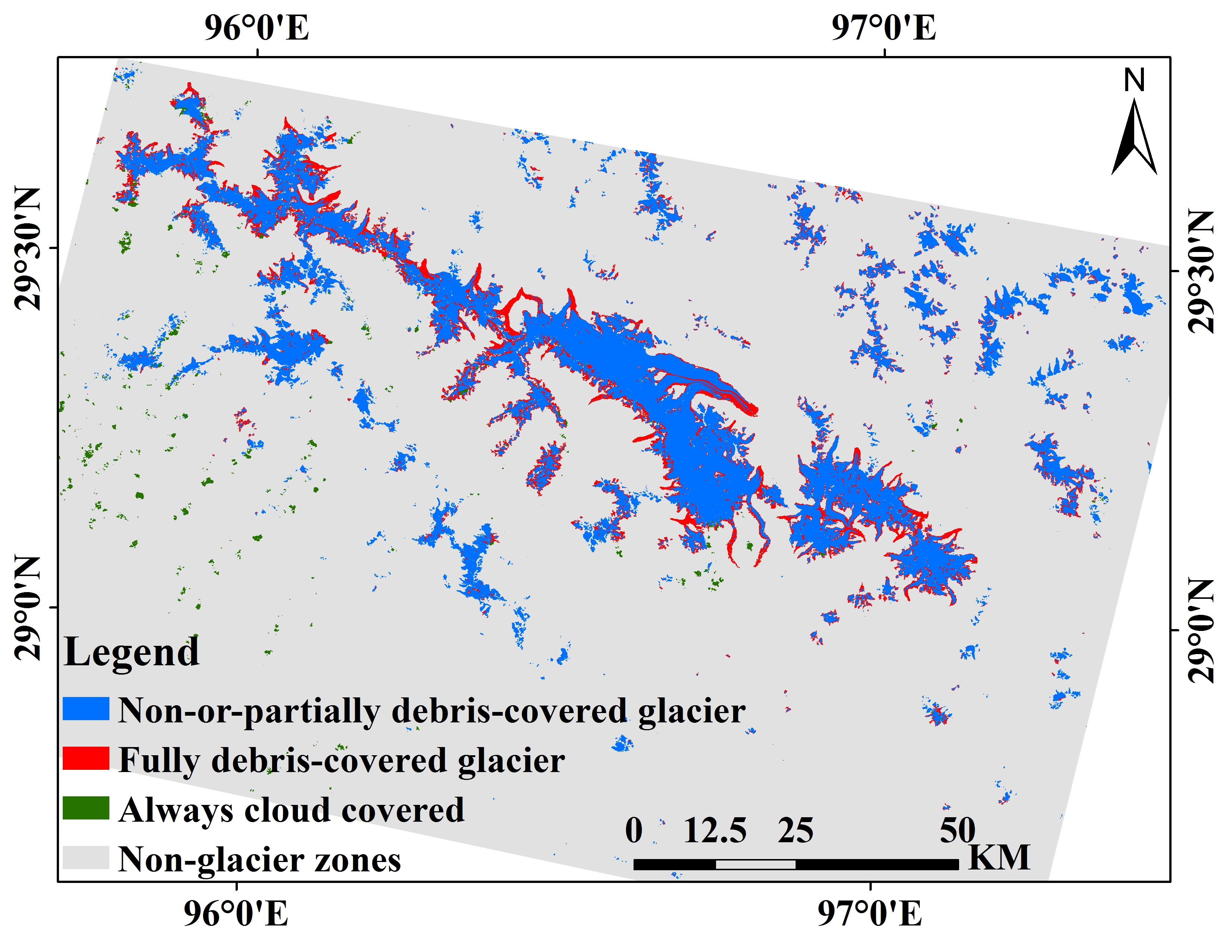
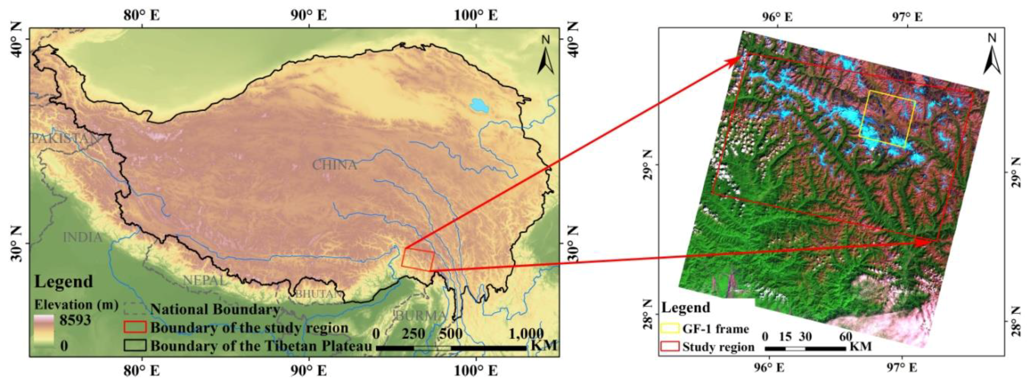
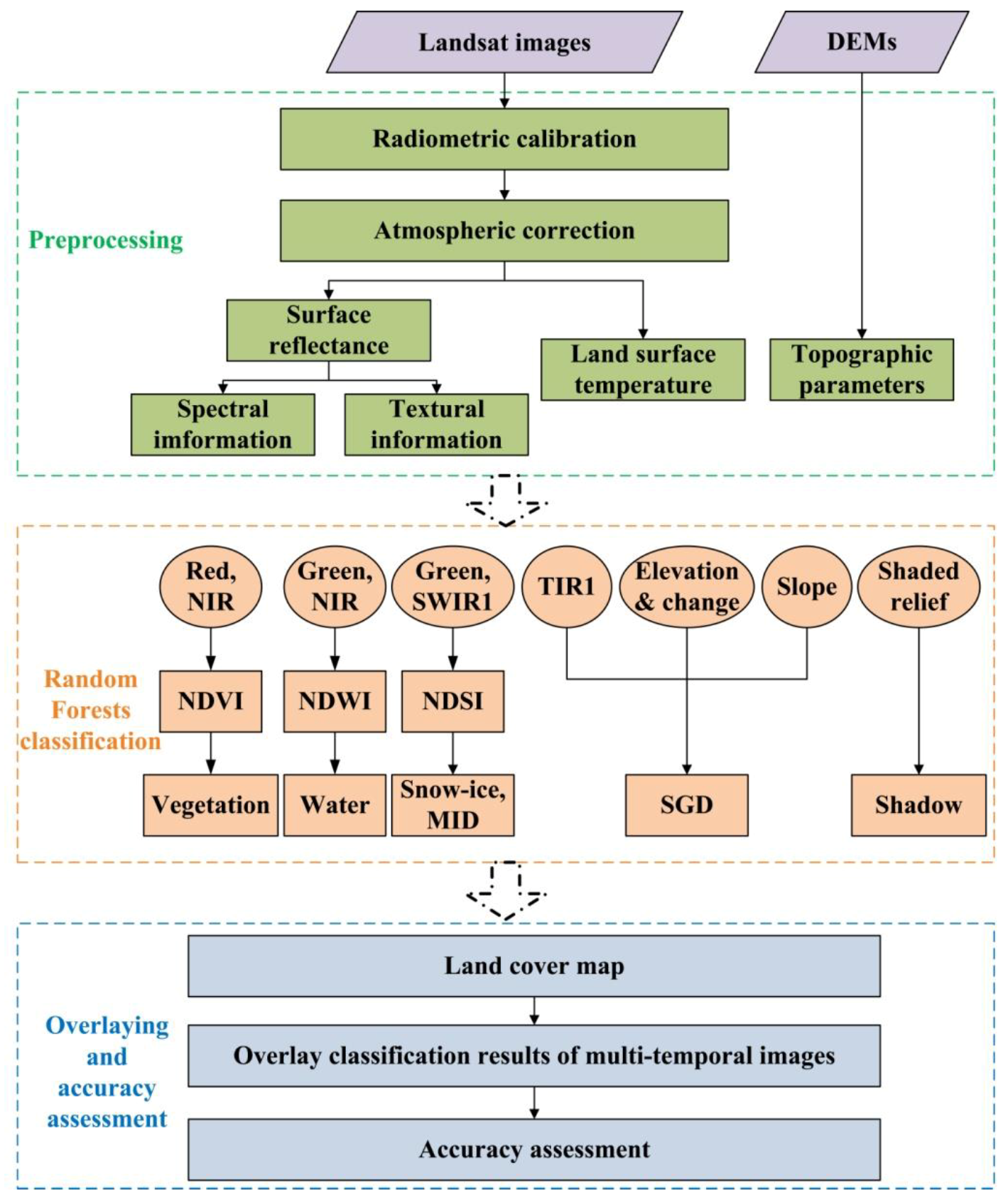
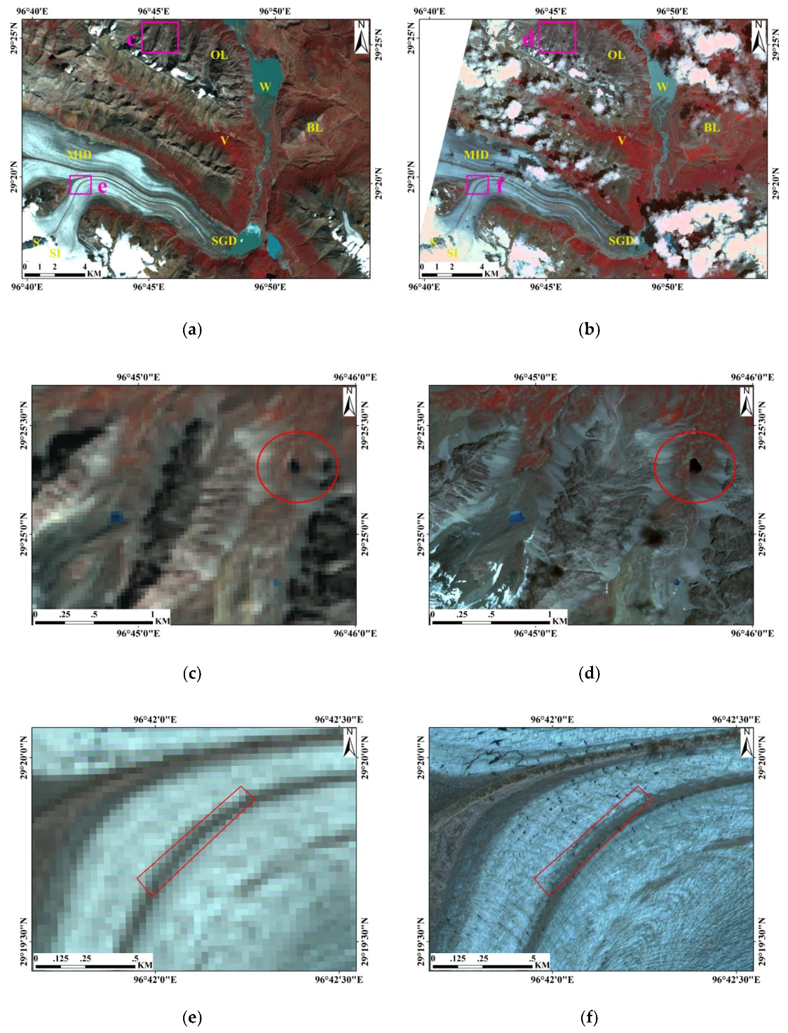
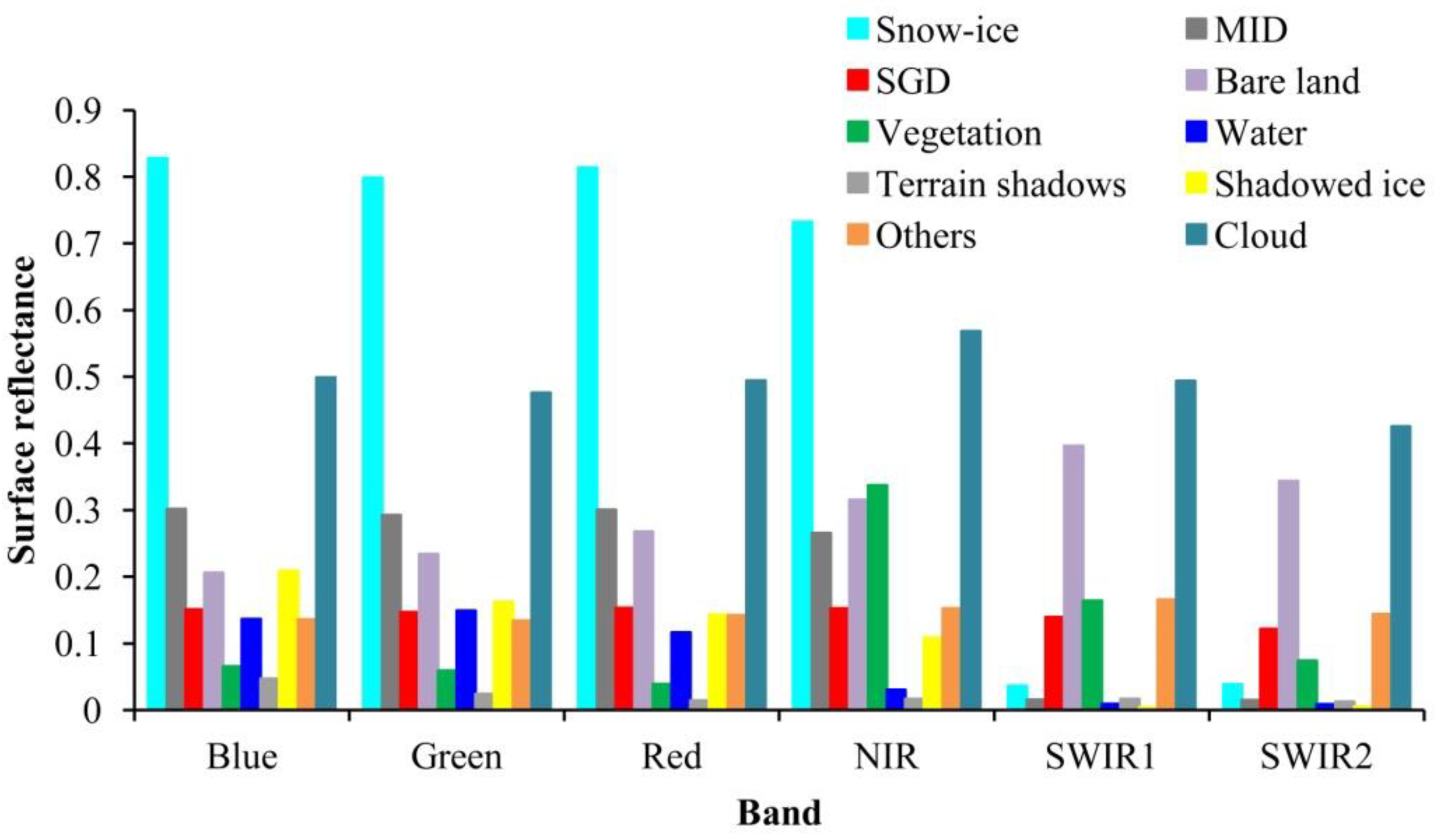
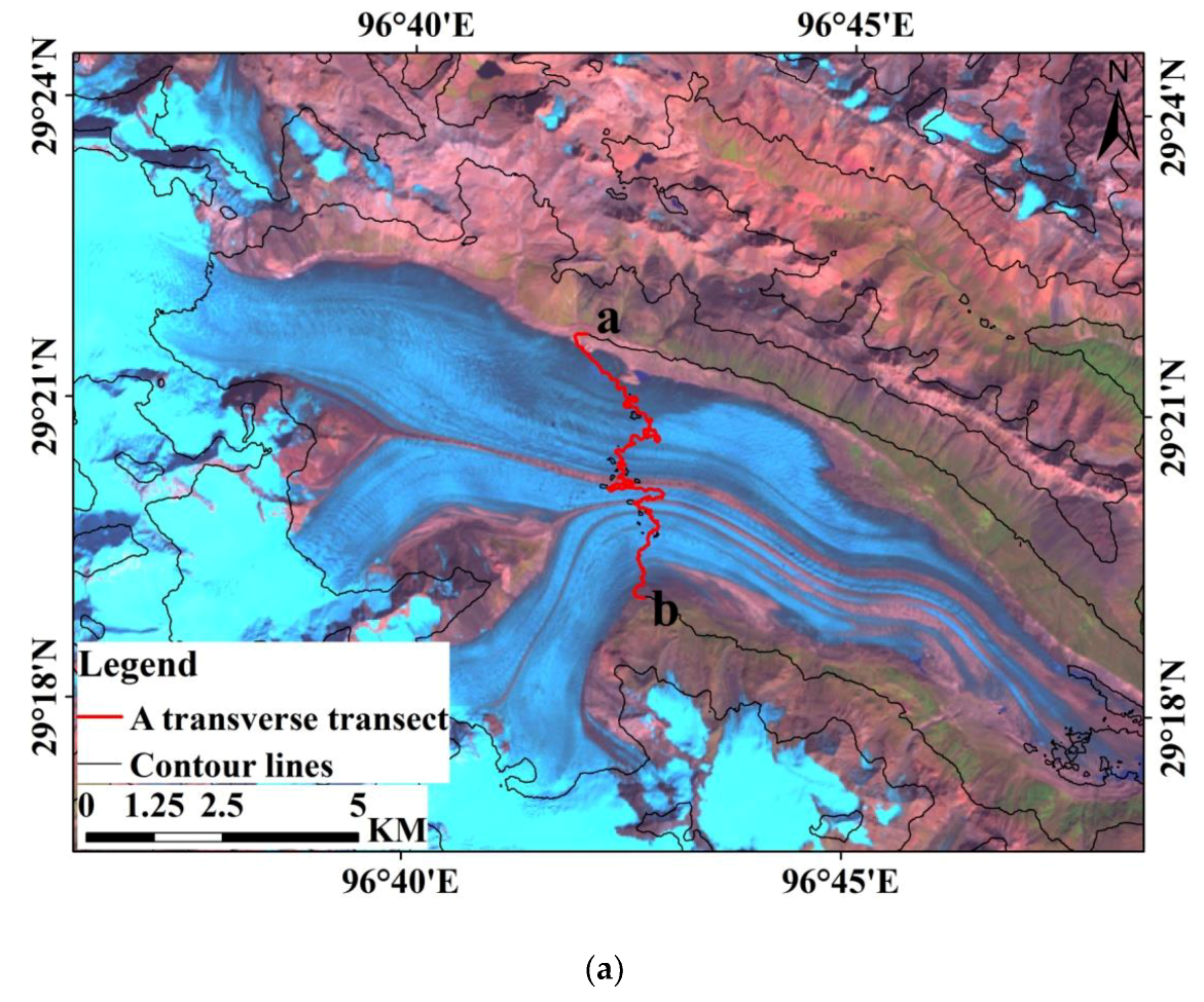
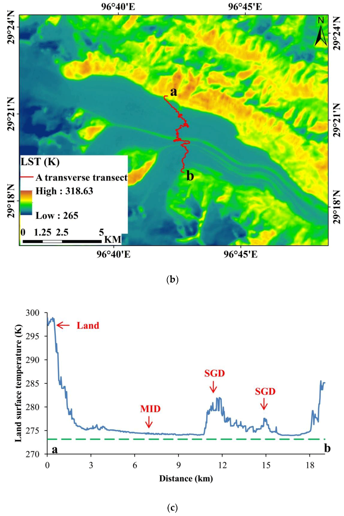
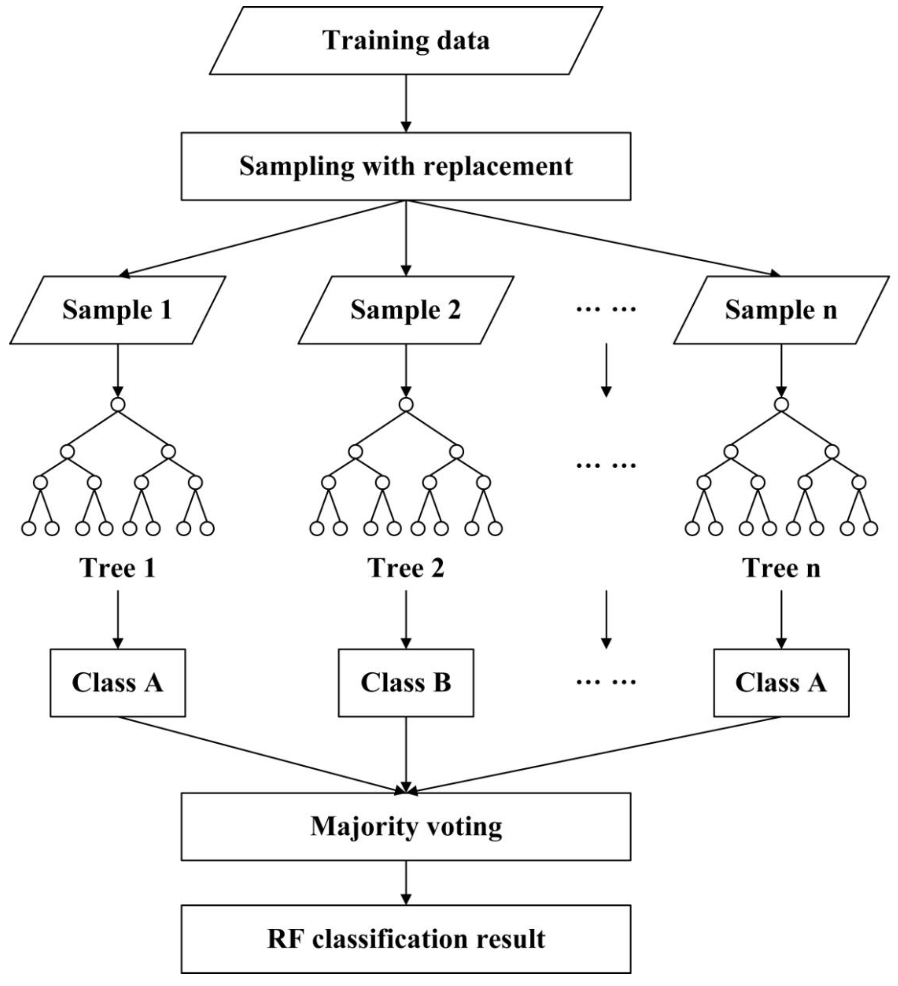
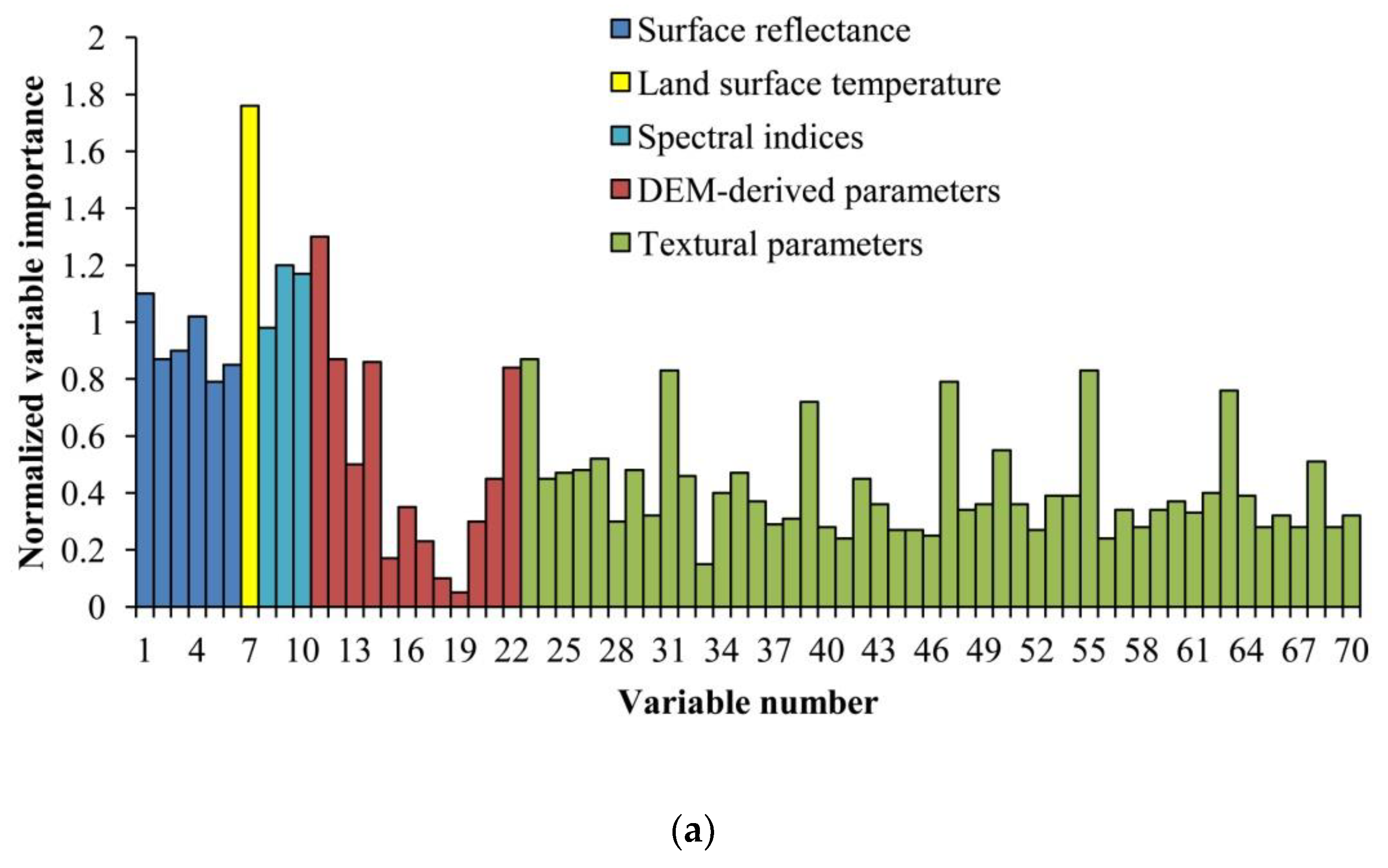
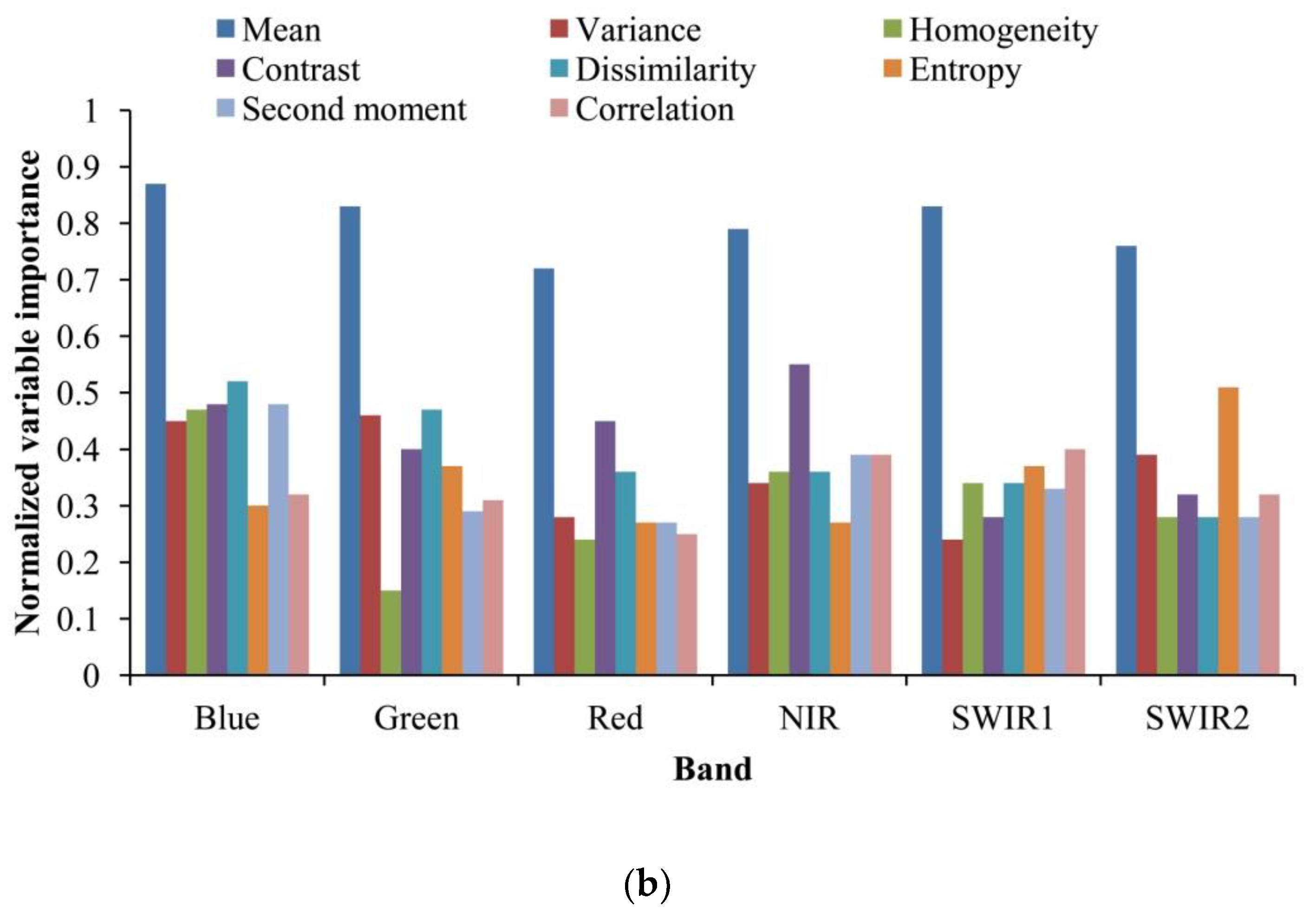
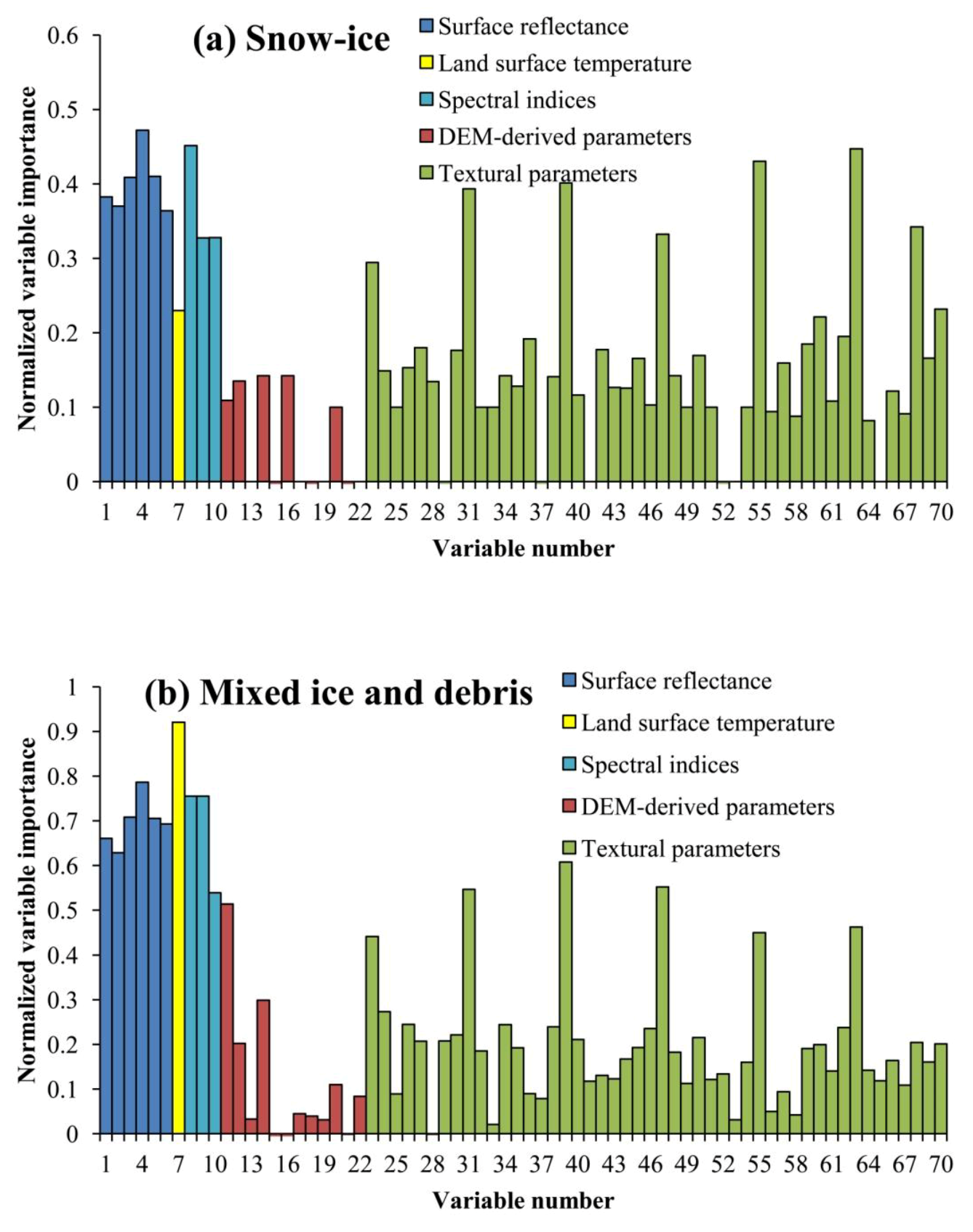
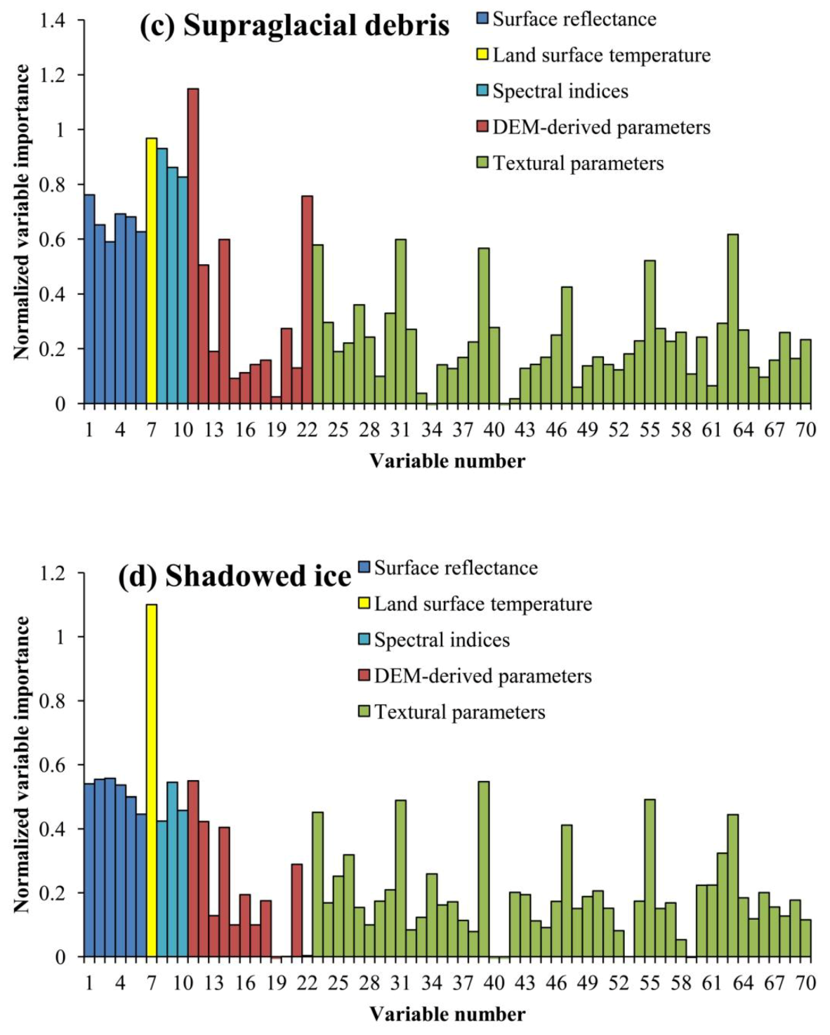
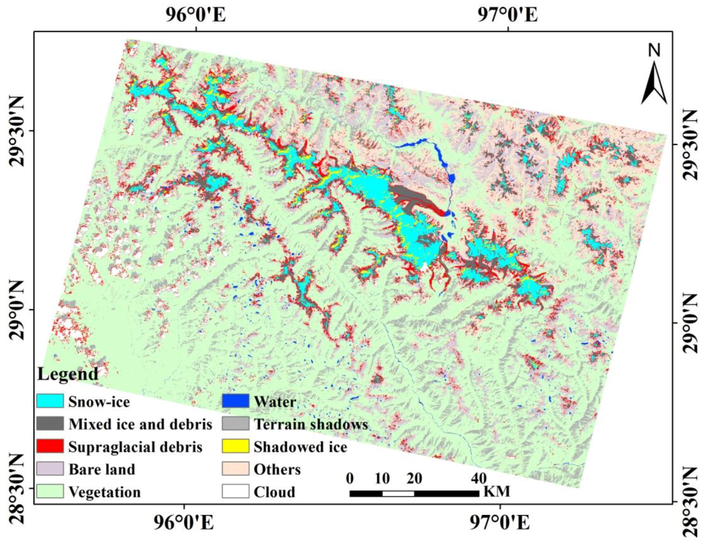
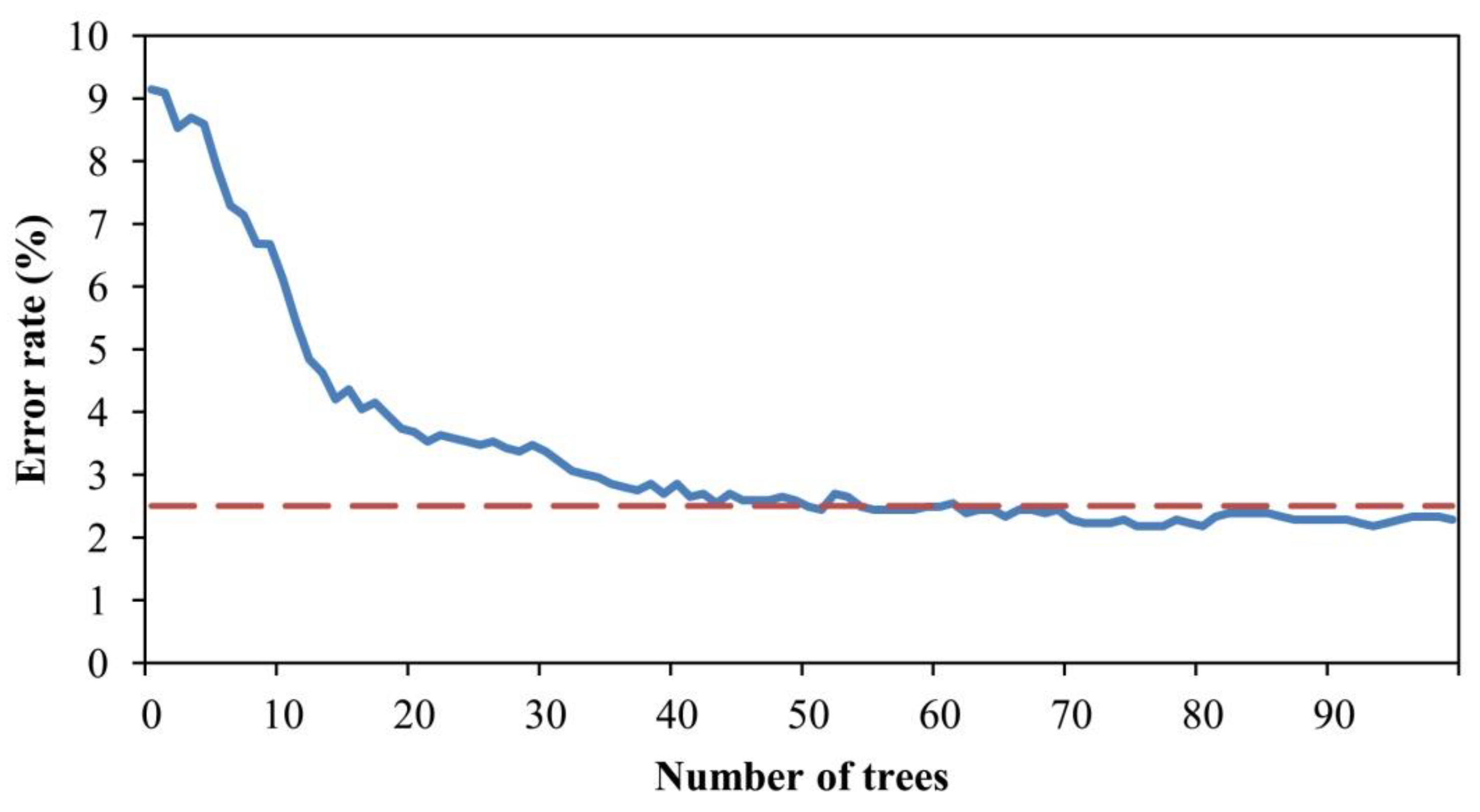
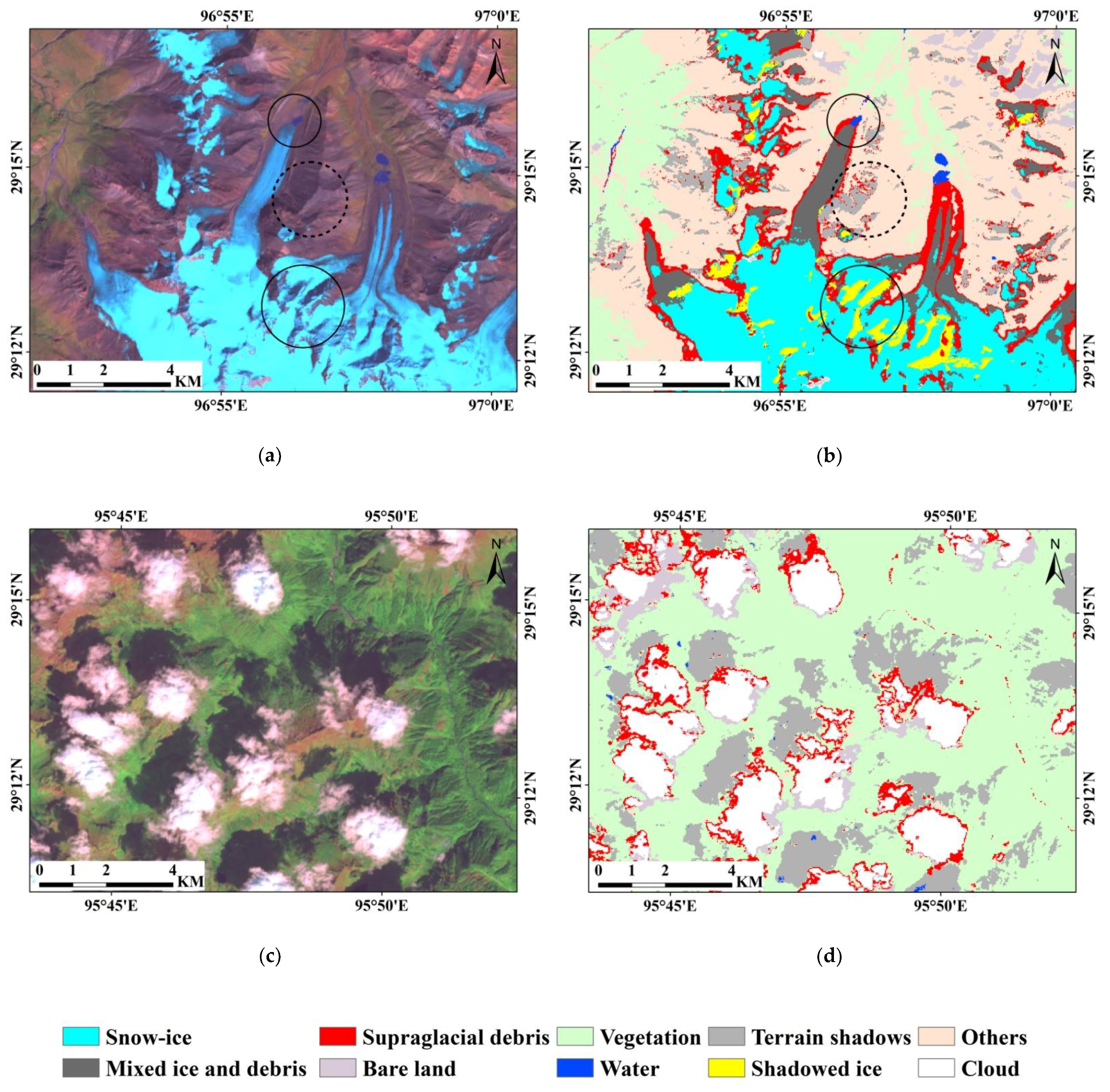
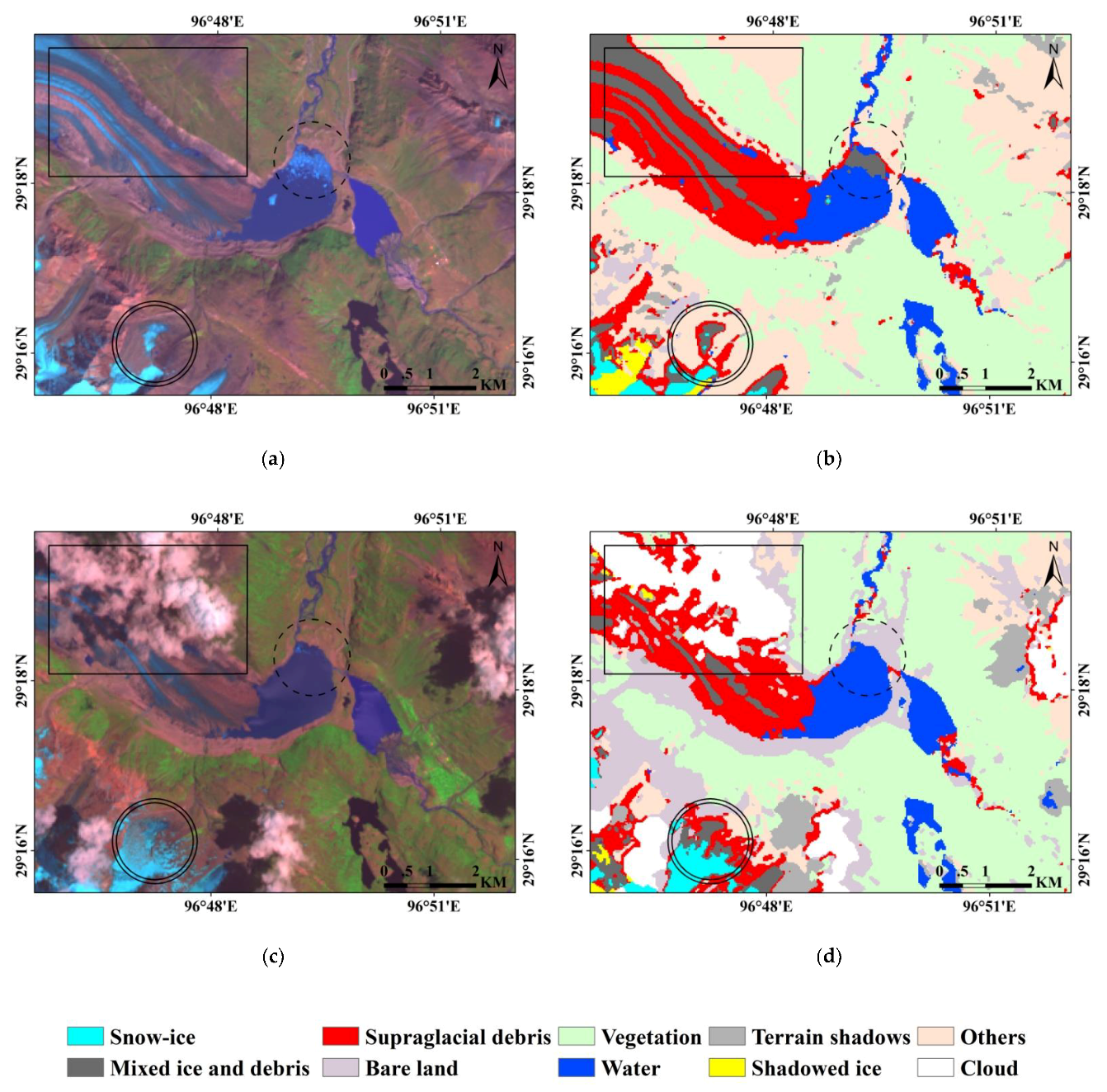
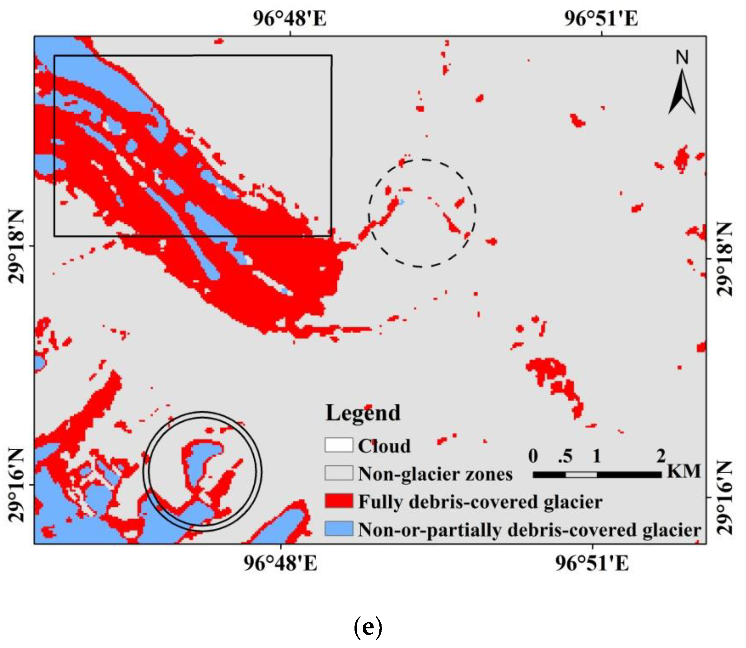
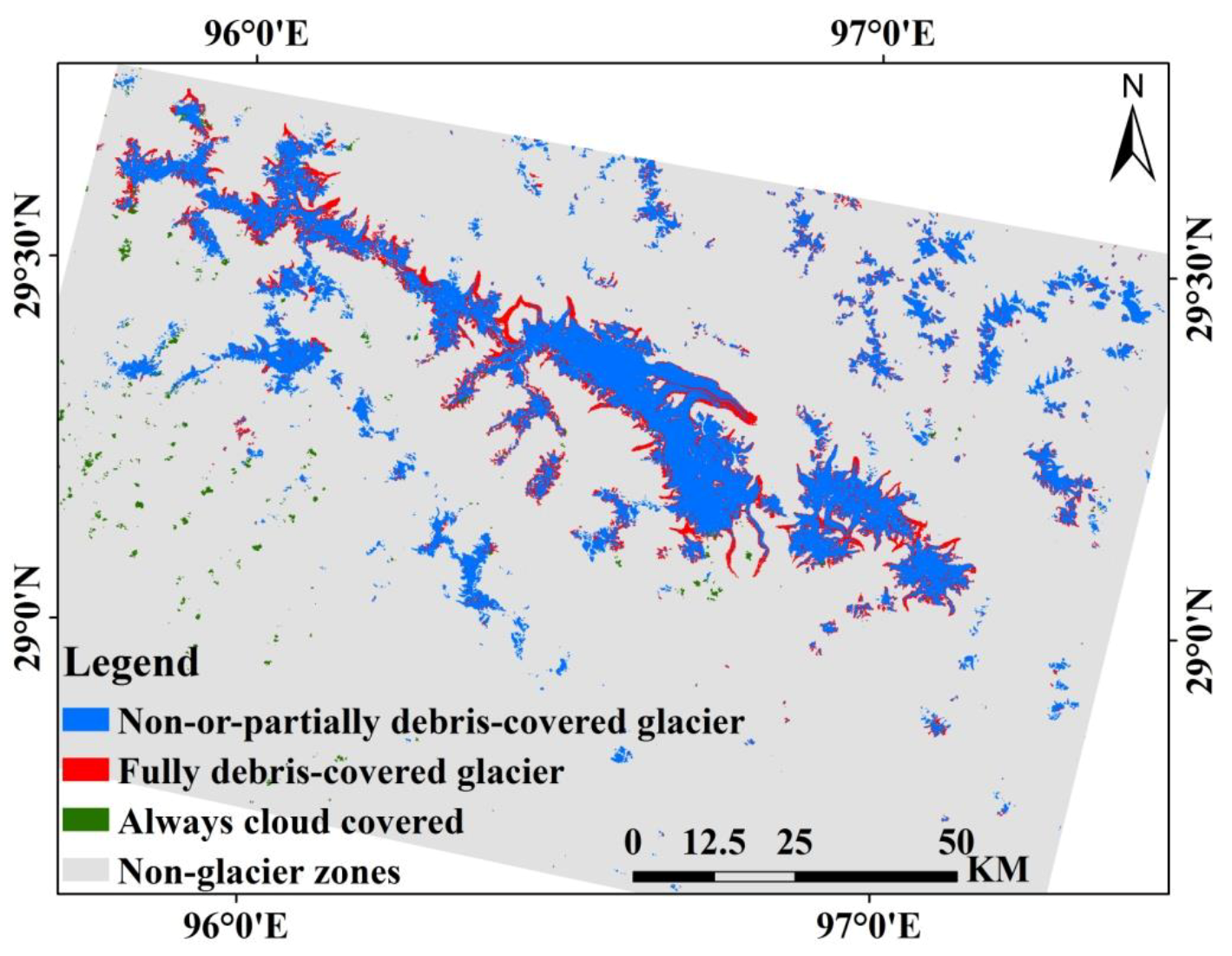
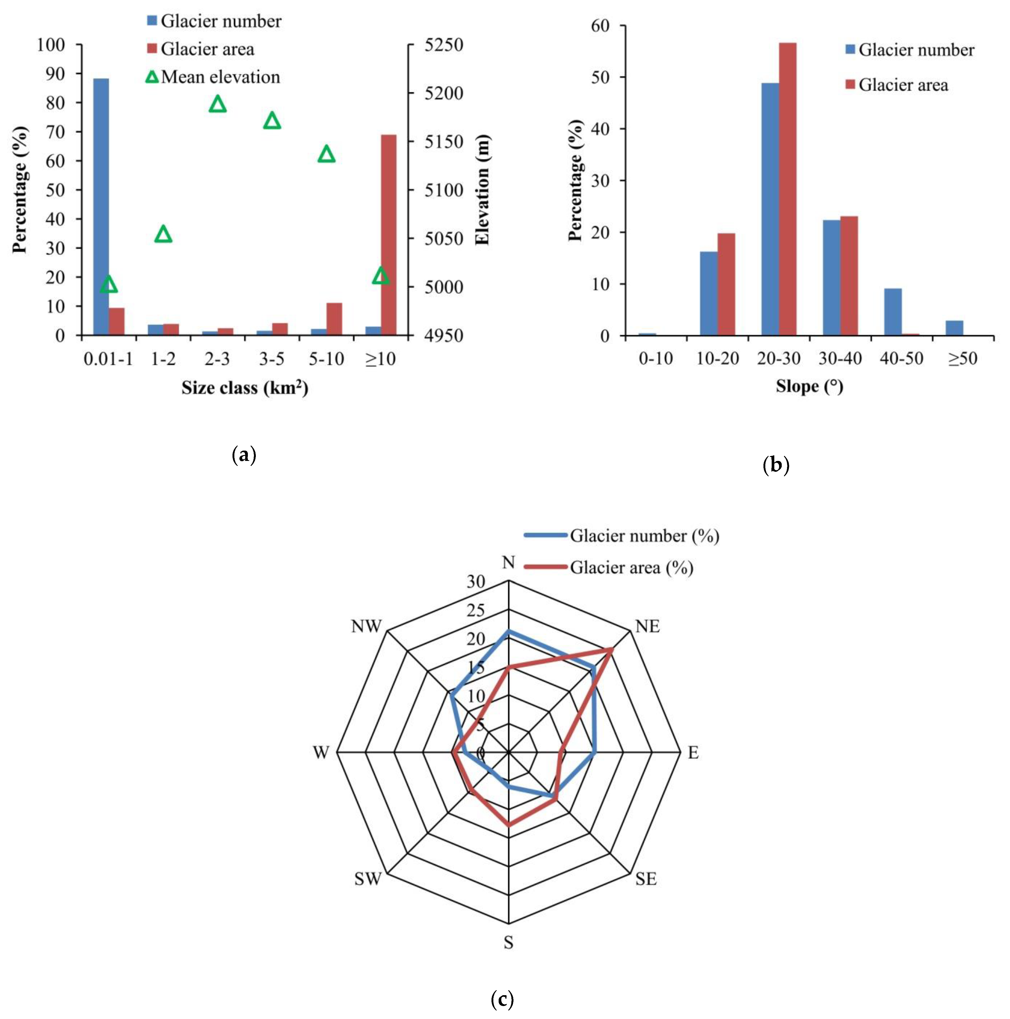
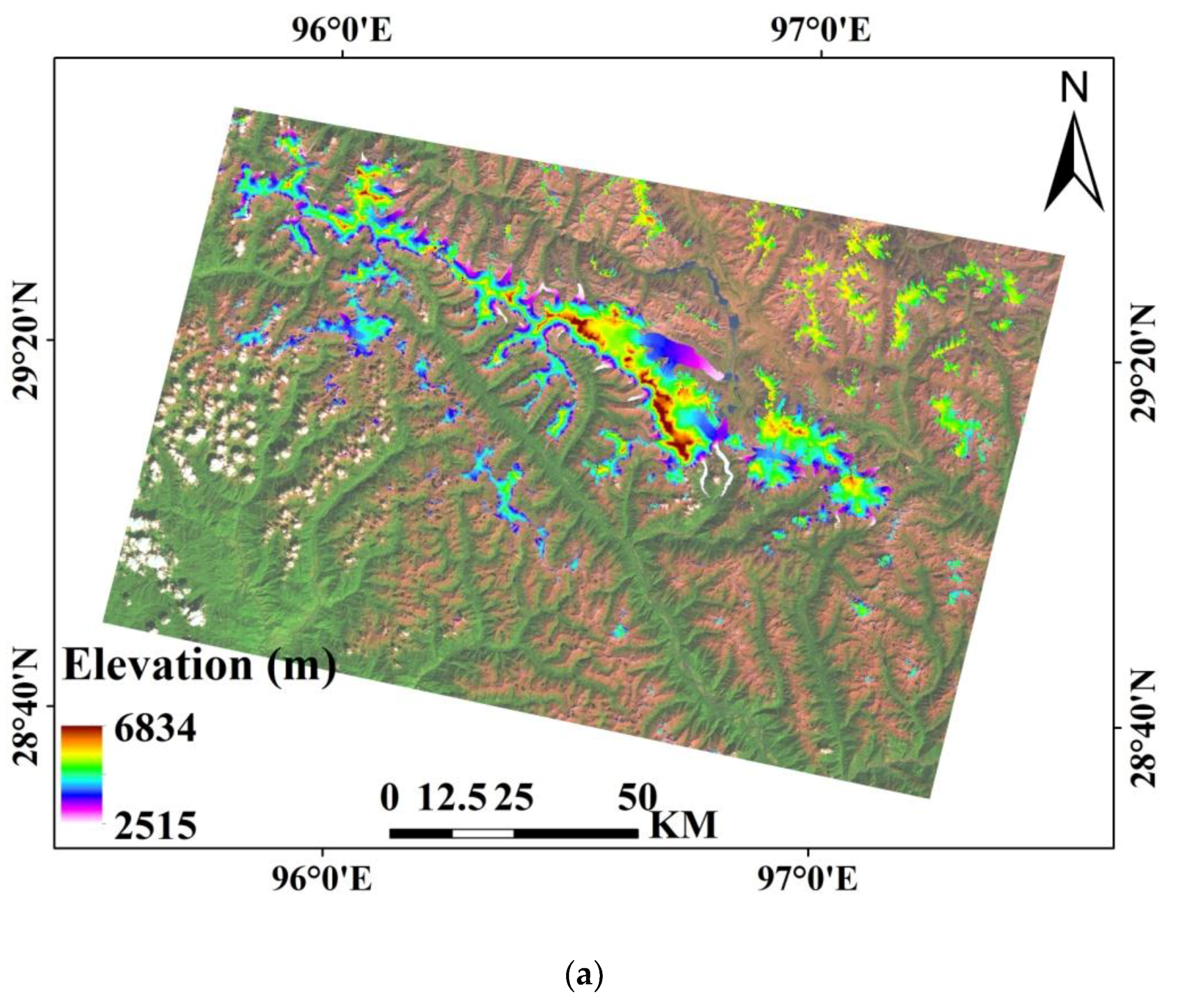
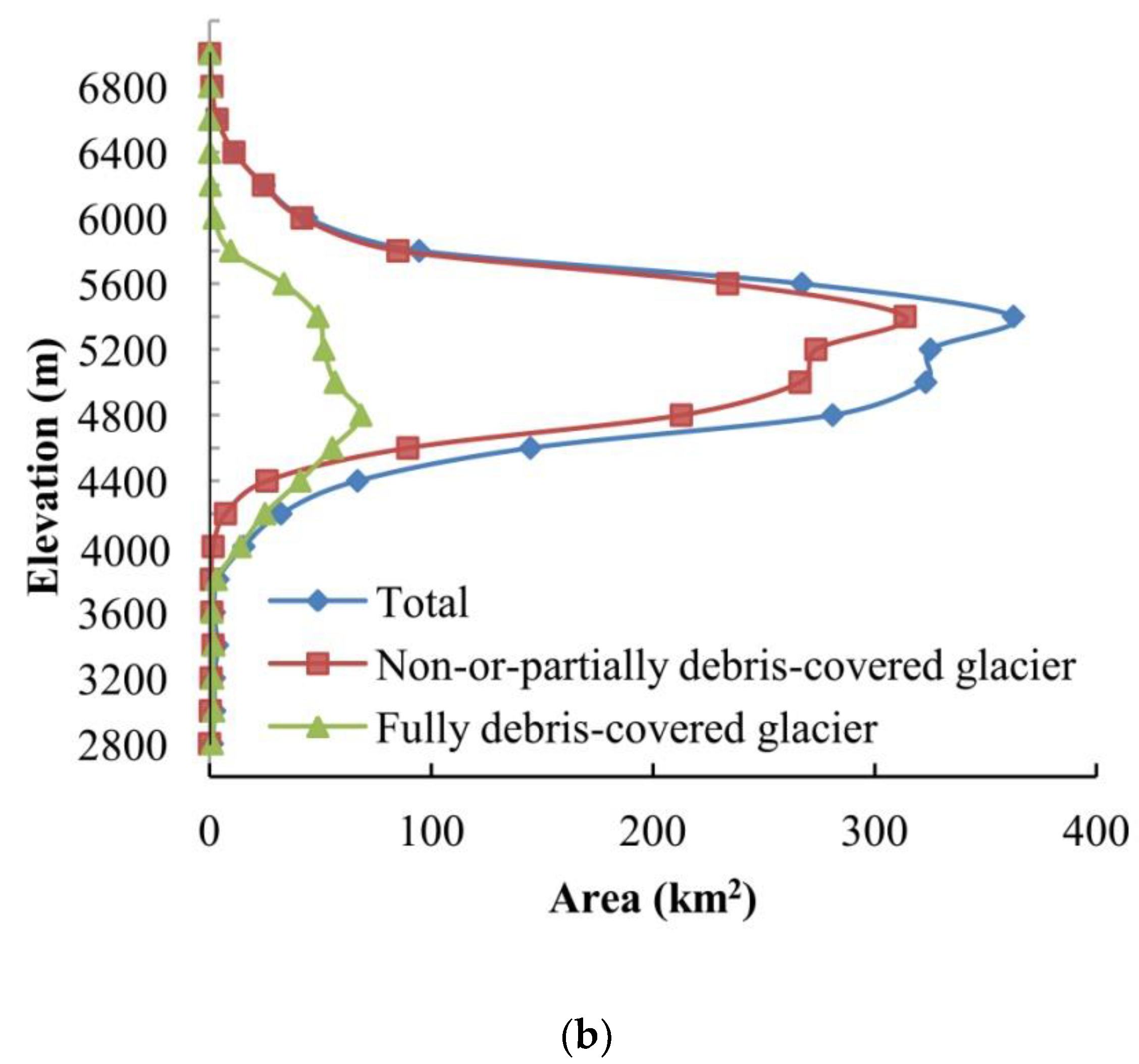
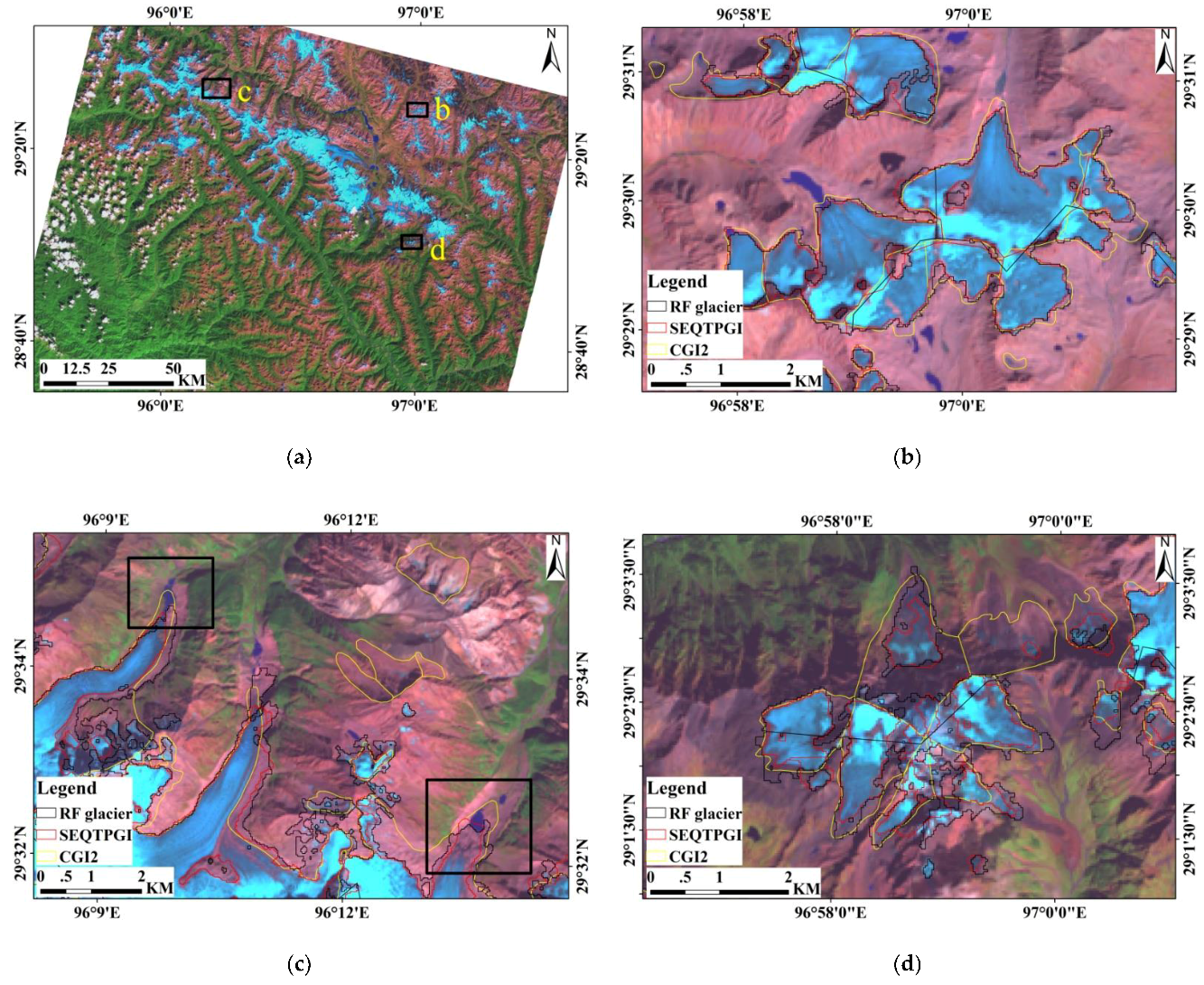
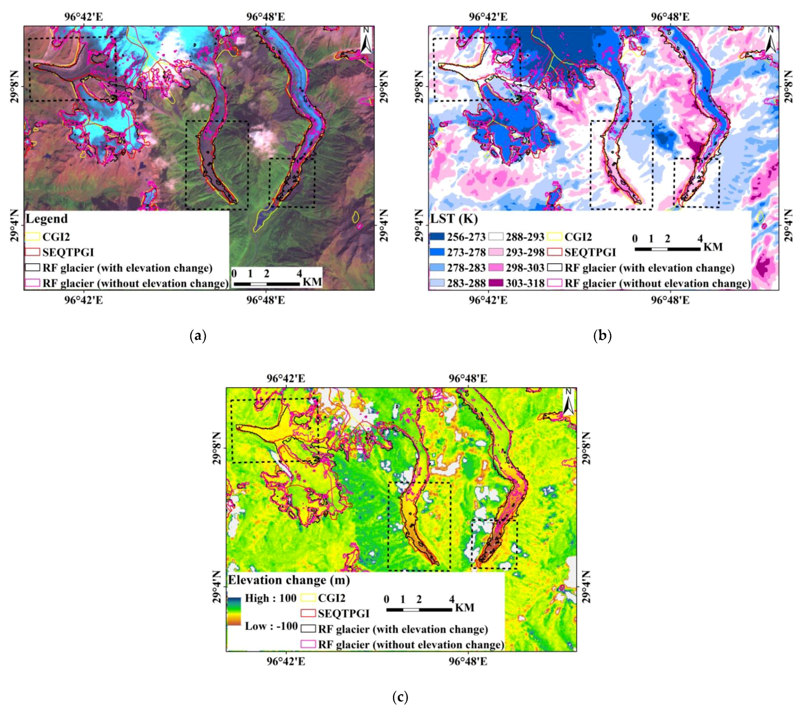
Table 1.
A list of OLI and Thermal Infrared Sensor (TIRS) spectral bands of Landsat-8.
| Band Number | Band Number | Bandpass (μm) | Spatial Resolution (m) |
|---|---|---|---|
| 1 | Coastal/Aerosol | 0.435–0.451 | 30 |
| 2 | Blue | 0.452–0.512 | 30 |
| 3 | Green | 0.533–0.590 | 30 |
| 4 | Red | 0.636–0.673 | 30 |
| 5 | NIR | 0.851–0.879 | 30 |
| 6 | SWIR 1 | 1.566–1.651 | 30 |
| 7 | SWIR 2 | 2.107–2.294 | 30 |
| 8 | PAN | 0.503–0.676 | 15 |
| 9 | Cirrus | 1.363–1.384 | 30 |
| 10 | TIR 1 | 10.60–11.19 | 100 |
| 11 | TIR 2 | 11.50–12.51 | 100 |
NIR, near-infrared; SWIR, shortwave infrared; PAN, panchromatic; TIR, thermal infrared.
Table 2.
A list of the Landsat-8 images used in this study.
| Image Number | Date of Acquisition | Cloud Coverage (%) |
|---|---|---|
| 1 | 18 July 2015 | 46 |
| 2 | 6 October 2015 | 6 |
| 3 | 22 October 2015 | 26 |
Table 3.
The land surface emissivity estimation algorithm based on the Normalized Difference Snow Index (NDSI) and Normalized Difference Vegetation Index (NDVI) image.
Table 3.
The land surface emissivity estimation algorithm based on the Normalized Difference Snow Index (NDSI) and Normalized Difference Vegetation Index (NDVI) image.
| Threshold | Land Cover | LSE |
|---|---|---|
| NDSI > 0.4 | Ice | A constant value of ice emissivity |
| (NDSI ≤ 0.4) and (NDVI < NDVIs) | Bare soil | An empirical relationship with the red band reflectance [47,53] |
| (NDSI ≤ 0.4) and (NDVI > NDVIv) | Fully vegetated | A constant value of vegetation emissivity |
| (NDSI ≤ 0.4) and (NDVIs ≤ NDVI ≤ NDVIv 1) | A mixture of bare soil and vegetation | 2 |
1 NDVIs and NDVIv are the threshold values distinguishing soil and vegetation cover, respectively, which can be extracted from the NDVI histogram. 2 where is the vegetation emissivity, is the soil emissivity, Pv is the vegetation fraction derived from the NDVI, and dε reveals the influence of the geometrical distribution of the natural surfaces [47]. LSE, land surface emissivity.
Table 4.
The topographic features extracted from multiple DEM data.
| Topographic Feature | Description |
|---|---|
| Elevation | The height above a given level, especially sea level. |
| Slope | Calculated with the convention of 0 degrees for a horizontal plane. |
| Aspect | Aspect angle is the convention of 0 degrees to the north (up) and angles increasing clockwise. |
| Shaded relief | Shaded relief shows an apparent three-dimensional configuration of the shape of terrain. |
| Profile convexity | The change rate of the slope along the profile. |
| Plane convexity | The change rate of the aspect along the plane. |
| Longitudinal convexity | The surface curvature orthogonally in the down slope direction. |
| Cross-sectional convexity | The surface curvature orthogonally in the across slope direction. |
| Minimum curvature | The minimum surface curvatures. |
| Maximum curvature | The maximum surface curvatures. |
| Root-mean-square error | Generated to indicate how well the quadratic surface fits the actual DEM data and calculated in a neighborhood (3 × 3 pixels) around each pixel [70]. |
| Absolute elevation change | The magnitude of the absolute change of surface elevation |
Table 5.
Textural features extracted from the Grey Level Co-occurrence Matrix (GLCM).
| Textural Feature | Description | Formula 1 |
|---|---|---|
| Mean | Gray level average in the GLCM, not the mean of the original pixel values (band reflectance) within the given window size (3 × 3 grid cell). | |
| Variance | Gray level variance in the GLCM. | |
| Homogeneity | Homogeneity is a measure of the homogenous gray level across an image. It is high when local pixel values are uniform. | |
| Contrast | Contrast measures the amount of local variation in pixel values among neighboring pixels. Contrast is zero when the neighboring pixels have constant values [72]. | |
| Dissimilarity | Similar to contrast and inversely related to homogeneity [73]. | |
| Entropy | Entropy measures the disorder or complexity of an image. It is high when the pixel values of the GLCM are varying and it is the opposite of the angular second moment. | |
| Angular second moment | Angular second moment measures the image uniformity. It is high when the pixel values of the GLCM are very similar. | |
| Correlation | Correlation is the gray-scale measure of the linear relationship, and it measures the linear dependency of pixel values on those of neighboring pixels in the GLCM [74]. |
1 where i and j are coordinates of the GLCM, p(i,j) refers to the value at the (i,j)th position in the GLCM, and μ and σ represent the means and standard deviations of px and py [71].
Table 6.
The area for each land cover class obtained by the RF classifier.
| Land Cover Class | Area (km2) | Percent (%) |
|---|---|---|
| Snow-ice | 821.49 | 4.4 |
| Mixed ice and debris | 677.12 | 3.6 |
| Supraglacial debris | 959.84 | 5.1 |
| Bare land | 1608.53 | 8.6 |
| Vegetation | 9915.22 | 52.8 |
| Water | 134.39 | 0.7 |
| Terrain shadows | 2025.88 | 10.8 |
| Shadowed ice | 161.75 | 0.9 |
| Others | 2116.68 | 11.3 |
| Cloud | 358.02 | 1.9 |
| Total | 18,778.92 | 100 |
Table 7.
The confusion matrix and accuracy assessment of the land cover classification results.
| Confusion Matrix | Reference | |||||||||||
|---|---|---|---|---|---|---|---|---|---|---|---|---|
| Snow-Ice | Mixed Ice and Debris | Supraglacial Debris | Bare Land | Vegetation | Water | Terrain Shadows | Shadowed Ice | Others | Cloud | User’s Accuracy (%) | ||
| Classified | Snow-ice | 99.2 | 0 | 0 | 0 | 0 | 0 | 0 | 0 | 0 | 0 | 100 |
| Mixed ice and debris | 0.8 | 100 | 0 | 0 | 0 | 0 | 0 | 0 | 0 | 0 | 98.8 | |
| Supraglacial debris | 0 | 0 | 98.7 | 0 | 0 | 0 | 0 | 0 | 10.9 | 0 | 93.9 | |
| Bare land | 0 | 0 | 0 | 100 | 0 | 0 | 0 | 0 | 0 | 2.6 | 97.6 | |
| Vegetation | 0 | 0 | 0 | 0 | 96.5 | 0 | 0 | 0 | 0 | 0 | 100 | |
| Water | 0 | 0 | 0 | 0 | 0 | 100 | 1 | 0 | 0 | 0 | 98.8 | |
| Terrain shadows | 0 | 0 | 0 | 0 | 3.5 | 0 | 99 | 0 | 0 | 0 | 98.1 | |
| Shadowed ice | 0 | 0 | 0 | 0 | 0 | 0 | 0 | 100 | 0 | 0 | 100 | |
| Others | 0 | 0 | 1.3 | 0 | 0 | 0 | 0 | 0 | 89.1 | 0 | 97.6 | |
| Cloud | 0 | 0 | 0 | 0 | 0 | 0 | 0 | 0 | 0 | 97.4 | 100 | |
| Total | 100 | 100 | 100 | 100 | 100 | 100 | 100 | 100 | 100 | 100 | Total (%): 98.6 | |
| Producer’s Accuracy (%) | 99.3 | 100 | 98.7 | 100 | 96.5 | 100 | 99 | 100 | 89.1 | 97.4 | ||
© 2019 by the authors. Licensee MDPI, Basel, Switzerland. This article is an open access article distributed under the terms and conditions of the Creative Commons Attribution (CC BY) license (http://creativecommons.org/licenses/by/4.0/).
Share and Cite
MDPI and ACS Style
Zhang, J.; Jia, L.; Menenti, M.; Hu, G. Glacier Facies Mapping Using a Machine-Learning Algorithm: The Parlung Zangbo Basin Case Study. Remote Sens. 2019, 11, 452. https://0-doi-org.brum.beds.ac.uk/10.3390/rs11040452
AMA Style
Zhang J, Jia L, Menenti M, Hu G. Glacier Facies Mapping Using a Machine-Learning Algorithm: The Parlung Zangbo Basin Case Study. Remote Sensing. 2019; 11(4):452. https://0-doi-org.brum.beds.ac.uk/10.3390/rs11040452
Chicago/Turabian StyleZhang, Jingxiao, Li Jia, Massimo Menenti, and Guangcheng Hu. 2019. "Glacier Facies Mapping Using a Machine-Learning Algorithm: The Parlung Zangbo Basin Case Study" Remote Sensing 11, no. 4: 452. https://0-doi-org.brum.beds.ac.uk/10.3390/rs11040452
Note that from the first issue of 2016, this journal uses article numbers instead of page numbers. See further details here.