Crop Classification Based on a Novel Feature Filtering and Enhancement Method


1
Institute of Agricultural Resources and Regional Planning, Chinese Academy of Agricultural Sciences, Beijing 100081, China
2
Key Laboratory of Agri-informatics, Ministry of Agriculture, Beijing 100081, China
3
Department of Remote Sensing, Flemish Institute of Technological Research, 2400 Mol, Belgium
4
Institute of Applied Remote Sensing and Information Technology, Zhejiang University, Hangzhou 310058, China
5
Key Laboratory of Agricultural Remote Sensing and Information Systems, Zhejiang University, Hangzhou 310058, China
*
Author to whom correspondence should be addressed.
Remote Sens. 2019, 11(4), 455; https://0-doi-org.brum.beds.ac.uk/10.3390/rs11040455
Submission received: 6 January 2019
/
Revised: 19 February 2019
/
Accepted: 19 February 2019
/
Published: 22 February 2019
(This article belongs to the Special Issue Remote Sensing in Support of Transforming Smallholder Agriculture)
Abstract
:Vegetation indices, such as the normalized difference vegetation index (NDVI) or enhanced vegetation index (EVI) derived from remote sensing images, are widely used for crop classification. However, vegetation index profiles for different crops with a similar phenology lead to difficulties in discerning these crops both spectrally and temporally. This paper proposes a feature filtering and enhancement (FFE) method to map soybean and maize, two major crops widely cultivated during the summer season in Northeastern China. Different vegetation indices are first calculated and the probability density functions (PDFs) of these indices for the target classes are established based on the hypothesis of normal distribution; the vegetation index images are then filtered using the PDFs to obtain enhanced index images where the pixel values of the target classes are ”enhanced”. Subsequently, the minimum Gini index of each enhanced index image is computed, generating at the same time the weight for every index. A composite enhanced feature image is produced by summing all indices with their weights. Finally, a classification is made from the composite enhanced feature image by thresholding, which is derived automatically based on the samples. The efficiency of the proposed FFE method is compared with the maximum likelihood classification (MLC), support vector machine (SVM), and random forest (RF) in a mapping operation to determine the soybean and maize distribution in a county in Northeastern China. The classification accuracies resulting from this comparison show that the FFE method outperforms MLC, and its accuracies are similar to those of SVM and RF, with an overall accuracy of 0.902 and a kappa coefficient of 0.846. This indicates that the FFE method is an appropriate method for crop classification to distinguish crops with a similar phenology. Our research also shows that when the sample size reaches a certain level (e.g., 2000), the mean and standard deviation of the sample are very close to the actual values, which leads to high classification accuracy. In a case where the condition of normal distribution is not fulfilled, the PDF of the vegetation index can be created by a lookup table. Furthermore, as the method is rather simple and explicit, and convenient in terms of computing, it can be used as the backbone for automatic crop mapping operations.
1. Introduction
The conventional means of acquiring information about crop planting areas include field survey and statistics sampling as well as remote sensing image analysis. For example, using remote sensing data, the US National Agricultural Statistics Service (NASS) established a sampling frame for agricultural statistics, estimated crop planting areas and offered crop-oriented land cover data for an analytic system [1,2]. In the LUCAS (land use/cover area—frame survey) project in the European Union, the crop planting area and yield were estimated by means of area frame sampling [3]. These methods are considered accurate and objective, with disadvantages in terms of resource requirements [4]. In addition to this, they cannot provide precise spatial distribution information for crop areas.
Remote sensing mapping has the advantages of larger area coverage and low cost and, therefore, a relatively high efficiency [5,6]. In recent years, high-resolution imagery (Landsat-8, Sentinel-2, Gaofeng-1, etc.) has become the main data source to derive crop area information [7,8,9,10,11,12]. Different classification methods or their improvements have been routinely applied including maximum likelihood classification (MLC), support vector machine (SVM), random forest (RF), neural networks (NNs), and so on [12,13,14,15,16]. For example, the SVM method is considered to be suitable for dealing with small data samples and has been widely used in remote sensing-based crop classification [17,18,19]; RF is another state-of-the-art machine learning method and is considered to be effective in avoiding over-fitting, and has the advantages of being accurate and efficient [20,21,22]. A review of machine learning classification methods was proposed by Holloway and Mengersen [23]. One of their conclusions is that there is usually no one true or correct approach, but it is of interest to consider approaches for selecting an appropriate method for a given problem. However, most of these machine learning methods are considered as ‘black boxes’, in which the specific crop classification processes are fuzzy, which requires a great deal of experience to optimize the classification model parameters and to improve the classification accuracy. Another classification method is to construct decision trees based on expert knowledge and classify crops by setting some decision rules artificially based on the features of ground objects [24]. The classification mechanism of this method is clear and easy to understand, and has been widely used in crop classification. Nevertheless, the construction of classification rules may be difficult for classes with similar phenology. Therefore, a series of indices are proposed to enhance the difference between different classes. For example, the normalized differential vegetation index (NDVI) could improve the difference between vegetation and non-vegetation, and the normalized difference water index (NDWI) could improve the difference between water and other objects [25,26,27]. Wardlow and Egbert [28] completed the mapping of crops in Southeast Kansas by using the NDVI and EVI time series data of Moderate-resolution Imaging Spectroradiometer (MODIS) and obtained a high accuracy of 85% to 90%; Mansaray et al. [29] computed the NDVI and MNDWI (modified normalized difference water index) from Landsat-8 and Sentinel-1A imagery and produced a high-accurate paddy rice distribution map based on the decision tree approach.
Moreover, to efficiently resolve the problem of misclassification due to similar crop phenology, different approaches to enhance the features (or variable) of target classes and improve the classification accuracy have been proposed. Li et al. [30] reported a texture feature enhancement (TFE) method to improve the texture features of hyperspectral data, and then deep belief networks (DBNs) were employed on hyperspectral reconstructed data for classification. They found that, after using the TFE method, the texture features of the hyperspectral image became more obvious and clear, and the classification accuracies were increased. Zhang et al. [31] published a block-based synthetic variable ratio (block-SVR) method aimed at a pixel-level fusion for optical and synthetic aperture radar (SAR) images to combine these two types of remotely-sensed imagery for feature enhancement. The study indicated that the larger the regression block, the more the spatial and textural features were enhanced. Nevertheless, all these approaches focused on specific types of image data, such as hyperspectral or SAR images, and none of them was aimed at enhancing the spectral or index features of multi-spectral remote sensing data.
Due to the similar spectral profiles of crops, it is always interesting to enhance the spectral difference between different crop classes in remote sensing images. This paper proposes a novel feature filtering and enhancement (FFE) method based on probability density functions (PDFs). Different indices are computed from raw images, and the PDFs are then calculated and used to filter the image and enhance the difference between the target class and background. In this way, the index value of the target class is maximized. Four index features—normalized difference vegetation index (NDVI), modified normalized difference water index (MNDWI), the mean of Shortwave Infrared (SWIR) bands (SWIRmean) and visible light index (VLI)—are included in this investigation. A weighted addition method based on the Gini index is used to combine all the enhanced images together and generate a single image (called the composite enhanced feature image, or CEF image) in which the pixels of the target class have much higher values than those of other classes. Thus, a single threshold could be used to distinguish the target class and background classes. In this case, classes of maize and soybean are identified based on the CEF images. Finally, the performance of the FFE method is compared with the MLC, SVM and RF methods. In order to evaluate the relationship between sample size and PDF approximation, a series of sample sets with different sample size are used to generate the PDFs of soybean, and then compare these with the actual PDFs which are calculated from all soybean pixels. Moreover, a look-up-table (LUT) method is used to generate PDFs in cases when the features are not normally distributed, and the accuracy of LUT-based FFE classification is also discussed.
2. Study Site and Data
2.1. Study Site
To test the FFE method, a study area located within Bei’an county in Heilongjiang, a northeastern province of China, was selected, see Figure 1. The area situated between the Songnen Plain and Greater Khingan Range is characterized by the presence of black soil, which is particularly suitable for grain cultivation, as well, of course, as weather conditions which are very favorable for agriculture. Soybean and maize, respectively, take up approximately 29% and 59% of the total sowing area of grains in the area [32].
2.2. Phenology of Maize and Soybean
The phenology of maize and soybean in the study site is related to the sowing date, sunlight duration, accumulated temperature, and rainfall. The period may vary slightly from one year to another including sowing, emerging, three-leaf, seven-leaf, jointing, tasseling, milk ripening, and ripening. Maize is sown usually in late April. Harvest begins from late September or early October. The stages of sowing to emerging, emerging to three-leaf, three-leaf to seven-leaf, seven-leaf to jointing, jointing to tasseling, tasseling to milk ripening, and milk ripening to ripening are, respectively, 9, 9, 12, 23, 15, 29, and 19 days. The whole growing period lasts around 116 days. The NDVI value of maize usually increases rapidly after entering the jointing stage and decreases slowly after the tasseling stage.
Soybeans grow through the stages of sowing, emerging, flowering, podding, seed filling, and ripening. In the Bei’an area, the suitable sowing period is usually found in early May. The emerging stage generally lasts from May 22 to June 2, the flowering stage from June 28 to July 5, the podding stage from July 12 to 17, the seed filling stage from July 28 to 31, and the ripening stage around September 22. The NDVI value of soybean usually increases rapidly after emerging and decreases slowly after seed filling.
2.3. Remote sensing Data
Landsat-8 Operational Land Imager (OLI) images are used to illustrate the classification methodology proposed in this study. According to the phenological characteristics of the soybean and maize in the study area, the images registered on the 164th, 180th, 219th and 260th day of 2014 are acquired. Seven bands of Landsat-8 OLI are used in this paper, including coastal blue (0.43–0.45 µm), blue (0.45–0.51 µm), green (0.53–0.59 µm), red (0.64–0.67 µm), near infrared (0.85–0.88 µm), shortwave infrared 1 (1.57–1.65 µm) and 2 (2.11–2.29 µm).
RapidEye imagery is used to establish a ground truth map. The region covered by RapidEye imagery is limited to 63 km × 54 km with an area of 3402 km2.
Finally, the Landsat images are clipped to the extent of the RapidEye image for consistency and to make it easy to assess the accuracy of classification.
3. Methods
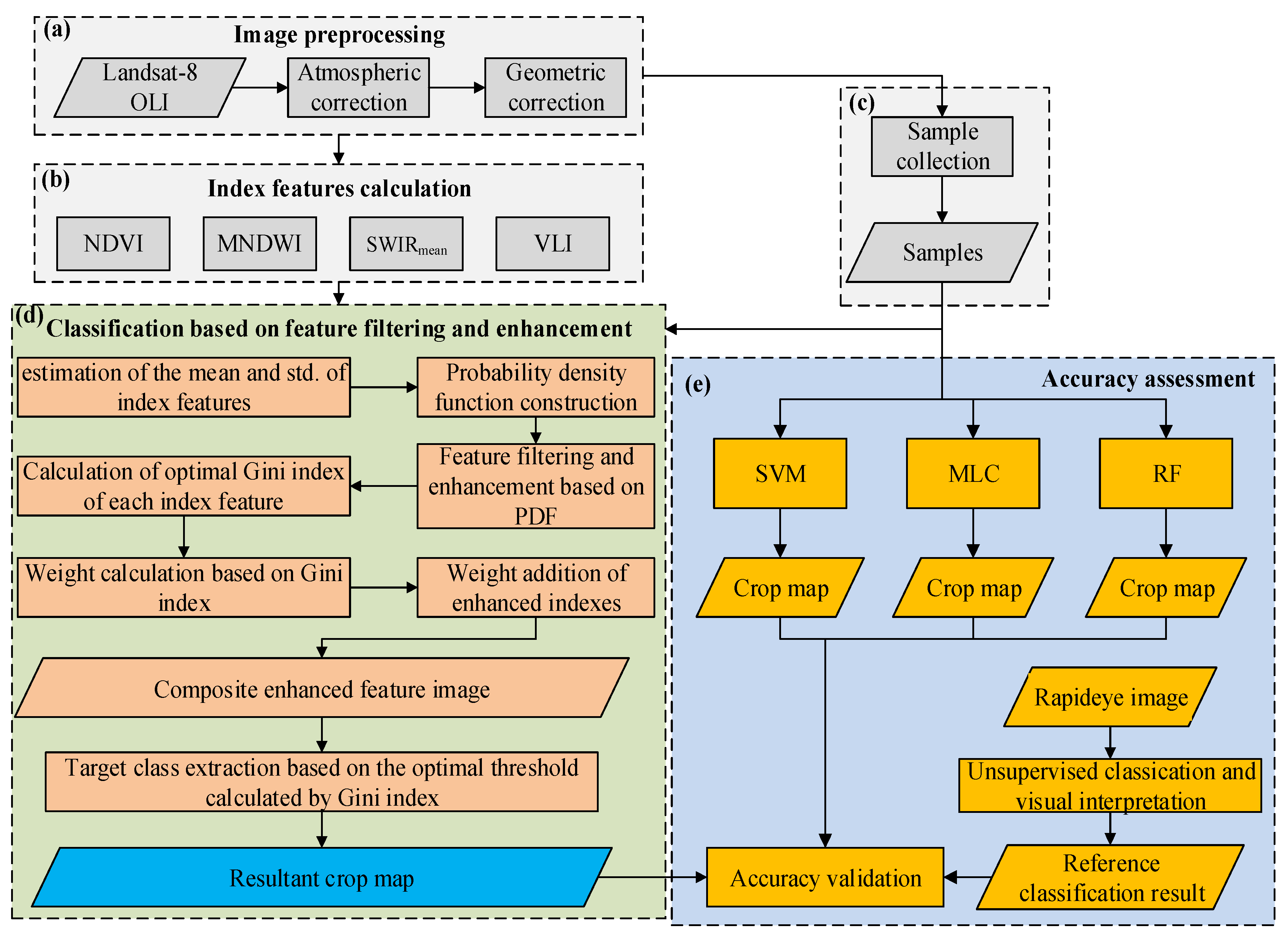
Figure 2 shows the flow chart of FFE-based crop classification, which includes the following steps:
(1) Image pre-processing, including atmospheric correction, geometric correction (Figure 2a), and generation of the indices including NDVI, MNDWI, NDSI, and VLI (Figure 2b);
(2) Ground sampling for the parcels including maize, soybean, water, built-up area, bare land, and grassland. Woodland, water, built-up area, bare land, woodland, and grassland are merged into a common class, “others”, as the main classification targets are maize and soybean (Figure 2c);
(3) Calculating the probability density function (PDF) of each feature (including NDVI, MNDWI, SWIRmean, and VLI) for each class (maize, soybean, and others). The mean and standard deviation (SD) of each feature of each class are calculated previously based on the samples. Thus, the PDFs are calculated based on the normal distribution assumption and used to filter the raw index images (Figure 2d);
(4) A weighted addition method based on the Gini index, described below, is used to cumulate values of all the enhanced features and generate a single composite enhanced feature (CEF) image. Thus, based on a simple threshold calculated from the samples, the target class can be classified easily (Figure 2d);
(5) The reference image or the ground truth map is built from the visual interpretation of a RapidEye image. MLC, SVM, and RF are applied to perform crop classification and the accuracies from these classifications are compared with those of the FFE method (Figure 2e).
The major steps are elaborated in detail hereafter.
3.1. Image pre-Processing and Index Computing
Landsat image pre-processing mainly consists of radiometric calibration, atmospheric and geometric correction.
The radiometric calibration is carried out according to Equation (1):
where is spectral radiance at the sensor’s aperture in W/(m2·sr·μm), DN is the digital number of data, and Gain and Offset are obtained from the metadata of Landsat imagery in units of W/(m2·sr·μm). Atmospheric correction is conducted using the fast line-of-sight atmospheric analysis of spectral hypercubes (FLAASH) module in ENVI software [33]. Geometric correction is carried out to ensure that the positioning accuracy between Landsat images and RapidEye image reaches the sub-pixel level.
3.2. Sampling
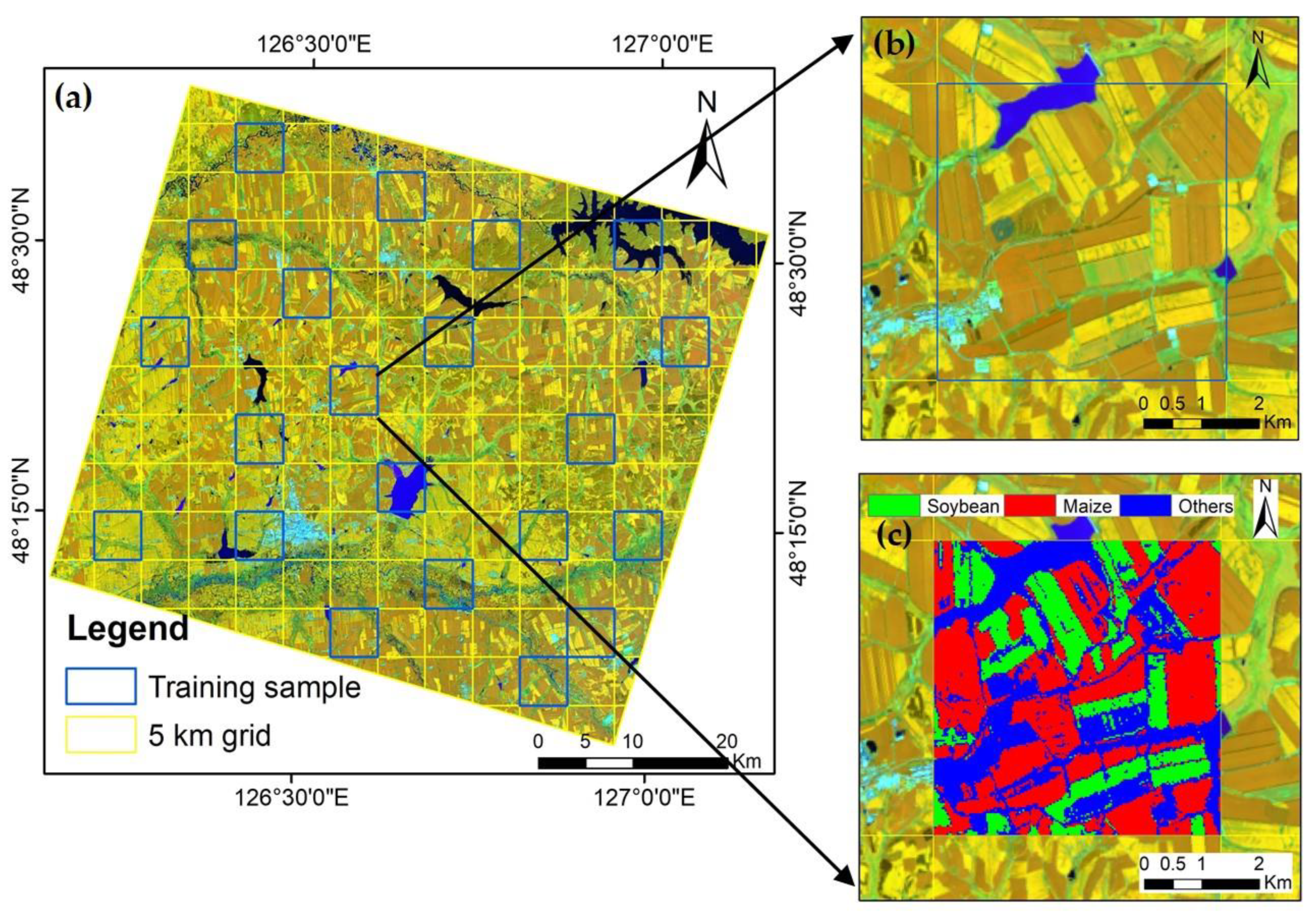
The entire study area is divided into a regular grid of 5 km×5 km consisting of 164 blocks, among which 110 are entire blocks. Then, simple random sampling is used to select 21 sample blocks from the set of these 110 blocks. Visual interpretation is applied to obtain the classification result of each block (Figure 3).
Within the total area of 525.0 km2 for these 21 blocks, maize occupies 149.7 km2 and soybean takes up 156.6 km2. Forest, grassland, road, water, built-up area, etc., are merged into the class “others”, which represents 218.7 km2 of the area. In terms of percentage, the classes maize, soybean, and others, respectively, account for 28.5%, 29.8%. and 41.7% of the total area.
3.3. Feature Filtering and Enhancement Based on Probability Density Function
Based on the samples, the mean and standard deviation of each index of each class are estimated. Thus, based on the assumption of normal distribution, the probability density function (PDF) can be calculated:
where is the PDF of index value, μ is the mean value, and σ is the standard deviation. Then, the PDF can be calculated as follows:
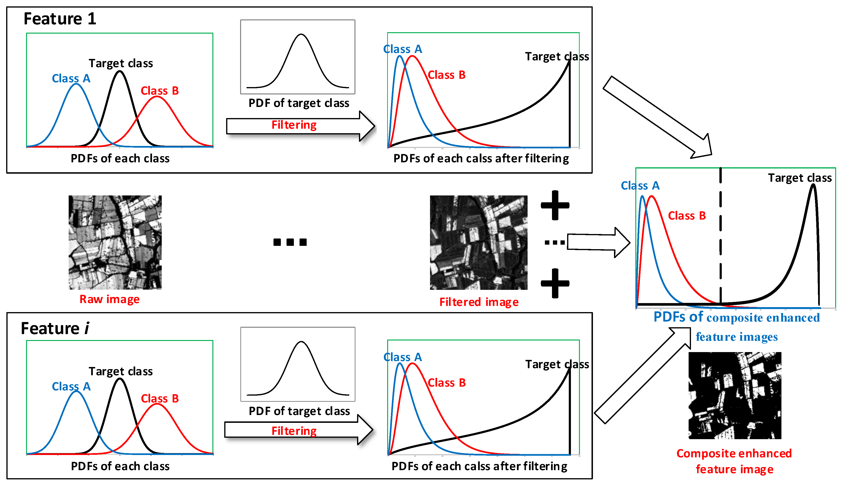
After obtaining the PDFs of all classes (including soybean, maize, and others) for all indices (including NDVI, MNDWI, SWIRmean, and VLI), the PDFs of the target class are used to filter the raw index images based on Equation (7). Thus, the value of the target class in the filtered image can be calculated as follows:
where is the index value in the raw image, and are the mean and standard deviation of the target class in the raw image, and is the filtered value in the filtered image.
Due to the characteristics of the Gauss filter (Equation (7)), a pixel with a value closer to will have a higher value after filtering:
where is the index value of the background classes, and is the filtered value of background classes.
Under the assumption of normal distribution, the values of pixels of the target class () are mostly (about 95.4%) concentrated in the range of ± 2; thus, they will usually have higher values than other classes with different PDFs (Figure 4).
3.4. Weighted Addition of Index Features and Crop Classification
Different vegetation index values of a target class in the filtered images are linearly combined into a single image. As some vegetation coefficients are more important than others in crop discrimination, the coefficients or the weights for each variable (index) are determined using the Gini index, which is widely used in some decision tree classification methods, such as the classification and regression tree (CART) and random forest (RF) [36,37]. The Gini index is an index for estimating the uncertainty of data; the lower the Gini index, the higher the data purity. If one image is perfectly classified, its Gini index would be zero. The Gini index is calculated by subtracting the sum of the squared probabilities of each class from one [38]. Suppose that there are m classes in image D, in which the probability of occurrence of the class i is pi, then the Gini index of D is:
When image D is segmented into two parts (D1 and D2) according to a certain feature A, then the Gini index of the segmented image D is:
where QTY refers to the quantity of data in a certain dataset. Gini(D1) and Gini(D2) can be determined according to Equation (10).
Here, each filtered image is segmented into two parts based on a threshold: the target class and other classes. As described in Section 3.3, the feature or index value of the target class in the filtered image is usually higher than that of other classes. A pixel with an index value higher than the threshold will be classified into target class; otherwise, it will be classified into other classes. An automatic approach is employed in this study to calculate the optimal threshold which will lead to an optimal classification (lowest Gini index). Samples collected in Section 3.2 are used to calculate the Gini index of the classification.
First, the maximum value and minimum value of the filter image are calculated, then 100 thresholds for Ti (i = 1, 2, …, 100) are obtained based on the following formula:
Then, each threshold is used to segment the image into two parts, and the Gini index of each segmentation will be calculated based on Equation (11). The threshold with the lowest Gini index will be selected as the optimal threshold, as it can generate the most accurate classification result. The lowest Gini index of the filtered image will then be used to calculate the weight of the filtered index image. Suppose the number of index images is n; then, the weight of each filtered image can be calculated as follows:
where Wi is the weight of filtered image i, and Ginii is the lowest Gini index of filtered image i.
All filtered images multiplied by their weights are combined to obtain a single composite enhanced feature (CEF) image:
where Ii is the index image i.
After obtaining the CEF image, an optimal threshold will be applied to classify the image and obtain the final classification result. The optimal threshold can be calculated automatically in the same way as the selection of the optimal threshold of each filtered image, as described above. A series of thresholds will be generated based on Equation (12) and used to classify the CEF image, and the threshold with the lowest Gini index will be selected as the optimal threshold.
3.5. Accuracy Assessment
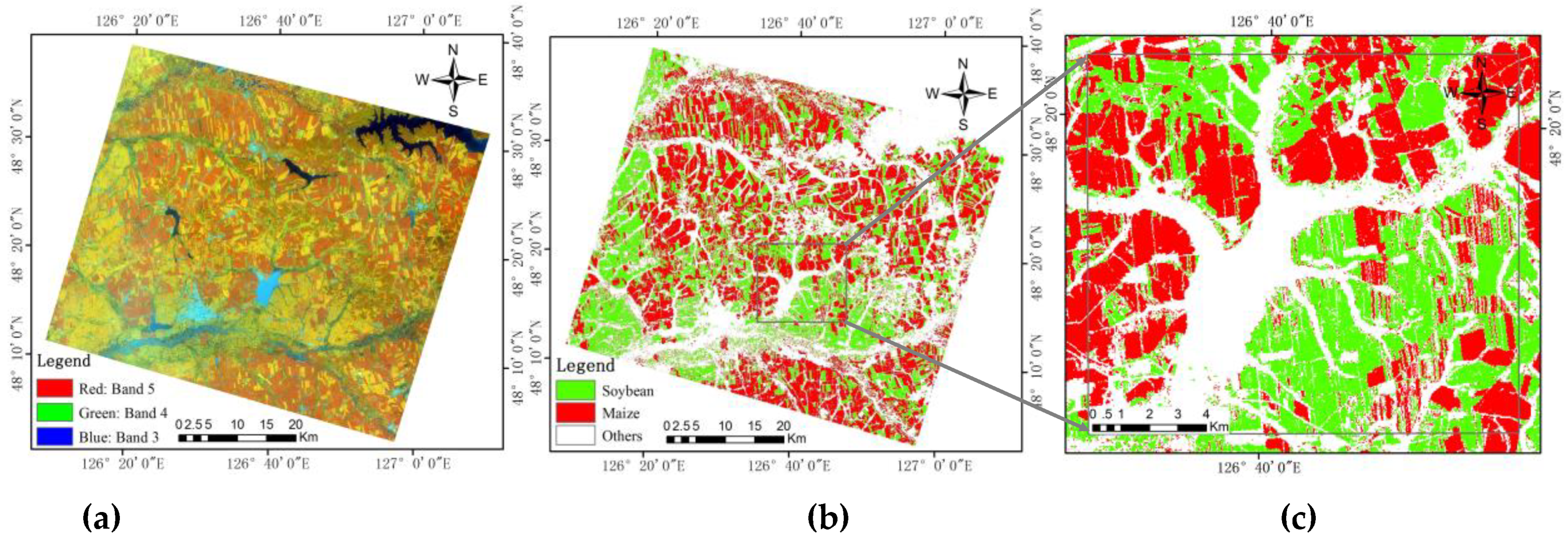
The classification of a RapidEye image registered on July 27, 2014 is used as the reference or ground truth map for accuracy assessment (Figure 5). Unsupervised Iterative Self-Organizing Data Analysis (ISODATA) classification [39,40] is applied, followed by a visual interpretation to further reclassify the raw classes into soybean, maize and others. Accuracy assessment is made based on the confusion matrix, including overall accuracy (OA), producer’s accuracy (PA), user’s accuracy (UA) metrics [41,42], and kappa coefficient [43].
In order to evidence the superior capability of discrimination for the FFE method in the study case, the maximum likelihood classification [44,45,46], support vector machine [18,47] and random forest [36] are applied for Landsat image classification using the same sample dataset as in the application of the FFE method.
4. Results and Discussion
4.1. Vegetation Index Calculation
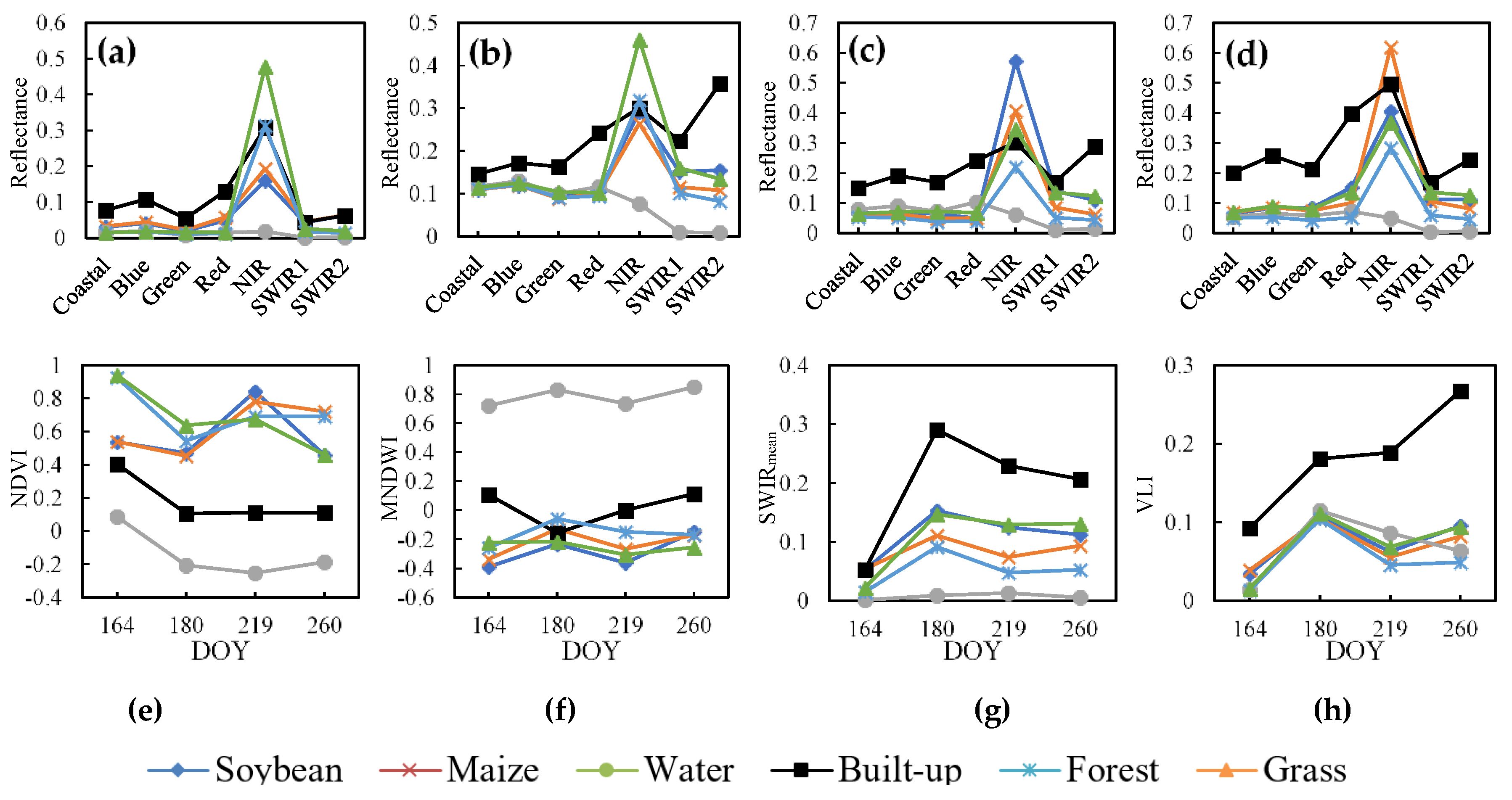
The spectral curves of the main classes are shown in Figure 6. Grassland and forest have higher NIR values, and thus higher NDVI values, at the early growing stage (DOY 164) (Figure 6a,e). The NIR values (thus, the NDVIs for the values of red band of maize and soybean are similar) for the class maize are usually lower than those for soybean on DOY 219 (Figure 6c,e), and are higher than those of soybean on DOY 260 (Figure 6d,e). Shortwave infrared (SWIR) is another critical band for identifying maize and soybean [48,49]. The SWIRmean of soybean is generally higher than that of maize in the whole growing season (Figure 6g). The MNDWI of water is much higher than those of other classes (Figure 6f). VLI represents the brightness of all classes in visible spectral bands, which will be useful for distinguishing between high brightness classes (e.g., built-up area) and low brightness classes (e.g., vegetation and water) (Figure 6h). Moreover, the NDVI values of soybean and maize decreased from day 164 to day 180. This is mainly due to there being some mist in the image of DOY 180, which resulted in the increase of the reflectance of visible bands (including red band), and then led to the decrease of NDVI on day 180. Besides this, the significant increase of the NDVI values of soybean and maize on day 219 was mainly due to the vigorous growth of crops.
4.2. Distribution and probability Density Function (PDF) for three target classes
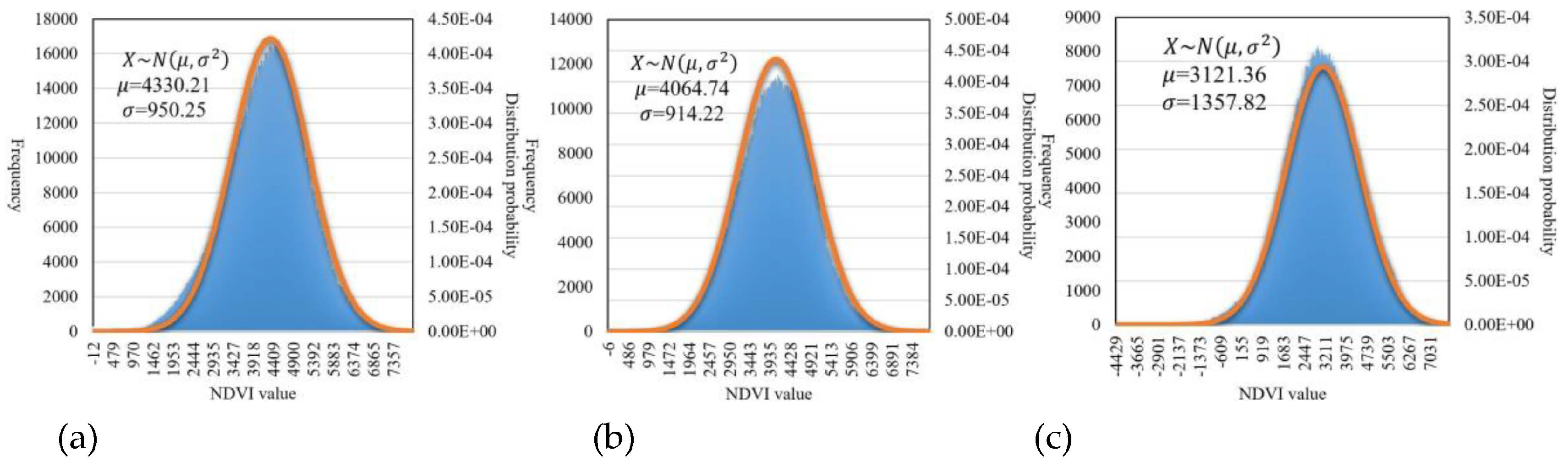
After obtaining the indices, the PDFs of each index and each class are calculated by Equation (7). Figure 7 shows the PDFs of the NDVI of maize, soybean and others on DOY 180. This indicates that the distribution of NDVI values displays the profile of a normal distribution function. The PDFs will be used to filter the raw index images.
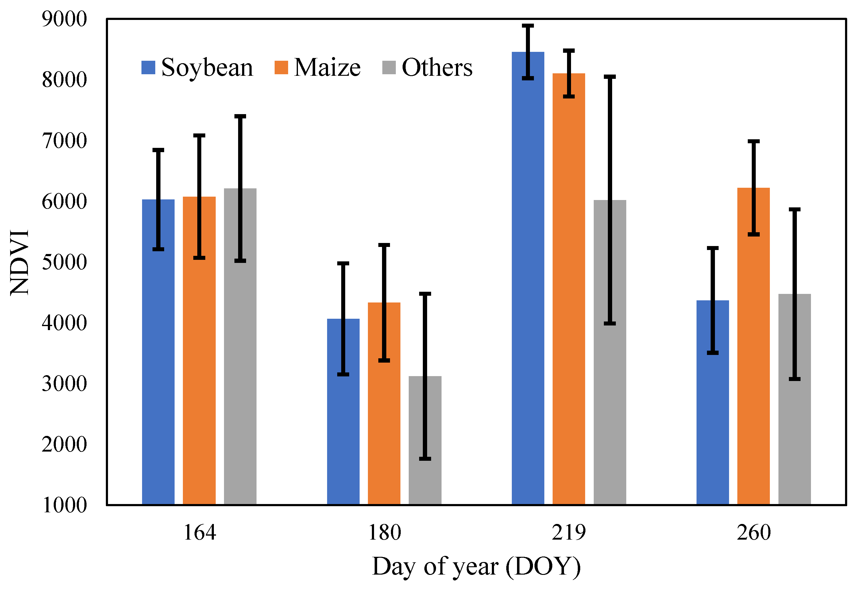
Figure 8 illustrates the mean and standard deviations of the NDVI of soybean, maize and others at different growing stages. In Figure 8, the error bar is ±1σ. This shows that the mean NDVIs of soybean and maize are close to each other on DOY 164, 180, and 219, while they show a significant difference on DOY 260. The mean values of crops (soybean and maize) and others are significantly different on DOY 180 and 219.
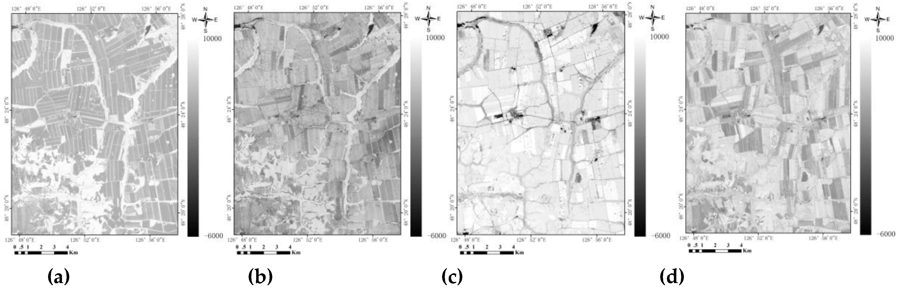
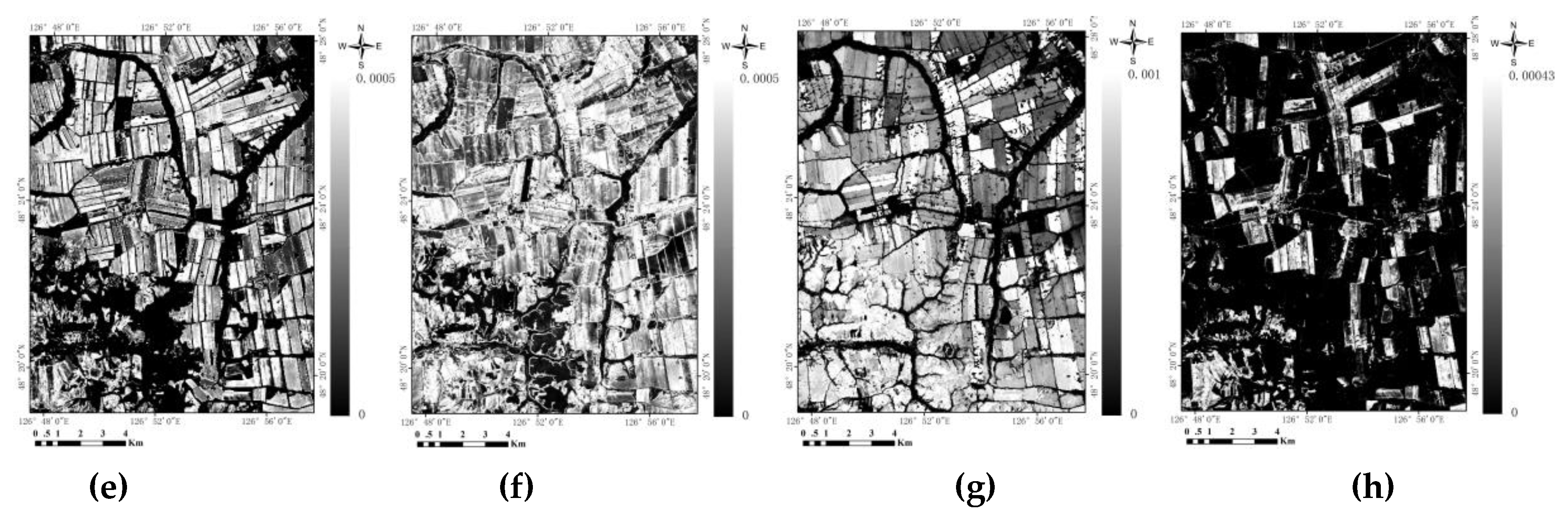
Due to the characteristics of Gauss filtering, the target class pixels will have amplified values in the filtered images. Figure 9 shows the raw NDVI images and the corresponding filtered images of soybean at different stages. It is obvious that the difference between soybean and other classes is significantly expanded after filtering.
4.3. FFE-Based Classification
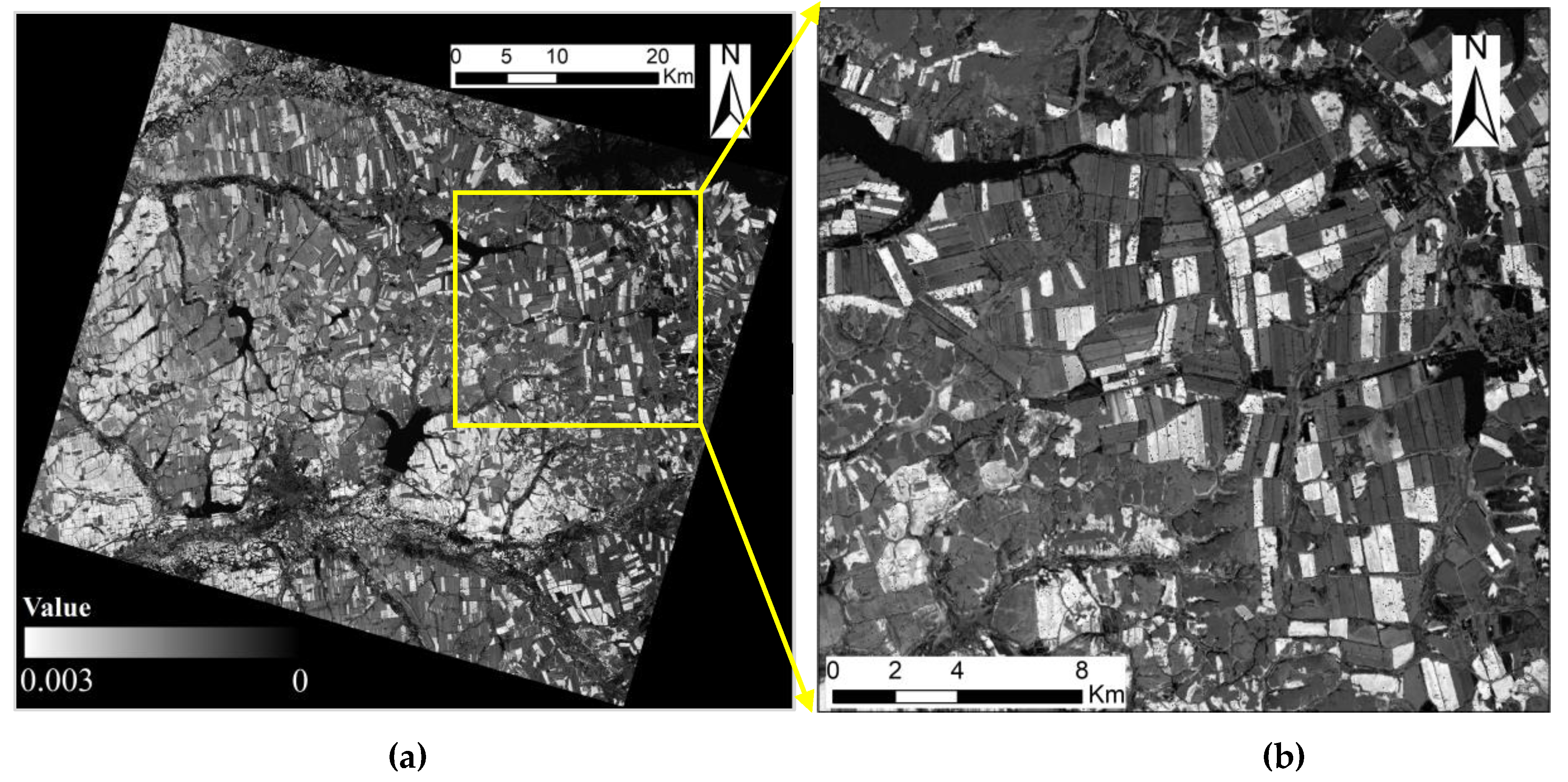
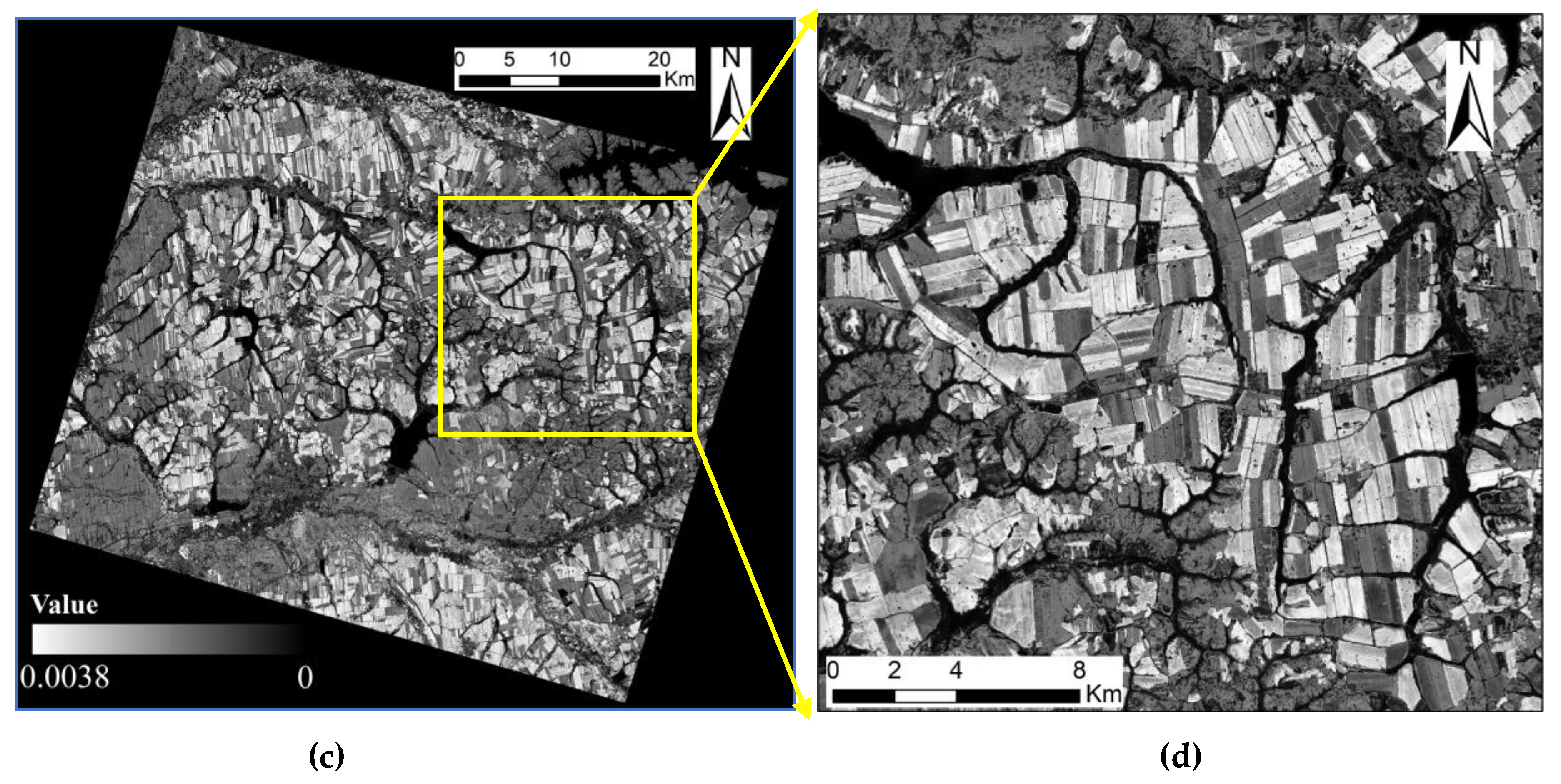
The CEF images of soybean and maize are shown in Figure 10. This indicates that the FFE method can significantly enlarge the difference between the target class and background classes, which makes it easy to extract the target class based on a single threshold. There are two reasons why the FFE method could enlarge the feature difference of different classes: firstly, the PDF-based filter makes the feature values of the target class much higher, in that they are concentrated around the mean value which has the highest PDF value; secondly, the weighted addition of filtered features makes this high value even higher, because the target class always has the highest values in each image of the filtered feature.
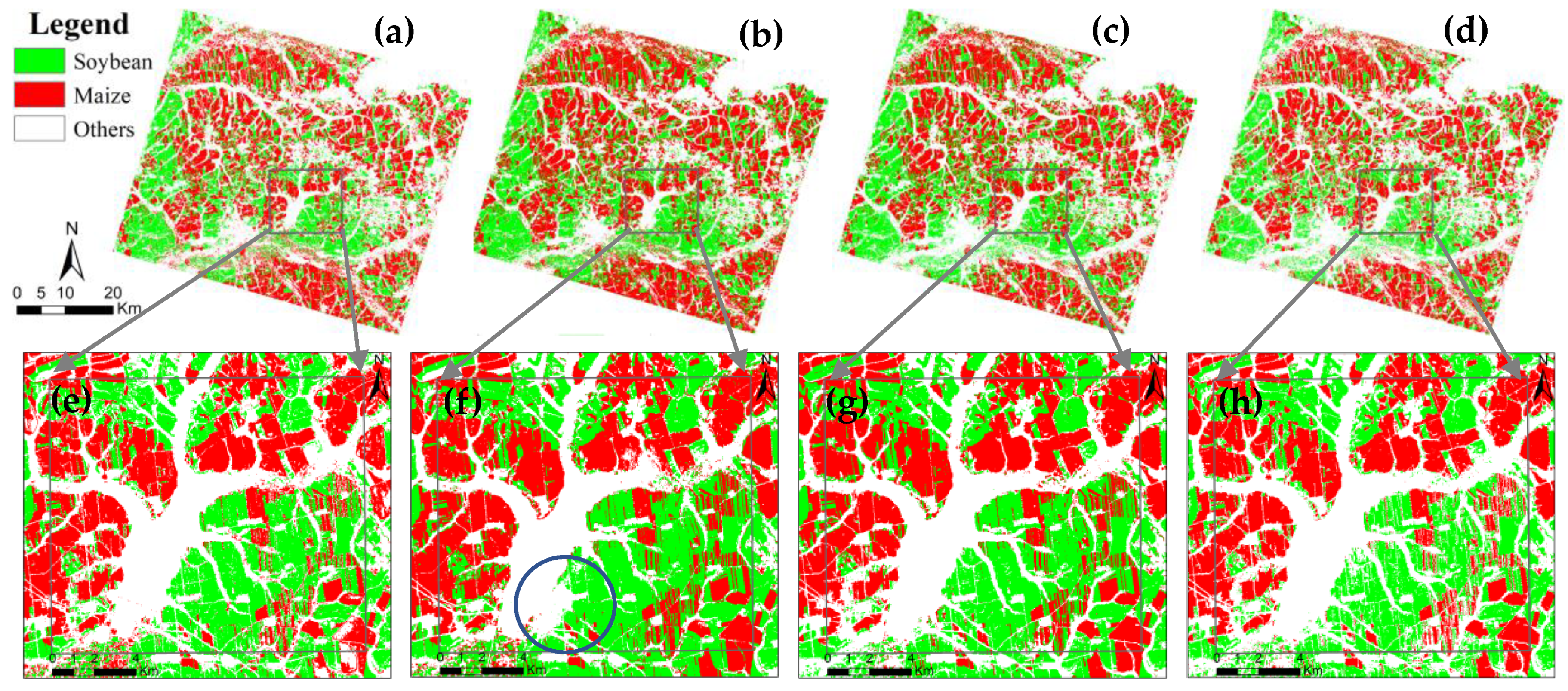
Figure 11 shows that the classification results of FFE, MLC, SVM, and RF methods, which are very comparable; however, there are some omissions in the MLC result as shown in the circular area of Figure 11b.
Figure 12 shows the classification accuracies of the FFE, MLC, SVM and RF methods. The result shows that the overall accuracy of the FFE method (0.902) is much higher than that of the MLC method, while it is similar to those of SVM (0.899) and RF (0.912).
Moreover, the FFE and RF methods obtain much higher UAs for soybean (0.910 and 0.926, respectively) and maize (0.911 and 0.943, respectively) than those of MLC (0.729 for soybean and 0.802 for soybean) and SVM (0.864 for soybean and 0.811 for maize). However, SVM obtains the highest PAs for soybean (0.956) and maize (0.988), and the highest UA for ‘other’ (0.983). This indicates that SVM has misclassified more pixels of the ‘other’ class into maize and soybean than other way.
The results show that the FFE method is appropriate for an accurate mapping of maize and soybean in the study area, by higher overall accuracy and Kappa coefficient compared to the MLC and SVM methods, while having similar accuracy to RF.
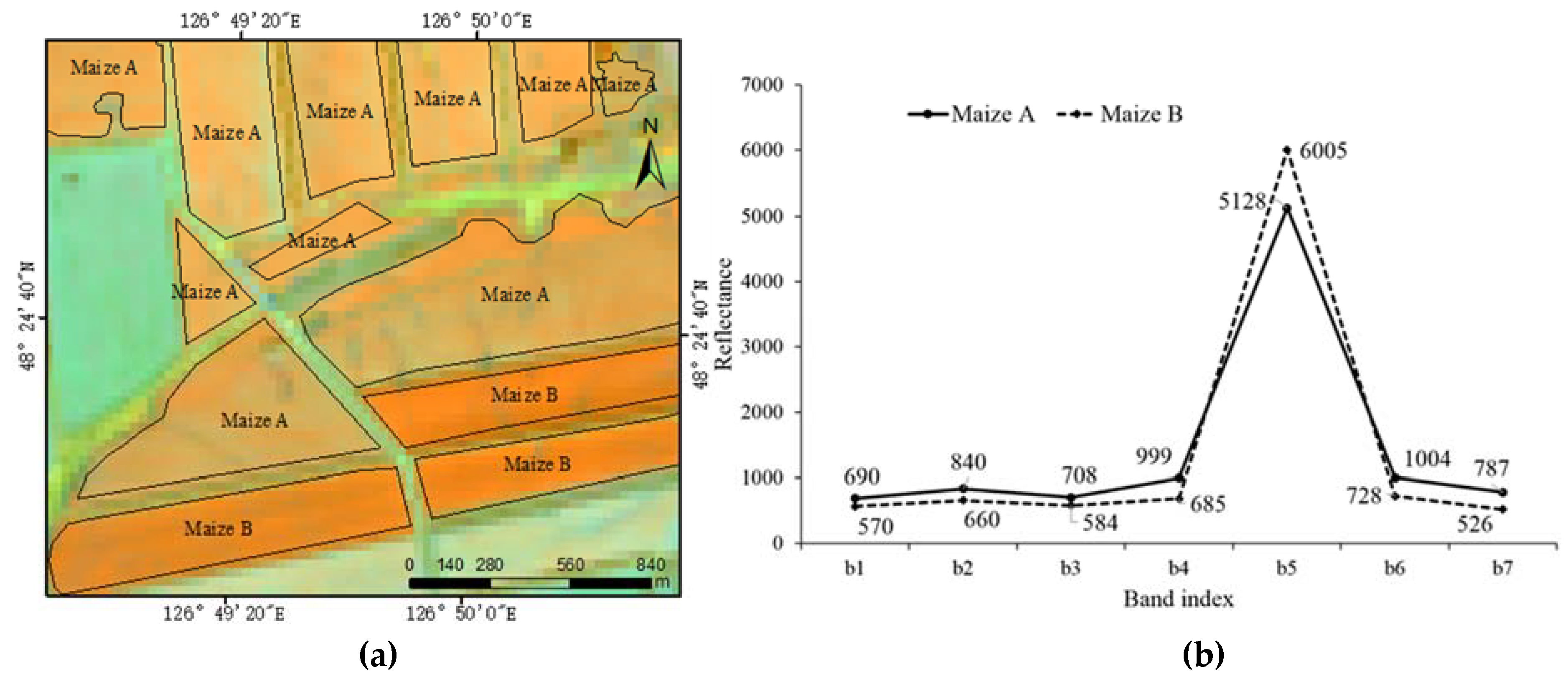
The misclassification of the FFE method has been analyzed and indicates that those errors mainly appear on the fringe of the farmland parcels because the OLI images have a lower resolution than the RapidEye image, which leads to a mixed pixel phenomenon. Other classification errors are attributed to the different spectral responses from different subclasses or varieties of a crop. For example, two sub-classes of maize (marked as maize A and maize B) can be founded in the study area as shown in Figure 13a. However, maize B is misclassified into the class ‘others’ by the FFE method. In this case, the spectral values of maize B are different from those of maize A (see Figure 13b) due to a sowing date delay. Therefore, after the Gaussian filtering of images, the value of maize B is always lower than maize A, and this leads to the omission of maize B. When this phenomenon is significant, it is necessary to divide the same crop with different sowing dates or different genotypes into different classes during the sampling phase.
4.4. The Impact of Sample Size on Probability Density Function
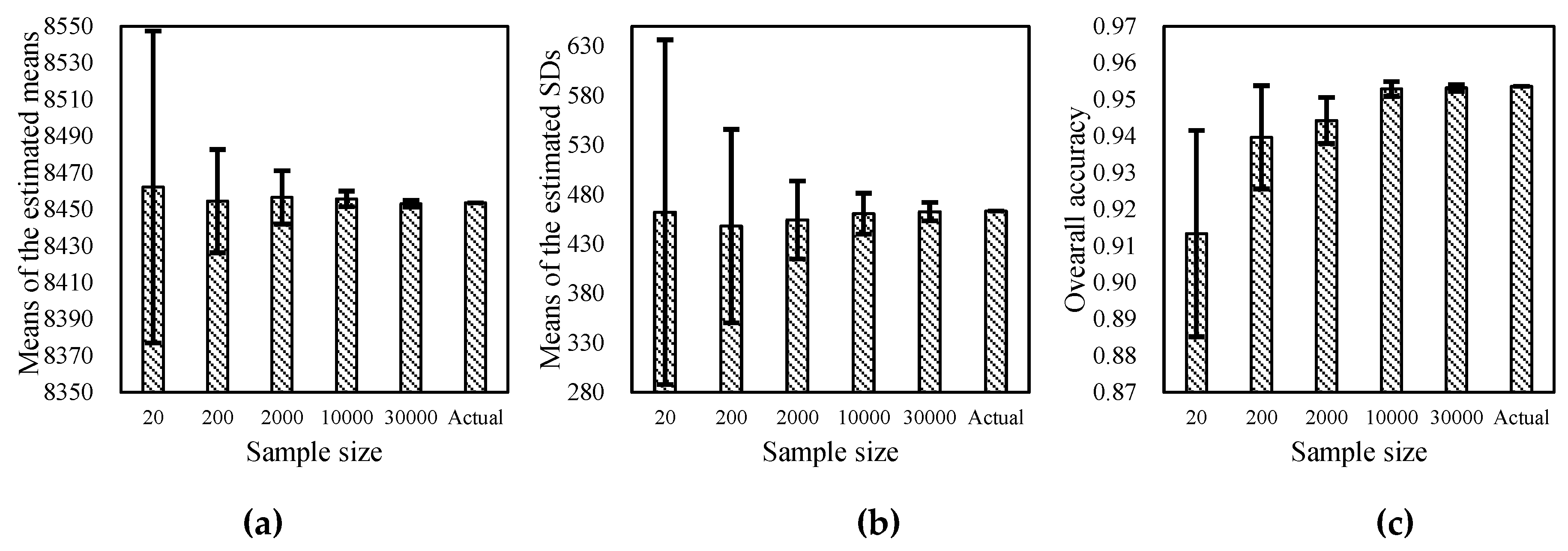
The sample size has a direct influence on the accuracy of the estimation of the mean and standard deviation of the feature values of one class. When the sample size is large enough, the mean value of the samples tends to be close to the actual mean value. However, a large sample size means large operational resources. In order to evaluate the impact of sample size on mean and standard deviation (SD) estimation, five sample datasets are randomly selected from the reference classification data. The sizes of these five sample datasets are 20, 200, 2000, 10,000, and 30,000 pixels, respectively. The mean and SD values of each sample dataset are calculated based on the Landsat NDVI image of DOY 219. All of the five sample datasets are randomly selected 10 times, and the mean and SD of the mean and SD values are calculated. Furthermore, the actual mean and SD of soybean are also calculated based on all soybean pixels of the reference classification data. Finally, the classification accuracy of soybean is evaluated based on the calculated PDFs. The results are shown in Figure 14. They indicate that the estimated mean values are very close to the actual value, even when the sample size is very small. The standard deviation of the estimated mean value is also very small, which indicates the stability of the estimated mean value. The result shows that the impact of sample size on mean value estimation is limited. However, regarding the estimated SD values, the conclusion is different; Figure 14b shows that when the sample size is small, the estimated SD could be greatly different to the actual value. Although the means of the SDs are close to the actual SD, the standard deviation of SDs tend to increase when the sample size decreases. When the sample size is 20, the standard deviation of SD is up to 174, which is quite large when compared with the actual SD (463), and may lead to inaccurate PDF calculation and a low classification accuracy (Figure 14c). Finally, with the increase of the sample size, the classification accuracy is gradually improved. The results indicates that it is necessary to obtain a sufficiently large size (e.g., >2000) of sample to ensure the accuracy of the mean and SD estimation.
4.5. Calculate PDF Based on the Bookup Table (LUT) Method Instead of Normal Distribution Function
If the data do not conform to a normal distribution, the normal distribution function can be replaced using a lookup table method. Thus, Equation (7) will be replaced by a LUT obtained by sample data statistics. LUT records the index values of the target class and their corresponding proportion to the total number of pixels of target class. Other steps remain the same as the normal distribution function-based classification method. In order to evaluate the effectiveness of the LUT method, the PDF, calculated by a lookup table, is used to perform the crop classification of the study area based on the same samples. The classification accuracy is illustrated in Figure 12; it indicates that the accuracy of classification is not remarkably different from before. There are two possible reasons for this: one is that the probability density function in this study is almost normal, which limits the role of the lookup table; another is that the PDFs calculated by LUT may also deviate from the actual PDFs. Moreover, the LUT may not be able to represent the actual PDF when the sample size is small.
5. Conclusions
This paper proposes an approach of feature enhancement for crop classification using probability density function filtering. This led to a better extraction of the cropping areas for maize and soybean in the study region. This improvement is evidenced by a better classification accuracy compared to the MLC and SVM methods. The proposed method also achieves a similar accuracy to the RF method in the study area. Moreover, this method can be considered as a non-parametric method, as few parameters need to be defined by users except sample selection, which makes it a user-friendly method for classification. Each step of the FFE method is visible and logical to the user, which makes it much easier for users to understand. The importance of each index can be calculated based on the weight of each filtered image. Simple visual methods can also be used to understand the importance of each index for crop classification based on the filtered images (Figure 9). This will be useful in the selection of important indices and reduce redundant features in crop classification based on multi-temporal images.
This paper also discusses the impact of sample size on the estimation of PDF and classification accuracy. The result shows the estimated mean values of index feature for both crops are close to the actual value, even when the sample size is small. However, the standard deviation of SD is significant when the sample size is small, which may lead to an inaccurately estimated SD value. Moreover, the estimated mean and SD tend to be stable when the sample size is, for example, above 2000 in the FFE method. The classification accuracy will also increase with the increase of sample size.
When the feature values of crops are not normally distributed, a LUT-based PDF calculated method could be employed to filter the features in the FFE method. However, the sample size has to be sufficiently large in order to have an accurate probability density function of feature distribution.
For the classes with binomial or multi-nominal spectral distribution, they have to be further categorized into sub-classes according to their spectral features, rather than being treated as one class.
It is worthwhile to note that the accuracy of the FFE method may be decreased when the PDFs of different crops are highly similar. Moreover, because the principle of this method is relatively simple, when the probability density function of the target class is too complex, it may not be possible to achieve higher accuracy.
Finally, more works are needed to evaluate the feasibility of the FFE method for different crops and in different areas. We expect that this method could constitute a simple, easy and accurate way to improve crop classification in an operational context.
Author Contributions
Conceptualization, L.W., J.L. and L.Y.; Methodology, L.W.; Software, L.Y.; Validation, J.L.; Formal Analysis, L.W., L.Y. and J.L.; Investigation, L.W. and J.L.; Resources, L.W.; Data Curation, L.W. and L.Y.; Writing-Original Draft Preparation, L.W., L.Y.; Writing-Review & Editing, L.W., Q.D., J.G. and J.L.; Visualization, J.G.; Supervision, Q.D.; Project Administration, L.W. and J.L.; Funding Acquisition, L.W. and J.L.
Funding
This research was funded by the Major Project for High-Resolution Earth Observation in China grant number 09-Y20A05-9001-17/18 and the APC was funded by the Major Project for High-Resolution Earth Observation in China grant number 09-Y20A05-9001-17/18.
Acknowledgments
This study was supported by the Major Project for High-Resolution Earth Observation in China (grant no. 09-Y20A05-9001-17/18). We thank Fugang Yang and Baomin Yao of the Institute of Agricultural Resources and Regional Planning, Chinese Academy of Agricultural Sciences, for their help in ground data collection. We also thank the editors and anonymous reviewers for their constructive comments and advice.
Conflicts of Interest
The authors declare no conflict of interest.
References
- Boryan, C.; Yang, Z.; Mueller, R.; Craig, M. Monitoring US agriculture: The US Department of Agriculture, National Agricultural Statistics Service, Cropland Data Layer Program. Geocarto Int. 2011, 26, 341–358. [Google Scholar] [CrossRef]
- Boryan, C.G.; Yang, Z. A new land cover classification based stratification method for area sampling frame construction. In Proceedings of the International Conference on Agro-Geoinformatics, Shanghai, China, 2–4 August 2012; pp. 639–644. [Google Scholar]
- Gallego, J.; Bamps, C. Using CORINE land cover and the point survey LUCAS for area estimation. Int. J. Appl. Earth Obs. 2008, 10, 467–475. [Google Scholar] [CrossRef]
- Shen, K.; He, H.; Meng, H.; Guannan, S. Review on Spatial Sampling Survey in Crop Area Estimation. Chin. J. Agric. Resour. Reg. Plan. 2012, 33, 11–16. [Google Scholar]
- Tatsumi, K.; Yamashiki, Y.; Morales Morante, A.K.; Ramos Fernandez, L.; Apaclla Nalvarte, R. Pixel-based crop classification in Peru from Landsat 7 ETM+ images using a Random Forest model. J. Agric. Meteorol. 2016, 72, 1–11. [Google Scholar] [CrossRef] [Green Version]
- Zhou, T.; Pan, J.; Zhang, P.; Wei, S.; Han, T. Mapping Winter Wheat with Multi-Temporal SAR and Optical Images in an Urban Agricultural Region. Sensors 2017, 17, 1210. [Google Scholar] [CrossRef]
- Dong, J.; Xiao, X.; Kou, W.; Qin, Y.; Zhang, G.; Li, L.; Jin, C.; Zhou, Y.; Wang, J.; Biradar, C. Tracking the dynamics of paddy rice planting area in 1986–2010 through time series Landsat images and phenology-based algorithms. Remote Sens. Environ. 2015, 160, 99–113. [Google Scholar] [CrossRef] [Green Version]
- Kussul, N.; Lemoine, G.; Gallego, F.J.; Skakun, S.V. Parcel-Based Crop Classification in Ukraine Using Landsat-8 Data and Sentinel-1A Data. IEEE J. Sel. Top. Appl. Earth Obs. Remote Sens. 2017, 9, 2500–2508. [Google Scholar] [CrossRef]
- Veloso, A.; Mermoz, S.; Bouvet, A.; Le Toan, T.; Planells, M.; Dejoux, J.; Ceschia, E. Understanding the temporal behavior of crops using Sentinel-1 and Sentinel-2-like data for agricultural applications. Remote Sens. Environ. 2017, 199, 415–426. [Google Scholar] [CrossRef]
- Wu, M.; Zhang, X.; Huang, W.; Niu, Z.; Wang, C.; Li, W.; Hao, P. Reconstruction of daily 30 m data from HJ CCD, GF-1 WFV, Landsat, and MODIS data for crop monitoring. Remote Sens. 2015, 7, 16293–16314. [Google Scholar] [CrossRef]
- Immitzer, M.; Vuolo, F.; Atzberger, C. First Experience with Sentinel-2 Data for Crop and Tree Species Classifications in Central Europe. Remote Sens. 2016, 8, 166. [Google Scholar] [CrossRef]
- Siachalou, S.; Mallinis, G.; Tsakiri-Strati, M. A hidden Markov models approach for crop classification: Linking crop phenology to time series of multi-sensor remote sensing data. Remote Sens. 2015, 7, 3633–3650. [Google Scholar] [CrossRef]
- Gaertner, J.; Genovese, V.B.; Potter, C.; Sewake, K.; Manoukis, N.C. Vegetation classification of Coffea on Hawaii Island using WorldView-2 satellite imagery. J. Appl. Remote Sens. 2017, 11, 046005. [Google Scholar] [CrossRef]
- Van Tricht, K.; Gobin, A.; Gilliams, S.; Piccard, I. Synergistic use of radar Sentinel-1 and optical Sentinel-2 imagery for crop mapping: A case study for Belgium. Remote Sens. 2018, 10, 1642. [Google Scholar] [CrossRef]
- Wessel, M.; Brandmeier, M.; Tiede, D. Evaluation of Different Machine Learning Algorithms for Scalable Classification of Tree Types and Tree Species Based on Sentinel-2 Data. Remote Sens. 2018, 10, 1419. [Google Scholar] [CrossRef]
- Li, Q.; Wang, C.; Zhang, B.; Lu, L. Object-based crop classification with Landsat-MODIS enhanced time-series data. Remote Sens. 2015, 7, 16091–16107. [Google Scholar] [CrossRef]
- Chi, M.; Rui, F.; Bruzzone, L. Classification of hyperspectral remote-sensing data with primal SVM for small-sized training dataset problem. Adv. Space Res. 2008, 41, 1793–1799. [Google Scholar] [CrossRef]
- Chang, C.; Lin, C. LIBSVM: A library for support vector machines. ACM Trans. Intell. Syst. Technol. (Tist) 2011, 2, 27. [Google Scholar] [CrossRef]
- Tan, C.P.; Hong, T.E.; Chuah, H.T. Agricultural crop-type classification of multi-polarization SAR images using a hybrid entropy decomposition and support vector machine technique. Int. J. Remote Sens. 2011, 32, 7057–7071. [Google Scholar] [CrossRef]
- Rodriguez-Galiano, V.F.; Ghimire, B.; Rogan, J.; Chica-Olmo, M.; Rigol-Sanchez, J.P. An assessment of the effectiveness of a random forest classifier for land-cover classification. ISPRS J. Photogramm. Remote Sens. 2012, 67, 93–104. [Google Scholar] [CrossRef]
- Ok, A.O.; Akar, O.; Gungor, O. Evaluation of random forest method for agricultural crop classification. Eur. J. Remote Sens. 2012, 45, 421–432. [Google Scholar] [CrossRef]
- Lebourgeois, V.; Dupuy, S.; Vintrou, É.; Ameline, M.; Butler, S.; Bégué, A. A Combined Random Forest and OBIA Classification Scheme for Mapping Smallholder Agriculture at Different Nomenclature Levels Using Multisource Data (Simulated Sentinel-2 Time Series, VHRS and DEM). Remote Sens. 2017, 9, 259. [Google Scholar] [CrossRef]
- Holloway, J.; Mengersen, K. Statistical Machine Learning Methods and Remote Sensing for Sustainable Development Goals: A Review. Remote Sens. 2018, 10, 1365. [Google Scholar] [CrossRef]
- Tang, K.; Zhu, W.; Zhan, P.; Ding, S. An Identification Method for Spring Maize in Northeast China Based on Spectral and Phenological Features. Remote Sens. 2018, 10, 193. [Google Scholar] [CrossRef]
- Nagaraja, A.; Sahoo, R.N.; Usha, K.; Gupta, V.K. Estimation of mango growing areas using remote sensing. Indian J. Hortic. 2017, 74, 184–188. [Google Scholar] [CrossRef]
- Ouyang, L.; Mao, D.; Wang, Z.; Li, H.; Man, W.; Jia, M.; Liu, M.; Zhang, M.; Liu, H. Analysis crops planting structure and yield based on GF-1 and Landsat8 OLI images. Trans. Chin. Soc. Agric. Eng. 2017, 33, 147–156. [Google Scholar]
- Wang, L.; Chen, X.; Qi, L.; Wu, D.; Zhang, T. Phenology Extraction of Winter Wheat Based on Different time Series Vegetation Index Reconstructing Methods in Jiangsu Province. Sci. Technol. Eng. 2017, 17, 192–199. [Google Scholar]
- Wardlow, B.D.; Egbert, S.L. A comparison of MODIS 250-m EVI and NDVI data for crop mapping: A case study for southwest Kansas. Int. J. Remote Sens. 2010, 31, 805–830. [Google Scholar] [CrossRef]
- Mansaray, L.; Huang, W.; Zhang, D.; Huang, J.; Li, J. Mapping Rice Fields in Urban Shanghai, Southeast China, Using Sentinel-1A and Landsat 8 Datasets. Remote Sens. 2017, 9, 257. [Google Scholar] [CrossRef]
- Li, J.; Xi, B.; Li, Y.; Du, Q.; Wang, K. Hyperspectral Classification Based on Texture Feature Enhancement and Deep Belief Networks. Remote Sens. 2018, 10, 396. [Google Scholar] [CrossRef]
- Zhang, J.; Yang, J.; Zhao, Z.; Li, H.; Zhang, Y. Block-regression based fusion of optical and SAR imagery for feature enhancement. Int. J. Remote Sens. 2010, 31, 2325–2345. [Google Scholar] [CrossRef]
- Heihe Statistical Bureau Heihe Social and Economic Statistics Yearbook; China Statistical Publishing House: Beijing, China, 2014.
- Harris Geospatial Solutions The Environment for Visualizing Images (ENVI), 5.3; Interlocken Crescent: Broomfield, CO, USA, 2015.
- Rouse, J.W.J.; Haas, R.H.; Schell, J.A.; Deering, D.W. Monitoring Vegetation Systems in the Great Plains with Erts. NASA Spec. Publ. 1974, 351, 309. [Google Scholar]
- Xu, H. Modification of normalised difference water index (NDWI) to enhance open water features in remotely sensed imagery. Int. J. Remote Sens. 2006, 27, 3025–3033. [Google Scholar] [CrossRef]
- Breiman, L. Random Forests. Mach. Learn. 2001, 45, 5–32. [Google Scholar] [CrossRef] [Green Version]
- Breiman, L.; Friedman, J.H.; Olshen, R.; Stone, C.J. Classification and Regression Trees. Encycl. Ecol. 1984, 57, 582–588. [Google Scholar]
- Decision Tree Flavors: Gini Index and Information Gain. Available online: http://www.learnbymarketing.com/481/decision-tree-flavors-gini-info-gain/ (accessed on 27 February 2016).
- Vanderzee, D.; Ehrlich, D. Sensitivity of ISODATA to changes in sampling procedures and processing parameters when applied to AVHRR time-series NDV1 data. Int. J. Remote Sens. 1995, 16, 673–686. [Google Scholar] [CrossRef]
- Zhu, C.; Lu, D.; Victoria, D.; Dutra, L. Mapping Fractional Cropland Distribution in Mato Grosso, Brazil Using Time Series MODIS Enhanced Vegetation Index and Landsat Thematic Mapper Data. Remote Sens. 2015, 8, 22. [Google Scholar] [CrossRef]
- Congalton, R.G. A review of assessing the accuracy of classification of remotely sensed data. Remote Sens. Environ. 1991, 37, 270–279. [Google Scholar] [CrossRef]
- HAY, A.M. The derivation of global estimates from a confusion matrix. Int. J. Remote Sens. 1988, 9, 1395–1398. [Google Scholar] [CrossRef]
- Cohen, J. A coefficient of agreement for nominal scales. Educ. Psychol. Meas. 1960, 20, 37–46. [Google Scholar] [CrossRef]
- Gašparović, M.; Jogun, T. The effect of fusing Sentinel-2 bands on land-cover classification. Int. J. Remote Sens. 2018, 39, 822–841. [Google Scholar] [CrossRef]
- Raju, P.V. Classification of wheat crop with multi-temporal images: Performance of maximum likelihood and artificial neural networks. Int. J. Remote Sens. 2003, 24, 4871–4890. [Google Scholar]
- Strahler, A.H. The use of prior probabilities in maximum likelihood classification of remotely sensed data. Remote Sens. Environ. 1980, 10, 135–163. [Google Scholar] [CrossRef]
- Tien Bui, D.; Shahabi, H.; Shirzadi, A.; Chapi, K.; Alizadeh, M.; Chen, W.; Mohammadi, A.; Ahmad, B.; Panahi, M.; Hong, H. Landslide detection and susceptibility mapping by AIRSAR data using support vector machine and index of entropy models in Cameron Highlands, Malaysia. Remote Sens. 2018, 10, 1527. [Google Scholar] [CrossRef]
- Cai, Y.; Guan, K.; Peng, J.; Wang, S.; Seifert, C.; Wardlow, B.; Li, Z. A high-performance and in-season classification system of field-level crop types using time-series Landsat data and a machine learning approach. Remote Sens. Environ. 2018, 210, 35–47. [Google Scholar] [CrossRef]
- Wang, L.; Jia, L.; Yang, L.; Yang, F.; Fu, C. Impact of short infrared wave band on identification accuracy of corn and soybean area. Trans. Chin. Soc. Agric. Eng. 2016, 32, 169–178. [Google Scholar]
Figure 1.
Location of study area (a) and the false color Landsat-8 image of study area (near infrared (NIR), red, green as R, G, B) (b).
Figure 1.
Location of study area (a) and the false color Landsat-8 image of study area (near infrared (NIR), red, green as R, G, B) (b).

Figure 2.
Flowchart of feature filtering and enhancement (FFE)-based crop classification. (a) Image processing; (b) Index features calculation; (c) sample collection; (d) classification based on FFE; (e) accuracy assessment. SVM: support vector machine; MLC: maximum likelihood classification; RF: random forest; NDVI: normalized difference vegetation index; MNDWI: modified normalized difference water index.

Figure 3.
Landsat image (SWIR1/NIR/Red as R/G/B) and the distribution of sample blocks (a), the enlargement of one sample block (b), and its classification (c).
Figure 3.
Landsat image (SWIR1/NIR/Red as R/G/B) and the distribution of sample blocks (a), the enlargement of one sample block (b), and its classification (c).

Figure 4.
Illustration of feature filtering and enhancement based on probability density function (PDF).
Figure 4.
Illustration of feature filtering and enhancement based on probability density function (PDF).

Figure 5.
Reference classification result based on RapidEye image. (a) RapidEye image on July 27, 2014, (b) classification result based on RapidEye image, (c) partial magnification of classification result. The reference classification result is obtained by the unsupervised Iterative Self-Organizing Data Analysis (ISODATA) and visual interpretation approaches.

Figure 6.
Spectral curves of major classes on DOY 164 (a), 180 (b), 219 (c), and 260 (d), and time series of NDVI (e), MNDWI (f), SWIRmean (g), and VLI (h).
Figure 6.
Spectral curves of major classes on DOY 164 (a), 180 (b), 219 (c), and 260 (d), and time series of NDVI (e), MNDWI (f), SWIRmean (g), and VLI (h).

Figure 7.
NDVI distributions and PDFs of soybean (a), maize (b), and others (c) on DOY 180.

Figure 8.
The mean and standard deviations of NDVI of soybean, maize, and others at different growing stage.
Figure 8.
The mean and standard deviations of NDVI of soybean, maize, and others at different growing stage.

Figure 9.
NDVI images of different stages before (a–d) and after filtering (e–h) (soybean as the target class). Figures (a) and (e) are on DOY 164, figures (b) and (f) are on DOY 180, figures (c) and (g) are on DOY 219, and figures (d) and (h) are on DOY 260.
Figure 9.
NDVI images of different stages before (a–d) and after filtering (e–h) (soybean as the target class). Figures (a) and (e) are on DOY 164, figures (b) and (f) are on DOY 180, figures (c) and (g) are on DOY 219, and figures (d) and (h) are on DOY 260.


Figure 10.
Composite enhanced feature images of soybean (a,b) and maize (c,d).


Figure 11.
Crop distribution results of the study area based on FFE (a,e), MLC (b,f), SVM (c,g), and RF (d,h) approaches.
Figure 11.
Crop distribution results of the study area based on FFE (a,e), MLC (b,f), SVM (c,g), and RF (d,h) approaches.

Figure 12.
Accuracy assessment of each classification method. OA: overall accuracy; PA: producer’s accuracy; UA: user’s accuracy.
Figure 12.
Accuracy assessment of each classification method. OA: overall accuracy; PA: producer’s accuracy; UA: user’s accuracy.

Figure 13.
The same objects with different spectra. (a) Different colors of tow sub-classes of maize in the Landsat image of DOY 260 (NIR, SWIR1 and red as R, G, B); and (b) the spectra of maize A and maize B.
Figure 13.
The same objects with different spectra. (a) Different colors of tow sub-classes of maize in the Landsat image of DOY 260 (NIR, SWIR1 and red as R, G, B); and (b) the spectra of maize A and maize B.

Figure 14.
Impact of sample size on the mean (a) and standard deviation (b) estimation (NDVI of soybean in Landsat image of DOY 219) and (c) the classification accuracy. The actual values are calculated from all soybean pixels.
Figure 14.
Impact of sample size on the mean (a) and standard deviation (b) estimation (NDVI of soybean in Landsat image of DOY 219) and (c) the classification accuracy. The actual values are calculated from all soybean pixels.

© 2019 by the authors. Licensee MDPI, Basel, Switzerland. This article is an open access article distributed under the terms and conditions of the Creative Commons Attribution (CC BY) license (http://creativecommons.org/licenses/by/4.0/).
Share and Cite
MDPI and ACS Style
Wang, L.; Dong, Q.; Yang, L.; Gao, J.; Liu, J. Crop Classification Based on a Novel Feature Filtering and Enhancement Method. Remote Sens. 2019, 11, 455. https://0-doi-org.brum.beds.ac.uk/10.3390/rs11040455
AMA Style
Wang L, Dong Q, Yang L, Gao J, Liu J. Crop Classification Based on a Novel Feature Filtering and Enhancement Method. Remote Sensing. 2019; 11(4):455. https://0-doi-org.brum.beds.ac.uk/10.3390/rs11040455
Chicago/Turabian StyleWang, Limin, Qinghan Dong, Lingbo Yang, Jianmeng Gao, and Jia Liu. 2019. "Crop Classification Based on a Novel Feature Filtering and Enhancement Method" Remote Sensing 11, no. 4: 455. https://0-doi-org.brum.beds.ac.uk/10.3390/rs11040455
Note that from the first issue of 2016, this journal uses article numbers instead of page numbers. See further details here.