Detecting Square Markers in Underwater Environments

Abstract

Augmented reality can be deployed in various application domains, such as enhancing human vision, manufacturing, medicine, military, entertainment, and archeology. One of the least explored areas is the underwater environment. The main benefit of augmented reality in these environments is that it can help divers navigate to points of interest or present interesting information about archaeological and touristic sites (e.g., ruins of buildings, shipwrecks). However, the harsh sea environment affects computer vision algorithms and complicates the detection of objects, which is essential for augmented reality. This paper presents a new algorithm for the detection of fiducial markers that is tailored to underwater environments. It also proposes a method that generates synthetic images with such markers in these environments. This new detector is compared with existing solutions using synthetic images and images taken in the real world, showing that it performs better than other detectors: it finds more markers than faster algorithms and runs faster than robust algorithms that detect the same amount of markers.

1. Introduction

Historical objects and places play important roles in the lives of people, since history is of great significance for every culture. Old buildings are repaired, protected, and preserved for future generations. Archaeologists search for artifacts to recover data about our history. They connect pieces of information together to obtain a solid basis of our culture. Sites of archaeological significance are not only on land, but can be located under water. Typical examples are ships that sank into water with the cargo they transported or cities that were submerged due to earthquakes or tsunami waves. Their remains are recovered to understand the culture of the sailors or learn about the history of the sites [1]. During last few decades, people started diving to experience an underwater view of these sites in such high numbers, that old ships were intentionally sunk to become artificial shipwrecks for tourists, to protect natural underwater sites [2].

Currently, technology has evolved and provides new options and opportunities to present the past to people. Advances in the field of mobile devices allow us to use them for augmented reality (AR) applications to see in real time what cannot be seen in the real world, and through the screens of smart phones or tablets, it is possible to visualize in three-dimensions how buildings looked hundreds or thousand of years ago [3,4].

One of the most crucial things that is necessary for AR applications is to know the precise pose (position and orientation) of the device and all important objects around it. In urban environments, there are many available solutions such as sensors (GPS, Wi-Fi, etc.) or computer vision solutions. Unfortunately, the situation is different under water. In the sea, GPS, Wi-Fi, or Bluetooth signals are absorbed in water after 25 cm [5], which prevents the devices from obtaining their location, and also due to worsening visibility conditions, objects that are further away than a dozen meters cannot be distinguished. If water is very turbid, the visibility drops to a few meters. For these reasons, it is still very hard to recognize objects under water and to track their position, so it is necessary to populate the underwater environment either with sensors (e.g., acoustic beacons) or recognizable objects (e.g., markers) to give divers a robust solution to see the history of underwater places in AR.

This paper is focused on AR applications in underwater environments and especially on the detection of square markers that are used to obtain the pose of mobile devices and objects under water. The main contributions of this paper are:

• a new method for generating synthetic images of markers in underwater conditions;
• a new algorithm for the detection of square markers that is adapted for bad visibility in underwater environments;
• comparison of this algorithm with other state-of-the-art algorithms on synthetically-generated images and on real images.

After presenting a state-of-the-art in the field of detecting markers, Section 2 presents the new algorithm and algorithms with which it is compared. Then, Section 3 and Section 4 present the method for generating synthetic images, experiments done with these images, and results of these experiments. Similarly, Section 5 describes the videos taken under water and results of tests performed with these videos. The final conclusion of this paper is in Section 6.

Related Work

Square markers are one of the most common methods for pose estimation in AR applications. They are easy and fast to detect and contain enough information to compute their relative pose to the camera, which helps AR applications to orient in the real world and place virtual objects at the proper positions. One of the first software libraries that offered this functionality was the ARToolKit [6], or its newer version ARToolKitPlus, optimized to run especially on mobile devices [7]. To distinguish between square markers, this library uses an arbitrary image that is placed inside the marker. Square markers are also used in the ARTag library [8], which is also focused on a description of individual markers. This library uses a $6\times 6$ binary pattern located inside each marker and is able to correct several bits of wrongly-detected code using redundancy information. ARUco [9] and its improved version ARUco3 [10] are libraries for the detection of square markers based on OpenCV. They also use a $6\times 6$ binary pattern like ARTag, but unlike ARTag, they design a dictionary of patterns specifically to be able to correct the largest number of error bits. Another detector, AprilTag [11] or its newer version AprilTag2 [12], provides a robust implementation of square marker detectors that are resistant to lighting conditions and steep angles of view.

Other types of markers are also used in AR. Circular or elliptic markers [13,14] can be used to compute the position of these markers even when the markers are partially occluded, since the elliptic shape of their contours provides more information about the position than in the case of square markers. A price for this is a higher processing time. RUNE tag [15] defines markers that are made of unconnected dots, and therefore, it does not detect any contours like the previous solutions. Other markers are also possible: markers of irregular shapes are described in [16] and used in the reacTIVision library; markers described in [17] are designed specifically to be detectable in blurred and unfocused images; and Fourier tag markers [18], which are also designed to be used in non-ideal conditions and encode their information in the frequency domain.

Markers simplify the problem of detecting 3D objects, since they are 2D and designed to be easily recognized. However, it is also possible to perform this detection and recognition without markers, using distinctive image features like edges, corners, or textures. Such algorithms consist of two parts: detection of these features and computation of a descriptor for each feature that is able to match the features between frames. One of the first algorithms for natural feature detection used in augmented reality was SIFT [19,20]. This algorithm uses the difference of Gaussians to detect interesting features in the image and describes each feature with a feature vector of 128 floating point numbers computed from gradient magnitudes around it. The SURF detector [21] uses the approximation of Hessians to detect important features and builds its descriptor on the response of Haar wavelets. Both of these solutions use floating point arithmetic, which is more demanding than integer arithmetic, but there are also solutions that use mainly integer operations and binary comparisons to detect and register features. FAST [22] is a corner detector that uses a machine learning approach to find the fastest order of comparisons, and since it performs comparisons only, it runs very fast. This algorithm itself does not describe the features, but can be used in combination with feature descriptors. BRIEF [23] is a descriptor that assigns each feature a vector of 128 bits representing a binary result of 128 comparisons of pixels around a feature. Since it is a binary vector, matching features is faster than in the case of SIFT and SURF. BRISK [24] is a natural feature detector that uses AGAST [25] (variation of FAST) to detect features and compares pixels in circular patterns around features to obtain rotation and scale invariance. FREAK [26] is a detector similar to BRISK, but its circular pattern is based on the human retina. The ORB detector [27] is composed of the FAST detector and BRIEF descriptor, which are optimized to provide robust detection invariant to rotations and scales. Natural feature detectors that run fast can also be used in simultaneous localization and mapping (SLAM) solutions, e.g., ORB-SLAM [28] or LSD-SLAM [29].

The problem of improving images taken in bad visibility conditions for the purpose of improving computer vision results was examined in several scenarios. Agarwal et al. [30] compared methods for increasing contrast of images taken in smoke-occluded environments to improve visual odometry based on a sequence of RGB-D images. Cesar et al. [31] evaluated the performance of marker detecting algorithms in artificially-simulated bad underwater conditions. The evaluation of circular self-similar markers [32] in open sea environments was presented in [33]. The performance of marker detection and image-improving algorithms was also evaluated by Žuži et al. [34] and Čejka et al. [35] on videos taken in the sea. Several authors focused on the registration of images and based their comparisons on the number of detected and matched SIFT features. Andono et al. [36] compared contrast-enhancing techniques for matching a sequence of underwater images. Ancuti et al. presented an algorithm removing haze in foggy images [37] and another algorithm for correcting colors in underwater images [38], both for the purpose of matching images taken from different views. Gao et al. [39] developed a method for restoring the color of underwater images and compared it with other methods using a number of detected SIFT features and a number of detected Canny edges. Image-improving methods were also used to improve the results of reconstructed underwater objects using photogrammetry in the work of Agrafiotis et al. [40] and Marino et al. [41].

One of the first examples of using markers for underwater AR was presented in the work of Morales et al. [42], who discussed the advantages of AR in providing visual cues like an artificial horizon or navigation arrows to help in underwater operations. In the clear water of swimming pools, developers of games for diving children can use AR to place visually-appealing virtual objects and rewards on markers, as was presented by Bellarbi et al. [43], who used specialized hardware, or Oppermann et al. [44], who used a tablet in a waterproof housing. In the bad visibility conditions of open sea, markers are used to detect and track the position of remotely-operated vehicles (ROVs) [45], which is extremely important when performing an automatic docking of autonomous underwater vehicles (AUVs) [46,47]. In close ranges where the visibility conditions are still sufficient, markers are used for underwater photogrammetry either in the form of large calibration frames [48] or small and light quadrats [49].

2. Marker Detection and Image-Improving Algorithms

This section presents algorithms that are used further in experiments. First, it describes the marker detection algorithms ARUco, ARUco3, and AprilTag2, then the image-improving algorithms contrast-limited adaptive histogram equalization (CLAHE), deblurring, white balancing, and marker-based underwater white balancing, and finally, our new marker-detecting algorithm Underwater ARUco (UWARUco).

2.1. ARUco, ARUco3, and AprilTag2

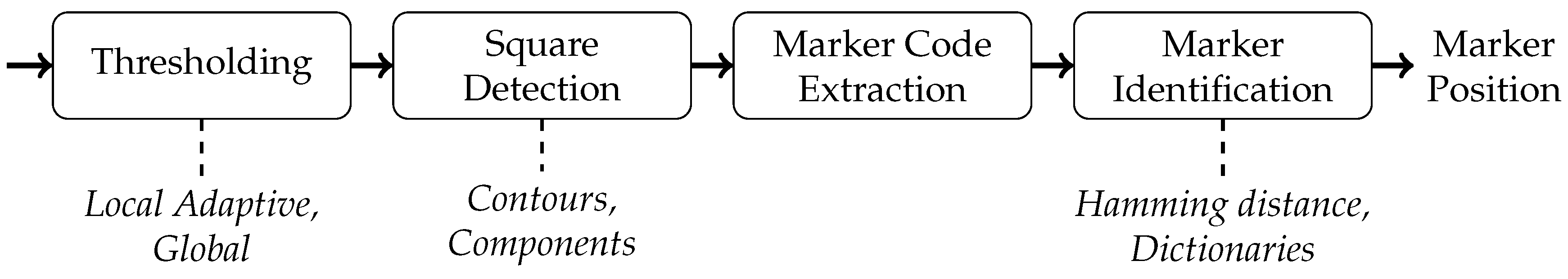
Marker detecting algorithms ARUco, ARUco3, and AprilTag2 follow the general structure described in Figure 1. First, the incoming image is thresholded using global or local adaptive methods to obtain a simplified binary image. This image is in the second step searched for square polygons that become candidates for markers. In the third step, identification code is extracted from inner area of each candidate, and the candidate is then in the fourth step identified and discarded if it does not belong to a set of valid codes. Finally, the position of the marker is computed from its corners or edges.

The ARUco detector [9] was designed to run fast and to recognize marker codes reliably. It uses an adaptive algorithm to threshold the input image, which computes the threshold value for each pixel as an average of the surrounding pixels. To detect marker-like shapes, it finds all contours and filters out those that do not represent square polygons (small contours, non-polygonal contours, etc.). After the squares are detected, it unprojects them to remove perspective distortion, thresholds them again (this time using the Otsu threshold), and obtains the inner code, which is checked with a dictionary to remove errors. If correct, the corners of these squares are used to compute their relative position to the camera.

The ARUco3 detector [10] is based on the ARUco detector and was improved to run fast with high-resolution images. There are two main differences between this algorithm and ARUco. The first difference is that this algorithm exchanges adaptive thresholding with simpler global thresholding, which is faster, but less robust to uneven lighting. The second difference is that it scales the image down, so that its size is still sufficient to detect and recognize markers, but the detection runs faster than in the original image. The implementation provided by the authors involves in three versions: Normal, Fast, and VideoFast. The Normal version uses adaptive thresholding like ARUco and therefore should be more robust to uneven illumination. The Fast version uses global thresholding and applies the Otsu method on an image part with a marker to compute the threshold for the next frame (or if no marker is available, it chooses the threshold randomly). The VideoFast version is like the Fast version, but additionally, it assumes that markers in a frame have approximately the same size as the markers in the previous frame and optimizes the scaling accordingly.

The AprilTag2 detector [12] also uses an adaptive algorithm for thresholding, but instead of using an average of all surrounding pixels, it searches these pixels for the lowest and highest intensities and chooses the threshold as the average between these two intensities. Then, it segments the binary result, fit quads, recovers codes, and uses a hash table to check if the code is correct and the quad is a marker.

2.2. Real-Time Algorithms Improving Underwater Images

In our previous work [35], we discussed the possibility of using real-time image-improving algorithms to increase the number of detected markers. The paper compared four algorithms, CLAHE, deblurring, white balancing (WB), and marker-based underwater white balancing (MBUWWB), which are also compared in this paper.

Contrast-limited adaptive histogram equalization (CLAHE) [50] is based on equalizing image histograms. At each pixel, it computes a histogram of its surroundings, rearranges it to avoid unnatural changes in contrast, and equalizes it to obtain new intensity. Deblur [51] (also known as deblurring or the unsharp mask filter) stresses edges by removing low frequencies from the original image, which can be described by the following equation:

$${\mathit{Image}}^{\mathit{out}}=(1+w)·{\mathit{Image}}^{\mathit{in}}-w·\mathit{Gaussian}({\mathit{Image}}^{\mathit{in}},{\sigma }_{\mathit{deblur}})$$

(1)

White balancing algorithms change the colors in the image to look more natural. There are many white-balancing algorithms, but for performance reasons, the authors in [35] chose a simple algorithm from [52]. This algorithm computes a histogram of input image, removes ${\mathit{perc}}_{\mathit{dark}}$ percent of the darkest pixels and $100-{\mathit{perc}}_{\mathit{bright}}$ percent of the brightest pixels, and changes the colors to stretch the rest of it linearly. Its adaptation for marker-based tracking, marker-based underwater white balancing, described also in [35], does the same, but computes the initial histogram only of areas that contain markers.

Many of these algorithms have parameters that influence their behavior. In the experiments presented in this paper, we use the same parameters as in [35]: 2 as a clip limit of CLAHE, 4 as both ${\sigma }_{\mathit{deblur}}$ and w for deblurring, and 2 as ${\mathit{perc}}_{\mathit{dark}}$ and 99 as ${\mathit{perc}}_{\mathit{bright}}$ for white balancing and marker-based underwater white balancing.

2.3. Detection of Markers under Water

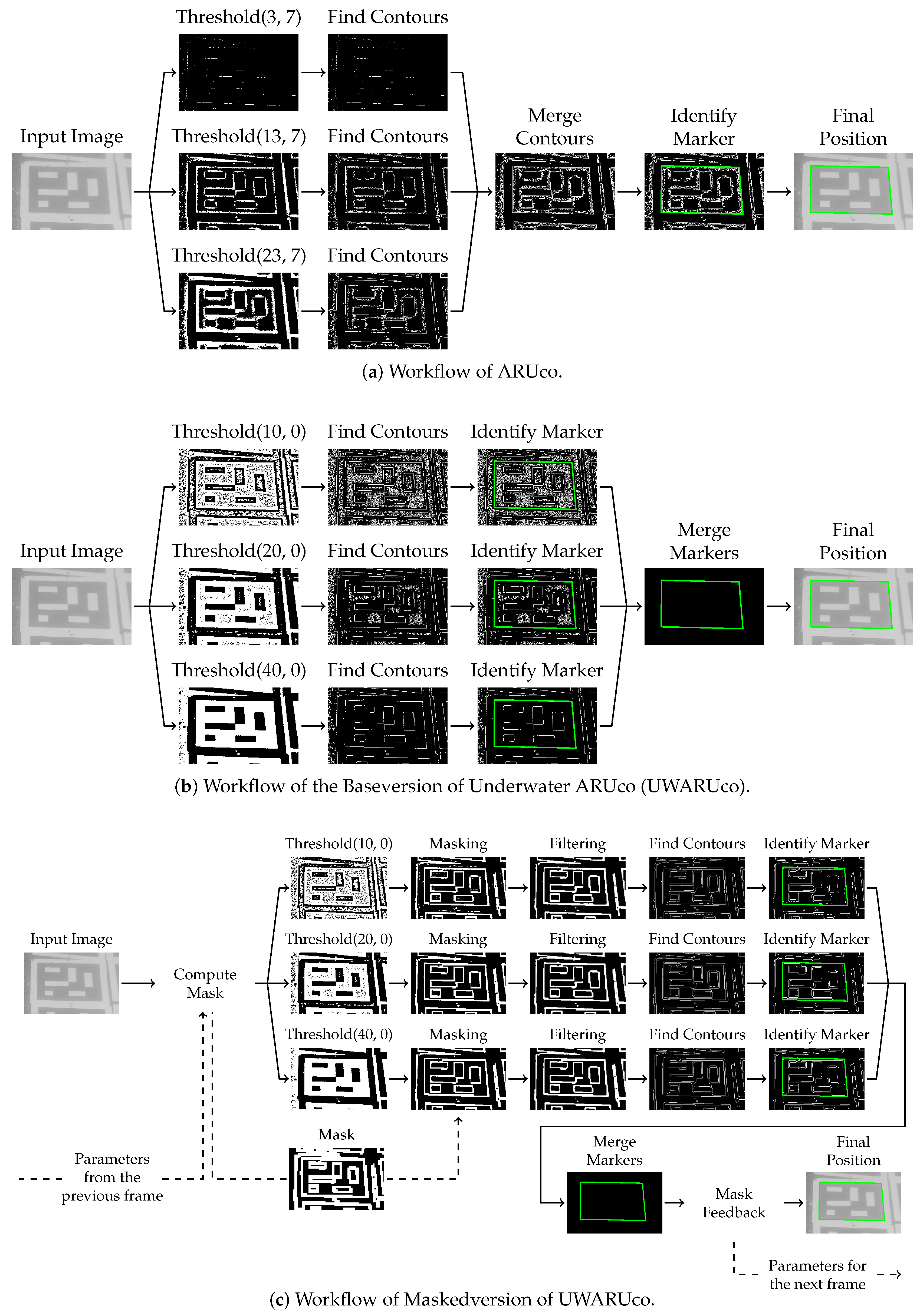
Underwater ARUco (UWARUco) is an adaptation of the ARUco algorithm [9] for underwater environments. The workflow of the original ARUco algorithm is shown in Figure 2a. It starts with an input grey-scale image, which is thresholded in the Threshold step and searches for contours in the Find Contours step three times in parallel threads, each time with different parameters of adaptive thresholding. The original algorithm used various sizes of the window that computed the threshold (by default, the sizes are 3, 13, and 23 pixels), and additionally, it decreased this threshold with a constant to suppress contours created by small noise (by default, this constant is seven). The contours found in each thresholded image are merged in the Merge Contours step to represent each marker with only one contour no matter how many thresholded images the contour is found in, and finally, in the Identify Marker step, the original image is thresholded again using the Otsu method to obtain the marker code that is identified. The algorithm is described in more detail in [9].

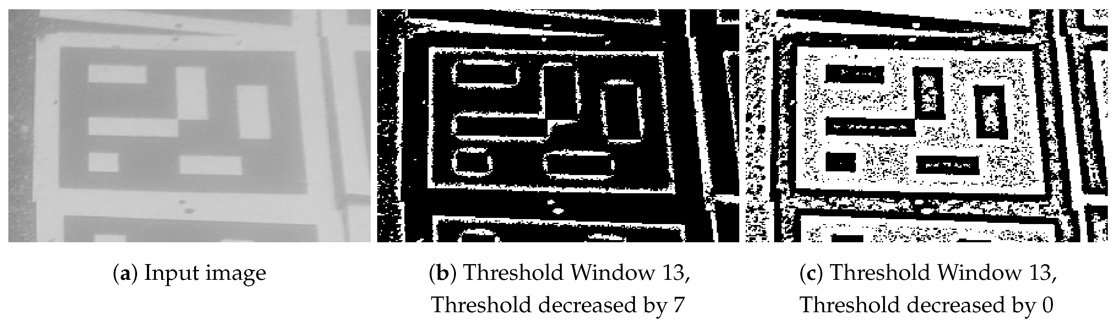
We analyzed the results presented in [35] to investigate which steps are influenced by image improving algorithms when the number of detected markers increases. In Figure 3a, we see an image of a marker taken in bad visibility conditions under water. When it is thresholded by ARUco, the marker’s border may get disconnected (see Figure 3b), and the marker is not recognized as a rectangular object. It was found that all four tested image-improving algorithms increased the contrast of the image, and additionally, deblur also acted as another blur applied to the image before thresholding. The same effect can be achieved by changing the parameters of the Threshold step to lower the constant decreasing the threshold and to increase the threshold window size, as is shown in Figure 3c, where the border stays connected when the threshold is not decreased. This change of parameters is not enough, since image-improving methods also affect the image that is thresholded by the Otsu method in the Identify Marker step. To solve this issue, the Identify Marker step is moved between the Find Contours step and the Merge Contours step (here renamed Merge Markers), and the identification is based on the thresholded image from the Threshold step instead of performing an additional threshold. These changes in the ARUco workflow form the base of our UWARUco algorithm. We call this algorithm the Base version of UWARUco and show its workflow in Figure 2b. Preliminary experiments showed that optimal window sizes for thresholding were 10, 20, and 40 pixels, and the constant that decreased the threshold was lowered to zero, i.e., the best results were obtained when the threshold was not decreased.

The Base version of UWARUco detects more markers in underwater videos than the original ARUco, as will be shown in Section 4 and Section 5.1. However, its processing time is slow, due to an increase in the number of contours that are found in thresholded images and that must be processed by the detector. To improve the processing speed of the detection, the algorithm is extended with a binary mask and a filter that are applied on the thresholded image before the contours are detected, to simplify the image and reduce the number of contours. We call this algorithm the Masked version of UWARUco; its workflow is shown in Figure 2c. This algorithm computes the binary mask from original image in the Compute Mask step. This step requires parameters derived in the previous video frame and creates a mask that is applied on thresholded images in the Masking steps. Before detecting contours in the Find Contour step, masked images are filtered in the Filtering steps to remove very small objects that appear in the image due to noise. After the results are merged in the Merge Markers step, the parameters for the next frame are derived from the input image and the result of detection in the Mask Feedback step.

The mask computed in the Compute Mask step identifies parts of image that do not contain markers and is composed of two submasks: brightness masks (Figure 4a) and noise masks (Figure 4b). The brightness mask detects parts of the image with very high intensity, since the brightest pixels are often white areas of markers and the noise mask removes areas that do not contain strong edges to keep only those parts that represent edges of markers. The final mask is created from parts that are in both masks, i.e., they are both very bright and contain a strong edge; see Figure 4c. The computation of the mask is described in Algorithm 1. First, the algorithm computes the minimum and maximum of intensities for blocks of $4\times 4$ pixels, which results in images $\mathit{mins}$ and $\mathit{maxs}$, which are in each dimension four-times smaller than the original image. These images are blurred to spread the minima and maxima of each pixel into its neighborhood by taking the minimum and maximum of a region of $3\times 3$ surrounding pixels. This blur is very important to keep the contours of markers connected, since without this blur, the mask will not contain areas where $4\times 4$ blocks are separated by marker contours, because in such cases, the blocks contain no strong edge and only one block is very bright. After blurring, the $\mathit{mins}$ image is subtracted from the $\mathit{maxs}$ image, and the difference is stored in the $\mathit{diffs}$ image. Finally, the $\mathit{maxs}$ image is thresholded by comparing it with a value of $\mathit{brightness}\_\mathit{threshold}$ and used for the brightness mask, and similarly, the difference image $\mathit{diffs}$ is compared to a value of $\mathit{noise}\_\mathit{threshold}$ to obtain the noise mask. At the end, both masks are ANDed together to obtain the final mask, which is applied in the Masking step. The effect of masking is illustrated in Figure 4d.

Algorithm 1: Pseudocode of the algorithm for computing the brightness mask, the noise mask, and the final mask.

Input: Grey scale image ${\mathit{Image}}^{\mathit{in}}$ whose mask is to be computed, threshold for brightness mask $\mathit{brightness}\_\mathit{threshold}$, threshold for noise mask $\mathit{noise}\_\mathit{threshold}$

Output: Brightness and noise masks $\mathit{brightness}\_\mathit{mask}$ and $\mathit{noise}\_\mathit{mask}$

$\mathit{mins}$ ← image of one fourth of the size of ${\mathit{Image}}^{\mathit{in}}$ with minimums of $4\times 4$ pixels of ${\mathit{Image}}^{\mathit{in}}$;

$\mathit{maxs}$ ← image of one fourth of the size of ${\mathit{Image}}^{\mathit{in}}$ with maximums of $4\times 4$ pixels of ${\mathit{Image}}^{\mathit{in}}$;

$\mathit{mins}\leftarrow$ minimum of $3\times 3$ surrounding pixels of $\mathit{mins}$;

$\mathit{maxs}\leftarrow$ maximum of $3\times 3$ surrounding pixels of $\mathit{maxs}$;

$\mathit{diffs}\leftarrow \mathit{maxs}-\mathit{mins}$;

$\mathit{brightness}\_\mathit{mask}\leftarrow \mathit{maxs}\ge \mathit{brightness}\_\mathit{threshold}$;

$\mathit{noise}\_\mathit{mask}\leftarrow \mathit{diffs}\ge \mathit{noise}\_\mathit{threshold}$;

$\mathit{final}\_\mathit{mask}\leftarrow \mathit{brightness}\_\mathit{mask}\wedge \mathit{noise}\_\mathit{mask}$;

The computation of thresholds $\mathit{brightness}\_\mathit{threshold}$ and $\mathit{noise}\_\mathit{threshold}$ is based on areas with detected markers and is done after the detection in the Mask Feedback step. The procedure is described in Algorithm 2. Images $\mathit{maxs}$ and $\mathit{diffs}$ that are used to compute masks are inspected at pixels of contours of found markers, and the lowest values of these pixels are used as thresholds. Such values would be sufficient as thresholds for the current frame, but to handle small changes in lighting between frames, they are decreased by $20\%$ to obtain actual thresholds for the following frame (this value was chosen after several experiments with different constants). If there are no contours, the thresholds are set to zero to disable masking in the following frame. Similarly, the thresholds are also set to zero before processing the very first frame of the video.

Algorithm 2: Pseudocode of the algorithm for computing thresholds for the brightness mask and the noise mask.

After applying the mask on the thresholded image, the result is filtered in the Filtering step using a $3\times 3$ median filter to remove small objects that appear due to the presence of noise. This filter removes pixel-sized objects and closes small holes, as illustrated in Figure 4e. Since the input image is binary, the median can be obtained fast by computing a mean of the surrounding pixels and thresholding it to a threshold of $0.5$.

3. Generating Synthetic Images

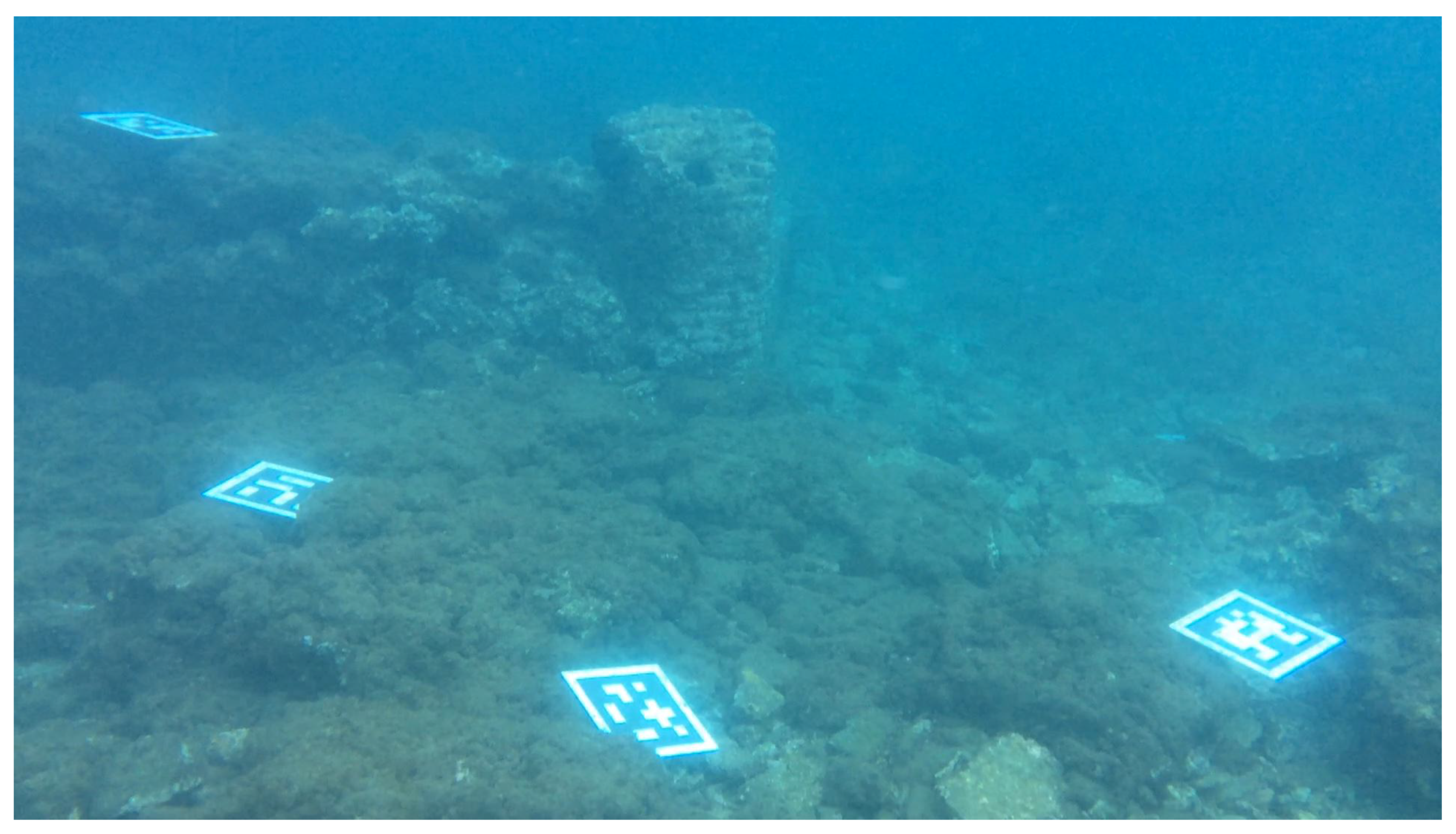
Our generator of synthetic images considers the following effects that appear under water: turbidity of water, glowing of markers, sensor noise, and a blur caused by not having objects perfectly focused. The effect of turbidity and glow in the real world is depicted in Figure 5.

The effect of turbidity simulates a decrease in visibility of distant objects, which is caused by very small particles dispersed in water. This effect is very close to the effect of fog, and for this reason, in the rest of the paper, we refer to this effect as the effect of fog. Small particles in water and post-processing effects in cameras also make markers glow, which happens when white areas of markers reflect a high amount of light (for example, when the marker is facing up), and this light is blurred due to the fog. This glow often makes white areas of the marker overexposed and black marker areas to have higher intensity than marker background. Sensor noise consists of thermal noise and other types of noise that appear when shooting images. We consider only thermal noise and simulate it with Gaussian random noise, as other types of noises can be either simulated as a part of this Gaussian noise or are not very significant. The effect of blur caused by objects that are not perfectly focused is added to avoid unnaturally sharp color changes of markers in images and is represented by Gaussian blur with a small sigma.

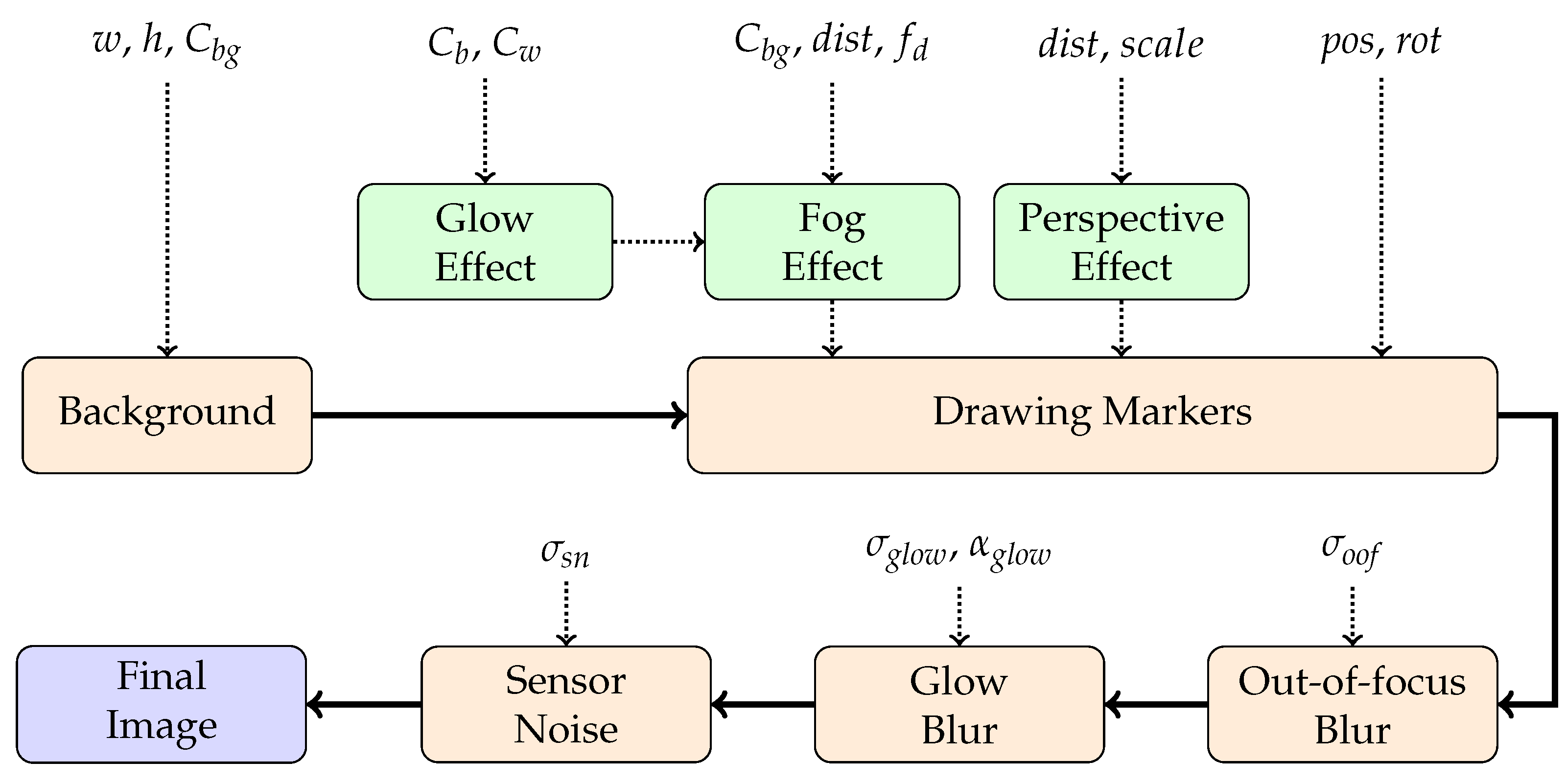
A pipeline of this image-generating algorithm is presented in Figure 6. It consists of five main steps that change the generated image (Background, Drawing Markers, Out-of-focus Blur, Glow Blur, and Sensor Noise), and three supporting steps that compute the parameters for main steps (Glow Effect, Fog Effect, and Perspective Effect).

The first step is the Background step. In this step, the image is allocated with width w and height h (in our experiments, we used images in full HD resolution: $1920\times 1080$ pixels) and filled with background color $C_{\mathit{bg}}$. In the Drawing Markers step, six markers are generated and rendered onto the background image with intensities $C_b$ and $C_w$ representing black and white marker regions. Each marker contains a $6\times 6$ pixels of binary code, one pixel of a black border, and one additional pixel of a white border, as if the marker were printed on a white square paper. Then, they are rotated with an angle $\mathit{rot}$, scaled by a factor $\mathit{scale}$, placed at position $\mathit{pos}$ to form a grid of two rows and three columns, and further displaced by up to 40 pixels.

Parameters $\mathit{scale}$, $C_b$, and $C_w$ are changed by supporting steps Glow Effect, Fog Effect, and Perspective Effect. In the Perspective Effect step, basic $\mathit{scale}$ is divided by the distance of the marker from the camera $\mathit{dist}$, so the markers that are further away are smaller. Intensities $C_b$ and $C_w$ are first increased in the Glow effect step and then mixed with background intensity $C_{bg}$ in the Fog effect step. The increase in intensity done by the glow effect depends on the experiment, but generally, this increase can be arbitrary. The mix done by the fog effect is based on Koschmieder’s model [53], which depends on the distance from the camera $\mathit{dist}$ and uses the following equation:

$$C_{\{\mathit{b},\mathit{w}\}}^{\mathit{out}}=C_{\{\mathit{b},\mathit{w}\}}^{\mathit{in}}·e^{-f_d·\mathit{dist}}+C_{\mathit{bg}}·(1-e^{-f_d·\mathit{dist}})$$

(2)

The third step called Out-of-focus Blur blurs the image very little to remove sharp changes in colors, which is done with a simple Gaussian blur with sigma ${\sigma }_{\mathit{oof}}$ (in all our images, this sigma was set to $1.0$). The glow effect not only changes the intensities of black and white areas of the marker, but also blurs the image. This blurred image is obtained by applying a Gaussian blur with sigma ${\sigma }_{\mathit{glow}}$, which is then mixed with the original image with factor ${\alpha }_{\mathit{glow}}$ to preserve sharp edges, as described in the following equation:

$${\mathit{Image}}^{\mathit{out}}=(1-{\alpha }_{\mathit{glow}})·{\mathit{Image}}^{\mathit{in}}+{\alpha }_{\mathit{glow}}·\mathit{Gaussian}({\mathit{Image}}^{\mathit{in}},{\sigma }_{\mathit{glow}})$$

(3)

In the last step, the Sensor Noise step, the image is changed by adding a sensor noise represented by Gaussian noise with zero mean and sigma ${\sigma }_{\mathit{sn}}$ (note that the intensities of pixels can be decreased, as well as increased in this step). The intensities of pixels are then clamped to range from 0–255 and written to the final image.

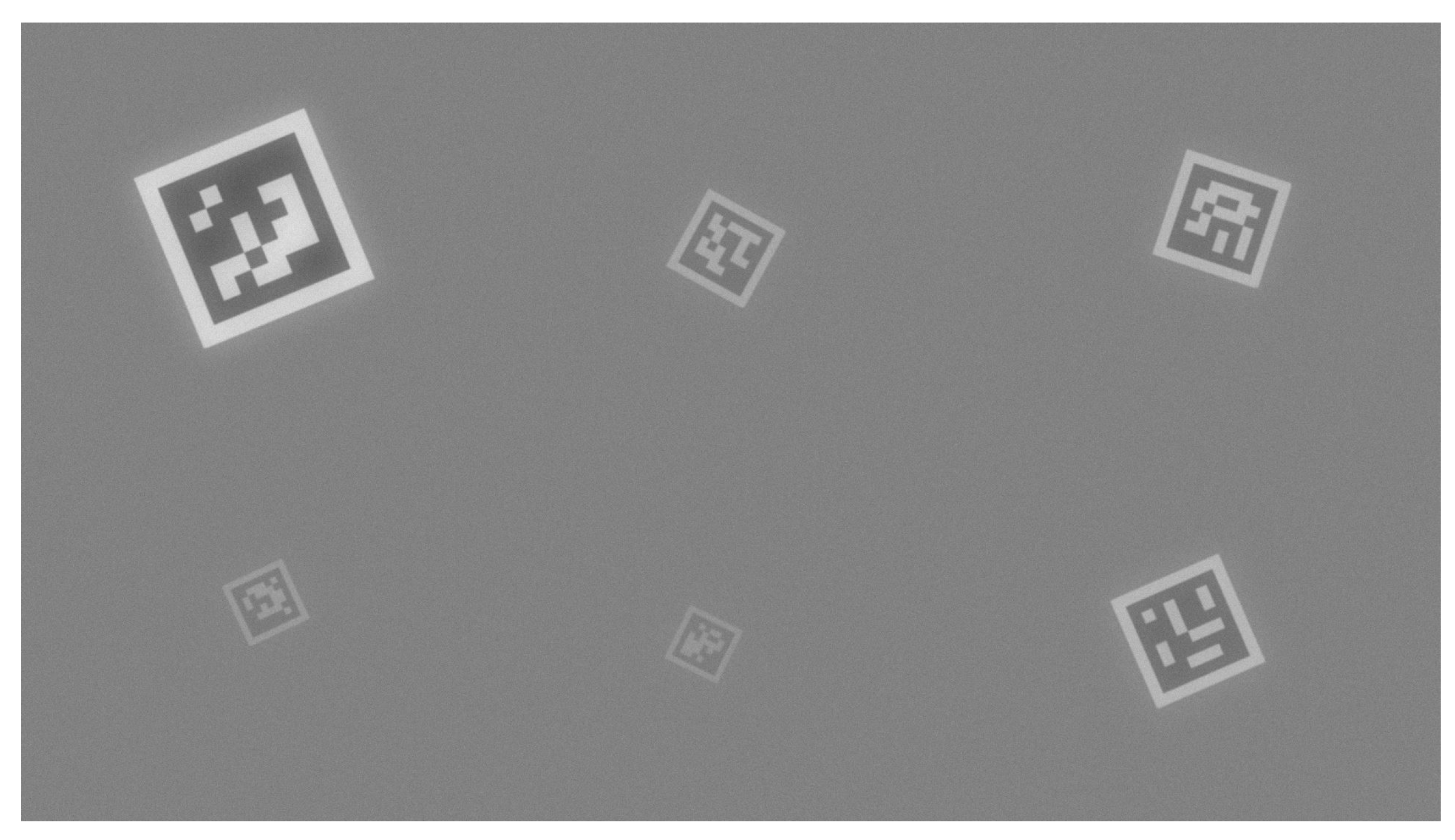
The generator does not generate images with markers that are occluded or severely deformed due to perspective transformations. An example of an image generated by this algorithm is presented in Figure 7.

4. Experiments with Synthetically-Generated Images

Synthetically-generated images were used in five experiments: a reference experiment with good conditions, an experiment simulating bad visibility conditions, an experiment simulating markers at different depths in foggy conditions, an experiment simulating glowing markers, and an experiment with all effects applied together. Experiments were performed on a desktop PC with a processor Intel Core i5 760, 8 GB of operating memory, and the operating system Windows 10, and the image-generating algorithm was implemented using the functions of OpenCV 3.4.3.

Processing time was computed only from frames that contained identified markers and followed after another frame with identified markers. This procedure provided better results regarding the performance of algorithms that utilize data from previous frames, because these algorithms are often optimized for such situations. If there were no such frames, the result was missing, as is visible in the graphs.

4.1. Reference with Good Visual Conditions

The first experiment evaluated the basic performance of marker detectors in very good visual conditions to obtain a reference for other results. In this test, fog effect, glow effect, perspective effect, and sensor noise effect were not applied, the intensity of the background was set to 150, the intensities of black and white marker colors were set to 0 and 255, respectively, and the scale of the markers was a variable parameter in this experiment, changing from 5–30 pixels. The intensity of the background was chosen to be a bit lighter that half-tone intensity to resemble real images, but did not influence the results, as observed in preliminary tests.

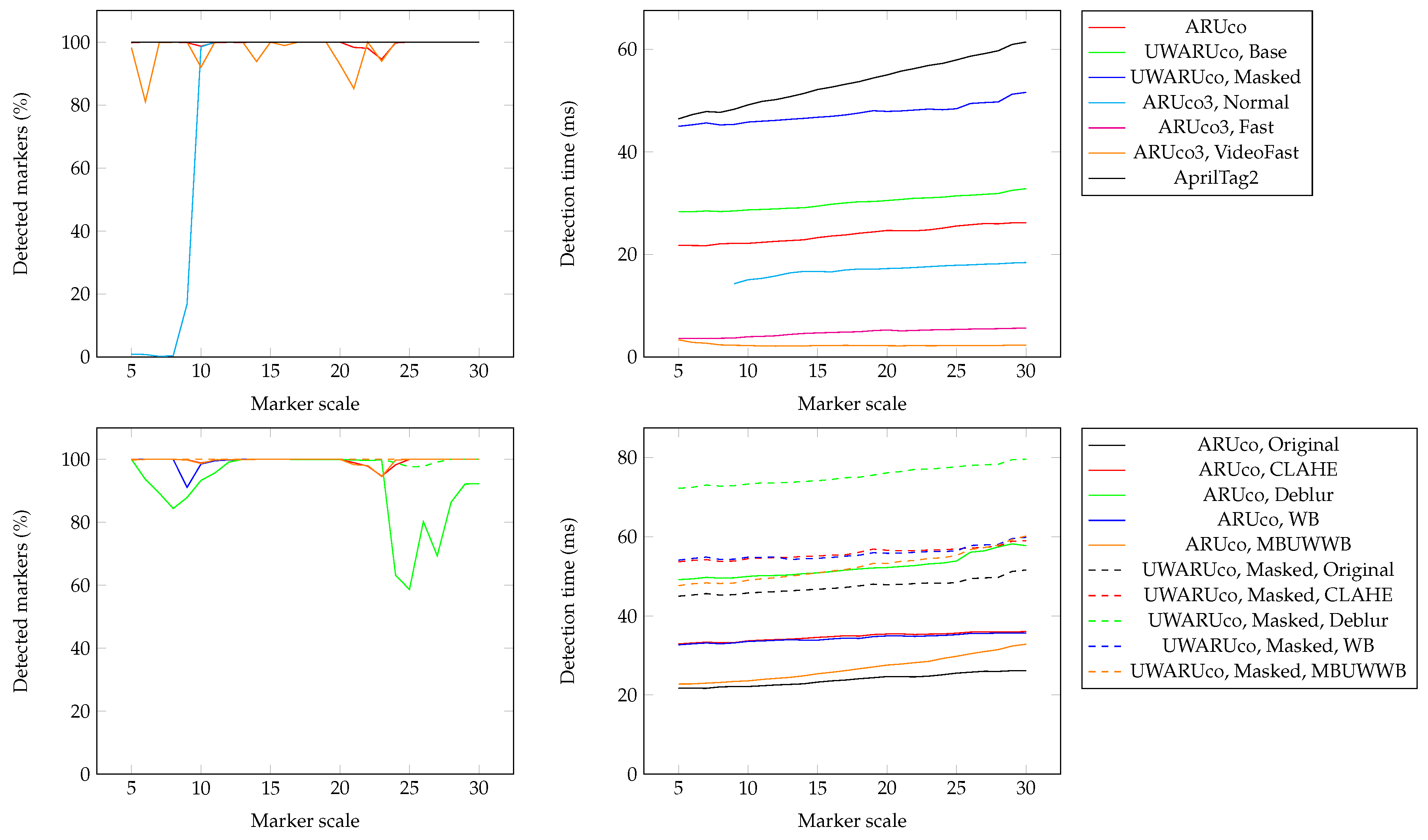
Each value of scale was tested in 20 videos consisting of 100 frames, and the results (percentage of detected markers and detection time) were averaged and are presented in Figure 8. It is shown that good visibility conditions were not a problem for any of the solutions, although some solutions had problems with specific scales of markers. The ARUco detector started to lose some markers when the scale of the marker was higher than 23 (the same value as the maximum window size of its adaptive thresholding algorithm). When the scale was larger, the thresholded image contained a fictional contour inside the marker border, and in some cases, this contour was chosen as the contour of the marker, which made the detected marker smaller and often not identified. This behavior was emphasized by some image-improving algorithms.

The Normal version of ARUco3 struggled to find small markers. Further tests found that this was caused by the white border around markers, which was too small, but when its size was increased, the number of detected markers reached 100%. The processing times show that the Fast and VideoFast variants of ARUco3 were clearly the fastest algorithms for the detection of markers in these very good visual conditions. Normal version of ARUco3 and ARUco provided the results at reasonable speeds, while the speed of UWARUco and ARUco combined with image-improving algorithms was lower, since these algorithms contained additional processing steps. The speed of AprilTag2 was also reasonably low in this test.

None of the solutions had problems with precision of detection, although this precision decreased with larger markers in the case of ARUco and UWARUco and their variants, because these detectors chose the wrong contours in some cases. However, even in these cases, the corners of markers were found with a precision of units of pixels.

4.2. Bad Visibility Conditions

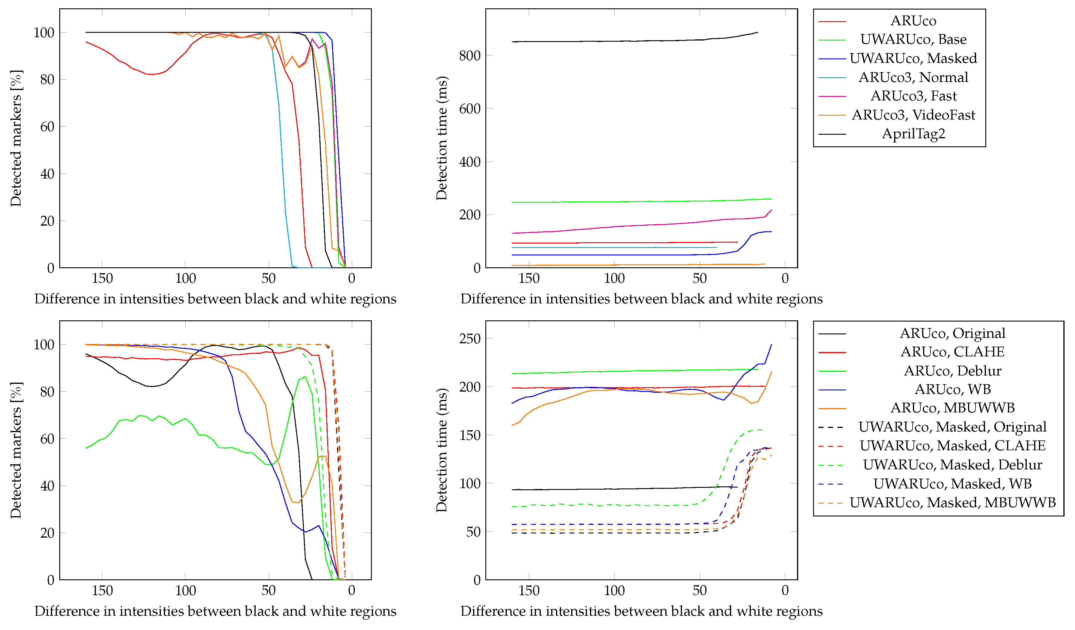
The task here was to simulate bad visibility conditions that cause lower contrast of the image. Glow and perspective effects were not applied; the intensity of the background was again set to 150; and the scale of all markers was set to 15 to prevent ARUco and UWARUco from choosing the wrong contours, as observed in the previous experiment. The sigma of sensor noise ${\sigma }_{\mathit{sn}}$ was set to five, which creates images that are similar to real images. The effect of fog was applied, but it was modified for this test. Since this effect changes only the difference between intensities of black and white regions of the marker, this difference became the main parameter of this analysis. Instead of depending on the distance $\mathit{dist}$ or fog density $f_d$, the intensities of black and white were set to specific values, starting at 70 and 230 to simulate a low-fog environment, and moving towards the intensity of the background, ending at 148 and 152 to simulate a high-fog environment. The difference between these intensities therefore started with 160 and ended with four.

The results are presented in Figure 9. In worse visibility conditions, the Fast and VideoFast versions of ARUco3 required more trials to find proper global threshold values, but when they did, they did not lose them, unless the visibility conditions were very bad. The decrease in the number of detected markers that was visible in the graphs was caused by a loss of markers in the first video frames. This experiment also showed that UWARUco was able to find markers in very bad conditions, being the last algorithm that detected markers when the difference between black and white regions became very low. AprilTag2 was also able to find markers in bad conditions, and so could the Fast and VideoFast versions of ARUco3 if they chose a good global threshold, but their results were worse than the results of UWARUco.

Image-improving algorithms did not perform well in this test. The results show that there was no need to improve images for UWARUco, and in the case of ARUco, the improvement in the number of detected markers was disputable, since the number of detected markers often increased in bad visibility conditions, but decreased in good visibility conditions.

The processing time was higher when compared to the times obtained in the reference, mainly due to the presence of sensor noise in the image. The processing time of AprilTag2 increased greatly, which makes this algorithm unusable in real-time solutions. The processing times of ARUco, the Base version of UWARUco, and the Normal and Fast versions of ARUco3 also increased, but less than then the time of AprilTag2. The processing time of the Masked version of UWARUco remained the same as in the reference, so it became faster than the other algorithms, whose processing time increased. The fastest solution of this test was the VideoFast version of ARUco3, but it detected fewer markers.

4.3. Foggy Conditions and Markers at Different Distances

Here, markers were placed in a foggy environment at different distances from the viewer, which influenced their size and also their contrast, due to the presence of fog. This distance was set between values of $1.0$ and $4.0$ and changed continuously between successive frames, since abrupt changes could negatively influence marker detectors that use data from previous frames. The scale of the markers started at 30 at a distance of $1.0$ and decreased linearly with the distance; the intensity of the background was again fixed at 150; the intensities of black and white marker regions were zero and 255 at zero distance; the glow effect was not present; and the sigma of sensor noise ${\sigma }_{\mathit{sn}}$ was again set to five. The density of the fog was set to $f_d=1.0$, so that the difference in intensities between black and white regions at maximum depth was approximately five, as in the previous test when choosing the worst conditions.

This test had no variable parameter, so only one set of 20 videos with 100 frames was generated. The results are presented in

Table 1. Results of the test with markers at different distances.

Solution	ARUco	UWARUco Base	UWARUco Masked	ARUco3 Normal	ARUco3 Fast	ARUco3 VideoFast	AprilTag2
Detected markers (%)	32.067	64.658	75.050	24.000	60.392	45.450	51.342
Detection time (ms)	96.002	255.633	117.907	76.769	89.064	9.564	1220.796
Solution	ARUco Original	ARUco CLAHE	ARUco Deblur	ARUco WB	ARUco MBUWWB
Detected markers (%)	32.067	63.225	43.808	46.025	57.525
Detection time (ms)	96.002	201.421	218.623	200.801	193.417
Solution	UWARUco Masked Original	UWARUco Masked CLAHE	UWARUco Masked Deblur	UWARUco Masked WB	UWARUco Masked MBUWWB
Detected markers (%)	75.050	79.525	58.500	77.992	77.358
Detection time (ms)	117.907	128.644	141.740	128.436	117.376

. The Masked version of UWARUco detected the highest number of markers, while its processing time was comparable with other algorithms, with the exception of the VideoFast version of ARUco3, which was faster, but detected a lower number of markers. The results of image improving algorithms show that in this test, they were able to increase the number of detected markers of ARUco at the cost of higher detection time, some of them placing ARUco at approximately the same level as the Base version of UWARUco. They also slightly improved the results of the Masked version of UWARUco, again at the cost of increased processing time.

4.4. Glowing Markers

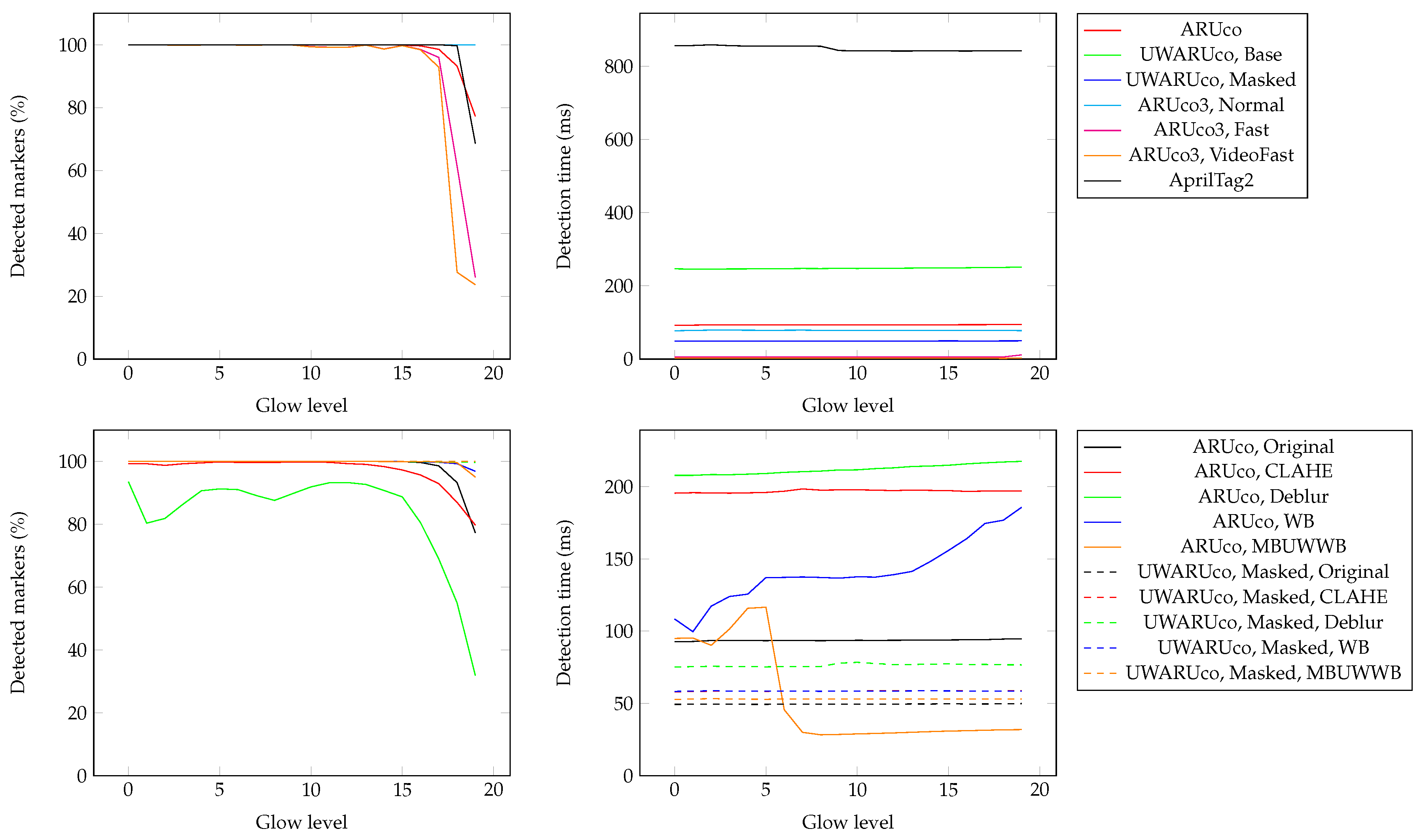
Next, the detection of markers in foggy environments that appeared to glow in the image was evaluated. Perspective and fog effects were not applied; the scale of markers was set to 15; and the sigma of sensor noise was set to ${\sigma }_{\mathit{sn}}=5$. The intensity of the background was set to a low value of 50, so that black marker areas could have higher intensity than the background. The glow effect was simulated with 20 levels, each level increasing the intensity of the black marker areas linearly from 0–100, the intensity of white marker areas from 255–400, the glow alpha ${\alpha }_{\mathit{glow}}$ from $0.0$–$0.8$, and the glow sigma ${\sigma }_{\mathit{glow}}$ from 0–60.

As with the previous experiments, each glow effect level was tested with 20 videos consisting of 100 frames. The averaged results are presented in Figure 10. Several marker-detecting algorithms (ARUco, the Fast and VideoFast versions of ARUco3, and AprilTag2) struggled to find markers when the glow was at high levels: the Fast and VideoFast variants of ARUco3 again lost several frames until they found the proper global threshold value. The processing time of all detectors stayed approximately the same without any influence caused by an increased level of glow. Since the number of detected markers was already very high, image-improving algorithms could not increase these values. Some of them (CLAHE and deblur combined with ARUco) decreased the number of detected markers, but many of them just increased the computation time. One exception to this was the combination of ARUco and MBUWWB, which decreased the computation time at glow levels above six, while keeping the number of detected markers very high. This happened because at glow levels higher than six, black marker regions had higher intensity than the background, so most of the artificial sensor noise was removed, which made the thresholded image mostly noise-free.

4.5. All Effects

Finally, all effects affecting synthetically-generated images were incorporated. Several variables were changed at the same time, continuously between successive frames. To focus more on the bad visibility conditions, the values were chosen to obtain a difference between the black and white areas that was lower than 100 and a glow level between 10 and 20: the intensity of background $C_{\mathit{bg}}$ was changed between values of 50 and 200, the distance of markers $\mathit{dist}$ between values of $1.5$ and $4.0$, and intensity of fog $f_d$ between values of $0.6$ and $1.0$. Additionally, the intensity of the glow effect was changed to influence the intensity of black and white regions of markers, glow alpha, and glow sigma simultaneously. The intensity of black regions $C_b$ was changed between values of 50 and 100, the intensity of white regions $C_w$ between values of 330 and 400, glow alpha ${\alpha }_{\mathit{glow}}$ between values of $0.4$ and $0.8$, and glow sigma ${\sigma }_{\mathit{glow}}$ between values of 30 and 60. As in the previous experiments, the scale of markers was kept the same at a value of 30 at a distance of one and the sigma of sensor noise ${\sigma }_{\mathit{sn}}$ at a value five.

This test also had no variable parameter, so only one set of 20 videos with 100 frames was generated. The results are presented in

Table 2. Results of the test with all effects active.

Solution	ARUco	UWARUco Base	UWARUco Masked	ARUco3 Normal	ARUco3 Fast	ARUco3 VideoFast	AprilTag2
Detected markers (%)	7.967	63.533	72.683	1.875	25.892	18.075	28.900
Detection time (ms)	97.862	263.899	128.422	77.829	56.790	6.979	871.732
Solution	ARUco Original	ARUco CLAHE	ARUco Deblur	ARUco WB	ARUco MBUWWB
Detected markers (%)	7.967	42.417	19.767	19.783	21.342
Detection time (ms)	97.862	200.967	219.783	206.210	195.214
Solution	UWARUco Masked Original	UWARUco Masked CLAHE	UWARUco Masked Deblur	UWARUco Masked WB	UWARUco Masked MBUWWB
Detected markers (%)	72.683	74.992	47.608	73.125	68.633
Detection time (ms)	128.422	136.058	156.065	117.667	94.246

. The highest number of detected markers was obtained by both versions of UWARUco, with the Masked version detecting nearly 73% of markers at times lower than the other algorithms (except for ARUco3). This shows that UWARUco, especially its Masked version, is best suited for underwater environments. The Fast and VideoFast versions of ARUco3 algorithm detected less than 26% of markers, though their detection time was very low, especially in the case of the VideoFast version. AprilTag2 detected nearly 29% of markers, but at a very high computation time. The original ARUco did not detect even 8% of markers.

The results of image-improving techniques were rather surprising, because in previous experiments, these methods gave promising results only when detecting markers at different distances, but in other tests, they decreased the number of detected markers. Here, these methods increased the number of detected markers, although again at an increased time of detection. This result is similar to that obtained in [35] when tested on real images.

Discussion of Synthetic Images

The synthetic generation of images is able to test many situations that appear in underwater environments; however, some of these situations were not tackled. One limitation of the generated images is that all markers were facing the camera, but this problem of skewed markers or markers under severe perspective deformations is not bound solely to underwater environments and requires the construction of a specialized marker detectors to deal with it. In our experience with real images, the detection of markers was also influenced by objects that obscured markers, be it floating objects like fish or static objects like surrounding rocks and plants. As with the previous issue, the solution to this problem requires a specialized marker detector.

All tested images also had a single-color background, which does not appear in real images, since the background is made of various objects. The algorithm for generating images can be improved by swapping the background with an image or a video that is taken under water, but this solution requires many videos in different environments with well-assessed parameters for the effect, to fit the generated markers seamlessly into images, and to prevent the results from being shifted towards specific videos.

The results of the tests do not mention a number of falsely-detected markers. Unless we included the results with mischosen contours as described in Section 4.1, falsely-detected markers appeared extremely rarely. From 176,000 frames processed by 15 combinations of marker-detecting and image-improving algorithms, only 110 falsely-detected markers appeared, detected by ARUco (1), ARUco with CLAHE (10), ARUco with deblur (11), ARUco with WB (11), ARUco with MBUWWB (7), the Masked version of UWARUco (5), the Masked version of UWARUco with CLAHE (3), the Masked version of UWARUco with deblur (4), the Masked version of UWARUco with WB (2), the Masked version of UWARUco with MBUWWB (6), and AprilTag2 (50). The Base version of UWARUco and all versions of ARUco3 did not report any false positive.

5. Evaluation of Real Underwater Images

Marker-detecting solutions were also compared on images taken under water in the Mediterranean Sea. This experiment reported only the number of detected markers and the processing time, and not the precision of the detection, for the following reasons. First, the divers were unable to measure the location of markers with a sufficient precision, which requires being very high, since the experiments with synthetic images found that the ground truth location of markers must be known with a precision of units of pixels. Second, due to the high number of frames, bad visibility conditions, and required precision, the ground truth was infeasible to obtain manually.

The parameters of videos are shown in

Table 3. Evaluated sets of videos. Abbreviations: Nm: name of the set; Lc: location where the set was taken; Tr: assessed level of turbidity; Dp: depth at which the set was taken; Dv: recording device; Rs: resolution of the video; Cm: compression method; FL: frame rate and length in seconds. Location B., It. stands for Baiae, Italy.

Nm:	Baiae1	Nm:	Athens	Nm:	Constandis
Lc:	Baiae, Italy	Lc:	Athens, Greece	Lc:	Limassol, Cyprus
Tr:	High	Tr:	Moderate	Tr:	Moderate
Dp:	5–6 m	Dp:	7–9 m	Dp:	20–22 m
Dv:	iPad Pro 9.7 inch	Dv:	GoPro camera	Dv:	GARMIN VIRB XE
Rs:	1920 × 1080	Rs:	1920 × 1080	Rs:	1920 × 1440
Cm:	MPEG-2	Cm:	MPEG-4	Cm:	MPEG-4
FL:	30 fps, 85 s	FL:	30 fps, 31 s	FL:	24 fps, 160 s
Nm:	Green Bay	Nm:	Villa	Nm:	Baiae2
Lc:	Green Bay, Cyprus	Lc:	Villa a Protiro, B., It.	Lc:	Baiae, Italy
Tr:	Low	Tr:	Moderate	Tr:	Moderate
Dp:	7–9 m	Dp:	5–6 m	Dp:	5–6 m
Dv:	NVIDIA SHIELD	Dv:	Samsung Galaxy S8	Dv:	iPad Mini 2
Rs:	1920 × 1080	Rs:	1920 × 1080	Rs:	1920 × 1080
Cm:	MPEG-4	Cm:	no compression	Cm:	MPEG-4
FL:	30 fps, 81 s	FL:	30 fps, 141 s	FL:	30 fps, 421 s
		Nm:	Epidauros
		Lc:	Epidauros, Greece
		Tr:	Low
		Dp:	4–6 m
		Dv:	Sony FDR-X1000V
		Rs:	3840 × 2160
		Cm:	MPEG-4
		FL:	24 fps, 180 s

. This table describes the level of turbidity in the videos, the depth under the sea at which the videos were taken, the device that took the video, the resolution of the video, the compression algorithm, the frame rate, and the length in seconds. Sets Baiae1, Athens, Constandis, and Green Bay were taken from [1] and set Villa from [35], and sets Baiae2 and Epidauros are new. It should be noted that the level of visibility is only illustrative; it is not based on any measurement and was chosen by the authors by assessing the videos.

Sets Baiae1, Athens, Constandis, and Green Bay contained a board with six markers from the ARUco library, each with a size of 8 cm. Set Athens also contained a single separate marker with a size of 16 cm, and sets Villa and Epidauros contained nine separate markers of a size of 19 cm, placed into a grid of $3\times 3$ markers. In set Baiae2, separate markers of a of size 19 cm were placed isolated from each other on the ground around other objects. Measuring was performed on the same computer that ran the experiments with the synthetically-generated videos. Computation time was also evaluated only on frames with detected markers if they followed another frame with detected markers.

5.1. Results of Underwater Tests

The total number of detected markers and average processing time are shown in

Table 4. Results of detecting markers in real underwater videos.

Solution		ARUco	UWARUco Base	UWARUco Masked	ARUco3 Normal	ARUco3 Fast	ARUco3 VideoFast	AprilTag2
Baiae1	# of markers	467	6004	6223	36	2145	1893	5695
	Time (ms)	24.627	111.528	57.680	15.397	6.970	1.748	178.874
Athens	# of markers	5272	5913	5832	4877	5565	2610	5923
	Time (ms)	31.202	86.503	53.771	21.398	6.550	2.843	240.672
Constandis	# of markers	6981	6944	6878	6578	5382	4511	6332
	Time (ms)	39.010	139.514	65.565	25.030	6.672	5.446	327.887
Green Bay	# of markers	7964	7932	7594	7062	6347	5784	7332
	Time (ms)	27.531	74.712	49.915	18.040	10.537	5.288	222.003
Villa	# of markers	14,457	19,879	20,145	9947	14,316	12,589	20,082
	Time (ms)	75.747	140.659	62.872	58.266	6.700	2.368	323.005
Baiae2	# of markers	13,829	15,932	14,976	12,466	8257	3869	14,577
	Time (ms)	34.552	83.614	55.093	21.535	4.563	1.672	230.910
Epidauros	# of markers	18,749	25,126	25,713	13,864	10,480	6340	21,628
	Time (ms)	181.441	425.286	252.327	152.590	23.575	4.692	1252.122
Solution		ARUco Original	ARUco CLAHE	ARUco Deblur	ARUco WB	ARUco MBUWWB
Baiae1	# of markers	467	3646	3857	4098	5140
	Time (ms)	24.627	38.064	80.560	43.370	47.475
Athens	# of markers	5272	5504	5611	5640	5616
	Time (ms)	31.202	48.424	86.524	45.867	38.271
Constandis	# of markers	6981	6279	6850	6737	6869
	Time (ms)	39.010	73.406	136.165	86.436	53.236
Green Bay	# of markers	7964	6406	8355	7392	7896
	Time (ms)	27.531	49.000	84.394	50.442	35.355
Villa	# of markers	14,457	18,981	18,958	19,029	19,398
	Time (ms)	75.747	138.263	178.143	114.494	45.239
Baiae2	# of markers	13,829	14,126	11,445	11,500	10,227
	Time (ms)	34.552	62.603	100.112	50.598	27.755
Epidauros	# of markers	18,749	20,030	23,597	16,929	21,696
	Time (ms)	181.441	341.750	586.785	296.562	181.483
Solution		UWARUco Masked Original	UWARUco Masked CLAHE	UWARUco Masked Deblur	UWARUco Masked WB	UWARUco Masked MBUWWB
Baiae1	# of markers	6223	6612	6081	6129	5605
	Time (ms)	57.680	64.902	93.618	64.998	55.866
Athens	# of markers	5832	5806	5848	5831	5829
	Time (ms)	53.771	60.742	85.729	60.054	52.622
Constandis	# of markers	6878	6702	6959	6749	6843
	Time (ms)	65.565	75.938	105.121	76.404	68.263
Green Bay	# of markers	7594	6776	7464	7149	7599
	Time (ms)	49.915	56.289	78.405	56.515	51.390
Villa	# of markers	20,145	20,281	19,400	20,225	20,258
	Time (ms)	62.872	82.574	114.332	65.231	61.647
Baiae2	# of markers	14,976	15,996	15,356	12,988	13,244
	Time (ms)	55.093	65.498	85.929	62.256	55.415
Epidauros	# of markers	25,713	26,012	23,618	21,991	25,623
	Time (ms)	252.327	305.263	388.771	274.608	247.548

. ARUco was able to detect markers in videos with medium visibility (Villa, Baiae2), but struggled to detect markers in poor visibility conditions (Baiae1). The results were better when using image-improving techniques; however, no technique provided the best result in all sets. MBUWWB provided good results in Villa and especially in Baiae1, but it struggled with the detection of markers in set Baiae2, where the markers were at different distances from the viewer, which also means their visibility was different. This represents a complication for MBUWWB, because this technique is a global technique (as well as other techniques, e.g., WB), and it changes the whole image in the same manner. The ARUco3 detector also did not produce consistent results; the table shows that in the case of Villa, the Fast version of this detector detected the highest number of markers and the Normal version found the lowest number of markers, but an opposite result was found in Baiae2 and other sets. It must be noted, however, that both the Fast and VideoFast versions are also global techniques and exhibited similar problems as the MBUWWB image-improving technique. AprilTag2 was able to detect a very high number of markers in most situations; however, its processing time was also very high and therefore hard to use in real-time augmented reality applications, especially when targeting mobile devices.

The Base version of UWARUco consistently detected a very high number of markers. This was compensated by its processing time, which was also higher: it was higher than the processing times of original ARUco and all versions of ARUco3, approximately the same as the processing times of slower combinations of ARUco and image-improving algorithms, and still lower than the processing times of AprilTag2. However, the results of the Masked version of UWARUco show that the number of detected markers can still be very high while the processing time was much lower. They also show that using additional image-improving techniques is not necessary, although using some of them can still lead to better results at the price of increased processing time.

5.2. Discussion of Underwater Experiments

The comparison between the results of the Base and Masked versions of UWARUco shows that the number of detected markers can increase when the thresholded image is masked before detecting contours. This unexpected outcome happens because this mask does not remove contours; instead, it merges them into larger contours, which can connect borders of markers that are disconnected in the original image, therefore detecting a marker that is not detected in the original image.

According to [10], ARUco3 was designed to run fast with high-resolution images at the price of reducing its adaptability to worse visibility and lighting conditions. This is confirmed in the results: the Fast and VideoFast versions of ARUco3 provided the fastest processing times when compared to other methods, but the number of detected markers dropped in worse visibility conditions. The number of false positives was not counted in this experiment, since the ground truth solution was missing. However, it is expected to be very low, like in the previous test with synthetically-generated images.

6. Conclusions

This paper presented a method for generating synthetic images of square markers in bad visibility conditions in underwater environments that focuses on high turbidity and glowing markers, as well as a new algorithm for detecting markers in such environments called UWARUco. This algorithm is based on the ARUco marker detector, but replaces its method for reducing the number of contours caused by noise with a method that masks out areas that do not contain any markers. In simulated bad visibility conditions, our solution detected almost three-times more markers than state-of-the-art robust solutions, while increasing the processing time by 30% when compared to ARUco. In real underwater environments, it detected between 95% and 290% of markers detected by other solutions suitable for real-time AR, while keeping 83–234% of the ARUco processing time, depending on the environment.

Future work will be focused on the fusion of this algorithm with other methods that are used to compute and maintain the orientation of a mobile device. Using techniques like the Kalman filter, the position obtained visually by detecting markers will be fused with the results of internal device sensors like the accelerometer or gyroscope and devices that are able to provide absolute position underwater like acoustic beacons. This will create a sophisticated solution for underwater augmented reality, which can be deployed in applications that present underwater cultural heritage to the general public or to help divers with orientation in deep underwater archaeological sites.

References

- Skarlatos, D.; Agrafiotis, P.; Balogh, T.; Bruno, F.; Castro, F.; Petriaggi, B.D.; Demesticha, S.; Doulamis, A.; Drap, P.; Georgopoulos, A.; et al. Project iMARECULTURE: Advanced VR, iMmersive Serious Games and Augmented REality as Tools to Raise Awareness and Access to European Underwater CULTURal Heritage; Digital Heritage; Springer International Publishing: Cham, Switzerland, 2016; pp. 805–813. [Google Scholar]
- Edney, J.; Spennemann, D.H.R. Can Artificial Reef Wrecks Reduce Diver Impacts on Shipwrecks? The Management Dimension. J. Marit. Archaeol. 2015, 10, 141–157. [Google Scholar] [CrossRef]
- Vlahakis, V.; Ioannidis, N.; Karigiannis, J.; Tsotros, M.; Gounaris, M.; Stricker, D.; Gleue, T.; Daehne, P.; Almeida, L. Archeoguide: An Augmented Reality Guide for Archaeological Sites. IEEE Comput. Graph. Appl. 2002, 22, 52–60. [Google Scholar] [CrossRef]
- Panou, C.; Ragia, L.; Dimelli, D.; Mania, K. An Architecture for Mobile Outdoors Augmented Reality for Cultural Heritage. ISPRS Int. J. Geo-Inf. 2018, 7. [Google Scholar] [CrossRef]
- Von Lukas, U.F. Underwater Visual Computing: The Grand Challenge Just around the Corner. IEEE Comput. Graph. Appl. 2016, 36, 10–15. [Google Scholar] [CrossRef] [PubMed]
- Kato, H.; Billinghurst, M. Marker Tracking and HMD Calibration for a Video-Based Augmented Reality Conferencing System. In Proceedings of the 2nd IEEE and ACM International Workshop on Augmented Reality, San Francisco, CA, USA, 20–21 October 1999; pp. 85–94. [Google Scholar] [CrossRef]
- Wagner, D.; Schmalstieg, D. ARToolKitPlus for Pose Tracking on Mobile Devices. Proceedings of 12th Computer Vision Winter Workshop, St. Lambrecht, Austria, 6–8 February 2007; pp. 139–146. [Google Scholar]
- Fiala, M. ARTag, a Fiducial Marker System Using Digital Techniques. In Proceedings of the 2005 IEEE Computer Society Conference on Computer Vision and Pattern Recognition (CVPR’05), San Diego, CA, USA, 20–25 June 2005; IEEE Computer Society: Washington, DC, USA, 2005; pp. 590–596. [Google Scholar] [CrossRef]
- Garrido-Jurado, S.; noz Salinas, R.M.; Madrid-Cuevas, F.J.; Marín-Jiménez, M.J. Automatic Generation and Detection of Highly Reliable Fiducial Markers under Occlusion. Pattern Recognit. 2014, 47, 2280–2292. [Google Scholar] [CrossRef]
- Romero-Ramirez, F.J.; noz Salinas, R.M.; Medina-Carnicer, R. Speeded up detection of squared fiducial markers. Image Vis. Comput. 2018, 76, 38–47. [Google Scholar] [CrossRef]
- Olson, E. AprilTag: A robust and flexible visual fiducial system. In Proceedings of the 2011 IEEE International Conference on Robotics and Automation, Shanghai, China, 9–13 May 2011; pp. 3400–3407. [Google Scholar] [CrossRef]
- Wang, J.; Olson, E. AprilTag 2: Efficient and robust fiducial detection. In Proceedings of the IEEE/RSJ International Conference on Intelligent Robots and Systems (IROS), Beijing, China, 9–15 October 2016. [Google Scholar]
- Naimark, L.; Foxlin, E. Circular Data Matrix Fiducial System and Robust Image Processing for a Wearable Vision-Inertial Self-Tracker. In Proceedings of the International Symposium on Mixed and Augmented Reality, Darmstadt, Germany, 30 September–1 October 2002; pp. 27–36. [Google Scholar] [CrossRef]
- Köhler, J.; Pagani, A.; Stricker, D. Robust Detection and Identification of Partially Occluded Circular Markers. In Proceedings of the VISAPP 2010—Fifth International Conference on Computer Vision Theory and Applications, Angers, France, 17–21 May 2010; pp. 387–392. [Google Scholar]
- Bergamasco, F.; Albarelli, A.; Cosmo, L.; Rodolá, E.; Torsello, A. An Accurate and Robust Artificial Marker Based on Cyclic Codes. IEEE Trans. Pattern Anal. Mach. Intell. 2016, 38, 2359–2373. [Google Scholar] [CrossRef] [PubMed]
- Bencina, R.; Kaltenbrunner, M.; Jorda, S. Improved Topological Fiducial Tracking in the reacTIVision System. In Proceedings of the 2005 IEEE Computer Society Conference on Computer Vision and Pattern Recognition (CVPR’05)—Workshops, San Diego, CA, USA, 20–25 June 2005. [Google Scholar]
- Toyoura, M.; Aruga, H.; Turk, M.; Mao, X. Detecting Markers in Blurred and Defocused Images. In Proceedings of the 2013 International Conference on Cyberworlds, Yokohama, Japan, 21–23 October 2013; pp. 183–190. [Google Scholar] [CrossRef]
- Xu, A.; Dudek, G. Fourier Tag: A Smoothly Degradable Fiducial Marker System with Configurable Payload Capacity. In Proceedings of the 2011 Canadian Conference on Computer and Robot Vision, St Johns, NL, Canada, 25–27 May 2011; pp. 40–47. [Google Scholar] [CrossRef]
- Lowe, D.G. Object recognition from local scale-invariant features. In Proceedings of the Seventh IEEE International Conference on Computer Vision, Corfu, Greece, 20–25 September 1999; Volume 2, pp. 1150–1157. [Google Scholar] [CrossRef]
- Gordon, I.; Lowe, D.G. Scene modelling, recognition and tracking with invariant image features. In Proceedings of the Third IEEE and ACM International Symposium on Mixed and Augmented Reality, Arlington, VA, USA, 2–5 November 2004; pp. 110–119. [Google Scholar] [CrossRef]
- Bay, H.; Tuytelaars, T.; Van Gool, L. SURF: Speeded Up Robust Features. In Proceedings of the Computer Vision—ECCV 2006, Graz, Austria, 7–13 May 2006; Leonardis, A., Bischof, H., Pinz, A., Eds.; Springer: Berlin/Heidelberg, Germany, 2006; pp. 404–417. [Google Scholar]
- Rosten, E.; Drummond, T. Machine Learning for High-Speed Corner Detection. In Proceedings of the Computer Vision—ECCV 2006, Graz, Austria, 7–13 May 2006; Leonardis, A., Bischof, H., Pinz, A., Eds.; Springer: Berlin/Heidelberg, Germany, 2006; pp. 430–443. [Google Scholar]
- Calonder, M.; Lepetit, V.; Strecha, C.; Fua, P. BRIEF: Binary Robust Independent Elementary Features. In Proceedings of the Computer Vision—ECCV 2010, Heraklion, Crete, Greece, 5–11 September 2010; Daniilidis, K., Maragos, P., Paragios, N., Eds.; Springer: Berlin/Heidelberg, Germany, 2010; pp. 778–792. [Google Scholar]
- Leutenegger, S.; Chli, M.; Siegwart, Y. Brisk: Binary robust invariant scalable keypoints. In Proceedings of the 2011 IEEE International Conference on Computer Vision (ICCV), Barcelona, Spain, 6–13 November 2011; pp. 2548–2555. [Google Scholar]
- Mair, E.; Hager, G.D.; Burschka, D.; Suppa, M.; Hirzinger, G. Adaptive and Generic Corner Detection Based on the Accelerated Segment Test. In Proceedings of the Computer Vision—ECCV 2010, Heraklion, Crete, Greece, 5–11 September 2010; Daniilidis, K., Maragos, P., Paragios, N., Eds.; Springer: Berlin/Heidelberg, Germany, 2010; pp. 183–196. [Google Scholar]
- Ortiz, R. FREAK: Fast Retina Keypoint. In Proceedings of the 2012 IEEE Conference on Computer Vision and Pattern Recognition (CVPR), Providence, RI, USA, 16–21 June 2012; IEEE Computer Society: Washington, DC, USA, 2012; pp. 510–517. [Google Scholar] [Green Version]
- Rublee, E.; Rabaud, V.; Konolige, K.; Bradski, G. ORB: An efficient alternative to SIFT or SURF. In Proceedings of the 2011 International Conference on Computer Vision, Tokyo, Japan, 25–27 May 2011; pp. 2564–2571. [Google Scholar] [CrossRef]
- Mur-Artal, R.; Montiel, J.M.M.; Tardós, J.D. ORB-SLAM: A Versatile and Accurate Monocular SLAM System. IEEE Trans. Robot. 2015, 31, 1147–1163. [Google Scholar] [CrossRef] [Green Version]
- Engel, J.; Schöps, T.; Cremers, D. LSD-SLAM: Large-Scale Direct Monocular SLAM. In Proceedings of the Computer Vision—ECCV 2014, Zurich, Switzerland, 6–12 September 2014; Fleet, D., Pajdla, T., Schiele, B., Tuytelaars, T., Eds.; Springer International Publishing: Cham, Switzerland, 2014; pp. 834–849. [Google Scholar]
- Agarwal, A.; Maturana, D.; Scherer, S. Visual Odometry in Smoke Occluded Environments; Technical Report; Robotics Institute, Carnegie Mellon University: Pittsburgh, PA, USA, 2014. [Google Scholar]
- Dos Santos Cesar, D.B.; Gaudig, C.; Fritsche, M.; dos Reis, M.A.; Kirchner, F. An Evaluation of Artificial Fiducial Markers in Underwater Environments. In Proceedings of the OCEANS 2015, Washington, DC, USA, 19–22 October 2015; pp. 1–6. [Google Scholar] [CrossRef]
- Briggs, A.J.; Scharstein, D.; Braziunas, D.; Dima, C.; Wall, P. Mobile robot navigation using self-similar landmarks. In Proceedings IEEE International Conference on Robotics and Automation, San Francisco, CA, USA. In Proceedings of the IEEE International Conference on Robotics and Automation, San Francisco, CA, USA, 24–28 April 2000; Volume 2, pp. 1428–1434. [Google Scholar] [CrossRef]
- Nègre, A.; Pradalier, C.; Dunbabin, M. Robust vision-based underwater homing using self-similar landmarks. J. Field Robot. 2008, 25, 360–377. [Google Scholar] [CrossRef]
- Žuži, M.; Čejka, J.; Bruno, F.; Skarlatos, D.; Liarokapis, F. Impact of Dehazing on Underwater Marker Detection for Augmented Reality. Front. Robot. AI 2018, 5, 1–13. [Google Scholar] [CrossRef]
- Čejka, J.; Žuži, M.; Agrafiotis, P.; Skarlatos, D.; Bruno, F.; Liarokapis, F. Improving Marker-Based Tracking for Augmented Reality in Underwater Environments. In Proceedings of the Eurographics Workshop on Graphics and Cultural Heritage, Vienna, Austria, 12–15 November 2018; Sablatnig, R., Wimmer, M., Eds.; Eurographics Association: Vienna, Austria, 2018; pp. 21–30. [Google Scholar] [CrossRef]
- Andono, P.N.; Purnama, I.K.E.; Hariadi, M. Underwater image enhancement using adaptive filtering for enhanced sift-based image matching. J. Theor. Appl. Inf. Technol. 2013, 51, 392–399. [Google Scholar]
- Ancuti, C.; Ancuti, C. Effective Contrast-Based Dehazing for Robust Image Matching. IEEE Geosci. Remote Sens. Lett. 2014, 11, 1871–1875. [Google Scholar] [CrossRef]
- Ancuti, C.; Ancuti, C.; Vleeschouwer, C.D.; Garcia, R. Locally Adaptive Color Correction for Underwater Image Dehazing and Matching. In Proceedings of the 2017 IEEE Conference on Computer Vision and Pattern Recognition Workshops (CVPRW), Honolulu, HI, USA, 21–26 July 2017; pp. 997–1005. [Google Scholar] [CrossRef]
- Gao, Y.; Li, H.; Wen, S. Restoration and Enhancement of Underwater Images Based on Bright Channel Prior. Math. Probl. Eng. 2016, 2016, 1–15. [Google Scholar] [CrossRef]
- Agrafiotis, P.; Drakonakis, G.I.; Georgopoulos, A.; Skarlatos, D. The Effect Of Underwater Imagery Radiometry On 3D Reconstruction And Orthoimagery. ISPRS Int. Arch. Photogramm. Remote Sens. Spat. Inf. Sci. 2017, XLII-2/W3, 25–31. [Google Scholar] [CrossRef]
- Mangeruga, M.; Bruno, F.; Cozza, M.; Agrafiotis, P.; Skarlatos, D. Guidelines for Underwater Image Enhancement Based on Benchmarking of Different Methods. Remote Sens. 2018, 10. [Google Scholar] [CrossRef]
- Morales, R.; Keitler, P.; Maier, P.; Klinker, G. An Underwater Augmented Reality System for Commercial Diving Operations. In Proceedings of the OCEANS 2009, Biloxi, MS, USA, 26–29 October 2009; pp. 1–8. [Google Scholar] [CrossRef]
- Bellarbi, A.; Domingues, C.; Otmane, S.; Benbelkacem, S.; Dinis, A. Augmented reality for underwater activities with the use of the DOLPHYN. In Proceedings of the 10th IEEE International Conference on Networking, Sensing and Control (ICNSC), Evry, France, 10–12 April 2013; pp. 409–412. [Google Scholar] [CrossRef]
- Oppermann, L.; Blum, L.; Shekow, M. Playing on AREEF: Evaluation of an Underwater Augmented Reality Game for Kids. In Proceedings of the 18th International Conference on Human-Computer Interaction with Mobile Devices and Services, Florence, Italy, 6–9 September 2016; ACM: New York, NY, USA, 2016; pp. 330–340. [Google Scholar] [CrossRef]
- Jasiobedzki, P.; Se, S.; Bondy, M.; Jakola, R. Underwater 3D mapping and pose estimation for ROV operations. In Proceedings of the OCEANS 2008, Quebec City, QC, Canada, 5–18 September 2008; pp. 1–6. [Google Scholar] [CrossRef]
- Hildebrandt, M.; Christensen, L.; Kirchner, F. Combining Cameras, Magnetometers and Machine-Learning into a Close-Range Localization System for Docking and Homing. In Proceedings of the OCEANS 2017—Anchorage, New York, NY, USA, 5–9 June 2017. [Google Scholar]
- Mueller, C.A.; Doernbach, T.; Chavez, A.G.; Köhntopp, D.; Birk, A. Robust Continuous System Integration for Critical Deep-Sea Robot Operations Using Knowledge-Enabled Simulation in the Loop. In Proceedings of the International Conference on Intelligent Robots and Systems (IROS 2018), Madrid, Spain, 1–5 October 2018; pp. 1892–1899. [Google Scholar] [CrossRef]
- Shortis, M. Calibration Techniques for Accurate Measurements by Underwater Camera Systems. Sensors 2015, 15, 30810–30826. [Google Scholar] [CrossRef] [PubMed] [Green Version]
- Drap, P.; Merad, D.; Mahiddine, A.; Seinturier, J.; Gerenton, P.; Peloso, D.; Boï, J.M.; Bianchimani, O.; Garrabou, J. In situ Underwater Measurements of Red Coral: Non-Intrusive Approach Based on Coded Targets and Photogrammetry. Int. J. Herit. Digit. Era 2014, 3, 123–139. [Google Scholar] [CrossRef]
- Pizer, S.M.; Amburn, E.P.; Austin, J.D.; Cromartie, R.; Geselowitz, A.; Greer, T.; Romeny, B.T.H.; Zimmerman, J.B. Adaptive Histogram Equalization and Its Variations. Comput. Vis. Graph. Image Process. 1987, 39, 355–368. [Google Scholar] [CrossRef]
- Krasula, L.; Callet, P.L.; Fliegel, K.; Klíma, M. Quality Assessment of Sharpened Images: Challenges, Methodology, and Objective Metrics. IEEE Trans. Image Process. 2017, 26, 1496–1508. [Google Scholar] [CrossRef] [PubMed]
- Limare, N.; Lisani, J.L.; Morel, J.; Petro, A.B.; Sbert, C. Simplest Color Balance. IPOL J. 2011, 1. [Google Scholar] [CrossRef]
- Koschmieder, H. Theorie der horizontalen Sichtweite; Beiträge zur Physik der freien Atmosphäre, Keim & Nemnich: Munich, Germany, 1924. [Google Scholar]
Figure 1.
General workflow of algorithms detecting square markers.
Figure 2.
Workflows of ARUco, Base version of UWARUco, and Masked version of UWARUco.
Figure 3.
(a) shows a marker recorded in bad visibility conditions. ARUco uses adaptive thresholding and compares pixels to a threshold that is decreased by seven (see (b)); notice a discontinuous border of the marker. The Base version of UWARUco does not decrease the threshold (see (c)), which preserves the border, but introduces many small objects.
Figure 4.
Brightness mask (a) and noise mask (b) computed from the input image in Figure 3a and the final mask computed by ANDing both masks together (c). When applied to the thresholded image in Figure 3c, the number of objects is reduced, while the border is still preserved (d). Small pixel-size objects are further removed by a median filter.
Figure 5.
Effect of turbidity and glow in a real image. Due to the turbidity, distant objects are less visible than close objects, as in foggy images. Furthermore, notice a small glow around the central and the right marker.
Figure 6.
Pipeline of the synthetic image generator. See the text for further details.
Figure 7.
Synthetically-generated image.
Figure 8.
Results of the reference test. Top row: results of marker-detecting algorithms; bottom row: results of image-improving algorithms; left column: percentage of detected markers; right column: detection time in milliseconds. Many solutions detected 100% of markers, so their results overlap. CLAHE, contrast-limited adaptive histogram equalization; WB, white balancing; MBUWWB, marker-based underwater white balancing.
Figure 9.
Results of the test with bad visibility. Top row: results of marker-detecting algorithms; bottom row: results of image-improving algorithms; left column: percentage of detected markers; right column: detection time in milliseconds. Since the detection time was evaluated only when the markers were detected, there were no values when markers were lost.
Figure 10.
Results of the test with glowing markers. Top row: results of marker-detecting algorithms; bottom row: results of image-improving algorithms; left column: percentage of detected markers; right column: detection time in milliseconds. As with the reference test, many solutions again detected 100% of markers, and their results overlap.