Mapping of River Terraces with Low-Cost UAS Based Structure-from-Motion Photogrammetry in a Complex Terrain Setting


1
School of Geography and Information Engineering, China University of Geosciences, Wuhan 430074, China
2
Hubei key Laboratory of Critical Zone Evolution, School of Earth Sciences, China University of Geosciences, Wuhan 430074, China
3
Department of Palaeontology, School of Earth Sciences, China University of Geosciences, Wuhan 430074, China
4
Beijing North-Star Digital Remote Sensing Technology Co., Ltd., Beijing 100120, China
*
Author to whom correspondence should be addressed.
Remote Sens. 2019, 11(4), 464; https://0-doi-org.brum.beds.ac.uk/10.3390/rs11040464
Submission received: 21 January 2019
/
Revised: 19 February 2019
/
Accepted: 19 February 2019
/
Published: 24 February 2019
(This article belongs to the Special Issue Structure from Motion (SfM) Photogrammetry for Geomatics and Geoscience Applications)
Abstract
:River terraces are the principal geomorphic features for unraveling tectonics, sea level, and climate conditions during the evolutionary history of a river. The increasing availability of high-resolution topography data generated by low-cost Unmanned Aerial Systems (UAS) and modern photogrammetry offer an opportunity to identify and characterize these features. In this paper, we assessed the capabilities of UAS-based Structure-from-Motion (SfM) photogrammetry, coupled with a river terrace detection algorithm for mapping of river terraces over a 1.9 km2 valley of complex terrain setting, with a focus on the performance of this latest technology over such complex terrains. With the proposed image acquisition approach and SfM photogrammetry, we constructed a 3.8 cm resolution orthomosaic and digital surface model (DSM). The vertical accuracy of DSM was assessed against 196 independent checkpoints measured with a real-time kinematic (RTK) GPS. The results indicated that the root mean square error (RMSE) and mean absolute error (MAE) were 3.1 cm and 2.9 cm, respectively. These encouraging results suggest that this low-cost, logistically simple method can deliver high-quality terrain datasets even in the complex terrain, competitive with those obtained using more expensive laser scanning. A simple algorithm was then employed to detect river terraces from the generated DSM. The results showed that three levels of river terraces and a high-level floodplain were identified. Most of the detected river terraces were confirmed by field observations. Despite the highly erosive nature of fluvial systems, this work obtained good results, allowing fast analysis of fluvial valleys and their comparison. Overall, our results demonstrated that the low-cost UAS-based SfM technique could yield highly accurate ultrahigh-resolution topography data over complex terrain settings, making it particularly suitable for quick and cost-effective mapping of micro to medium-sized geomorphic features under such terrains in remote or poorly accessible areas. Methods discussed in this paper can also be applied to produce highly accurate digital terrain data over large spatial extents for some other places of complex terrains.

1. Introduction
River terraces are low-relief surfaces perched above the channel and formed by deposition and erosion of valley-fill sediments (i.e., alluvial terraces) or erosion of bedrock (i.e., strath terraces) [1]. They are formed when a river switches from a period of slow vertical incision and valley widening to fast vertical incision and terrace abandonment [2]. Hence, river terraces preserve the important record regarding uplift, incision, and landscape evolution [3], with the formation of aggradational terraces in some settings correlating closely with climatic cycles [4]. Full characterization of the terrace landform is a prerequisite in order to use them as geomorphic markers for unraveling the combined tectonic and climatic conditions of the past.
A diversity of technologies has been employed to map river terraces. One of the simplest methods is based on field mapping [5]. However, this method is time-consuming, labor intensive, and provide limited spatial extents. The other traditional terraces mapping methods include analysis of cross section profiles derived from a topographical map and interpretation of aerial images. This suffers from a lack of sufficiently continuous remnants of the ancient floodplains, and therefore, the results may be questionable [6]. The increasing availability of digital elevation models (DEMs) has promoted digital mapping of river terraces. Demoulin et al. [6] developed a fluvial terrace recognition technique from a coarse resolution DEM, demonstrating that autonomous mapping of fluvial terraces is possible. Based on 25 m spacing DEMs, submerged terraces were mapped using elevation histogram plots [7]. Stout and Belmont [8] presented the TerEx toolbox, a semi-automated tool to identify potential terrace surfaces based on thresholds of local relief, minimum area, and maximum distance from the channel. These DEM-based methods were proved to be efficient for terraces extraction. However, they tend to be semi-automated, requiring the input of independent datasets or manual editing by the user as well. Clubb et al. [9] proposed a new method of terrace feature identification, which is only based on two thresholds, including local gradient and elevation, compared to the nearest channel. These thresholds can be calculated statistically from the DEM instead of being set manually, thus greatly facilitating automatic river terrace mapping applications.
High-quality digital terrain data are also critical to river terrace mapping. Currently, the highest resolution of free global DEM is about 30 m at the equator [10]. This spatial resolution may prohibit terrace-mapping endeavors as it cannot discriminate subtle variations between multiple terraces [8]. This issue can be overcome with the use of new remote sensing techniques, such as manned aerial photogrammetry, airborne laser scanning (ALS), and terrestrial laser scanning (TLS) using light detection and ranging technology (LiDAR) [11]. These techniques are capable of producing DEMs of sub-meter resolution. However, a major drawback is the high cost of the equipment and the training requirement for operation and data processing. Therefore, a technique that is easy-to-apply and able to rapidly produce high spatial resolution digital surface model (DSM) at low cost is desired. In the past few years, structure from motion (SfM), a multiview stereo (MVS) photogrammetry technique [12,13], has been widely used to produce high-quality topographic data. The SfM can generate DSM from a series of overlapping, offset images without the need for ground control points (GCPs) or complex pre-calibration of the camera, which is the fundamental difference from the conventional photogrammetry. This is possible because the 3D scene structure and camera pose are simultaneously solved in an arbitrary space by making use of advanced image feature detection and matching techniques and a highly redundant, iterative bundle adjustment procedure [13]. The resulting point clouds can then be transformed into a real-world coordinate system with a small number of GCPs [14]. The MVS algorithm is then used with georeferenced camera positions to densify the point cloud by two or three orders of magnitude [15]. Based on the dense cloud, the high-resolution DSM can be generated. However, the biggest disadvantage of SfM-MVS perhaps is the fact that the quality of resulting DSM depends on many different factors related to an individual survey [13]. Thanks to recent advances in digital photogrammetry and computer vision, a growing spectrum of software implementing the SfM-MVS algorithm is now available (i.e., Agisoft PhotoScan), which allows the rapid production of DSMs from overlapping images without expert knowledge in photogrammetry.
In addition to its straightforward operation, the particular interest for SfM-techniques in geosciences is boosted by the developments of unmanned aerial system (UAS) technology, which provided the scientific community with a flexible and affordable option to capture synoptic imagery of an area of interest [16]. Numerous studies have demonstrated that the combination of image acquisition with UASs and SfM-based photogrammetry provides an efficient and low-cost technique to produce topographic data at high spatial resolutions [17,18,19,20,21]. Meanwhile, accuracies of this approach have been extensively evaluated using terrestrial LiDAR, airborne LiDAR or accurately surveyed ground control points as references [18,20,22,23,24]. These results suggested that this approach can produce DSMs with accuracies ranging from submeter to centimeter level. As such, UAS-based SfM photogrammetry has been applied to a broad range of geomorphic features detection and mapping applications, including gully erosion [25], glacial dynamics [19], coastal processes [20], geomorphic change detection [21], and river bank erosion [26]. However, no published work so far has been reported regarding the mapping of river terraces using this approach. Compared with the mentioned applications, mapping of river terraces is more challenging in that they are usually located in topographically complex valleys, which pose difficulties for UASs to acquire images with enough overlaps. In addition, most previous accuracy assessment studies have been conducted over flat or gentle terrains. The performance of this approach under complex topography settings is not well documented. Thus, testing of this technique under such settings is highly desired before it can be employed as an effective tool for river terrace mapping.
The objective of this paper is threefold. First, we propose an image acquisition approach for the topographically complex river valley of relatively large spatial extent using a quadcopter. Second, we test the performance of UAS-based SfM approach under such conditions by assessing the accuracy of generated DSM. Third, we evaluate this DSM as a tool for the mapping of river terraces.
2. Study Area
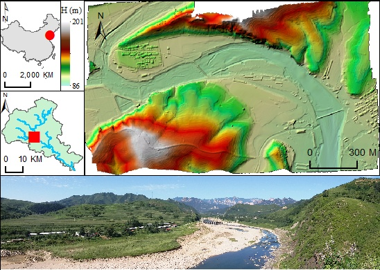
The study area is located at the Xiaobangshuiya Village (40°7′21″N; 119°34′10″E), adjacent to the Qinhuangdao National Geopark, and about 23 km northwest of Qinhuangdao City, Hebei Province, China (Figure 1a). The village is situated at the middle reach of Dashi River, which flows from northwest to southeast into the Bohai Sea with a length of 70 km and drains an area of 600 km2 (Figure 1b). The study valley is about 1.7 km in length and 1.1 km in width, covering an area of about 1.9 km2. The elevation of the valley varies between 86 m to 200 m above-sea-level, creating a total elevation range of ~ 120 m (Figure 1c). The study area exhibits a typical mountain valley topography characterized by slopes up to 70° (mean slope: 25°), which offers an opportunity to test the performance of UAS-based SfM over a complex terrain setting.
The geology of the valley comprises Quaternary alluvium and river terrace sand and gravel overlying the middle-late Jurassic Tiaojishan Formation. In this area, the Tiaojishan Formation bedrock consists of purple-red intermediate-basic volcanic and pyroclastic rocks [27]. The bedrock widely outcrops in the riverbed and the walls of the valley. There are no active faults within the study reach. The Dashi River is a mountainous intermittent river with great variability in flow because of seasonal precipitation. The water level during normal river flow period is between 0.5 m and 1.0 m, which can rise by 3 m to 6 m in the summer flood season [28]. The Dashi River in the study area has a strongly meandering character, running from the southwest to the northeast, and then to the south. As a result of the lateral erosion, the bedrock cliffs are formed in the concave bank, with heights up to 70 m and 40 m in the north and south bank, respectively. Accordingly, the river floodplains are developed in the convex bank due to the lateral accumulation. Some of the higher surfaces are fragmented and incised by fluvial erosion (Figure 1c). The width of the floodplain varies between 50 m to 390 m. Due to intermittent uplifts of the crust, multi-level river terraces were developed. Although most of them have now been transformed into roads, villages, and permanent arable land, several terraces can still be clearly identified in the DSM and in the field (Figure 1c,d). Land use within the study area is dominated by farmland, with some scrubland and rural settlements. Corn is the largest agricultural crop grown in this area.
Because of the representative features of fluvial geomorphology and well-preserved outcrops of middle Jurassic extrusive rocks, the study area has become an important field training site for students of geoscience-related majors [29]. Each summer, thousands of students from over 20 universities/colleges around China visit the study site to finish their field courses.
3. Materials and Methods
3.1. UAS Image Acquisition Over Complex Terrains and Ground Data Collection
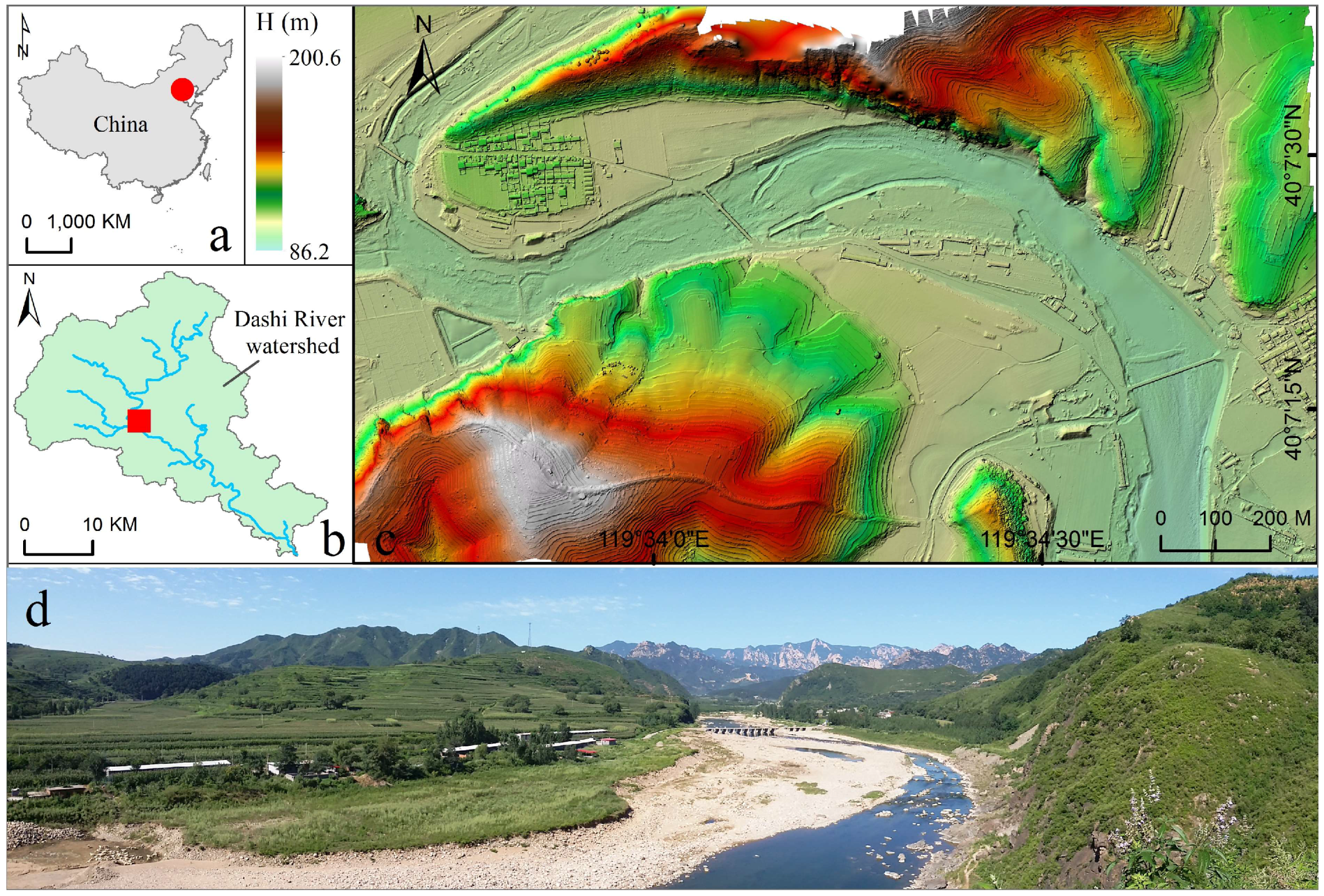
The UAS platform used is a small quadcopter, Phantom 4p by DJI (DJI Technologies, Shenzhen, China), with an integrated consumer-grade camera (Figure 2a). This portable UAS weighs less than 1.4 kg with a wingspan of 350 mm. The integrated camera featured a 35 mm equivalent (84° FOV) f/2.8-f/11 autofocus lens and a 1-inch type CMOS sensor of 20 megapixel (MP). The camera is mounted on to a 3-degree of freedom gimbal to maintain the nadir orientation during the image acquisition. The quadcopter has an onboard navigation system composed of an inertial measurement unit (IMU), altimeter, GPS, compass, and GPS-enabled autopilot. The UAS is controlled with an external tablet PC and remote control, which allows autonomous flights through waypoints predefined by the mission planning software package.
Since the area under investigation is relatively large and topographically complex, it is not possible to acquire the images with enough overlapping using a quadcopter by the conventional approach. Hence, we proposed an image acquisition approach for such complex settings, which involved the creation of sub mapping units to minimize the actual flight height variations above the ground, and the utilization of multiple batteries within a smart management mission planning software to extend the survey area. In this work, UAS aerial images were acquired under the leaves-off season on 28 March 2017 to ensure sparse, dormant vegetation. Conditions were clear and sunny, and wind speed was less than 7.0 m/s at the data collection time. The study valley was divided into two mapping units. As a result, the elevation variation was reduced from 120 m for the entire valley to 50 m and 60 m for each of the mapping unit, hence ensuring sufficient overlaps of acquired images. Two flights of parallel flight-lines orienting east-west were designed, which were at 150 m and 120 m above-ground-level (AGL), covering areas of 0.9 km2 and 1.0 km2, respectively (Figure 2b). For both flights, the speed was set to 10 m/s, and the across- and along-track overlaps set to 70% and 80%, respectively. The quadcopter took off at around the center of each flight unit to achieve the optimum usage of batteries, which yielded 7 and 8 flight lines, with a total flying time of 40 and 45 min, respectively (Figure 2b). The flight is planned via third-party software, that is, Map Pilot for DJI, featured by smart battery management function [30]. Although the quadcopter has a battery life of 30 min, an overhead of 9 min is usually left to safely land the UAS, and another 2 min is taken to travel from the takeoff to the start point. Net battery life of 19 min is available for image acquisition. Thus, three batteries are required for each of the flight. As a result, 516 and 594 geotagged images were acquired for each of the flights during 9:45 a.m. and 11:55 a.m., with Ground Sample Distances (GSD) of approximately 4.43 cm/pix and 3.54 cm/pix, respectively.
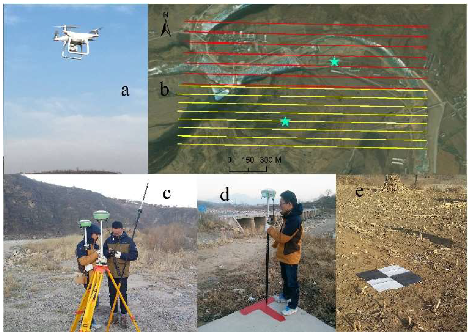
To produce orthomosaics and DSM, 19 ground targets were placed prior to the flight to serve as GCPs. The targets were either marked with red paint on roadsides (7 points) or 1 × 1 m painted canvas over farmlands (12 points) (Figure 2d,e), which are clearly visible in images (Figure 3b,c). The coordinate of each GCP was recorded by a survey grade dual-frequency RTK (real-time kinematic) GPS, composed of a base station and a rover (Figure 2c,d). The instrument has a manufacturer’s stated accuracy specification of ±1 cm + 1 ppm RMS horizontal, and ±2 cm + 1 ppm RMS vertical, which were confirmed with our repeatability tests. To assess the vertical accuracy of final DSM, independent field checkpoints were also surveyed as GTPs (Ground Truth Points). GTPs were collected as much as possible, distributed from the lowest riverside to the hilltop, accounting for all the elevations of the study valley. GTP recorded on the farmland surface must be performed with care since the GPS pole easily penetrates the soil for a few centimeters. In this work, a thin flat base was used with the pole to avoid this. As a result, a total of 196 GTPs were collected. All the points were measured in WGS84/ETRF2000 reference system, as shown in Figure 3a.
3.2. SfM Photogrammetry Workflow
Agisoft PhotoScan 1.3.0 (Agisoft LLC, St. Petersburg, Russia) was used to produce the DSM and orthomosaics from the images obtained by the two flights. PhotoScan is capable of processing images from different flying altitudes, and the final products have an average GSD value of the input images. To handle these massive data, PhotoScan was configured to run on a computer cluster, composed of a server and three hosts that were connected by a gigabit network (Table 1). In such a configuration, multiple PhotoScan instances running on different processing nodes can work on the same task in parallel, significantly reducing the total processing time [31]. The workflow regarding image processing of this work is briefly described below, and parameters were chosen based on test-and-trial (Table 2).
The workflow started with an image alignment stage. The alignment was done by detecting tie points within images and matching them based on their local neighborhood. PhotoScan uses a proprietary algorithm similar to the widely used scale-invariant feature transform (SIFT) [32] but slightly modified for higher alignment quality. The resulting sparse point cloud comprised of 3.85 million points for a density close to 15.4 point/m2. Meanwhile, the internal and external camera parameters were solved as well. However, these parameters are prone to some errors that can lead to non-linear deformations of the final model [33], and hence needed to be optimized. The second step of optimization involved two stages. First, the sparse point cloud was manually edited by removing obvious outliers and mislocated points. Second, 19 GCPs were used to georeference the model as well as optimize the camera parameters by minimizing the errors between the modeled locations and the measured ones; hence, there was no need to pre-calibrate the cameras and lens optics. The third step, dense point cloud building, was based on the optimized camera positions. Pair-wise depth maps were computed for each image using an MVS algorithm and then combined into a final dense point cloud. The MVS operates on pixel values rather than features and hence enables the fine details of the terrain to be constructed [34]. The resultant dense cloud comprised of about 1.72 billion points, corresponding to a density of 690 points/m2, which was then subject to some edition prior to proceeding to 3D mesh model generation to remove the most obvious point outliers. The fourth step, DSM and orthomosaic generation, was undertaken by converting the dense cloud to a triangulated surface mesh and calculating a texture atlas for the model. The mesh was further processed to a georeferenced DSM and orthomosaic by the projection of the images onto the surface.
3.3. Accuracy Assessment
The accuracy of DSM was evaluated by both GCPs and GTPs. After optimizing the photogrammetric network from the distribution of the GCPs, a residual error and a root mean square error (RMSE) were calculated for each point in both projection and pixel units. However, these statistics only show how well PhotoScan is fitting the data to the GCPs. In order to assess the accuracy of DSM in a more objective manner, GTPs independent of DSM generation were used. For these points, elevations were calculated from the DSM by the bilinear interpolation and then compared to the measured elevations. The statistics of vertical differences (dH) were calculated and analyzed, including mean, median, standard deviation (Stdev), RMSE, and mean absolute difference (MAD). The distribution of dH was obtained as well.
3.4. River Terrace Mapping and Analysis
Prior to the mapping, a morphological definition of river terraces is required so that all traces of ancient floodplains preserved until the present can be detected. The definition relies on an extended concept that river terraces are defined as low relief, quasi-planar areas capped by alluvium, and proximal to the modern river channel. Based on this definition, the method proposed by Clubb et al. [9] was employed to detect river terraces in this work. It was selected because it can replicate the extended concept as closely as possible by using two metrics, including elevation compared to the nearest channel, and local gradient. In addition, the previous results showed that the method can successfully extract terrace features compared to the field-mapped data, and is most accurate in areas where there is a contrast in slope between the feature of interest and the surrounding landscape, such as confined valley settings [9]. The two metrics can be readily calculated from the DSM after the pre-processing and channel extraction. Some morphological units of other origins (e.g., agricultural terraces) may be also included using this method, which were excluded by field check campaigns. The identified river terraces were further classified according to their elevations above the modern river channel. All the processes were performed using the ArcGIS 10.2 (ERSI, Redlands, CA., USA).
4. Results
4.1. DSM and Orthomosaic
A total of 1100 images were used to produce the DSM and orthomosaic. It took the computer cluster approximately 48 hours for the processing, including computational processing time and interactive adjustments. The output datasets had a uniform pixel resolution of 3.8 cm after accounting for the effects of mosaicking and orthorectification processes, as shown in Figure 1c and Figure 3a. A qualitative assessment was made of the orthomosaic, which revealed that cut lines were not detectable and image color balancing was good. The exceptions were a few areas in the boundary where the overlap was not sufficient, and gaps were created. Since the images were taken in the leaves-off season, the generated DSM provides a good representation of the terrain, making it well suited for the recognition of landforms. For example, terrace treads can be visually identified by a distinct change in slope from the terrace riser to approximately planar former floodplain surfaces (Figure 1c). The agriculture terraces on the hillside can also be observed from the DSM (Figure 1c).
4.2. DSM Accuracy
The error statistics generated using GCPs are summarized in Table 3a. The accuracy statistics suggested that the georeferencing had a total RMSE value of 3.34 cm. The total x and y RMSE values were 2.02 and 2.24 cm, respectively, which were less than the image resolution. Compared to other remote sensing data, this is a relatively small horizontal error, especially when considering a large number of images of different scales used to create the orthomosaic. The vertical RMSE value was 1.14 cm. The mean reprojection error (MRE) is less than 0.4 pixel. This error can be seen as a proxy of geometric accuracy of the bundle adjustment as it uses the interior and exterior camera orientation parameters. These accuracy values seem quite satisfactory but may be misleading. These indicators only provide an assessment of the internal coherence of the photogrammetric process and of the quality of alignment, and, consequently, of the depth reconstruction from which are derived the dense point clouds. As such, the vertical accuracy of the DSM is more objectively assessed from GTPs independent of the dataset generation, as listed in Table 3b.
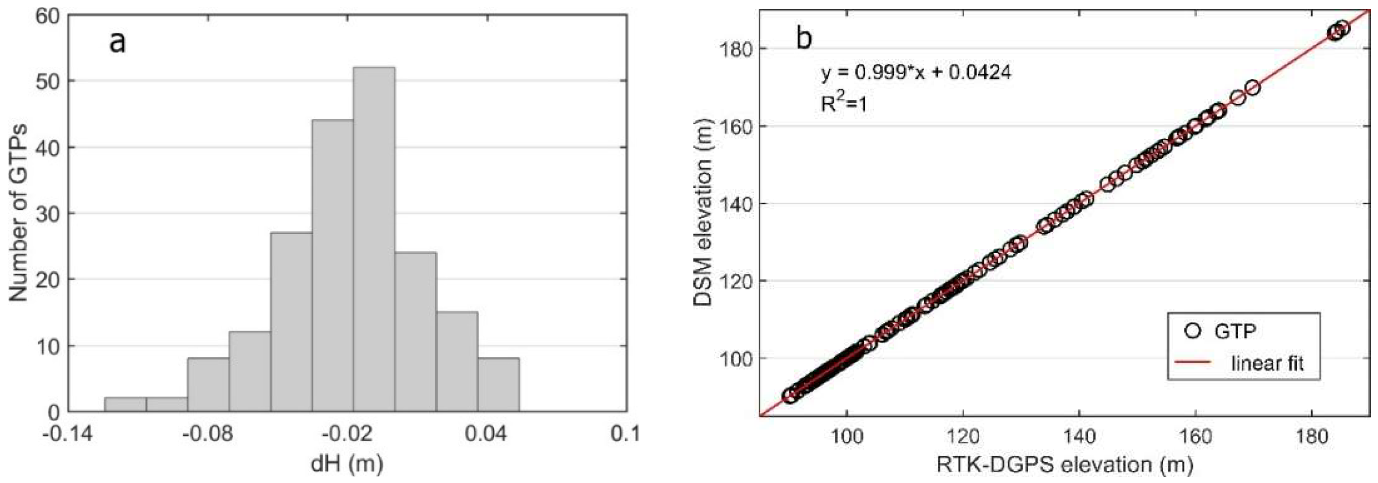
Figure 4a shows the distribution of dH, which appears to be nearly normal. Positive values indicate that the elevations of points on the DSM surface are greater than the corresponding elevations of GPS points, and vice versa. In the histogram, the overall accuracy of DSM was very satisfactory with a large proportion of GTPs centered on a mean error of −1.8 cm and a median of −1.7 cm (Table 3b). It indicated that the generated DSM was slightly lower than the real terrain. The MAD and the RMSE were similar with values of 2.9 and 3.1 cm, respectively, revealing an accurate reconstruction of the valley topography (Table 3b). We calculated 58.7% of dH values within a ±3 cm interval, 90.3% within ±6 cm, and 98.5% within ±9 cm, while only 1.5% exceeds the interval of ±9 cm. The greatest difference value is −12.4 cm. Figure 4b presents GTP elevations estimated from the DSM as a function of GTP elevations obtained by RTK-GPS. The figure indicates a perfect linear fit with a coefficient of determination (R2) of 1, demonstrating that there are no major outliers present, and no systematic offset between the DSM and GTP observations.
4.3. River Terraces
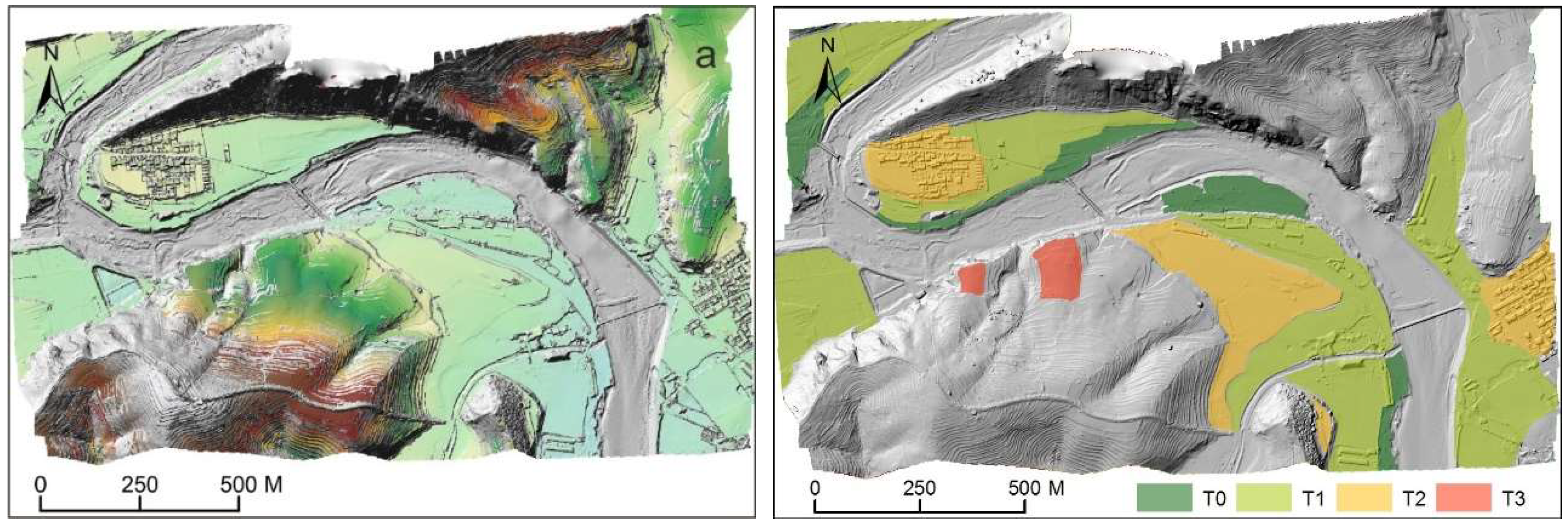
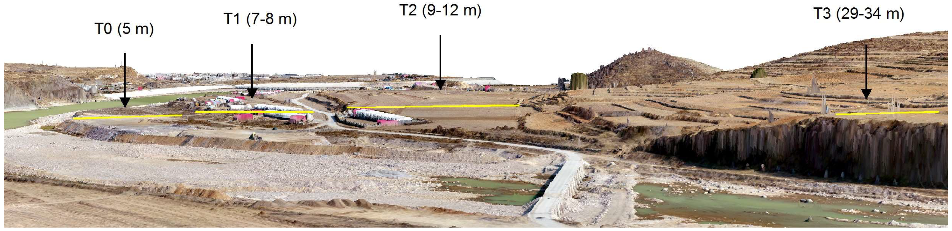
After applying the terrace extraction method to the generated DSM, a map of potential terrace areas (PTAs) was obtained, as shown in Figure 5a. The presence and distribution of PTAs were generally consistent with the extent of terraces from a visual inspection of shaded DSM. The results were further validated through the fieldwork. Most of the PTAs were confirmed due to the observation of natural planation surfaces or fluvial sediments. Some of the PTAs were excluded since they correspond to anthropic agricultural terraces. The validated river terrace map is shown in Figure 5b. Based on tread height distributions, river terraces were classified into four categories, including 5 m (T0), 7–8 m (T1), 9–12 m (T2), and 29–34 m (T3) above the present bankfull level. The characteristics of these river terraces are briefly described below.
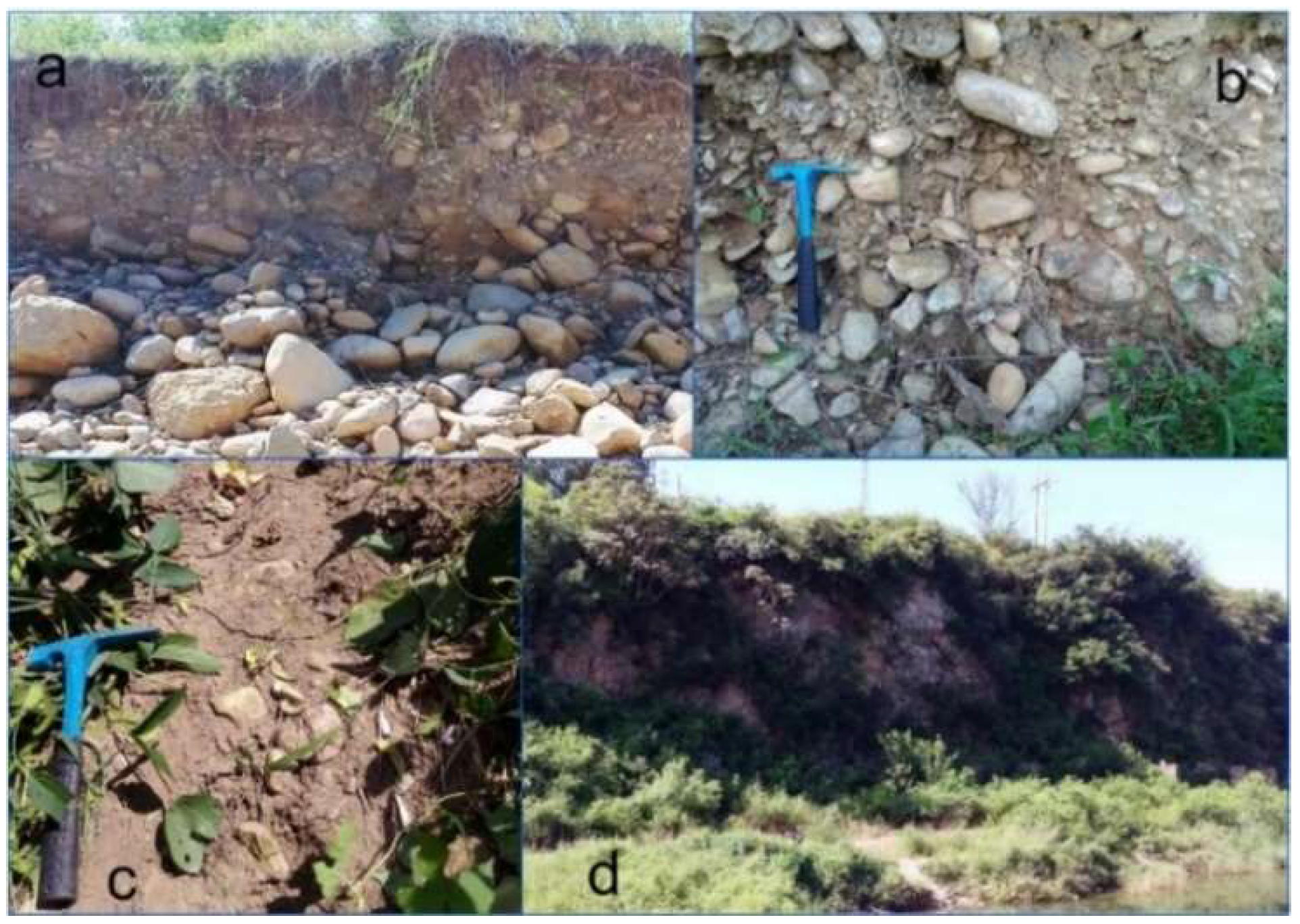
T0 is approximately 5 m above the bankfull and closely distributed to the river bed. Field observations of characteristics of T0 risers indicated a significant proportion of large rounded and often pitted cobble to boulder-sized clasts, within a matrix of sand and gravel (Figure 6a). Modern deposition results indicated that T0 is part of the active floodplain, and these surfaces are the high floodplain, and therefore, not considered as river terraces. T1 treads are common throughout the study area in height from 7 to 8 m above bankfull. The extent of these treads is limited to the near-channel environment, and these terraces are typically found on the inside of meander bends, or in a narrow band parallel to the present channel. It has been transformed into rural settlements and roads. T2 terrace treads are found throughout the study valley, and heights of these treads are between 9 and 12 m above bankfull. They are expressed as elongated benches parallel to and above the river channel (Figure 5b). It covers the largest area underlain fluvial deposits. The terrace has been transformed into permanent farmland. At some locations, terraces within this height range are characterized by medium to large boulders exposed in terrace risers (Figure 6b) or at the treads (Figure 6c). T3 terrace is bedrock strath terrace and overlain by alluvium of variable thickness, with a height of 29–34 m above bankfull (Figure 6d). The terrace is discontinuous as it has been eroded over time (Figure 5b). The bedrock is frequently exposed along the erosion gullies. The terrace remnants have been transformed into farmlands at different elevation levels, forming multi-level agricultural terraces (Figure 2b).
5. Discussion
5.1. Mapping of Complex Terrains Over Relatively Large Spatial Extents
Mapping of complex terrains over large spatial extents is not an easy thing. First, it requires the UAS to fly for a considerable amount of time and need little space to take off or land, which pose challenges for most UASs. Although the fixed-wings have longer flight durations thus enabling larger survey areas, they require considerable open spaces for take-off and landing, which are usually unavailable over complex terrains. The rotary ones can vertically take off and land, however, they can only survey limited areas [18]. For mapping of the study valley, a rotary quadcopter was selected as it can take off and land almost anywhere, making it well suited to fly in rugged and limited terrains [19]. Although the 1.9 km2 coverage of the study valley is far beyond the limit of the quadcopter, the survey was made possible by using multiple batteries along with a mission planning software. In addition to creating the flight path, Map Pilot for DJI also features smart management of multiple batteries [30]. During the survey, the quadcopter was automatically returned home once the user’s battery timer ran out, the point of abandonment was recorded, and the quadcopter would pick right back up the point with the fresh battery and continued the remaining mission. With this feature, survey areas of Phantom 4p could be significantly extended, making it capable of mapping complex or inaccessible terrains of relatively large spatial extents where fixed-wings or traditional survey methods would be unfeasible or unsafe.
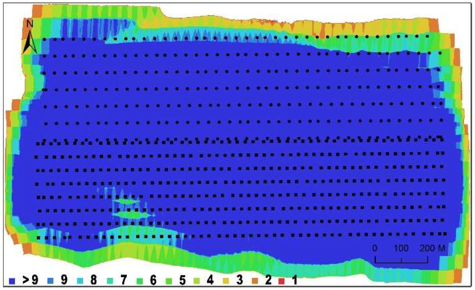
Second, sufficient overlap among images is hard to achieve over highly undulating terrains since the actual flight height above the ground is quite variable. The overlap is of key importance for producing high-quality DSMs. It has been reported that DSM accuracy improves as the overlap increases due to a better estimation of the image block orientation parameters [35]. To ensure sufficient overlap, two mapping units were created with different flight altitudes orienting east-west in this study (Figure 2b), which roughly correspond to the trending of topography. Under such a flight plan, elevation variations of the two units are significantly reduced. For mapping of even more complex terrains, more mapping units may be created to minimize the actual flight height variations above the ground. In this work, the same across- and along-track overlaps of 70% and 80%, respectively, were used for the two flights because the SfM algorithms are capable to automatically process images of different overlaps [13]. In addition, the overlap values were large enough for SfM photogrammetry, which would strengthen the block geometry. With the proposed mission planning approach, an adequate image overlapping across all locations was guaranteed, as shown in Figure 7. Despite the huge topographic variation, the effective overlap of >9 images per point was achieved for most of the study area. An exception occurred at the lower left of the study area, where two big radio transmission towers (about 60 m in height) are standing on the top of the hill, disrupting image matching with occlusion. In recent years, some advanced mission planning software allows UAS to acquire images with the same spatial resolution by following the terrain morphology. This is especially effective in cases with large variations in terrain elevation as most of this software utilize the 30 m SRTM (Shuttle Radar Topography Mission) DEM for terrain following capabilities. In future surveys, this kind of utility should be exploited to acquire images with uniform resolutions.
Third, GCP setup and image processing need to be additionally addressed as they are the most time-consuming steps in the mapping of complex terrains over relatively large spatial extents. For example, it took about half a day for deploying and measuring the 19 GCPs in the field, not mentioning the time needed for identification of GCPs within the imagery. Recently, the direct georeferencing of UAS images are very popular, which enables imagery to be georectified without the need for GCPs [36]. It simplifies the data collection process, making the use of UASs more cost-effective and time efficient. Hence, direct georeferencing should be considered regarding the mapping of complex terrains over large spatial extents. The time requirements for image processing depend on the degree of detailedness and the number of images. For the processing of massive data with a high detail level, cluster computers with multiprocessor and GPU acceleration are strongly recommended.
Overall, the results demonstrated that the proposed workflow of mapping topographically complex terrains of large spatial extents using a quadcopter is reliable. Our work provides the guidelines for UAS surveys under such complex conditions, therefore, promoting quick and cost-effective landform mapping applications in remote or poorly accessible areas.
5.2. Spatial Resolution and Vertical Accuracy
Landform mapping strongly relies on the details of digital terrain. With careful mission plan, flight execution and image processing, we obtained a dense cloud of 690 points/m2 for the highest reconstruction quality. It is almost the same density as TLS point clouds (i.e., a mean density of 760 points/m2 [24]), and denser than most of LiDAR point clouds (i.e., a density of 35 points/m2 [37]). The dense cloud resulted in a 3.8-cm ultrahigh-resolution DSM. The effective DSM resolution is largely determined by the density of point cloud, while that of the orthomosaic depends entirely on the resolution of original images. Hence, the 3.8-cm resolution for orthomosaic may be an artificial resolution associated with the interpolation in PhotoScan, as the GSDs of the input image are 3.54 cm/pix and 4.43 cm/pix, respectively. It is noted that for landform mapping applications, the spatial resolution of DSM should match the scale of landform under investigation. In this work, the generated ultrahigh-resolution DSM seems too detailed for the detection of large-scale river terraces. A resampling process may be applied to derive a coarser DSM, which will be especially effective when a complicated river terrace detection algorithm is employed.
The accuracy of topographic data is critical for landform mapping. Despite the complex terrain, a vertical RMSE of 3.1 cm was achieved over the study valley. The vertical accuracy is superior to that of typical airborne LiDAR surveys (15 cm elevation RMSE [38]) and even better than the accuracy of TLS (5 cm elevation RMSE [39]). Meanwhile, compared to LiDAR surveys, the cost of the proposed method is significantly reduced. The vertical accuracy achieved in this work is also comparable with the results obtained from other similar UAS studies conducted under different geomorphologic settings (Table 4). For example, our results exceed those reported by Long et al. [22], Gonçalves et al. [24], and Tonkin et al. [18] of 17 cm, 12 cm, and 51.7 cm vertical RMSE, respectively, and are similar to those reported by Gonçalves et al. [20] of 2.7–4.6 cm vertical RMSE.
The high accuracy of DSMs obtained in this work could be attributed to several reasons, including the proper deployment of GCPs, the season of image acquisition, as well as sufficient image overlap. The number and spatial distribution of GCPs have a strong influence on the accuracy of DSMs derived from UAS photogrammetry. Several previous studies have concluded that DSM accuracy improves with the increase of GCPs until a certain density of GCPs is reached [23,40,41,42]. In our UAS dataset, 19 GCPs were deployed across the study area, resulted in a mean error of 0.34 pixel for the coordinates of these points by multi-ray intersection. It is likely that the number and distribution of GCPs were sufficient to properly parameterize the 3D model during bundle adjustment. The presence of vegetation is another known cause of poor accuracy in UAS derived DSMs. The vegetation may obscure or obstruct line-of-sight of actual ground level and disrupt image matching with shadow and occlusion [43]. We suspect that the low vertical accuracies reported by Tonkin et al. [18] might be related to the influence of vegetation, where the vertical error is found particularly pronounced around trees, and in areas vegetated with heather. Therefore, it is suggested that the UAS survey should be made during leave-off seasons to increase the accuracy of DSM, as well as capture relief features. The image overlap can also impact the DSM accuracy as discussed in the previous section. The high overlapping can result in an accuracy improvement in the point cloud extraction, which contributes to the high accuracy of DSM. However, the major error source in this work is likely to be the 2 cm vertical accuracy of RTK-GPS, as the obtained 3.1 cm accuracy is not much greater than the measurement accuracy.
Overall, our results suggested that the low-cost UAS-based SfM photogrammetry can deliver highly accurate topographic information over complex valleys. In addition to landform mapping, multi-temporal UAS imagery may also be used to measure topographic changes associated with landform morphodynamics, such as the morphological changes of river channel bar in response to a flood event [44].
5.3. Terrace Extraction
After validation, it was accepted that there are three levels of river terraces, presenting a relatively good continuity along the studied valley. The obtained results were compared with previous works concerning the terraces of the study area [28,29]. These authors described three levels of river terraces located at approximately 3–5 m, 12 m, and 21–25 m above the present bankfull level. Our results are generally consistent with the findings of the previous studies. However, they did not give the detailed river terrace map. Additionally, it is interesting to note that three levels of wave-cut platforms and cliff notches located at the similar levels as the river terraces were also documented in this region [29], suggesting that the amounts of tectonic uplifts were comparable to those derived from river terrace sequences.
The employed methodology may have several advantages over previous mapping techniques. Compared with field mapping [5], the high-resolution DSM is helpful when dealing with less developed or severely eroded terraces whose detection could have been missed as a synoptic view is lacking when standing in the terrace. Compared with automatic river terrace mapping [6,7,8,9], which were mainly based on relatively coarse DEMs, UAS-SfM mapping allows more accurate identification of vertical offsets of terrace levels. On this basis, dating samples can be taken for age estimation using optically stimulated luminescence technique, which may provide important information on river downcutting rates during different periods. Although UAS-SfM mapping can provide a detailed and overall view of river terraces, it is never a replacement for field observations as it cannot distinguish river terraces from some other planar features as shown in our case. Therefore, the integration of both methods is suggested to obtain a more complete and accurate river terrace map. In addition, the high-resolution UAS-SfM datasets allow the detailed 3D construction of the area under investigation [15], which greatly facilitates the landform detection and interpretation. For example, Figure 8 is the 3D representation of the study valley, which clearly shows the array of river terraces, revealing that the Dashi River has gone through downcutting in several periods. The chronological order of terraces can be easily inferred from their distances to the river as well.
A key goal for the Earth surface research community is to develop fully automated methods of feature extraction from high-resolution DEMs to avoid expensive and time-consuming field mapping [9]. The low-cost UAS based SfM photogrammetry along with a terrace detection algorithm employed in this paper represents the first step towards this goal. The former demonstrates the capabilities of this technique for producing fine-scale DSMs over complex terrains. The latter attempts to meet some of these research needs by allowing the statistical determination of the thresholds for terrace extraction. Meanwhile, with ever increasing spatial resolutions of DSMs, application of object-based image analysis (OBIA) for landform identification has received much attention [45]. OBIA allows for the automatic mapping of features that are invariant and accurate in resembling the geomorphologists’ views of landforms. Several authors have underlined the superiority of the OBIA through mapping practices of a variety of landforms, including glaciovolcanic landforms [46], drumlins [47], and gully-affected areas [48]. In the future, attempts should be made to develop the OBIA framework for river terrace detection based on the generated DSMs.
6. Conclusions
This study is, to our knowledge, the first one to evaluate the performance of low-cost UAS-based SfM photogrammetry for terrace mapping over a complex terrain setting with a relatively large spatial extent. For a survey of such a complex area using a quadcopter, an image acquisition approach was proposed, which involved the creation of sub mapping units to ensure sufficient overlaps of acquired images, and the utilization of multiple batteries within a smart management mission planning software to extend the survey area. The study was carried out over the 1.9 km2 valley of Dashi River, Qinhuangdao, China. As a result, a 3.8 cm resolution orthomosaic and DSM were generated from a total of 1100 images acquired from the two mapping units. The vertical accuracy of DSM was assessed against 196 independent checkpoints measured with an RTK GPS, which showed that the RMSE and MAE are 3.1 cm and 2.9 cm, respectively. Based on the generated DSM, a high-level floodplain and three level river terraces were identified, which were 5.0 m (T0), 7–8 m (T1), 9–12 m (T2), and 29–34 m (T3) above the present bankfull level. The field validation confirmed that most of the delineated terraces correspond to terrace remnants.
In summary, this study highlighted that the highly accurate DSM of centimeter-level resolution could be obtained over complex terrain settings using the low-cost UAS-based SfM photogrammetry, competitive with those delivered using more expensive laser scanning. The generated DSM is particularly suitable for the quick and cost-effective mapping of river terraces. This work provides the workflow for the production of highly accurate datasets under such complex conditions and thus promotes landform mapping applications in remote or poorly accessible areas. Additionally, there are several advantages of UAS-based SfM photogrammetry, including low-cost, high efficiency, high vertical accuracy, centimeter-level resolution, and large spatial extent. Future work will focus on the development of OBIA framework for river terrace detection using these SfM-generated DSMs.
Author Contributions
H.L. conceived and designed the experiments, and wrote the manuscript. L.C. carried out image processing and analyzed the data, as well as provided constructive discussions. Z.W. and Z.Y. conducted the UAS survey as well as GCP and GTP measurements in the field. All authors read and approved the final manuscript.
Funding
This research was funded by the National Natural Science Foundation of China, grant numbers J1310038, 41201429 and 41391240191.
Acknowledgments
The authors wish to thank Chu Daoliang and Shen Tianyi from the school of earth sciences, China University of Geosciences for their assistance in the field check campaign. We would also like to thank the anonymous reviewers for their constructive comments that significantly improved our manuscript.
Conflicts of Interest
The authors declare no conflict of interest.
References
- Pazzaglia, F.J.; Gardner, T.W. Fluvial terraces of the lower Susquehanna River. Geomorphology 1993, 8, 83–113. [Google Scholar] [CrossRef]
- Limaye, A.B.; Lamb, M.P. Numerical model predictions of autogenic fluvial terraces and comparison to climate change expectations. J. Geophys. Res. Earth 2016, 121, 512–544. [Google Scholar] [CrossRef] [Green Version]
- Pederson, J.L.; Anders, M.D.; Rittenhour, T.M.; Sharp, W.D.; Gosse, J.C.; Karlstrom, K.E. Using fill terraces to understand incision rates and evolution of the Colorado River in eastern Grand Canyon, Arizona. J. Geophys. Res. Earth 2006, 111, F02003. [Google Scholar] [CrossRef]
- Bridgland, D.; Westaway, R. Climatically controlled river terrace staircases: A worldwide Quaternary phenomenon. Geomorphology 2008, 98, 285–315. [Google Scholar] [CrossRef] [Green Version]
- Meikle, C.; Stokes, M.; Maddy, D. Field mapping and GIS visualisation of Quaternary river terrace landforms: An example from the Rio Almanzora, SE Spain. J. Maps 2010, 6, 531–542. [Google Scholar] [CrossRef]
- Demoulin, A.; Bovy, B.; Rixhon, G.; Cornet, Y. An automated method to extract fluvial terraces from digital elevation models: The Vesdre valley, a case study in eastern Belgium. Geomorphology 2007, 91, 51–64. [Google Scholar] [CrossRef]
- Passaro, S.; Ferranti, L.; de Alteriis, G. The use of high-resolution elevation histograms for mapping submerged terraces: Tests from the Eastern Tyrrhenian Sea and the Eastern Atlantic Ocean. Quatern. Int. 2011, 232, 238–249. [Google Scholar] [CrossRef]
- Stout, J.C.; Belmont, P. TerEx Toolbox for semi-automated selection of fluvial terrace and floodplain features from LiDAR. Earth Surf. Proc. Landf. 2014, 39, 569–580. [Google Scholar] [CrossRef]
- Clubb, F.J.; Mudd, S.M.; Milodowski, D.T.; Valters, D.A.; Slater, L.J.; Hurst, M.D.; Limaye, A.B. Geomorphometric delineation of floodplains and terraces from objectively defined topographic thresholds. Earth Surf. Dyn. Discuss. 2017, 5, 369–385. [Google Scholar] [CrossRef]
- Li, H.; Zhao, J.Y. Evaluation of the Newly Released Worldwide AW3D30 DEM Over Typical Landforms of China Using Two Global DEMs and ICESat/GLAS Data. IEEE J. Sel. Top. Appl. Earth Obs. Remote Sens. 2018, 11, 4430–4440. [Google Scholar] [CrossRef]
- Wilson, J.P. Digital terrain modeling. Geomorphology 2012, 137, 107–121. [Google Scholar] [CrossRef]
- Ullman, S. The interpretation of structure from motion. Proc. R. Soc. B Biol. 1979, 203, 405–426. [Google Scholar] [CrossRef] [Green Version]
- Smith, M.; Carrivick, J.; Quincey, D. Structure from motion photogrammetry in physical geography. Prog. Phys. Geog. 2016, 40, 247–275. [Google Scholar] [CrossRef]
- Javernick, L.; Brasington, J.; Caruso, B. Modeling the topography of shallow braided rivers using Structure-from-Motion photogrammetry. Geomorphology 2014, 213, 166–182. [Google Scholar] [CrossRef]
- James, M.R.; Robson, S. Straightforward reconstruction of 3D surfaces and topography with a camera: Accuracy and geoscience application. J. Geophys. Res. Earth 2012, 117, F03017. [Google Scholar] [CrossRef]
- Nebiker, S.; Annen, A.; Scherrer, M.; Oesch, D. A light-weight multispectral sensor for micro UAV–Opportunities for very high resolution airborne remote sensing. ISPRS Arch. 2008, 37, 1193–1199. [Google Scholar]
- Turner, D.; Lucieer, A.; Watson, C. An automated technique for generating georectified mosaics from ultra-high resolution unmanned aerial vehicle (UAV) imagery, based on structure from motion (SfM) point clouds. Remote Sens. 2012, 4, 1392–1410. [Google Scholar] [CrossRef]
- Tonkin, T.N.; Midgley, N.G.; Graham, D.J.; Labadz, J.C. The potential of small unmanned aircraft systems and structure-from-motion for topographic surveys: A test of emerging integrated approaches at Cwm Idwal, North Wales. Geomorphology 2014, 226, 35–43. [Google Scholar] [CrossRef] [Green Version]
- Immerzeel, W.W.; Kraaijenbrink, P.D.A.; Shea, J.M.; Shrestha, A.B.; Pellicciotti, F.; Bierkens, M.F.P.; De Jong, S.M. High-resolution monitoring of Himalayan glacier dynamics using unmanned aerial vehicles. Remote Sens. Environ. 2014, 150, 93–103. [Google Scholar] [CrossRef]
- Gonçalves, J.A.; Henriques, R. UAV photogrammetry for topographic monitoring of coastal areas. ISPRS J. Photogramm. Remote Sens. 2015, 104, 101–111. [Google Scholar] [CrossRef]
- Cook, K.L. An evaluation of the effectiveness of low-cost UAVs and structure from motion for geomorphic change detection. Geomorphology 2017, 278, 195–208. [Google Scholar] [CrossRef]
- Long, N.; Millescamps, B.; Guillot, B.; Pouget, F.; Bertin, X. Monitoring the Topography of a Dynamic Tidal Inlet Using UAV Imagery. Remote Sens. 2016, 8, 387. [Google Scholar] [CrossRef]
- Gindraux, S.; Boesch, R.; Farinotti, D. Accuracy assessment of digital surface models from unmanned aerial vehicles’ imagery on glaciers. Remote Sens. 2017, 9, 186. [Google Scholar] [CrossRef]
- Gonçalves, G.R.; Pérez, J.A.; Duarte, J. Accuracy and effectiveness of low cost UASs and open source photogrammetric software for foredunes mapping. Int. J. Remote Sens. 2018, 39, 5059–5077. [Google Scholar] [CrossRef]
- Gómez-Gutiérrez, Á.; Schnabel, S.; Berenguer-Sempere, F.; Lavado-Contador, F.; Rubio-Delgado, J. Using 3D photo-reconstruction methods to estimate gully headcut erosion. Catena 2014, 120, 91–101. [Google Scholar] [CrossRef]
- Hemmelder, S.; Marra, W.; Markies, H.; De Jong, S.M. Monitoring river morphology & bank erosion using UAV imagery—A case study of the river Buëch, Hautes-Alpes, France. Int. J. Appl. Earth Obs. 2018, 73, 428–437. [Google Scholar] [CrossRef]
- Liu, Y.; Kuang, H.; Peng, N.; Xu, H.; Zhang, P.; Wang, N.; An, W. Mesozoic basins and associated palaeogeographic evolution in North China. J. Palaeogeogr. 2015, 4, 189–202. [Google Scholar] [CrossRef] [Green Version]
- Wang, J.; Zhou, J.; Yang, X.; Chen, Z. Sedimentary characteristics and geneses of pebbly meandering river: A case from Dashihe River in Qinghuangdao Area. Earth Sci. 2018, 43, 277–286, (In Chinese with English abstract). [Google Scholar]
- Wang, J.S. Routes of geology cognition practice. In Teaching Guidebook of Beidaihe Geology Cognition Practice; Wang, J., Ed.; China University of Geosciences Press: Beijing, China, 2011; pp. 73–78. (In Chinese) [Google Scholar]
- Flying Multi-battery Missions. Drones Made Easy. Available online: https://support.dronesmadeeasy.com/hc/en-us/articles/206104736-Flying-Multi-Battery-Missions (accessed on 13 November 2018).
- Agisoft PhotoScan User Manual—Professional Edition, Version 1.4. Available online: http://www.agisoft.com/pdf/photoscan-pro_1_4_en.pdf (accessed on 5 December 2018).
- Lowe, D.G. Object recognition from local scale-invariant features. In Proceedings of the Seventh IEEE International Conference on Computer Vision, Kerkyra, Greece, 20–27 September 1999; pp. 1150–1157. [Google Scholar] [CrossRef]
- Carbonneau, P.E.; Dietrich, J.T. Cost-effective non-metric photogrammetry from consumer-grade sUAS: Implications for direct georeferencing of structure from motion photogrammetry. Earth Surf. Proc. Landf. 2017, 486, 473–486. [Google Scholar] [CrossRef]
- Verhoeven, G. Taking computer vision aloft—Archaeological three-dimensional reconstructions from aerial photographs with Photoscan. Archaeol. Prospect. 2011, 18, 67–73. [Google Scholar] [CrossRef]
- Rosnell, T.; Honkavaara, E. Point Cloud Generation from Aerial Image Data Acquired by a Quadrocopter Type Micro Unmanned Aerial Vehicle and a Digital Still Camera. Sensors 2012, 12, 453–480. [Google Scholar] [CrossRef] [PubMed] [Green Version]
- Turner, D.; Lucieer, A.; Wallace, L. Direct Georeferencing of Ultrahigh-Resolution UAV Imagery. IEEE Trans. Geosci. Remote Sens. 2014, 52, 2738–2745. [Google Scholar] [CrossRef]
- Yang, H.; Chen, W.; Qian, T.; Shen, D.; Wang, J. The Extraction of Vegetation Points from LiDAR Using 3D Fractal Dimension Analyses. Remote Sens. 2015, 7, 10815–10831. [Google Scholar] [CrossRef] [Green Version]
- Xhardé, R.; Long, B.F.; Forbes, D.L. Accuracy and limitations of airborne LiDAR surveys in coastal environments. In Proceedings of the Geoscience and Remote Sensing Symposium, Denver, CO, USA, 31 July–4 August 2006; pp. 2412–2415. [Google Scholar] [CrossRef]
- Hollenbeck, J.; Olsen, M.; Haig, S. Terrestrial laser scanning to support ecological research in the rocky intertidal zone. J. Coast. Conserv. 2014, 18, 701–714. [Google Scholar] [CrossRef]
- Tahar, K.N. An evaluation on different number of ground control points in unmanned aerial vehicle photogrammetric block. In Proceedings of the ISPRS 8th 3D GeoInfo Conference & WG II/2 Workshop, Istanbul, Turkey, 27–29 November 2013; pp. 93–98. [Google Scholar]
- Tonkin, T.N.; Midgley, G.N. Ground-control networks for image based surface reconstruction: An investigation of optimum survey designs using UAV derived imagery and structure-from-motion photogrammetry. Remote Sens. 2016, 8, 786. [Google Scholar] [CrossRef]
- Martínez-Carricondo, P.; Agüera-Vega, F.; Carvajal-Ramírez, F.; Mesas-Carrascosa, F.J.; García-Ferrer, A.; Pérez-Porras, F.J. Assessment of UAV-photogrammetric mapping accuracy based on variation of ground control points. Int. J. Appl. Earth Obs. 2018, 72, 1–10. [Google Scholar] [CrossRef]
- James, M.R.; Robson, S.; d’Oleire-Oltmanns, S.; Niethammer, U. Optimising UAV topographic surveys processed with structure-from-motion: Ground control quality, quantity and bundle adjustment. Geomorphology 2017, 280, 51–66. [Google Scholar] [CrossRef]
- Wang, Z.; Li, H.; Cai, X. Remotely Sensed Analysis of Channel Bar Morphodynamics in the Middle Yangtze River in Response to a Major Monsoon Flood in 2002. Remote Sens. 2018, 10, 1165. [Google Scholar] [CrossRef]
- Drăguţ, L.; Eisank, C. Object representations at multiple scales from digital elevation models. Geomorphology 2011, 129, 183–189. [Google Scholar] [CrossRef] [PubMed] [Green Version]
- Pedersen, G.B.M. Semi-automatic classification of glaciovolcanic landforms: An object-based mapping approach based on geomorphometry. J. Volcanol. Geotherm. Res. 2016, 311, 29–40. [Google Scholar] [CrossRef] [Green Version]
- Eisank, C.; Smith, M.; Hillier, J. Assessment of multiresolution segmentation for delimiting drumlins in digital elevation models. Geomorphology 2014, 214, 452–464. [Google Scholar] [CrossRef] [PubMed] [Green Version]
- D’Oleire-Oltmanns, S.; Marzolff, I.; Tiede, D.; Blaschke, T. Detection of gully-affected areas by applying object-based image analysis (OBIA) in the region of Taroudannt, Morocco. Remote Sens. 2014, 6, 8287–8309. [Google Scholar] [CrossRef]
Figure 1.
Geographical location of the study area in relation to (a) China (as indicated by red dot), and (b) Dashi River watershed (as indicated by a red square). (c) The color shaded digital surface model (DSM) and (d) panoramic photograph illustrating the topography and landscape of the study area. Flow is west to east and photo is taken downstream looking upstream.

Figure 2.
Unmanned Aerial Systems (UAS) aerial image acquisition and ground control points (GCP) collection setup. (a) Phantom 4p quadcopter at takeoff. (b) Flight lines of two flights (as shown by red and yellow color) and corresponding take-off/landing locations (as indicated by cyan stars). (c) Real-time kinematic (RTK) GPS base station setup. Examples of ground targets, (d) roadside painted targets and (e) 1 × 1 m painted canvas.

Figure 3.
The locations of ground control points (GCPs) and ground truth points (GTPs) overlaid on the generated orthomosaic of the study area (a), as well as GCP targets of red paint (b) and painted canvas (c) seen from the acquired images.
Figure 3.
The locations of ground control points (GCPs) and ground truth points (GTPs) overlaid on the generated orthomosaic of the study area (a), as well as GCP targets of red paint (b) and painted canvas (c) seen from the acquired images.

Figure 4.
DSM accuracy based on 196 GTPs. The histogram (a) shows the distribution of dH errors. The graph (b) shows the elevation estimate from the DSM as a function of the RTK-DGPS elevation.
Figure 4.
DSM accuracy based on 196 GTPs. The histogram (a) shows the distribution of dH errors. The graph (b) shows the elevation estimate from the DSM as a function of the RTK-DGPS elevation.

Figure 5.
The distribution of potential river terraces (a) and validated river terraces (b) overlaid on the shaded DSM of the study valley.
Figure 5.
The distribution of potential river terraces (a) and validated river terraces (b) overlaid on the shaded DSM of the study valley.

Figure 6.
Fieldwork validation of the potential terrace areas detected in the study river valley. (a) Riser of T0 floodplain adjacent to the modern river channel. (b) Riser of T2 terrace. (c) Fluvial gravels on T2 terrace tread. (d) A side view of T3 bedrock strath terrace, showing fluvial sediments on the bedrock.

Figure 7.
Camera locations and image overlaps. The legend indicates the number of overlapping images of that location.
Figure 7.
Camera locations and image overlaps. The legend indicates the number of overlapping images of that location.

Figure 8.
A 3D representation of the study area, illustrating the river terraces of different levels. The numbers in parentheses indicate the heights of terrace treads above the present bankfull level.
Figure 8.
A 3D representation of the study area, illustrating the river terraces of different levels. The numbers in parentheses indicate the heights of terrace treads above the present bankfull level.


Table 1.
Computer cluster setup for network processing.
| Node | CPU | RAM | GPU |
|---|---|---|---|
| Host1 | Intel i7 6900K | 32 GB DDR4 | 2×NVIDIA GeForce GTX1080 |
| 3.2 GHz, 8 cores | 2560 CUDA cores and 8 GB RAM | ||
| Host2 | AMD Ryzen 7 1800X | 16 GB DDR4 | NVIDIA GeForce GTX1080 |
| 3.6 GHz, 8 cores | 2560 CUDA cores and 8 GB RAM | ||
| Host3 | Intel i7 6700K | 16 GB DDR4 | NVIDIA GeForce GTX1060 |
| 4.0 GHz, 4 cores | 1280 CUDA cores and 6 GB RAM | ||
| Server | Intel i7 4790 | 16 GB DDR3 | NVIDIA Quadro 2000 |
| 3.6 GHz, 4 cores | 192 CUDA cores and 1 GB RAM |
CPU: central processing unit; RAM: random access memory; GPU: graphics processing unit.
Table 2.
Parameters used in PhotoScan software.
| 1. Photoalignment parameters | ||||
| Accuracy | Pair preselection | Point limit | ||
| High | Reference | 80,000 | ||
| 2. Optimization | ||||
| Camera accuracy | Marker accuracy | Projection accuracy | Tie point accuracy | |
| 5 m | 0.005 m | 0.1 pix | 4 pix | |
| 3. Building dense point cloud | ||||
| Quality | Depth filtering | |||
| Ultra-high | Moderate | |||
| 4. Building mesh | ||||
| Point classes | Surface type | Source data | Polygon count | Interpolation |
| All | Height field | Dense cloud | 50,000,000 | Enabled |
Table 3.
Error statistics of ground control points (GCPs) (a) measured on the dense point cloud 3D model after optimization, and of ground truth points (GTPs) (b) measured on DSMs. These errors are derived from differencing with RTK-GPS measurements that serve as a reference.
Table 3.
Error statistics of ground control points (GCPs) (a) measured on the dense point cloud 3D model after optimization, and of ground truth points (GTPs) (b) measured on DSMs. These errors are derived from differencing with RTK-GPS measurements that serve as a reference.
| (a) GCP error | RMSE X (cm) | RMSE Y (cm) | RMSE Z (cm) | Total RMSE (cm) | MRE (pix) |
| 2.02 | 2.24 | 1.44 | 3.34 | 0.34 | |
| (b) GTP Z error | Mean (cm) | Median (cm) | Stdev (cm) | RMSE (cm) | MAD (cm) |
| −1.80 | −1.70 | 3.30 | 3.10 | 2.90 |
Table 4.
Comparative table of vertical accuracies between SfM topographic surveys in a range of geomorphological settings.
Table 4.
Comparative table of vertical accuracies between SfM topographic surveys in a range of geomorphological settings.
| Study | Geomorphologic Setting | Area (km2) | Camera | Platform | Altitude (m, AGL) | Vertical RMSE (cm) |
|---|---|---|---|---|---|---|
| Tonkin et al., 2014 [18] | Glacial (vegetated) | 0.16 | Canon EOS-M (18 MP) | Hexacopter | 117 | 51.7 |
| Gonçalves et al., 2015 [24] | Coastal | 1.3 | Canon Ixus 220 HS (12 MP) | Fixed-wing | 131 | 2.7–4.6 |
| Long et al., 2016 [22] | Tidal inlet | 3 | Canon (16 MP) | Fixed-wing | 149 | 17 |
| Gonçalves et al., 2018 [20] | Sandy beach | 0.07 | GoPro Hero4 Silver | Quadcopter | 100/80 | 12 |
| This work | River valley | 1.9 | Integrated (20 MP) | Quadcopter | 150/120 | 3.1 |
© 2019 by the authors. Licensee MDPI, Basel, Switzerland. This article is an open access article distributed under the terms and conditions of the Creative Commons Attribution (CC BY) license (http://creativecommons.org/licenses/by/4.0/).
Share and Cite
MDPI and ACS Style
Li, H.; Chen, L.; Wang, Z.; Yu, Z. Mapping of River Terraces with Low-Cost UAS Based Structure-from-Motion Photogrammetry in a Complex Terrain Setting. Remote Sens. 2019, 11, 464. https://0-doi-org.brum.beds.ac.uk/10.3390/rs11040464
AMA Style
Li H, Chen L, Wang Z, Yu Z. Mapping of River Terraces with Low-Cost UAS Based Structure-from-Motion Photogrammetry in a Complex Terrain Setting. Remote Sensing. 2019; 11(4):464. https://0-doi-org.brum.beds.ac.uk/10.3390/rs11040464
Chicago/Turabian StyleLi, Hui, Lin Chen, Zhaoyang Wang, and Zhongdi Yu. 2019. "Mapping of River Terraces with Low-Cost UAS Based Structure-from-Motion Photogrammetry in a Complex Terrain Setting" Remote Sensing 11, no. 4: 464. https://0-doi-org.brum.beds.ac.uk/10.3390/rs11040464
Note that from the first issue of 2016, this journal uses article numbers instead of page numbers. See further details here.