A Coarse-to-Fine Registration Strategy for Multi-Sensor Images with Large Resolution Differences


1
PLA Strategic Support Force Information Engineering University, Zhengzhou 450001, China
2
Faculty of Geo-Information Science and Earth Observation (ITC), University of Twente, 7514 AE Enschede, The Netherlands
*
Author to whom correspondence should be addressed.
Remote Sens. 2019, 11(4), 470; https://0-doi-org.brum.beds.ac.uk/10.3390/rs11040470
Submission received: 15 January 2019
/
Revised: 18 February 2019
/
Accepted: 21 February 2019
/
Published: 25 February 2019
(This article belongs to the Section Remote Sensing Image Processing)
Abstract
:Automatic image registration for multi-sensors has always been an important task for remote sensing applications. However, registration for images with large resolution differences has not been fully considered. A coarse-to-fine registration strategy for images with large differences in resolution is presented. The strategy consists of three phases. First, the feature-base registration method is applied on the resampled sensed image and the reference image. Edge point features acquired from the edge strength map (ESM) of the images are used to pre-register two images quickly and robustly. Second, normalized mutual information-based registration is applied on the two images for more accurate transformation parameters. Third, the final transform parameters are acquired through direct registration between the original high- and low-resolution images. Ant colony optimization (ACO) for continuous domain is adopted to optimize the similarity metrics throughout the three phases. The proposed method has been tested on image pairs with different resolution ratios from different sensors, including satellite and aerial sensors. Control points (CPs) extracted from the images are used to calculate the registration accuracy of the proposed method and other state-of-the-art methods. The feature-based preregistration validation experiment shows that the proposed method effectively narrows the value range of registration parameters. The registration results indicate that the proposed method performs the best and achieves sub-pixel registration accuracy of images with resolution differences from 1 to 50 times.
1. Introduction
Image registration is the work of geometrically aligning two images containing the same scene, which are often called the reference image and the sensed image. The two images may have different resolutions, and may be acquired by different sensors or at different times. Image registration plays an important role in various applications, such as environmental monitoring, medical diagnosis, computer vision, and change detection [1,2,3,4]. For remote sensing image applications, the registration accuracy is of great concern. For applications like change detection, a registration accuracy of one-fifth of a pixel can result in a detection error of about 10%. Traditional image-registration techniques based on manually selected control points (CPs) can meet the requirement of accuracy. However, the method is time consuming and very laborious, which is impractical for large volumes of remote sensing data [5]. Automatic registration algorithms provide a more practical means with high efficiency and accuracy and many methods have been proposed recently [6,7,8,9,10]. However, there are always problems like inefficiency, inaccuracy, and instability when it comes to the automatic registration of multi-sensor images. The difficulties involved mainly include the significant geometric and radiometric differences between the images to be registered. Therefore, further studies are required in order to improve the efficiency, accuracy, and robustness of the existing methods, especially for images with significant differences.
The main purpose of this study is to present a method to register two images with large resolution differences, that has seldom been fully considered before. The method is a three-phase registration parameter solving strategy. Phase-1 is a preregistration process using edge point features acquired from the edge strength map (ESM). In Phase-1, a multiresolution image pyramid is constructed and the hierarchy with the similar resolution as the low-resolution image is selected to register with the low-resolution image. A low-accurate solution set that comprises rigid and scale transform parameters is the output of Phase-1 and the solution search space for Phase-2. Phase-2 then searches for accurate registration parameters using mutual information (MI) and a more accurate solution set is the output of Phase-2. In Phase-3, the output of Phase-2 is used to construct a search space of an affine transform model for the fine-tuning registration directly between the original high- and low-resolution images. The MI-based registration method is then applied again to obtain the final accurate registration parameters. is the optimizer for all the three phases. The main contributions of this paper are given as follows:
- Edge point features acquired from ESMs of the images are used to pre-register two images quickly and robustly for the first time.
- Registration efficiency is increased through indirect registration between the image pyramid of the high-resolution image and the low-resolution image in Phase-1 and Phase-2.
- More accurate transform parameters are acquired through direct registration between the original high- and low-resolution images in Phase-3.
The new method comprehensively utilizes feature- and intensity-based methods to overcome the problem of ill-condition, inaccuracy, or inefficiency of a single method, namely, the proposed method employs the advantages of the robustness and efficiency of edge point features and accuracy of MI. The proposed method is tested on a variety of images include unmanned aerial vehicle (UAV) Phase One images, aerial images, optical ZY-3 and TH-1 satellite images, and synthetic aperture radar (SAR) images taken at different times. Experimental results show that the proposed approach is robust, fast, and precise.
The rest of this paper is organized as follows. Section 2 focuses on a literature review of related work and defining the research gap. Section 3 interprets the proposed method and the implementation steps of the method in detail. In Section 4, we first validate the effectiveness of edge point features and normalized mutual information for registration. Then the experimental results are described and analyzed using several image pairs with different resolution ratios. Section 5 gives a critical discussion on the factors that have an influence on the performance of the proposed method. Concluding remarks are presented in Section 6.
2. Related Works
Depending on the image information used, image registration can be divided into two categories, which are feature- and area-based methods in general [11]. Feature-based methods initially extract distinctive features, and then implement registration using similarity measures to establish transformation between the corresponding features. Area-based methods directly register two images using original intensity information.
Feature-based methods work well on the condition that adequate detectable features, suitable feature extraction, and reliable matching algorithms are available. The main advantage of the approaches is that stable features are robust to complex geometric and radiometric distortions. Feature-based methods can also be divided into two categories depending on the features used, which are low-level features and high-level features [12]. Low-level features-based methods estimate the registration parameters by matching low-level features such as feature points, corners, edges, and ridges. Needless to say, point features extracted from multi-sensor imagery with varying radiometric and geometric properties will be difficult to match. Therefore, points are not suitable primitives when the images to be registered have significantly different geometric and radiometric properties. Linear features like edges and ridges are more suited for multi-sensor image registration since the geometric distribution of the pixels making up the features can be used in the registration processes [13]. Feature extraction methods widely used include scale-invariant feature transform (SIFT) [14], Harris corner detector [15], Laplace of Gaussian (LoG) zero-crossing edge detector [16], and the phase congruency model [8]. Low-level features are useful when the distinctive details are prominent. High-level features-based methods extract specific objects such as roads, buildings, and rivers as matching features. Feature extraction methods for high-level features include the active contour model [17], image segmentation [18], and mean-shift [19], and the matching entity can be area, perimeter, moment, and centroid. High-level features are more suitable for registration applications if the structural characteristics of specific object types are well known. After calculating the value of the low- and high-level features for the two images, the difference of the value is considered as the distance of the two sets of features. An optimization strategy is then applied to minimize the distance. Another advantage of feature-based methods is that these approaches are not strict with the initial searching range of registration parameters. With adequate distinctive features, feature-based methods are fairly easy to converge to near-optimal registration results. However, in multi-sensor image registration applications, it is difficult for feature detectors to take all the differences into account. For example, when the difference in geometric or radiometric characteristics between the two images is large, mismatching and low registration accuracy often appear.
Area-based methods can be applied to solve the problem of inaccurate results when images to be registered have poor geometric and radiometric correlation. These approaches use the entire images or subsets of the images to estimate the intensity correspondence. As a result, the area-based methods often give rise to a heavy computational load [11,20]. The similarity metrics widely used in area-based methods include normalized cross correlation (NCC) [21], phase correlation [22], and mutual information (MI) [8,23]. The NCC algorithm performs well for images with similar gray-level characteristics. However, NCC is sensitive to the intensity changes and unable to handle multi-sensor images taken under different illumination and noise conditions [11]. In order to precisely match multi-sensor images with significant noise and illumination changes, a more suitable technique is needed. Many researchers have proved that the MI-based method can reach sub-pixel registration accuracy, though it is time consuming. Another drawback of the MI-based method is that the method requires a particular region of the search space to converge to the optimal solution. When the search space is not well predefined, the MI-based method converges to a local maximum rather that a global maximum, resulting in an incorrect registration result [20]. In the study of [8], a new metric—spatial and mutual information (SMI)—combining spatial information and mutual information is proposed for registration. The SMI-based metric takes into account both spatial relations of detected features (spatial information) and the mutual information between the reference and sensed images. Experiments have shown that the SMI-based metric is robust and can achieve high accuracy.
The purpose of image registration is to find the registration transformation function between the two coordinate systems of two images. Linear transformations, such as rotation, scaling, translation, and affine transformations are the most commonly used transformation models for medical or remote sensing image registrations [2,8,21,23]. Elastic or non-rigid transformations are more complicated transformation models, which are capable of locally warping the template image to align with the reference image. Non-rigid transformations include radial basis functions [24], physical continuum models [25], large deformation models [26], et al. After the similarity metric and registration transformation function are determined, an optimizer is required to find the global maximum of the proposed metric when the images are correctly registered. The optimization methods used include exhaustive search [27], Marquardt–Levenberg [28], simultaneous perturbation stochastic approximation (SPSA) search strategy [20], continuous colony optimization algorithm () [29], etc. Exhaustive search is simple and easy to understand, but the computing load is heavy and increases exponentially with the number of parameters. SPSA uses a multiresolution search strategy to reduce the computing time and accelerate maximization of the similarity metric [20]. However, SPSA converges slowly when the registration parameters are close to the correct solution, thus limiting the efficiency of the method. Thévenaz et al. [28] proposed a more powerful optimizer that converges in a few criterion evaluations when initialized with good starting conditions using a modified Marquardt–Levenberg algorithm. The ant colony optimization (ACO) algorithm is a heuristic search optimization method inspired by the real ants’ foraging behavior. In nature, ants deposit chemical material called pheromones to communicate with each other and find the shortest path from the food source to their nest. Therefore, the key point of ACO is to set up a proper pheromone model that allows artificial ants to cooperate with each other like real ants. ACO is originally proposed for discrete problems and is not suitable for registration applications, which is a continuous optimization problem [30]. is the continuous version of ACO [31] and has been applied successfully for registration of optical and synthetic aperture radar (SAR) images [8,29]. Compared with other methods, ACO and are more robust for problems with many local optima. can also deal with complex multimodal problems effectively [32]. These reasons all motivate us to adopt as an optimizer in this paper.
The aforementioned methods have been applied for registration of various types of remote sensing images such as unmanned aerial vehicle (UAV) images, aerial images, optical satellite imagery, and SAR imagery. However, the reference image and the sensed image of these registration applications often have a similar resolution with a difference not more than 5 times. Few research studies have concentrated on registration of images with a resolution difference larger than 10 times, which is of great importance in certain remote sensing applications such as digital calibration field-based geometric calibration [33,34,35,36] and unexploded ordnances (UXO) risk assessment [37]. The popularity of high-resolution remote sensing images, such as WorldView 3/4 satellite images, will also create demand for registration of images with large resolution differences in the future. This paper focused on registration between aerial images and optical satellite images with a resolution difference as large as 50 times. Compared with other registration applications, the registration of remote sensing images with large resolution differences still has the following characteristics:
- The number of features extracted directly from high-resolution images is much larger than that of low-resolution images. Thus, this increases the matching difficulty and computing time for the correspondence of the features.
- Some features are no longer suitable for image registration. For instance, line features on the satellite image become area features on the aerial image and it is difficult to find the correspondence between these two features using state-of-the-art methods.
- Due to the significant differences in sensors, environment, and distance, there are also huge differences in the radiometric information and noise between high-resolution aerial images and low-resolution satellite images. The difference greatly decreases the robustness of SIFT and other feature-based methods.
Due to the above problems between images with large resolution differences, it is not a good choice to directly register the two images. The method adopted by [37] is to directly resample both the high-solution image and low-solution image to a similar solution. The method in [33] completes the registration between the aerial DOM image and the ZY-3 image by projecting the DOM onto the satellite image focal plane with the sensor model using the laboratory interior orientation, satellite orbital, and attitude data of ZY-3. These methods essentially register the transformed high-resolution image and low-resolution image, which may result in loss of registration precision. Meanwhile, there is still a large grayscale difference between resampled images and low-resolution effects. A down-sampled image obtained by the multiresolution image pyramid can be more suitable because it takes into account the degradation effect of the image.
3. Materials and Methods
The proposed automatic registration scheme aims to improve the previous registration algorithms in order to handle images with large resolution differences. As previously mentioned, the proposed algorithm consists of three coarse-to-fine registration processes. In the first stage, a down-sampled high-resolution image from the image pyramid was registered with the low-resolution image with a feature-based method. In the second stage, the two preregistered images in the previous stage were registered with an area-based method more precisely and more quickly. The third stage transforms the registration parameters to adapt to the original high- and low- resolution images. Then, an area-based method was used again to optimize the final registration parameters. was utilized as an optimizer throughout the process chain. Figure 1 shows the flowchart of the proposed method.
3.1. Edge Point Features-based Preregistration
The main process of preregistration is to construct similarity metrics using detected edge point features. Firstly, the high-resolution image was down-sampled to a resolution similar with the low-resolution image using a multiresolution image pyramid. Secondly, ESMs based on the anisotropic Gaussian kernel were calculated for the two images to be registered. Edge point features were then extracted from ESMs using a non-maximum suppression method.
3.1.1. Image Pyramid Construction
The image pyramid has been widely used in numerous registration methods because it can reduce computational time and improve algorithm stability. It was used in this paper for both reasons, but in a different way. A high-resolution image has a huge number of pixels, thus feature extraction and matching are time-consuming. Besides, features directly extracted from high- and low-resolution images are not applicable for matching. For instance, a line feature (such as road) on a low-resolution image turns into two lines in the high-resolution image. Point features like SIFT also face a similar problem. All the above reasons motivated us to transform the high-resolution image to a resolution similar with the low-resolution image. The image pyramid just provides a solution more reasonable than down-sampling for it considers image degradation effects. Thus, the image pyramid of the high-resolution image was constructed containing the level with the resolution nearest to the low-resolution image. Then the image of the level was resampled to a resolution as the same as the low-resolution image.
3.1.2. ESMs
An ESM is an image with the same size as the original image. The pixel value of the ESM represents the possibility of the pixel being an edge pixel. For the Canny detector, the ESM consists of intensity gradient values of each pixel. For the phase congruency model, the ESM consists of Fourier components in phases of each pixel. In order to extract proper reasonably distributed edge point features, a noise robust ESM with good edge resolution and localization and little edge stretch effect is desirable. The gradient-based ESM used by the Canny [38] or Marr–Hildreth edge detector [39] is the convolution of image with the directional derivative of the isotropic Gaussian kernel . It is widely known that the isotropic Gaussian kernel suppresses noise while blurring edges. When using the small scaled Gaussian kernel, high edge localization and resolution can be obtained while noise robustness is sacrificed. In contrast, the large scale Gaussian kernel is noise-robust, but subject to poor edge localization and resolution. To overcome the conflict, anisotropic Gaussian kernels were designed in [40], which can be represented [40,41] as follows:
where is the anisotropic factor, is the rotate angle of the anisotropic Gaussian kernel. The noise suppression capability of the anisotropic Gaussian kernel is inversely proportional to the square of its scale but independent of its anisotropic factor and direction. The directional derivative filter along the direction of the anisotropic Gaussian kernel is derived as follows:
Assume that there are a number of P directions , then the anisotropic directional derivative-based ESM can be expressed as:
The previous analysis has shown that the noise suppression capability of the anisotropic Gaussian kernel is inversely proportional to the square of its scale. Thus, in the same scale, using anisotropic Gaussian kernel with a large anisotropic factor instead of the isotropic Gaussian kernel blurs fewer edges while preserving noise robustness, thus increasing the edge localization capability. It has also been proven that the edge resolution constant of the anisotropic directional derivative approximately equals when the number of P are larger than 16, which can also be satisfied with a small ratio of the scale to the anisotropic factor. Therefore, high edge resolution and noise-robustness are compatible in the anisotropic directional derivative-based ESMs.
An anisotropic directional derivative-based ESM has high edge positioning ability, however, it suffers severely from the edge stretching effect, a phenomenon where the detected edges are elongated along their directions. Edge stretch is determined by the product of scale factor and anisotropic factor . Therefore, the edge detection using anisotropic directional derivative-based ESMs generates spurious edge pixels around the ends of the actual edges. Considering the advantage of small-scaled isotropic directional derivative-based ESM with little edge stretch, a fused ESM combining anisotropic and isotropic directional derivative-based ESMs is designed as follows:
where denotes an isotropic directional derivative-based ESM with scale and denotes the derivative of the isotropic Gaussian kernel . Figure 2 illustrates the three ESMs of a test image corrupted by zero-mean white Gaussian noise [40]. As analyzed previously, an isotropic directional derivative-based ESM with the scale = 1 in Figure 2b has little edge stretch but was subject to severe noise response in the background. The anisotropic directional derivative-based ESM in Figure 2c created by the parameters , , shows severe edge stretch and many spurious short lines radiating from the ends of the actual edge. The fused ESM in Figure 2d inherits the merits of both anisotropic and isotropic directional derivative-based ESMs, resulting in little edge stretch and a cleaner background.
3.1.3. Edge Point Feature Detection
Edges can be extracted from the ESM using a non-maximum suppression and hysteresis decision. For this preregistration process, we do not use all pixels on the edges, but a certain amount of edge point features from the edges to improve processing efficiency. To select reasonably distributed edge point features, a 2-D order-statistic filter was used to perform a morphological dilation on the ESM. Then, edge point features were selected as local maxima in the filtered ESM that were also greater than the threshold.
Therefore, the set of edge point features can be mathematically defined as follows:
where denotes the morphological dilation operation applied on the ESM with a 2-D order-statistic filter, is the radius of the filter, and is the threshold for filtering out edge point features with low local maxima. is the pixel coordinate of edge point features in the ESM and denotes the set of obtained edge point features.
3.1.4. Gaussian Weighted Distance-based Similarity Metric
Let and be the point sets extracted from the ESMs of the two images A and B to be registered. The nearest distance between and is
where is the Euclidean distance between and . For two point sets well matched without outliers, the maximum value of can be used to evaluate the similarity of the two point sets. The smaller the maximum value of is, the more similar the two point sets. This is also the basic principle of the Hausdorff distance-based registration method and has been applied in image registration effectively [42,43]. However, the method will not work even with only one outlier for a resulting large Hausdorff distance. In order to eliminate the effects of outliers, an inverse distance metric weighted with a Gaussian function was used to measure the resemblance of two point sets. This measurement is expressed as follows:
where is the standard deviation of the Gaussian function. It can be chosen as the expected distance of corresponding points. The Gaussian weighted distance D suppresses outliers effectively for a large has little contribution to the value of D. In contrast, the point pairs that were close to each other contribute a lot to D. As a result, D is large only when most corresponding point pairs were close to each other. Thus, the two images can be registered when D is maximized. Figure 3 shows simple examples of D. The dots and triangles in the figures belong to two data sets. In Figure 3a, the distance between the dots and the nearest triangle was 1. In Figure 3b, the distance between the dots and the nearest triangle were the same as Figure 3a except for one outlier in the lower right corner with a distance of 10. The D values for Figure 3a,b were 0.1196 and 0.1195 when was set as 30. It can be seen that the outlier has little effect on the D values. However, when the Hausdorff distance was used as the measurement, we obtained 9 and 19 for the two figures. The outlier changed the final result significantly. Therefore, the measurement D minimizes the influence of outliers.
3.2. Normalized Mutual Information-based Registration
Mutual information is a measurement that represents the degree of dependence of two data sets and has been widely adopted to solve multi-model image registration for medical images [28,44] and remote sensing images [8,23,45] for several reasons. Firstly, mutual information is insensitive to changes in intensity and robust to noise in different modalities [20]. Secondly, mutual information has no special requirements on image content [46]. It can process images with no obvious features like corners, edges, and regions. Thirdly, mutual information generates sharp peaks at perfectly aligned images, thus resulting in high registration accuracy [8].
The mutual information of two images A and B is defined as:
where and are the entropies of A and B respectively, while being the joint entropy of A and B. Image entropy is a measure of information contained in an image and the definitions of is:
where is the joint probability mass function and represents the probability of the occurring of the mth intensity value of image A and the nth intensity value of image B. M and N are the maximal intensity value of the two images. The expression of and can be easily deduced from Equation (9). Original mutual information expressed by Equation (8) is sensitive to the size of overlap area of registered images. To eliminate this effect, we use the normalized mutual information:
There is a noteworthy issue considering the accuracy of registration when using mutual information or normalized mutual information. In the above analysis, images A and B are considered having been aligned and the pixel positions are coinciding with each other. If we regard A as the reference image, in fact, B is the transformed sense image using the registration parameters. In general, the pixels of B are not coinciding with A and interpolation of the reference image is needed. The interpolation method involves nearest neighbor (NN), trilinear (TRI), partial volume (PV), and generalized partial volume estimation (GPVE). The interpolation and registration accuracy are in an ascending direction in the order of NN, TRI, PV, and GPVE, while the efficiency and computational complexity are in an opposite direction in the same order. We use PV as the interpolation method as a compromise.
3.3. ACO for Continuous Domain as an Optimization Strategy
Due to the local optimal matches of extracted edge points, the local optimum of mutual information, and the interpolation artifact inherent from mutual information, the Gaussian weighted distance or mutual information as a similarity contains many local optimums. Moreover, an excellent automatic registration method should use as little manual intervention as possible with sufficiently wide initial range. Therefore, this optimization algorithm for the proposed registration method should be able to converge to the global optimum with little requirements on the initial parameter range.
ACO is a heuristic approach proposed to solve the traveling salesman problem at first [26]. In the following decades, the ant colony algorithm has been widely used to solve various optimization problems. is a famous continuous version of ACO, and the discrete probability distribution in ACO is shifted to a continuous form. In this study, was adopted as a global optimizer. Direct application of on original images was computationally intensive. A three-phase optimization strategy was then proposed to improve the efficiency, which will be elaborated in Section 3.4. The framework of ACO generally contains three main algorithmic steps: ant-based solution construction, pheromone update, and daemon action.
3.3.1. Ant-Based Solution Construction
A continuous optimization problem can be defined as , where is the search space with parameters, is the constraint conditions, is the objective function for optimization, and is the dimensional optimal solution generated from the search space . In the ant-based solution construction process, solutions are generated from search space using uniform random sampling, and a solution archive is used to store the solutions. The solutions are sorted in descending order according to the value of each solution. Then the new dimensional solution is constructed parameter-by-parameter by sampling the Gaussian kernel probability density function .
The sampling of every element of requires the inverse of , and is mathematically difficult to solve. In practice, is recovered via an equivalent two-phase sampling. First, one solution was selected probabilistically from the solution archive and the probability of each solution was calculated through its weight , where is the rank of a solution and represents its order in the solution archive . is proportional to the corresponding objective function value . Second, the values of variables were generated using selected Gaussian distribution .
3.3.2. Pheromone Update
As mentioned earlier, the pheromone information of is stored in the solution archive . Therefore, the pheromone information was updated by changing . Unlike ACO, does not generate a pheromone matrix and the weights or of the solutions were similar to the pheromone. At each iteration, new solutions were generated and stored in a new solution archive , and the value of each solution was calculated. Then the solutions in the two archives were united to obtain solutions in descending order of . Before the next iteration, solutions with lowest values were removed and the remaining solutions were stored in for the upcoming search process. Through the pheromone update process, the search is always towards the better solutions.
3.3.3. Daemon actions
The best solution in the solution archive was updated after each iteration process. Then the termination conditions were examined. If the termination condition is met, the best solution found is returned. Termination conditions generally include the number of iterations, increment of the objective function value between two iterations, the reduction of the size of search space, or difference between the best and worst solutions. In this paper, we used different termination conditions (or the strategy switching condition) at different registration phases, which will be elaborated in Section 3.4.2.
3.4. Three-phase Searching Strategy
The purpose of image registration was to find the optimal geometric transformation by which the transformed sensed image best matches the reference image . The transformation has many expressions for different geometric distortions, such as translation, rotation, rigid, similarity, and affine. For this paper, affine transformation was selected as the final transformation model due to its high precision and adaptability for multi-sensor images. However, our preliminary experiments showed that the affine transformation model would not work with a wide initial parameter range. Therefore, the similarity transformation model was used in the first two phases for preregistration results.
Considering the registration efficiency, this paper adopts a three-phase searching strategy. From Equations (7) and (10), it can be seen that the computational complexities of and are and , where is the number of extracted points and is the number of pixels in the overlapped area from the sensed image. The amount of extracted points is much less than the amount of the overlapped pixels, thus we have . Based on the analysis, edge point features-based registration was first used to improve computing efficiency, in addition to its robustness for a larger initial parameter range. After the Phase-1 process, the parameter range was narrow enough for mutual information-based registration to converge, which was adopted in Phase-2. It is easy to see that the efficiency of mutual information-based registration is in proportion to . Therefore, the sensed image in Phase-2 was the resampled low-resolution image as Phase-1, instead of the original image. In Phase-3, the original sensed image was adopted to register with the reference image using the mutual information again for the optimal transformation parameters.
3.4.1. Registration Parameter
In Phase-1, the similarity transformation model was adopted for registration of the low-resolution version sensed image and reference image. The model can be expressed as:
where is the scale parameter, is the rotation angel, and are the horizontal and vertical displacement, respectively. In Phase-2 and Phase-3, the affine transformation model was selected. It has an expression as follows:
where and involve the comprehensive effect of rotation, scale, and shear transform; , , and are the horizontal and vertical displacement, respectively.
3.4.2. The Strategy Switching Method
The switches between the three phases are determined by the range length of the parameters. When the process converges, the range lengths of the parameters are decreased. Therefore, the diversity of the parameters measures the convergence and provides a reasonable determinant of phase switching. In this paper, the diversity of parameter with solutions is defined as:
where gives the length of the search space of parameter x. Equation (14) gives the average distance to the solutions . then represents the diversity of x in proportion to the parameter ranges. Thus, we can calculate the diversity of parameters , , , in Phase-1. Empirical thresholds were then used to switch from Phase-1 to Phase-2. That is to say, when the diversity of solutions of parameters were not more than empirical thresholds, Phase-1 was terminated and Phase-2 started. This can be expressed as follows:
where , , , and are thresholds for parameters , , , and . When Equation (15) is satisfied, it is assumed that the maximum and minimum values of parameters , , , and are [,], [,], [,], and [,], respectively. Then initial parameter ranges for Phase-2 can be calculated as
In Phase-2, the switch condition was similar to Phase-1 and can be expressed as follows:
where , , , , , and are thresholds for parameters , , , , , and . When Equation (17) is satisfied, it is assumed that the maximum and minimum values of parameters , , , , , and are [,], [,], [,], [,], [,], and [,], respectively. Then, initial parameter ranges for Phase-3 can be calculated as
where is the resolution ratio between the original sensed image and the low-resolution revision sensed image.
4. Results and Discussion
4.1. Descriptions of Experimental Data
Multiple sets of remote sensing image pairs acquired by multi-sensors at different times and different resolutions were used to evaluate the performance of the proposed method. These data include images from optical satellite sensors such as Tianhui-1 and Ziyuan-3, aerial images from the Phase One camera, and DOM images produced from aerial images. Both Tianhui-1 and Ziyuan-3 are surveying and mapping satellites, providing 5 m and 2.1 m ground sampling distance (GSD) nadir-view images. The GSD of Phase One aerial images and DOM images were 0.1 m and 0.5 m, respectively. Therefore, using aerospace and aerial images from the same region, we can get image pairs with resolution ratios of 4:1, 10:1, 21:1, and 50:1. In order to verify the applicability of the proposed method, two images with the same resolution from Landsat TM and Radarsat SAR were also tested. Local geometric distortions and relief displacement existed in all image pairs. Their specific parameters are shown in Table 1, and the experimental images are displayed in Figure 4. It can be seen that large illumination differences and scene changes existed in the images. Color images were converted to grayscale images before registration.
In Section 4.2 and Section 4.3, the effectiveness of Phase-1 and Phase-2 preregistration methods was validated based on images with similar resolution. Thus, the down-sampled aerial images from the image pyramid were used. In Section 4.4, the registration results for the image pairs with different methods were analyzed and discussed. The accuracy of the registration methods was evaluated in two ways in this work. Two commonly used evaluation measures, MI of the image pairs and root mean square error (RMSE) of the corresponding control points (CPs), were used as the first way. The RMSE measure was normalized to the pixel size of the reference image. The Automatic Point Measurement (APM) function of ERDAS AutoSync [47] was used to obtain corresponding CPs. The error of CPs was set to not more than 0.5 pixels before running APM, so the CPs obtained had high precision. The spatial distributions of CPs are also displayed in Figure 4. Unfortunately, when the resolution difference between the two images reached 50:1, APM could not extract enough CPs. The second way was visual inspection by generating registered images. The RGB color image, whose green component was the reference image and red component was the sensed image, and the checkerboard mosaicked image using the calculated registration parameters [20,23] were used here to show the registration results. It should be noted that the images in Figure 4 are not displayed according to the true size of the images. In order to make the images more suitable for typesetting, images in the same row are displayed as thumbnail images with the same height. As can be seen from Table 1, the image size in Figure 4c is 162 × 165 pixels, and the size of Figure 4d is 700 × 700 pixels. The ratio of the actual size between the two is about 4:1. However, for ease of presentation, Figure 4d is down-sampled to the same size as Figure 4c to display. To avoid reader confusion about the experimental data and results, we provide the image data and registration results in Figure 4 and partial follow-up figures for the reader to download. The download link is https://drive.google.com/open?id=1vUqcoOKxLFc25cTsuISpxp_RH7bKZrm-.
4.2. Feature-based Preregistration Validation
The effectiveness of the proposed edge point features-based preregistration using an ANDD-based ESM was validated. In order to compare the effectiveness of the proposed algorithm, the registration experiments of the feature points obtained by the other two methods were also carried out. The two methods use the Canny edge detection algorithm and phase convergence model to obtain feature points, which have been widely used in registration applications. In this experiment, two pairs of images from multi-sensors were used, which are No. 1 and 4 in Table 2. For a fair comparison, the parameters of the three methods were adjusted to obtain approximately 400 edge points from each image. The preregistration results are shown in Table 2 and Figure 5. The RMSE was calculated using the corresponding CPs obtained using manual registration. D means the Gaussian weighted distance-based similarity metric calculated using Equation (7).
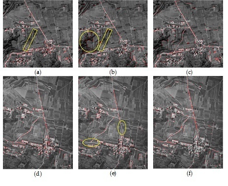
In Figure 5a–c, we can see that all three methods have completed the preliminary registration task of the No. 1 image pair, resulting in registration results that can be further optimized. However, the preregistration quality of the three methods was different. We selected two image blocks in each of the three pre-registered images with a red rectangle and a white rectangle, as shown in Figure 5a–c. The contents in the red rectangle and white rectangle both show that the method using an ANDD-based ESM gave the best registration results, followed by the method using the phase convergence model, and the worst was the method using the Canny algorithm. Table 2 also shows the method using an ANDD-based ESM resulted in the smallest RMSE and the largest D value, while the method using the Canny algorithm resulted in the largest RMSE and the smallest D value.
Figure 5d–f shows the preregistration results of No. 4 image pairs. For the two images, methods using the Canny algorithm and ANDD-based ESM registered the two images well. However, the method using the phase convergence model performed much worse as shown in Figure 5e. The RMSE of Figure 5e reached ~50 pixels, which brings difficulties for further registration processing. Although the accuracy of the pre-registration results does not directly determine the final registration accuracy, poor registration results increase the amount of computation for subsequent processing, and poorer pre-registration results may even make further processing impossible. In addition, the phase convergence model uses many parameters that need to be manually adjusted when extracting feature points, including number of wavelet scales, number of filter orientations, wave lengths of the smallest filter, scaling factors between filters, and standard deviations of log-Gabor filters. However, the method using the ANDD-based ESM only uses the standard deviation and scale factor to construct an anisotropic Gaussian kernel, which greatly reduces the number of input parameters. Based on the above experimental results and analysis, we recommend the method using the ANDD-based ESM for extracting feature points.
4.3. Effectiveness of Mutual Information
In this study, Gaussian weighted distance D and mutual information I were used as similarity metrics for registration. The authors of [8] also proposed a new metric named SMI combining spatial information and mutual information for registration, which can be simply defined as the product of D and I. However, only a pair of optical images with similar spectral responses were used to validate the metric, and some drawbacks of SMI did not show up. We tested the three metrics using two image pairs with greater differences in geometry and radiation characteristics as used in Section 4.2, and analyzed the strengths and drawbacks of these methods. The two image pairs were manually registered using ERDAS AutoSync and then a translation transformation was applied on the manually registered images. The manually registered images are shown in Figure 6. The size of the registered image of the No. 1 image pair is 762 × 397 pixels and 501 × 582 for the No. 4 image pair.
A horizontal translation with a range larger than the horizontal dimension of the reference image was implemented to demonstrate the change of D, I, and SMI. For the quantitative evaluation of D and SMI, features points should be extracted first. As analyzed in Section 4.2, we used feature points extracted with the ANDD-based ESM for all images. The distance D for the feature points under different horizontal translations with the range of [−800 800] was calculated using Equation (7) at one-pixel intervals, and the results are shown in Figure 7a. As is shown in the figure, the optimal transformation was corresponding to the global maximum of D, which helps the registration parameter converge to the optimal values. However, the global maximum of D cannot provide sub-pixel accuracy. In Figure 7d, the portion of the translation pixel with the range from −10 to 10 pixels in Figure 7a was intercepted and enlarged, and the D value was calculated at intervals of 0.1 pixels. When checked in detail as shown in Figure 7d, the maximal value of D did not correspond to the best transform parameters. This problem was caused by the outliers and mismatching of extracted features. It is common since most of the feature extraction methods do not always perform well for multi-sensor images, including the three methods used in Section 4.2.
The same transformation was applied to the No. 1 registered images to calculate the value of I. As shown in Figure 7b,e, the peak value of I was achieved when the two images were geometrically aligned. Meanwhile, Figure 7b shows that the correct transformation was at a local maximum within the range between −400 and 400 rather than the global maximum. Considering that the horizontal dimension of the reference image was 762 pixels, the mutual information-based registration method cannot support unconstrained search space. In other words, if the initial registration parameter range exceeds [−400 400], there is no guarantee that the registration result obtained is correct. This is also one reason why this method first uses the feature-based registration method to narrow the search space.
The value of SMI was further calculated using the value of D and I. The corresponding experimental results are shown in Figure 7c,f. Figure 7c shows that the global maximum of SMI was corresponding to the best transformation. Moreover, Figure 7f shows that SMI achieves the maximum value with sub-pixel registration accuracy. Therefore, in this case, SMI inherits the advantages of both D and I, and sub-pixel registration accuracy can be obtained only using the SMI metric.
In Figure 8a–c, we show the values of D, I, and SMI of the No. 4 registered images as the horizontal displacement changes from −600 pixels to 600 pixels at pixel intervals. A detail of values near the peak position is also displayed in Figure 8d–f, with the horizontal displacement changes from −10 pixels to 10 pixels at 0.1 pixel intervals. It can be seen that in this case, the D value performed similar to that as in Figure 7a. The optimal transformation was corresponding to the global maximum of D, but the registration accuracy could not achieve sub-pixel accuracy. The I value in Figure 8b performed differently compared with Figure 7b. In Figure 8b, the correct transformation corresponds to the global maximum in the entire search space. Figure 8e also shows that I achieved the maximum value with sub-pixel registration accuracy. Therefore, can be directly applied to I for the search of optimal transformation parameters when not considering computational efficiency. The SMI value in Figure 8c also shows that the global maximum of SMI was corresponding to the best transformation. However, we can see that in Figure 8f, the global maximum of SMI did not correspond to the zero position of translation. In this case, SMI inherits the advantages of D, but not I, and sub-pixel registration accuracy cannot be obtained only using the SMI metric. This phenomenon was also caused by the outliers and mismatching when extracting feature points.
The above two examples illustrate that: (1) The metric D allows the use of an unconstrained initial range, but the final registration error may be large; (2) The metric I can provide a sub-pixel registration accuracy but can only converge to the best transformation in a small search space. Therefore, preregistration using metric D should be applied to narrow the search space in advance. (3) SMI is not always able to provide sub-pixel level accuracy, and the final registration accuracy is related to the quality of the extracted feature points. Therefore, metric I performs best when a high registration accuracy is required. Meanwhile, as can be seen in Figure 7d–f and Figure 8d–f, when non-integer translation was performed, plenty of local maxima also state the difficulty of optimization. This difficulty emphasized the need to introduce as a global optimizer for all the three metrics.
4.4. Validation of the Proposed Registration Method
The reliability and validity of the proposed method were tested with various remote sensing images of different resolution ratios as described in Section 4.1. To illustrate the difference in precision between the three phases of the algorithm, the intermediate registration results are also shown. Furthermore, we have improved the SMI-based algorithm that was originally limited to rigid transformations between images of the same resolution, making it suitable for the images in this paper. In other words, the difference between the improved SMI-based method and the method in this paper was that in the improved SMI-based method, Phase-2 and Phase-3 use the SMI metric, while the NMI metric was used in the proposed method in the two phases. Then, the results of the improved SMI-based algorithm were shown to compare with the ones of the proposed method. These experiments were conducted on a computer with an Intel Core 3.50-GHz processor and 32.0 GB of physical memory.
For all image pairs, registrations were conducted with no restrictions on initial parameters. In other words, as long as there was overlap between the two images, the parameters were within the consideration of the algorithm. The parameters used for optimization and switch between the three phases were the same. For , the solution archive size was set as 50, the number of ants was set as 30, convergence speed was set as 1.35, locality of the search process was set as 0.19. Thresholds , , , and were set as 0.1. Therefore, when the diversities of parameters , , , and were smaller than 0.1, Phase-1 was terminated and Phase-2 started.
Thresholds , , , , , and for Phase-2 were set as 0.01. The number of iterations for Phase-3 was set as 200. The results of the applications of different registration methods to the five previously described pairs of images are presented in Table 3. In Table 3, the “ERDAS AutoSync” method shows registration results using CPs obtained by the APM function in ERDAS AutoSync. The transformation parameters were calculated using least square methods. The “EPFP” method shows registration results using the edge point features-based preregistration method. The “EPFP+NMI” method shows registration results using the edge point features-based preregistration method and the normalized mutual information-based registration method. Transformation parameters for the EPFP and EPFP+NMI methods were calculated for the resampled sensed image and the reference image. Therefore, these parameters were transformed based on the resample ratio to obtain transformation parameters between the original sensed image and the reference image. Then, RMSE and I values were calculated based on these parameters. The “ISMI” method shows registration results using the improved SMI-based method. The “Proposed” method shows registration results using the proposed method. As mentioned in Section 4.1, not enough CPs were extracted from the No. 5 image pair, so the ERDAS AutoSync method was not available, and the RMSE cannot be calculated for the other four methods and only I values are shown. For the No. 1 image pair, the resolution ratio was 1:1, so the three-phase method was simplified to two phases. Therefore, the results for EPFP and EPFP+NMI methods were the same. In Figure 9, the registration results using the proposed method are shown.
From Table 3, it can be observed that the proposed method generally outperformed other registration methods for all image pairs. The proposed method achieved minimum RMSE values and sub-pixel accuracy for the first four image pairs. Meanwhile, the I values reached the maximum for all five image pairs. Visual inspection of Figure 9 also verifies the registration results were accurate. It can also be seen from Table 3 that the registration accuracy of the EPFP method was the worst, and the RMSE was above 1 pixel. When the EPFP and NMI methods were used together, the RMSE value generally could be reduced to about 1 pixel. However, the resampled low-resolution sensed image lost some of the original image’s intensity information. Therefore, the registration accuracy was lower than the proposed method, which utilized the intensity information of every pixel of the original sensed image. As mentioned previously, the ISMI method combines spatial information and mutual information. Therefore, the registration accuracy using the ISMI method was related to the accuracy of the EPFP method. When the registration accuracy of the EPFP method was high, the registration accuracy of the ISMI method could be as high as the proposed method. No. 1 and No. 2 image pairs gave such examples. The RMSE of the EPFP method for the two image pairs was 2.9298 and 3.5642 pixels, which were relatively small compared with the other two image pairs. As shown in Table 3, in these cases, RMSE and I values of the ISMI and Proposed method for this image pair were almost the same. In contrast, for the No. 3 and No. 4 image pairs, the EPFP registration accuracies were relatively low. Therefore, the accuracy of the ISMI method was also lower than the proposed method.
5. Discussion
Using the method proposed to complete the registration task required three registration operations. Although the registration task in the first stage was coarse registration, it reduced the parameter search space for subsequent registration, which was very important for the convergence speed of the entire registration process. The spatial distribution of edge point features extracted from the images had an influence on registration results. To make a fair comparison, we extracted almost equal numbers of edge point features from each set of image pairs to be registered, as shown in Table 2. The spatial distribution of edge point features is shown in Figure 10. For the No. 1 image pair, the edge features were mainly boundary lines of the rivers. For the edge point features extracted from Figure 10a,d, we can see that the method using the Canny algorithm extracted just a small number of edge point features in the river boundary line at the right side of the images, especially Figure 10a. Most of the edge point features were distributed irregularly at the land area in the middle of the images. Irregular distribution of edge point features and insufficient edge point features on the strong edge (river boundary line) led to poor registration accuracy in Table 2. The edge point features extracted using the phase convergence model in Figure 10b,e had a better distribution than Figure 10a,d. In Figure 10b, moderately distributed edge point features were extracted from the river boundary line at the right side of the image. Figure 10e shows many edge point features were extracted from the water body with a short distance along the river boundary lines. This reflects that the phase convergence model was sensitive to noise when extracting edge features, which led to negative effects on registration accuracy. In Figure 10c,f, we can see that the distribution of edge point features extracted using the ANDD-based ESM from the river boundary lines in the two images were more consistent with each other. More quantity of edge point features were extracted from the river boundary line at the right side of the images in Figure 10c,f compared with Figure 10a,d, while no edge point features were extracted from the water body compared with Figure 10b,e. Therefore, Table 2 shows that the method using the ANDD-based ESM achieved the best registration results compared with the other methods.
Figure 11 shows the distribution of edge point features extracted from the No. 4 image pair with different methods. For the image pair, the edge features were mainly roads. As with Figure 10c,f, the distribution of edge point features extracted using the ANDD-based ESM of Figure 11c,f were also more consistent with each other compared with Figure 11a–d. From Figure 11a, we can see that the method using the Canny algorithm extracted just a small number of edge point features in the road inside the yellow box, which was consistent with the insufficient edge point features extracted in the river boundary line of Figure 10a. However, in other areas, both Figure 11a,d extracted edge point features that were nearly identical in distribution. As a result, the registration accuracy of the method using the Canny algorithm was a little worse than that using the ANDD-based ESM. The method using the phase convergence model performed much worse than the method using the Canny algorithm for the image pair. In Figure 11b, almost no edge points were extracted from the road in the yellow box. Figure 11e shows the method using the phase convergence model extracted some edge point features in the same road in the yellow box in Figure 11b. However, it performed not so well in other roads. For example, the method failed to extract edge point features in the roads in the yellow ellipses in Figure 11e. Besides, many point features that were not real edge points were extracted as shown in the yellow circle in Figure 11b. All the factors mentioned above led to serious inconsistency between the distributions of edge point features in Figure 11b,e. As a result, the method using the phase convergence model gave a low-level performance in Table 2 for the No. 4 image pair.
In the above analysis, the influences of different methods on the preregistration stage were discussed. Considering the entire registration strategy, we can also summarize the factors that had an impact on the registration results. Firstly, when the sensor that acquires the images to be registered has a large difference, the precision of the proposed method may be affected. For the five image pairs, only the two images of the No. 1 image pair were obtained from the optical sensor and the SAR sensor, respectively, while other images were obtained from optical sensors. We can see that the SAR image in Figure 4b is very noisy, which was also the reason why many edge point features were extracted using the phase convergence model in the water body in Figure 10e. Although the method using the ANDD-based ESM which successfully filtered the noise was adopted in the proposed method, the registration accuracy was not high in the five image pairs in Table 3. For a higher registration accuracy of such images, other similarity metrics may be considered in future studies. Secondly, resolution differences also have an impact on the registration results. For the No. 2 to No. 4 image pairs, the registration accuracy decreased as the resolution difference increased in Table 3. The reason for this phenomenon may come from increasingly significant internal distortions in high-resolution images. The high-resolution image has a larger size when the resolution difference increases. For example, the size of the high-resolution image for the No. 4 image pair was 7760 × 10,328. The distortion inside the image becomes complicated with the increase of the image. The affine transformation model for the proposed method may not accurately describe the transformation relationship between the low-resolution image and the high-resolution image. Thirdly, the land cover characteristics may have effect on the registration accuracy. The coarse registration in the proposed method was based on the edge point features. Therefore, rich edge features are necessary for image registration implementation. When the image lacks edge features, or the edge features are short and the distribution is scattered, the method is less adaptable. Temporal changes did not have an obvious impact on the registration results. As Table 1 and Table 3 show, there was no direct relationship between temporal changes and registration accuracy. However, temporal changes may bring about climate change or changes in terrain and ground facilities like buildings and roads. This makes the two images in different periods change in brightness, content, etc., thus affecting the final registration accuracy.
6. Conclusions
Many automatic registration methods have been proposed for multi-sensor remote sensing images in recent years. However, registration between images with large resolution differences has not been fully considered. As more and more sensors of different resolutions are operating in orbit, the registration of large differential resolution images will become more and more important. In this study, a new method was proposed to register images with a wide resolution ratio range from 1:1 to 50:1. Due to the difficulty and inefficiency for directly registering images with large differences in resolution, the proposed method was comprised of three phases. First, the feature-based registration method was used to provide a narrow parameter range on the reference image and the resampled sensed image for further processing. The ANDD-based ESM was used here to get more stable edge point features for registration. Then, normalized mutual information-based registration was applied on the reference image and the resampled sensed image to get more accurate transformation parameters. In the last phase, normalized mutual information-based registration was applied again on the original images to be registered.
Several image pairs with different resolution ratios were used to test the validity and practicality of the proposed method. The feature-based preregistration results showed that the ANDD-base ESM provided more stable edge point features than widely used methods, including the Canny edge detection algorithm and the phase convergence model. Registration results showed that the proposed method achieves sub-pixel accuracy and performs better than manual registration results or methods using SMI metrics in terms of matching performance and the RMSE of registration.
The larger the image data, the longer the calculation time of MI. Therefore, Phase-3 spent a lot of time when the size of the sensed image was large. Improving the speed of the proposed method is the direction of our future work.
Author Contributions
K.L. conceived and designed the experiments, developed the program, and wrote the paper. Y.Z. analyzed the results and revised the manuscript. Z.Z. and G.L. conceived of the paper and revised the manuscript.
Acknowledgments
This work was funded by the National Natural Science Foundation of China (Grant No. 41671409, 41501482), which is gratefully acknowledged.
Conflicts of Interest
The authors declare no conflicts of interest.
References
- Feyisa, G.L.; Meilby, H.; Fensholt, R.; Proud, S.R. Automated Water Extraction Index: A new technique for surface water mapping using Landsat imagery. Remote Sens. Environ. 2014, 140, 23–25. [Google Scholar] [CrossRef]
- Sotiras, A.; Davatzikos, C.; Paragios, N. Deformable medical image registration: A survey. IEEE Trans. Med. Imag. 2013, 32, 1153–1190. [Google Scholar] [CrossRef] [PubMed]
- Ma, J.; Zhao, J.; Ma, Y.; Tian, J. Non-rigid visible and infrared face registration via regularized Gaussian fields criterion. Pattern Recognit. 2015, 48, 772–784. [Google Scholar] [CrossRef]
- Leprince, S.; Barbot, S.; Ayoub, F.; Avouac, J.P. Automatic and precise orthorectification, coregistration, and subpixel correlation of satellite images, application to ground deformation measurements. IEEE Trans. Geosci. Remote Sens. 2007, 45, 1529–1558. [Google Scholar] [CrossRef]
- Liu, Z.; An, J.; Jing, Y. A simple and robust feature point matching algorithm based on restricted spatial order constraints for aerial image registration. IEEE Trans. Geosci. Remote Sens. 2012, 50, 514–527. [Google Scholar] [CrossRef]
- Brook, A.; Ben-Dor, E. Automatic registration of airborne and spaceborne images by topology map matching with SURF processor algorithm. Remote Sens. 2011, 3, 65–82. [Google Scholar] [CrossRef]
- Xing, C.; Qiu, P. Intensity-based image registration by nonparametric local smoothing. IEEE Trans. Pattern Anal. Mach. Intell. 2011, 33, 2081–2092. [Google Scholar] [CrossRef] [PubMed]
- Liang, J.; Liu, X.; Huang, K.; Li, X.; Wang, D.; Wang, X. Automatic registration of multisensor images using an integrated spatial and mutual information (SMI) metric. IEEE Trans. Geosci. Remote Sens. 2014, 52, 603–615. [Google Scholar] [CrossRef]
- Uss, M.L.; Vozel, B.; Lukin, V.V.; Chehdi, K. Multimodal remote sensing image registration with accuracy estimation at local and global scales. IEEE Trans. Geosci. Remote Sens. 2016, 54, 6587–6605. [Google Scholar] [CrossRef]
- Yan, L.; Wang, Z.; Liu, Y.; Ye, Z. Generic and automatic markov random field-based registration for multimodal remote sensing image using grayscale and gradient information. Remote Sens. 2018, 10, 1228. [Google Scholar] [CrossRef]
- Zitova, B.; Flusser, J. Image registration methods: A survey. Image Vis. Comput. 2003, 21, 977–1000. [Google Scholar] [CrossRef]
- Wong, A.; Clausi, D.A. ARRSI: Automatic registration of remote-sensing images. IEEE Trans. Geosci. Remote Sens. 2007, 45, 1483–1493. [Google Scholar] [CrossRef]
- Al-Ruzouq, R.I.; Al-Zoubi, A.; Akawi, E.E.; Abueladas, A.A.; Niemi, T.M. Multiple source imagery and linear features for detection of urban expansion in Aqaba City, Jordan. Int. J. Remote Sens. 2012, 33, 2563–2581. [Google Scholar] [CrossRef]
- Goncalves, H.; Corte-Real, L.; Goncalves, J.A. Automatic image registration through image segmentation and SIFT. IEEE Trans. Geosci. Remote Sens. 2011, 49, 2589–2600. [Google Scholar] [CrossRef]
- Misra, I.; Moorthi, S.M.; Dhar, D.; Ramakrishnan, R. An automatic satellite image registration technique based on Harris corner detection and Random Sample Consensus (RANSAC) outlier rejection model. In Proceedings of the 2012 1st International Conference on Recent Advances in Information Technology (RAIT), Dhanbad, India, 15–17 March 2012; pp. 68–73. [Google Scholar]
- Dai, X.; Khorram, S. A feature-based image registration algorithm using improved chain-code representation combined with invariant moments. IEEE Trans. Geosci. Remote Sens. 1999, 37, 2351–2362. [Google Scholar] [CrossRef]
- Leymarie, F.; Levine, M.D. Tracking deformable objects in the plane using an active contour model. IEEE Trans. Pattern Anal. Mach. Intell. 1993, 15, 617–634. [Google Scholar] [CrossRef]
- Pal, N.R.; Pal, S.K. A review on image segmentation techniques. Pattern Recognit. 1993, 26, 1277–1294. [Google Scholar] [CrossRef]
- Comaniciu, D.; Meer, P. Mean shift: A robust approach toward feature space analysis. IEEE Trans. Pattern Anal. Mach. Intell. 2002, 24, 603–619. [Google Scholar] [CrossRef]
- Cole-Rhodes, A.A.; Johnson, K.L.; LeMoigne, J.; Zavorin, I. Multiresolution registration of remote sensing imagery by optimization of mutual information using a stochastic gradient. IEEE Trans. Image Process. 2003, 12, 1495–1511. [Google Scholar] [CrossRef] [PubMed] [Green Version]
- Barbieux, K. Pushbroom hyperspectral data orientation by combining feature-based and area-based co-registration techniques. Remote Sens. 2018, 10, 645. [Google Scholar] [CrossRef]
- Tong, X.; Ye, Z.; Xu, Y.; Liu, S.; Li, L.; Xie, H.; Li, T. A novel subpixel phase correlation method using singular value decomposition and unified random sample consensus. IEEE Trans. Geosci. Remote Sens. 2015, 53, 4143–4156. [Google Scholar] [CrossRef]
- Gong, M.; Zhao, S.; Jiao, L.; Tian, D.; Wang, S. A novel coarse-to-fine scheme for automatic image registration based on SIFT and mutual information. IEEE Trans. Geosci. Remote Sens. 2014, 52, 4328–4338. [Google Scholar] [CrossRef]
- Behan, A. 2-D and 3-D Image Registration for Medical, Remote Sensing, and Industrial Applications. Photogramm. Rec. 2006, 21, 180–181. [Google Scholar] [CrossRef]
- Holden, M. A review of geometric transformations for nonrigid body registration. IEEE Trans. Med. Imag. 2008, 27, 111–128. [Google Scholar] [CrossRef] [PubMed]
- Bowen, R.; Chazottes, J.R. Equilibrium States and the Ergodic Theory of Anosov Diffeomorphisms; Springer: Berlin/Heidelberg, Germany, 1975; p. 470. [Google Scholar]
- Le Moigne, J.; Campbell, W.J.; Cromp, R.F. An automated parallel image registration technique based on the correlation of wavelet features. IEEE Trans. Geosci. Remote Sens. 2002, 40, 1849–1864. [Google Scholar] [CrossRef] [Green Version]
- Thévenaz, P.; Unser, M. Optimization of mutual information for multiresolution image registration. IEEE Trans. Image Process. 2000, 9, 2083–2099. [Google Scholar] [CrossRef] [PubMed] [Green Version]
- Wu, Y.; Ma, W.; Miao, Q.; Wang, S. Multimodal continuous ant colony optimization for multisensor remote sensing image registration with local search. Swarm Evol. Comput. 2017, 7, 1–10. [Google Scholar] [CrossRef]
- Dorigo, M.; Maniezzo, V.; Colorni, A. Ant system: Optimization by a colony of cooperating agents. IEEE Trans. Syst. Man Cybern. B Cybern. 1996, 26, 29–41. [Google Scholar] [CrossRef] [PubMed]
- Socha, K.; Dorigo, M. Ant colony optimization for continuous domains. Eur. J. Oper. Res. 2008, 185, 1155–1173. [Google Scholar] [CrossRef] [Green Version]
- Yang, Q.; Chen, W.N.; Yu, Z.; Gu, T.; Li, Y.; Zhang, H.; Zhang, J. Adaptive multimodal continuous ant colony optimization. IEEE Trans. Evol. Comput. 2017, 21, 191–205. [Google Scholar] [CrossRef]
- Jiang, Y.H.; Zhang, G.; Tang, X.M.; Li, D.; Huang, W.C.; Zhang, H.; Pan, H.B. Geometric calibration and accuracy assessment of ZiYuan-3 multispectral images. IEEE Trans. Geosci. Remote Sens. 2014, 52, 4161–4172. [Google Scholar] [CrossRef]
- Zhang, G.; Jiang, Y.; Li, D.; Li, D.; Huang, W.; Pan, H.B.; Tang, X.; Zhu, X. In-orbit geometric calibration and validation of ZY-3 linear array sensors. Photogramm. Rec. 2014, 29, 68–88. [Google Scholar] [CrossRef]
- Zhang, Y.; Zheng, M.; Xiong, J.; Lu, Y.; Xiong, X. On-orbit geometric calibration of ZY-3 three-line array imagery with multistrip data sets. IEEE Trans. Geosci. Remote Sens. 2014, 52, 224–234. [Google Scholar] [CrossRef]
- Yang, B.; Wang, M.; Xu, W.; Li, D.; Gong, J.; Pi, Y. Large-scale block adjustment without use of ground control points based on the compensation of geometric calibration for ZY-3 images. ISPRS-J. Photogramm. Remote Sens. 2017, 134, 1–14. [Google Scholar] [CrossRef]
- Zambanini, S.; Sablatnig, R. A Hough Voting Strategy for Registering Historical Aerial Images to Present-Day Satellite Imagery. In Proceedings of the International Conference on Image Analysis and Processing, Catania, Italy, 11–15 September 2017; pp. 595–605. [Google Scholar]
- Canny, J. A computational approach to edge detection. IEEE Trans. Pattern Anal. Mach. Intell. 1986, 8, 679–698. [Google Scholar] [CrossRef] [PubMed]
- Smith, T.G., Jr.; Marks, W.B.; Lange, G.D.; Sheriff, W.H.; Neale, E.A. Edge detection in images using Marr-Hildreth filtering techniques. J. Neurosci. Meth. 1988, 26, 75–81. [Google Scholar] [CrossRef]
- Shui, P.L.; Zhang, W.C. Noise-robust edge detector combining isotropic and anisotropic Gaussian kernels. Pattern Recognit. 2012, 45, 806–820. [Google Scholar] [CrossRef]
- Zhang, W.C.; Shui, P.L. Contour-based corner detection via angle difference of principal directions of anisotropic Gaussian directional derivatives. Pattern Recognit. 2015, 48, 2785–2797. [Google Scholar] [CrossRef]
- Alhichri, H.S.; Kamel, M. Multi-resolution image registration using multi-class Hausdorff fraction. Pattern Recognit. Lett. 2002, 23, 279–286. [Google Scholar] [CrossRef]
- Peng, X.; Chen, W.; Ma, Q. Feature-based nonrigid image registration using a Hausdorff distance matching measure. Opt. Eng. 2007, 46, 057201. [Google Scholar] [CrossRef]
- Maes, F.; Collignon, A.; Vandermeulen, D.; Marchal, G.; Suetens, P. Multimodality image registration by maximization of mutual information. IEEE Trans. Med. Image. 1997, 3, 154–196. [Google Scholar] [CrossRef] [PubMed]
- Ma, J.; Zhou, H.; Zhao, J.; Gao, Y.; Jiang, J.; Tian, J. Robust feature matching for remote sensing image registration via locally linear transforming. IEEE Trans. Geosci. Remote Sens. 2015, 53, 6469–6481. [Google Scholar] [CrossRef]
- Kern, J.P.; Pattichis, M.S. Robust multispectral image registration using mutual-information models. IEEE Trans. Geosci. Remote Sens. 2007, 45, 1494–1505. [Google Scholar] [CrossRef]
- IMAGINE AutoSync™ User’s Guide. Available online: http://faculty.une.edu/cas/szeeman/rs/docs/AutoSync.pdf (accessed on 14 February 2019).
Figure 1.
Flowchart of the proposed method. ACO: ant colony optimization.

Figure 2.
Illustration of the edge strength maps (ESMs) of a noisy image: (a) a noisy synthetic cartoon image with noise; (b) small-scaled gradient-based ESM; (c) ANDD-based ESM with the same edge resolution; (d) fused ESM.
Figure 2.
Illustration of the edge strength maps (ESMs) of a noisy image: (a) a noisy synthetic cartoon image with noise; (b) small-scaled gradient-based ESM; (c) ANDD-based ESM with the same edge resolution; (d) fused ESM.

Figure 3.
Simple examples of measurement D. (a) The distances between the dots and the nearest triangle (connected with a dotted line) are 1. (b) The distances between the dots and the nearest triangle are 1 with an outlier in the lower right corner with a distance of 10.
Figure 3.
Simple examples of measurement D. (a) The distances between the dots and the nearest triangle (connected with a dotted line) are 1. (b) The distances between the dots and the nearest triangle are 1 with an outlier in the lower right corner with a distance of 10.

Figure 4.
Image pairs to be registered. The specific parameters of Figure 4a–j are listed in Table 1. Red points in the images show the spatial distribution of extracted control points (CPs) using Automatic Point Measurement (APM).


Figure 5.
Feature-based preregistration results using different edge points extraction methods. (a,d) use the Canny algorithm to obtain edge points; (b,e) use the phase convergence model to obtain edge points; (c,f) use the ANDD-based ESM to obtain edge points.
Figure 5.
Feature-based preregistration results using different edge points extraction methods. (a,d) use the Canny algorithm to obtain edge points; (b,e) use the phase convergence model to obtain edge points; (c,f) use the ANDD-based ESM to obtain edge points.

Figure 6.
Manually registered images using ERDAS AutoSync. (a) The green component and red component are the reference image and the warped sensed image of the No. 1 image pairs, respectively; (b) the green component and red component are the reference image and the warped sensed image of the No. 4 image pairs, respectively.

Figure 7.
D, I, and SMI values under different horizontal translations between the manually registered images in Figure 6a. (a–c) are the D, I, and SMI values when the horizontal displacement is between [−800 800] at pixel intervals; (d–f) are the D, I, and SMI values when the horizontal displacement is between [−10 10] at 0.1 pixel intervals.

Figure 8.
D, I, and SMI values under different horizontal translations between the manually registered images in Figure 6b. (a–c) are the D, I, and SMI values when the horizontal displacement is between [−600 600] at pixel intervals; (d–f) are the D, I, and SMI values when the horizontal displacement is between [−10 10] at 0.1 pixel intervals.

Figure 9.
Registration results using the proposed method displayed as a checkerboard mosaicked image. (a–e) are registered images for No. 1–5 image pairs.
Figure 9.
Registration results using the proposed method displayed as a checkerboard mosaicked image. (a–e) are registered images for No. 1–5 image pairs.

Figure 10.
Feature-based preregistration results using different edge points extraction methods for the No. 1 image pair. (a,d) use the Canny algorithm to obtain edge points; (b,e) use the phase convergence model to obtain edge points; (c,f) use the ANDD-based ESM to obtain edge points.
Figure 10.
Feature-based preregistration results using different edge points extraction methods for the No. 1 image pair. (a,d) use the Canny algorithm to obtain edge points; (b,e) use the phase convergence model to obtain edge points; (c,f) use the ANDD-based ESM to obtain edge points.

Figure 11.
Feature-based preregistration results using different edge points extraction methods for the No. 4 image pair. (a,d) use the Canny algorithm to obtain edge points; (b,e) use the phase convergence model to obtain edge points; (c,f) use the ANDD-based ESM to obtain edge points.
Figure 11.
Feature-based preregistration results using different edge points extraction methods for the No. 4 image pair. (a,d) use the Canny algorithm to obtain edge points; (b,e) use the phase convergence model to obtain edge points; (c,f) use the ANDD-based ESM to obtain edge points.


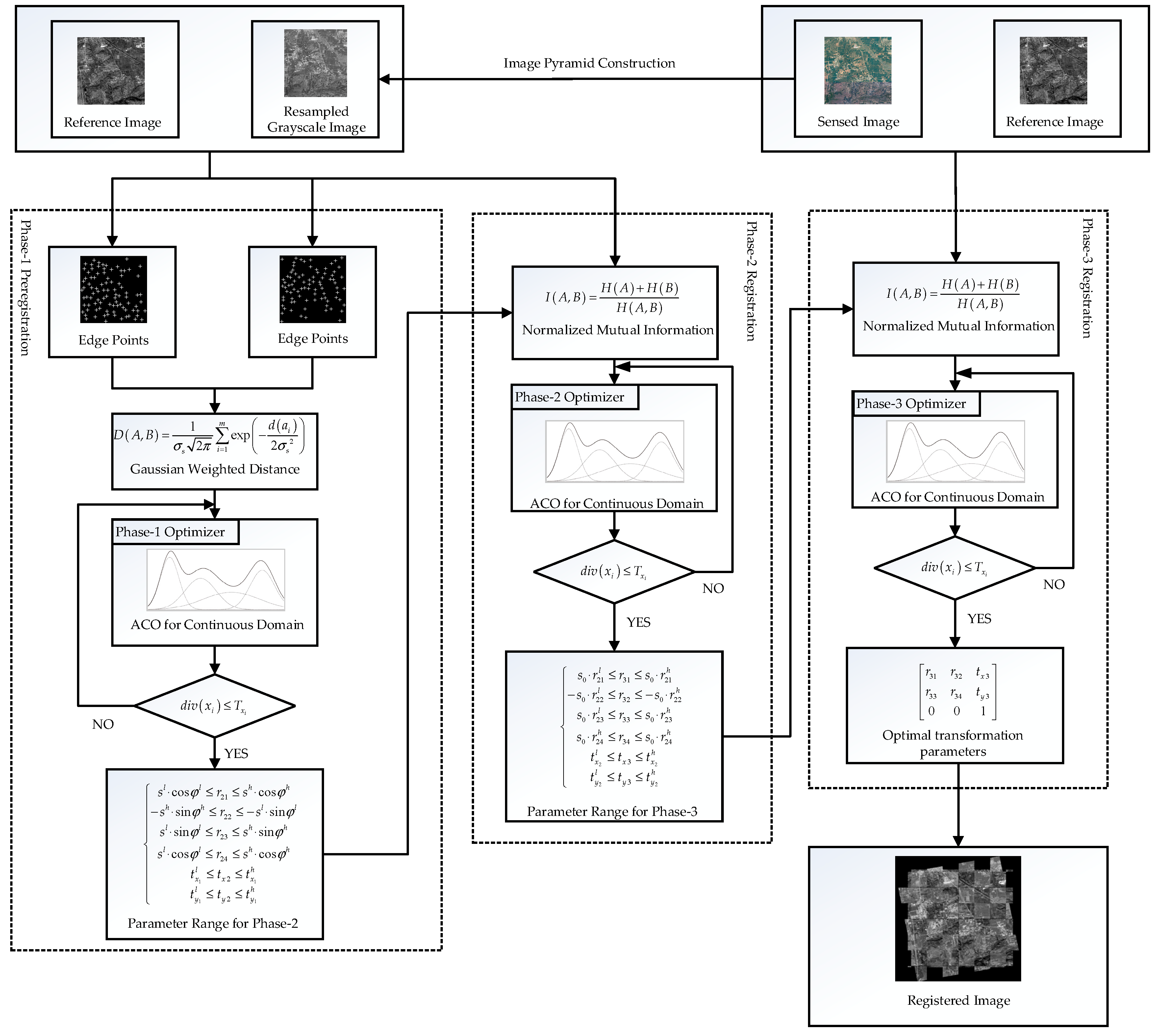
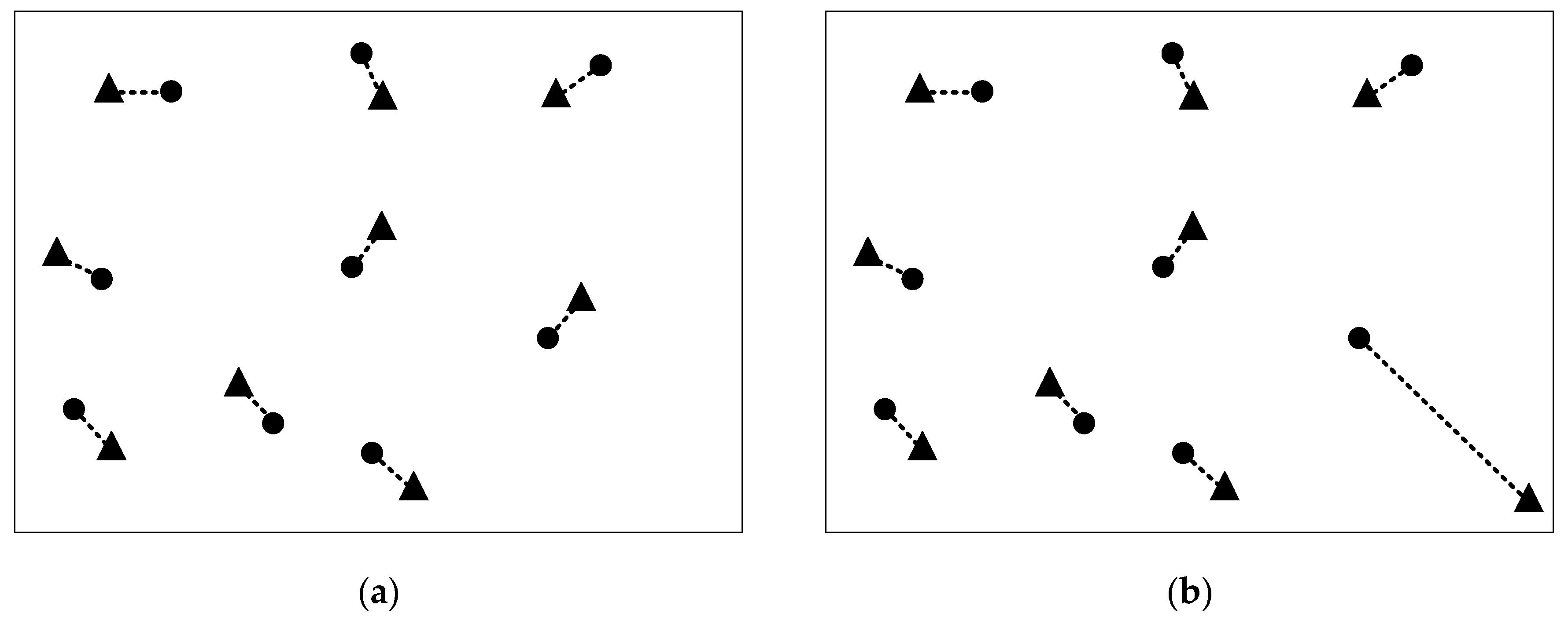
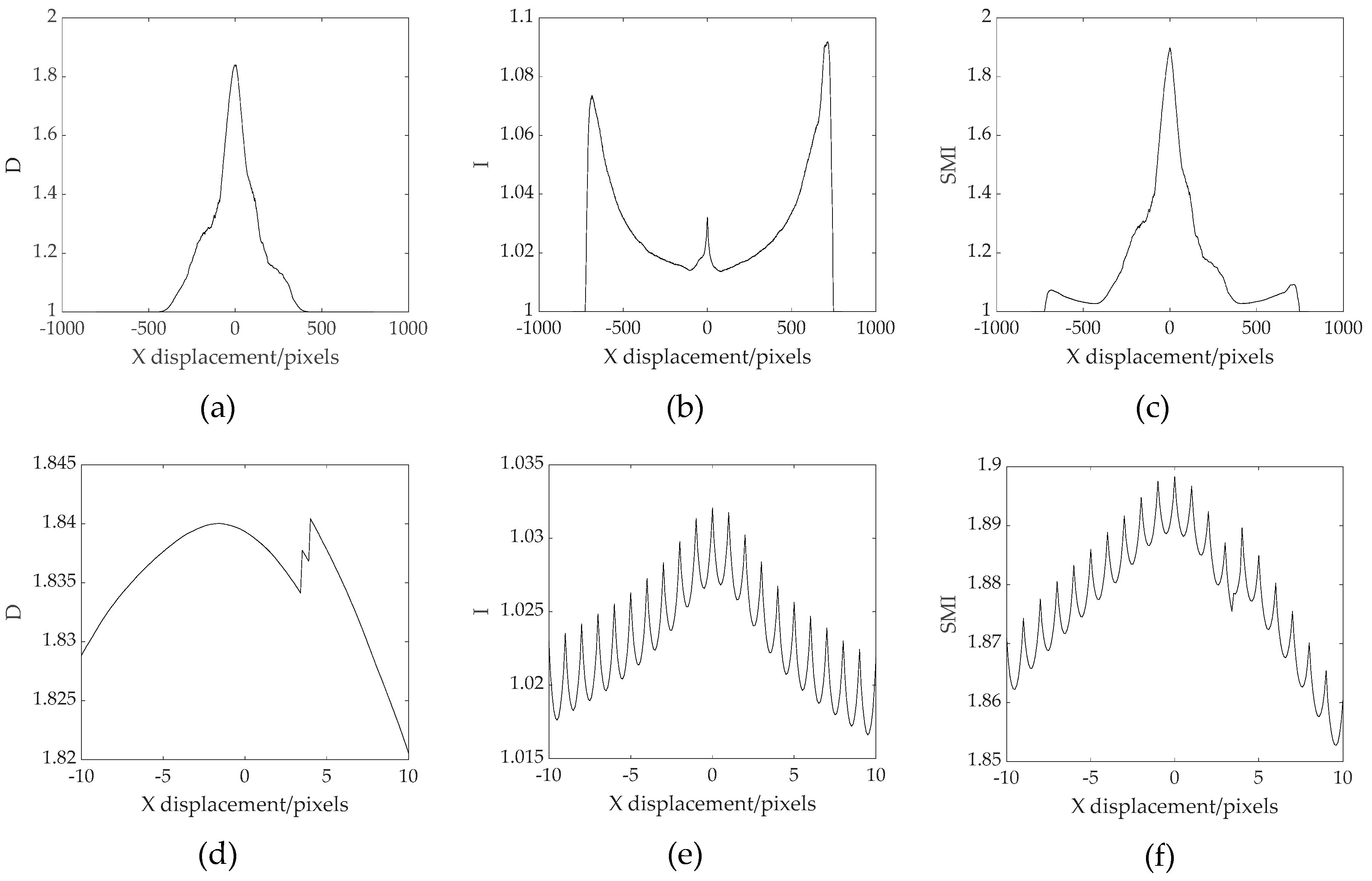
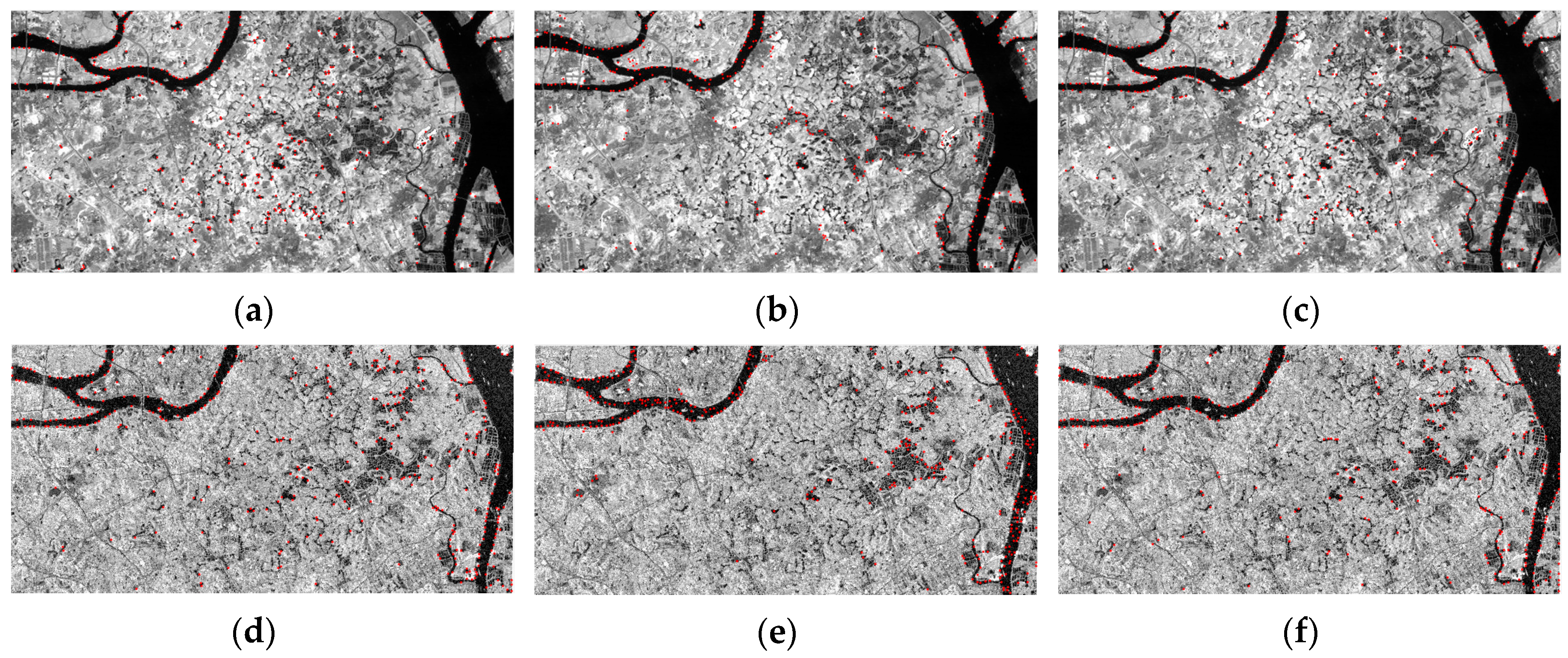
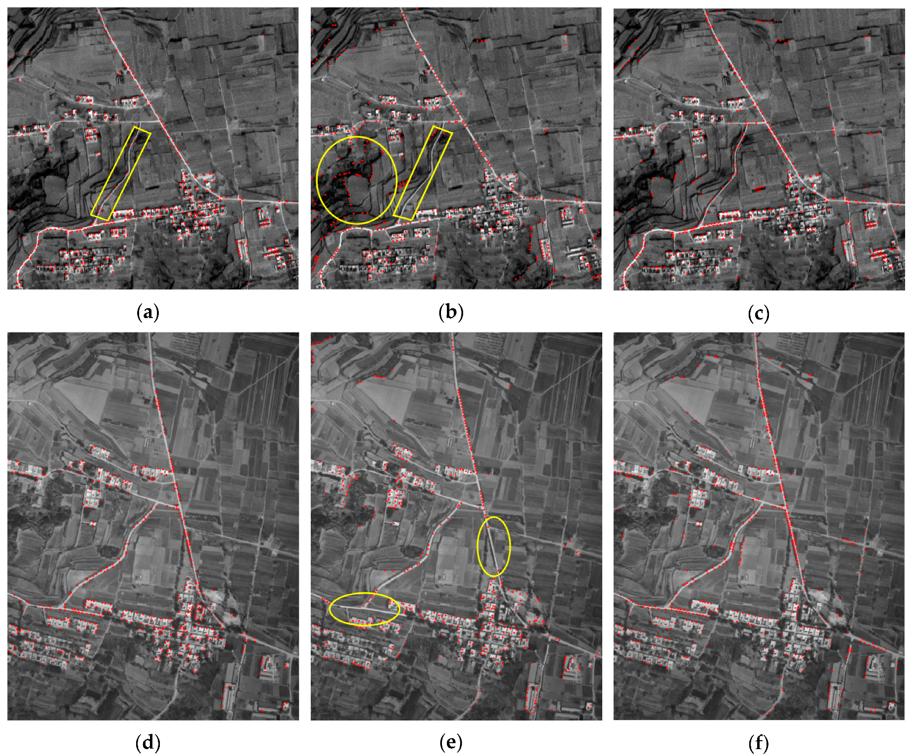
Table 1.
Specific parameters of image pairs to be registered. GSD: ground sampling distance; SAR: synthetic aperture radar.
Table 1.
Specific parameters of image pairs to be registered. GSD: ground sampling distance; SAR: synthetic aperture radar.
| No. | Figure | Data Source | Image Size (pixels) | GSD (m) | Resolution Ratio | Date | Location |
|---|---|---|---|---|---|---|---|
| 1 | 4a | Landsat TM | 762 × 379 | 30 | 1:1 | 2007 | China, Guangzhou |
| 4b | SAR | 696 × 344 | 30 | 2008 | |||
| 2 | 4c | Ziyuan-3 | 162 × 165 | 2.1 | 4:1 | 2013 | China, Dengfeng |
| 4d | Aerial DOM | 700 × 700 | 0.5 | 2010 | |||
| 3 | 4e | Tianhui-1 | 500 × 500 | 5 | 10:1 | 2016 | China, Dengfeng |
| 4f | Aerial DOM | 5048 × 5671 | 0.5 | 2010 | |||
| 4 | 4g | Ziyuan-3 | 463 × 449 | 2.1 | 21:1 | 2013 | China, Dengfeng |
| 4h | Phase One | 7760 × 10,328 | 0.1 | 2015 | |||
| 5 | 4i | Tianhui-1 | 172 × 191 | 5 | 50:1 | 2016 | China, Dengfeng |
| 4j | Phase One | 7760 × 10,328 | 0.1 | 2015 |
Table 2.
Experimental results of features-based preregistration. RMSE: root mean square error; D: Gaussian weighted distance-based similarity metric.
Table 2.
Experimental results of features-based preregistration. RMSE: root mean square error; D: Gaussian weighted distance-based similarity metric.
| No. | Method | Edge Points No. | RMSE (pixels) | D |
|---|---|---|---|---|
| 1 | Canny | 395/384 | 7.56 | 1.85 |
| phase | 395/398 | 5.18 | 1.86 | |
| Proposed | 393/384 | 2.93 | 1.88 | |
| 4 | Canny | 406/415 | 11.51 | 1.89 |
| phase | 401/412 | 50.22 | 1.86 | |
| Proposed | 409/420 | 10.76 | 1.90 |
Table 3.
Experimental results of different registration methods. EPFP: edge point features-based preregistration method; NMI: normalized mutual information-based registration method; ISMI: improved SMI-based method.
Table 3.
Experimental results of different registration methods. EPFP: edge point features-based preregistration method; NMI: normalized mutual information-based registration method; ISMI: improved SMI-based method.
| No. | Methods | RMSE (pixels) | I | ||||||
|---|---|---|---|---|---|---|---|---|---|
| 1 | ERDAS AutoSync | 0.9964 | −0.0449 | 0.0533 | 0.9964 | 30.9492 | 5.8776 | 0.9339 | 1.0334 |
| EPFP | 1.0029 | −0.0413 | 0.0413 | 1.0029 | 28.4385 | 7.6797 | 2.9298 | 1.0292 | |
| EPFP +NMI | 0.9941 | −0.0472 | 0.0532 | 0.9972 | 31.9530 | 5.8181 | 0.8658 | 1.0337 | |
| ISMI | 0.9983 | −0.0462 | 0.0526 | 0.9969 | 30.1811 | 6.1581 | 0.8730 | 1.0334 | |
| Proposed | 0.9941 | −0.0472 | 0.0532 | 0.9972 | 31.9530 | 5.8181 | 0.8658 | 1.0337 | |
| 2 | ERDAS AutoSync | 0.2384 | 0.0443 | −0.0449 | 0.2390 | −14.3516 | 10.6895 | 0.6632 | 1.0466 |
| EPFP | 0.2268 | 0.0442 | −0.0442 | 0.2268 | −13.3705 | 14.6342 | 3.5642 | 1.0257 | |
| EPFP +NMI | 0.2384 | 0.0449 | −0.0463 | 0.2373 | −14.8262 | 10.8282 | 0.3858 | 1.0528 | |
| ISMI | 0.2380 | 0.0450 | −0.0465 | 0.2375 | −14.6429 | 10.9147 | 0.3608 | 1.0544 | |
| Proposed | 0.2379 | 0.0454 | −0.0465 | 0.2374 | −14.6659 | 10.9359 | 0.3447 | 1.0546 | |
| 3 | ERDAS AutoSync | 0.0981 | 0.0185 | −0.0186 | 0.0967 | −58.3673 | 25.8779 | 0.5678 | 1.0260 |
| EPFP | 0.0979 | 0.0145 | −0.0145 | 0.0979 | −46.7202 | 25.5249 | 14.8270 | 1.0052 | |
| EPFP +NMI | 0.0979 | 0.0184 | −0.0188 | 0.0968 | −57.5111 | 27.0336 | 1.2557 | 1.0195 | |
| ISMI | 0.0986 | 0.0182 | −0.0177 | 0.0962 | −58.1402 | 26.6876 | 0.7155 | 1.0250 | |
| Proposed | 0.0980 | 0.0185 | −0.0185 | 0.0967 | −58.2511 | 25.9319 | 0.5765 | 1.0261 | |
| 4 | ERDAS AutoSync | 0.0448 | 0.0148 | −0.0151 | 0.0447 | −32.4730 | 40.3796 | 1.1232 | 1.0184 |
| EPFP | 0.0464 | 0.0165 | −0.0165 | 0.0464 | −54.2718 | 32.6967 | 10.7569 | 1.0082 | |
| EPFP +NMI | 0.0449 | 0.0148 | −0.0153 | 0.0449 | −33.8550 | 39.7711 | 1.3231 | 1.0173 | |
| ISMI | 0.0450 | 0.0147 | −0.0154 | 0.0448 | −33.3337 | 40.8091 | 1.5782 | 1.0157 | |
| Proposed | 0.0448 | 0.0147 | −0.0152 | 0.0447 | −32.1441 | 40.7132 | 0.8396 | 1.0191 | |
| 5 | ERDAS AutoSync | - | - | - | - | - | - | - | - |
| EPFP | 0.0190 | 0.0054 | −0.0054 | 0.0190 | −13.6224 | 18.5911 | - | 1.0223 | |
| EPFP +NMI | 0.0186 | 0.0059 | −0.0059 | 0.0180 | −13.4551 | 22.8200 | - | 1.0268 | |
| ISMI | 0.0188 | 0.0061 | −0.0059 | 0.0183 | −14.9141 | 21.4645 | - | 1.0282 | |
| Proposed | 0.0186 | 0.0059 | −0.0059 | 0.0181 | −12.6220 | 22.3736 | - | 1.0290 |
© 2019 by the authors. Licensee MDPI, Basel, Switzerland. This article is an open access article distributed under the terms and conditions of the Creative Commons Attribution (CC BY) license (http://creativecommons.org/licenses/by/4.0/).
Share and Cite
MDPI and ACS Style
Li, K.; Zhang, Y.; Zhang, Z.; Lai, G. A Coarse-to-Fine Registration Strategy for Multi-Sensor Images with Large Resolution Differences. Remote Sens. 2019, 11, 470. https://0-doi-org.brum.beds.ac.uk/10.3390/rs11040470
AMA Style
Li K, Zhang Y, Zhang Z, Lai G. A Coarse-to-Fine Registration Strategy for Multi-Sensor Images with Large Resolution Differences. Remote Sensing. 2019; 11(4):470. https://0-doi-org.brum.beds.ac.uk/10.3390/rs11040470
Chicago/Turabian StyleLi, Kai, Yongsheng Zhang, Zhenchao Zhang, and Guangling Lai. 2019. "A Coarse-to-Fine Registration Strategy for Multi-Sensor Images with Large Resolution Differences" Remote Sensing 11, no. 4: 470. https://0-doi-org.brum.beds.ac.uk/10.3390/rs11040470
Note that from the first issue of 2016, this journal uses article numbers instead of page numbers. See further details here.