Multiple Remotely Sensed Lines of Evidence for a Depleting Seasonal Snowpack in the Near East


1
Eurasia Institute of Earth Sciences, Istanbul Technical University, Maslak 34469, Istanbul, Turkey
2
Department of Geosciences, University of Oslo, P.O. Box 1047, Blindern, 0316 Oslo, Norway
*
Author to whom correspondence should be addressed.
Remote Sens. 2019, 11(5), 483; https://0-doi-org.brum.beds.ac.uk/10.3390/rs11050483
Submission received: 18 January 2019
/
Revised: 8 February 2019
/
Accepted: 21 February 2019
/
Published: 26 February 2019
Abstract
:The snow-fed river basins of the Near East region are facing an urgent threat in the form of declining water resources. In this study, we analyzed several remote sensing products (optical, passive microwave, and gravimetric) and outputs of a meteorological reanalysis data set to understand the relationship between the terrestrial water storage anomalies and the mountain snowpack. The results from different satellite retrievals show a clear signal of a depletion of both water storage and the seasonal snowpack in four basins in the region. We find a strong reduction in terrestrial water storage over the Gravity Recovery and Climate Experiment (GRACE) observational period, particularly over the higher elevations. Snow-cover duration estimates from Moderate Resolution Imaging Spectroradiometer (MODIS) products point towards negative and significant trends up to one month per decade in the current era. These numbers are a clear indicator of the partial disappearance of the seasonal snow-cover in the region which has been projected to occur by the end of the century. The spatial patterns of changes in the snow-cover duration are positively correlated with both GRACE terrestrial water storage decline and peak snow water equivalent (SWE) depletion from the ERA5 reanalysis. Possible drivers of the snowpack depletion are a significant reduction in the snowfall ratio and an earlier snowmelt. A continued depletion of the montane snowpack in the Near East paints a bleak picture for future water availability in this water-stressed region.
Keywords:
snow cover; snow water equivalent; near east; water resources; GRACE; MODIS; AMSR-E; AMSR2; ERA5; euphrates; tigris; Kura-Araks; Coruh; Van Lake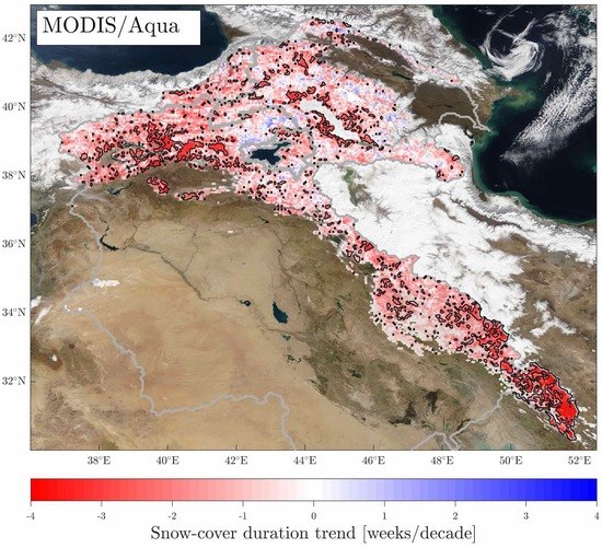
1. Introduction
The Near East region that encompasses the Fertile Crescent, often referred to as the cradle of civilization, has long been a center of agricultural activity. This has largely been due to a warm climate, nutrient-rich soil and the abundance of fresh water supplied by large snow-fed rivers such as the Tigris and the Euphrates. Presently, the waters of these rivers, being an essential resource for about 81 million people [1], are used extensively for industry, hydropower, and agriculture. Historically, prolonged droughts and a lack of water security have been major sources of conflict in this water-stressed region [2,3,4,5]. Currently, the water resources of the Near East are reported as highly vulnerable [6,7] with severe water scarcity throughout the year [8]. Worryingly, the sustainable use of this region’s water resources is threatened by the projected climate change related both to greenhouse forcing and land use change [6,9,10,11].
Several studies point out that the climate of the Near East region has been changing during recent decades (e.g., [12,13,14,15,16]). In the current era, the year 2007 was an important milestone for the region in terms of water resources. Strong observational evidence of a long-term drought in the Fertile Crescent was shown for the 2007–2009 period in the study of Trigo et al. [12]. Türkeş et al. [15] reported significant changes in the temperature pattern over the coasts of the Black Sea and the eastern Anatolia where the headwaters of the Euphrates and Tigris basin (ETB) are located. They also found that the average precipitation increased by 1.9 mm per month from 1950–1980 to 1981–2010 for these areas. In their clustering analysis, they showed the formation of a new continental rainy summer precipitation pattern over northeastern Anatolia after 1980. For the same area, Gokmen [16] found an increasing trend of total annual precipitation over the period 1979–2010 up to 150 mm that agrees with the ERA-Interim/Land reanalysis data. The analysis of Gokmen [16] also indicated a significant decreasing trend in annual precipitation over the lower elevations in the ETB from station data and two reanalysis data sets. Several studies have projected a temperature increase pattern in the future over the Near East. Both global [17,18,19] and regional [9,10,20,21,22,23] climate modeling studies projected an absolute increase in the future temperature of around 1–9 C (depending on the scenario and the model) over the region at the end of the 21st century. The direction and the magnitude of the projected changes in precipitation vary depending on the season and the subregion. Future simulations estimate a decrease in precipitation over the Near East region with an exception of winter months and the coasts of the Black Sea region [10,22,23,24]. In a statistical analysis, Ezber [25] used the outputs of future CORDEX simulations [26] to show a significant shift in precipitation seasonality over the Black Sea region and southeastern Anatolia. All these studies point towards the Near East being a region that is especially vulnerable to climate change. These findings indicate that the water resources of the region may be under threat in the future.
Temperature has a direct effect on snow processes through modulating the phase of precipitation and the persistence of the snow once it is on the ground [27]. Both ground observations [13,14] and satellite products [28] show that increasing temperatures (up to 2 C) have led to earlier spring snowmelt in the mountainous parts of the ETB. Sen et al. [13] investigated the changes in discharge timing in the ETB and teleconnection patterns, and concluded that earlier snowmelt typically occurs during the negative phase of the North Sea–Caspian pattern. The role of large-scale climate anomalies, particularly those related to La Niña, in forming droughts in the Middle East was studied by Barlow et al. [29]. They underlined the fact that projections point towards a drying and warming of the climate in the region, leading to a reduction in peak snow water equivalent (SWE) and earlier snowmelt. Yucel et al. [14] showed that streamflow timing in eastern Anatolia is already occurring over a week earlier compared to the climatological average for the period 1970–2010. By running regional climate simulations under a high emissions scenario, they projected that by the end of the century this shift would be as large as one month. The end of century projections also showed a considerable decrease in surface runoff for the Aras basin and the ETB, while a lower decline was found for the Coruh basin. In a hydrological modeling study, Bozkurt et al. [30] found similar results, projecting a decrease of 19–58% in annual streamflow in the ETB by the end of the century, corresponding to a temporal shift of streamflow timing of around 3–5 weeks. Ozdogan [31] evaluated the snow water availability in the whole ETB by forcing their model with the outputs of several regional climate simulations. Even though the results (decrease in SWE between 10 to 60%) show variations due to the different input data, they agreed on a significant decrease in SWE in the lower elevations (under 500 m) by the end of the century. A comprehensive analysis of snowmelt projections for different elevation bands was conducted by Onol et al. [10] for the ETB. Their five different regional climate model outputs projected that the seasonal snow cover would vanish in the lower regions (elevation between 1000 and 1500 m) at the end of the century. Moreover, snow in the middle and higher elevation regions (elevation > 1500 m) were projected to share the same destiny for the model outputs forced under various future scenarios. It is important to emphasize that other than reducing snowfall, drying has another important effect in that it may lead to an increase in snowpack ablation through sublimation [32]. These projections, including business as usual, paint a bleak picture for the future of the water resources of the Near East region.
Observations from space play an important role in monitoring changes in the state of the Earth’s surface [33,34,35] including the global terrestrial water storage [36] and the snowpack [37,38]. The globally available satellite retrievals of total terrestrial water storage (TWS) from the Gravity Recovery and Climate Experiment (GRACE) [39] are invaluable for diagnosing the state of water resources in areas such as the Near East where the availability of ground observations are both physically and politically limited. The GRACE TWS retrieval represents the water equivalent thickness which is the aggregate of all the water storage components within a pixel, namely soil moisture, surface water, groundwater, ice and snow (e.g., [36,40,41,42,43]). Voss et al. [40] used GRACE data to show the ongoing water loss in the Tigris-Euphrates-Western Iran region. They used the outputs of NASA’s Global Land Data Assimilation System (GLDAS) to decompose the GRACE TWS signal into its various storage components. Through this approach, they estimated a groundwater depletion of mm yr for the period between 2003 and 2009. Longuevergne et al. [41] underlined that the groundwater contribution to the GRACE observation can be underestimated by half if the spatial distribution of the reservoirs is not considered in the ETB. Another study for this region was conducted by Joodaki et al. [42] using GRACE TWS data, a land surface model, and well observations. Their model outputs showed that a decrease in groundwater storage is the reason for a negative GRACE TWS trend pattern mainly centered over the northern part of the Iraq-Iran border. After the drought in 2007, the human-induced groundwater loss was recovered in the upper part of the ETB by 2013. The same recovery was not found for the groundwater storage in Iran [42]. In another study, Forootan et al. [43] found that total water flux values derived from GRACE and those obtained from two reanalysis datasets (ERA-Interim and MERRA-Land) had high correlations for the mountainous regions of the ETB. They calculated negative water flux trends of around −2.6 mm month yr. Recently, Rodell et al. [36] estimated a decrease in total water storage of around Gt yr for the northern Middle East region which includes eastern Turkey, Iran, Iraq, and Syria. They claimed that a large negative trend occurred because of groundwater depletion and drought which are categorized as a “possible or partial direct human impact”. All these findings point towards an already severe depletion of water resources in the region.
Decomposing the total water storage into its components shows a clear signal of groundwater depletion in the Near East region [36,40,41,42,43]. Additionally, surface soil moisture trends show a significant decrease for the Middle East region [44]. Similar results were found over a longer time period by Feng and Zhang [45]. They also showed a drying tendency in the arid land areas. Among the components of TWS, the mountain snowpack, typically expressed as the volume (or mass) of SWE, is an important but less studied part of this equation in the Near East. In this region, the high mountain snowpack acts as a water tower [46]. It is thus important to better understand the role of snow in the TWS signal. For investigating the snowpack in data sparse regions such as the Near East, satellite remote sensing is an invaluable tool for monitoring the state of the snowpack (e.g., [37]). The disadvantage with satellite remote sensing of snow is that at present accurate retrieval of SWE, the main quantity of interest, is not possible over complex terrain [47,48]. Also, the most reliable retrievals, namely the optically based retrievals of snow-covered area, have trouble sensing in cloudy conditions, resulting in large data gaps (e.g., [49]). Nonetheless, SWE is strongly correlated with snow-cover duration [48] and many previous studies have successfully used optical remote sensing to study the evolution of the snow-cover (e.g., [38,50]). For the Near East, the accuracy of Moderate Resolution Imaging Spectroradiometer (MODIS) snow-cover products (MOD10A1 and MOD10A2) has been evaluated through several studies conducted in the Karasu basin located in the headwaters of the Euphrates River [51,52,53,54]. These early studies reveal that these products were reasonably accurate, although clouds were a notable source of error. Ensuing studies in the Karasu basin reduced the cloud problem by making use of the composite 8-day MODIS snow-cover product (MOD10C2) and passive microwave SWE retrievals [28,55]. It was found that a decrease in precipitation and increase in temperature had led to a decrease in peak discharge amounts and an earlier snowmelt timing in both the 2008 and 2009 water years [28]. A strong negative correlation was found between the MODIS snow-covered area and in situ runoff which is not surprising given that 60–70% of the annual streamflow in the Karasu basin is snowmelt runoff [56]. Snowmelt estimation is thus important in the context of managing the water resources of this region. For this purpose, several studies [56,57,58,59,60] developed different methods for forecasting the daily snow cover and streamflow.
Changes in peak SWE and snowmelt timing may already be playing an important role in the observed TWS signal over the GRACE observation period (2002–2017). In this study, we conduct an exploratory analysis to investigate the role of the snowpack in the observed decrease in water storage of the transboundary basins of the Near East region. We analyze several snow-related satellite retrievals (optical, passive microwave and gravimetric) and a new meteorological reanalysis data set for this semi-arid region. Both the temporal trends in the individual data sets and correlations between them are considered in the analysis.
2. Study Area
The Near East region is the land area nestled between the Mediterranean Sea, Black Sea, Caspian Sea, Arabian Sea, and Red Sea. Among the main river basins of this territory are the ETB, Kura-Araks basin (KAB), Çoruh basin (COB), and the Van Lake basin (VAN) (Figure 1). Except for the latter, these are all transboundary river basins. All these basins are snow-fed river basins which are vulnerable to projected climate change [7,10,20]. The waters of these basins are distributed to populations of around 65.5 million, 14.5 million, 790 thousand, and 950 thousand people respectively [61]. The ETB as the largest (Table 1) basin is assumed to be the most important water resource in the Middle East region [20], while KAB is the main water source of the South Caucasus region [1,62]. The Euphrates and the Tigris rivers have a length of approximately 3000 km and 1850 km, respectively. Both rise at the highlands of eastern Anatolia and flow into the Persian Gulf. The Kura River originates in Georgia, while the Araks River starts in Turkey. They are approximately 1515 km and 1072 km long, respectively, and both end in the Caspian Sea [1]. The Coruh River, with a length of 426 km, originates in northeastern Turkey, and reaches to the Black Sea [63]. In the total basin area, annual discharge amounts are about 147.67, 25.28, and 13.07 km/year for the ETB, KAB, and COB, while annual runoff is 170.12, 133.02, and 592.95 mm/year, respectively [61]. VAN is an endorheic, i.e., hydrologically closed, basin in eastern Turkey with a 17,915 km drainage area (Table 1). Lake Van is the largest soda lake in the world, and lies at 1650 m above sea level (m a.s.l.) [64]. The sediments at the bottom of the lake provides precious information for paleo studies [65,66] about the past climate conditions of Eurasia to understand current water level rising in the lake [64,67].
With its complex topography (see Figure 1) the Near East features several peaks over 4000 m a.s.l., with one above 5000 m a.s.l. Given the relevance for the snowpack, we provide a brief description of prominent peaks and some elevation statistics. Peak elevations are given based on the gray literature (see e.g., peaklist.org by A. Maizlish) whereas elevation statistics are calculated based on the SRTM30 digital elevation model (DEM) detailed in Section 3.5. The ETB is flanked by high mountains in the north and east. The average elevation of the ETB is 734 m a.s.l. with 26.4%, 8.15%, and 0.4% of the basin situated above 1000, 2000, and 3000 m a.s.l., respectively. Notable peaks include Uludoruk (37.48N, 44.00E) at 4134 m a.s.l. just to the south of VAN in the Turkish part of the basin, as well as Zard-Kuh (32.64N, 50.07E) at 4221 m a.s.l. and Mount Dena (30.95N,51.43E) at 4409 m a.s.l. which are both situated in the Iranian Zagros mountains in the south-eastern part of the basin. VAN, the smallest of the study basins, lies entirely in Turkey and is the highest of the basins with a mean elevation of 2178 m a.s.l. with 100%, 67.6%, and 2.37% of the basin above 1000, 2000, and 3000 m a.s.l., respectively. At 4058 m a.s.l. Mount Süphan (38.93N, 42.83E) in the central northern part of the basin, bordering to the ETB, is the highest peak in VAN. COB, with its headwaters in North-Eastern Turkey and estuary in Georgia, features an average elevation of 1842 m a.s.l. with 91.6%, 41%, and 1.14% of the basin above 1000, 2000, and 3000 m a.s.l., respectively. The highest point in COB is Mount Kaçkar (40.83N, 41.16E) at 3932 m a.s.l. situated in the Turkish headwaters of the basin. KAB is the second largest of the study basins and has an average elevation of 1330 m a.s.l. with 26.4%, 8.15%, and 0.4% of the basin situated above 1000, 2000, and 3000 m a.s.l., respectively. KAB contains the two highest peaks in the study area, Mount Ararat (39.70N, 44.29E) at 5137 m a.s.l. in Turkey near the Armenian border and Sabalan (38.26N, 47.83E) at 4811 m a.s.l. further east in Iran.
According to the Köppen-Geiger classification, the main climate types in the region are arid B and cold D from south to north [69]. The climatological (2000–2018) basin averaged 2 m air temperature from ERA5 are 18.7, 8.3, 4.7, and 5.8 C for the ETB, KAB, COB, and VAN, respectively (Figure A1). While these numbers are 7.8, 4.2, 3.8, and 4.8 C above 2000 m elevation. The annual precipitation amounts are 658, 791, 879, 514 mm for the same elevation threshold (see Table 1 for basin averaged precipitation). The whole region is situated in a transitional climate zone where feedback mechanisms differ between the north and south [70,71]. Under climate change conditions, large spatial shifts in ecoregions are projected in eastern Anatolia including the coasts of the Black Sea, Van Lake, and the ETB [72].
3. Data and Methods
As shown in Table 2, we employed four different forms of satellite retrievals (gravimetric, optical, passive microwave, and radar) along with a relatively high-resolution meteorological reanalysis data set to explore the behavior of the Near Eastern snowpack over the last two decades. The use of remote sensing allows us to fill in knowledge gaps for estimation over large areas that, at least in terms of the snowpack, hydrometeorological modeling alone struggles to fill in adequately.
3.1. Gravimetric TWS Data
We first explored the monthly time series of GRACE liquid water equivalent thickness anomalies [73,74]. The GRACE twin satellites measure the change in Earth’s gravity field which is used to produce a global observational data set for tracking the variations in the TWS. The main partners of the GRACE mission are the University of Texas Center for Space Research (CSR), the GeoForschungsZentrum (GFZ) Potsdam, and the Jet Propulsion Laboratory (JPL). In this study, we use GRACE TELLUS Level-3 gridded monthly land water mass Release 5.0 (RL05) from all these three data processing centers. We multiplied raw data with the provided scaling grids [39] for each of the grid cells. GRACE anomaly data were created by using the 2004–2009 time period as a baseline. For our study, we are interested in changes in TWS and so the period used as a baseline in the generation of the anomalies is not important. By inspecting the three GRACE products (see Figure 2), we noted that they were all very similar, and we chose to use the CSR product in our analyses.
3.2. Optical Snow-Cover Retrievals
Optical sensors measuring reflected insolation can exploit the spectral signature of snow, high reflectance in the visible and near opaqueness in the shortwave-infrared, to retrieve within pixel snow presence/absence and even fractional snow-covered area [75]. In the retrieval process, this signature, which sets snow apart from most other naturally occurring surfaces, is often diagnosed using a normalized difference snow index (NDSI) (c.f., [75,76,77]). An example of a sensor with such sensing capabilities is the MODIS flying on board both the Terra (2000–present) and Aqua (2002–present). MODIS has a spatial resolution of approximately 500 m for the spectral bands of interest and a near daily revisit frequency at the equator. The spatio-temporal resolution and length of the MODIS record make it ideal for monitoring changes in global (e.g., [37,38]) and regional (e.g., [50,78]) snow cover.
We employ NASA’s MODIS Collection 6 snow-cover products (MOD10/MYD10) that are hosted by the National Snow and Ice Data Center (NSIDC). These products are extensively described in Riggs et al. [77,79]. Briefly, these products all build on the use of the NDSI for assigning a confidence on snow presence (’NDSI snow cover’) in a ∼500 m pixel and subsequently aggregating these in space and time. The ∼500 m products have been evaluated in various locations with typical errors on the order of 10–20% for collection 6 [49,80]. In this study, we use the aggregated 8-day [81,82] and monthly [83,84] MODIS climate model grid () snow-cover products. These products represent the maximum 8-day and mean monthly fractional snow cover within each 0.05 grid cell.
We use the monthly MODIS product solely to calculate the climatology of the fractional snow-covered area for each basin (see Figure 4). For this climatology, merged MODIS retrievals from Terra and Aqua are obtained by combining two data sets to get longer and more accurate time series. For each time step, we selected the higher value from either Aqua (MYD10CM) or Terra (MOD10CM). In a postprocessing step, we use the 8-day product to calculate the snow-cover duration (SCD) for each water year. For each grid cell, any 8-day period where the cloud cover exceeds 10% is flagged as cloudy (see Figure A2) and we replaced the value by linearly interpolating the snow-cover values in the adjacent 8-day windows. SCD is then calculated as the number of days (effectively 8 times the number of 8-day windows) that a grid cell is at least 50% snow-covered. The SCD is strongly correlated with peak SWE, since a deep snowpack typically persists longer than a shallow snowpack provided that ablation rates are similar. Hence, the SCD is a useful indirect measure of the SWE storage. It is this relationship between SCD and SWE that is exploited in snow reconstruction [48] and reanalysis techniques [85].
3.3. Passive Microwave SWE Retrievals
SWE is an essential variable for water resources in cold regions, yet the estimation of SWE storage over large areas remains challenging [48]. The attenuation of microwave radiation emitted by the underlying ground increases as a function of frequency and snow grain size due to volume scattering by the snowpack. Hence, the difference between low and high frequency brightness temperatures in the microwave range tends to increase proportionally with SWE [86]. At the same time, these frequencies are relatively unaffected by cloud cover or insolation [47]. Therefore, we employ SWE retrievals from the Advanced Microwave Scanning Radiometer for EOS (AMSR-E [87]) on board the Aqua satellite and its successor the Advanced Microwave Scanning Radiometer-2 (AMSR2 [88]) on board the GCOM-W1 satellite, as these cover most of the GRACE data period.
Passive microwave SWE retrievals do have some limitations. At terrestrial temperatures, objects emit microwave radiation at low intensity and so pixels must be considerably larger ( ) for passive microwave sensors, than for e.g., optical sensors, to obtain an acceptable signal to noise ratio [48]. Furthermore, the quality of the retrievals is lower in complex terrain [37]. Moreover, the signal tends to saturate for wet and deep snowpacks [47]. Despite these error sources and the resulting uncertainties, we employ passive microwave retrievals as an additional potentially valuable source of information and assume that the signal is stronger than the noise in line with previous studies in the mountains of the Near East (e.g., [28,55,89]).
The AMSR-E instrument, which was operating on board the NASA’s Aqua satellite, provided observations for the time period between June 2002 and September 2011 (Table 2). We use the monthly level 3 SWE retrievals from AMSR-E which is projected to the 25 km Equal-Area Scalable Earth (EASE) Grids by the NSIDC [87]. As suggested in the data guide [87], SWE values were multiplied by a scaling factor of 2 before any climatological calculation. AMSR2, the successor sensor of AMSR-E, has provided measurements since August 2012 (Table 2). AMSR2 is in orbit on board Japan Aerospace Exploration Agency’s (JAXA) Global Change Observation Mission-Water 1 (GCOM-W1 “Shizuku”) satellite that was launched in May 2012. We used level 3 SWE data from AMSR-2’s descending orbit direction at 25 km spatial resolution until July 2018 after multiplying by a scale factor of 0.1 as suggested in the reference manual [88]. As a postprocessing step, we calculated spatially averaged annual maximum SWE values for each basin from both AMSR-E and AMSR2 data sets.
3.4. Reanalysis Product
The European Centre for Medium-Range Weather Forecasts (ECMWF) released their fifth generation of global climate reanalyses, ERA5, at the end of 2017 [90]. During the production phase as a part of the Copernicus Climate Change Service (C3S), massive amounts of in situ and satellite measurements were used as input into the modeling and data assimilation system. For the modeling, version CY41R2 of ECMWF’s integrated forecasting system (IFS) was employed (see [91]). For the data assimilation, a 4D-variational algorithm was used. ERA5 has higher spatio-temporal resolution than its predecessor ERA-Interim, in addition to improvements in soil moisture representation and in the global balance of precipitation and evaporation. This successor atmospheric reanalysis product is expected to eventually completely replace the ERA-Interim product. Here, we compliment the satellite products by using temperature, snowfall, rainfall, sublimation, evaporation, radiation, and SWE from ERA5. All these variables were obtained from the surface level fields of this reanalysis at spatial resolution and hourly temporal resolution. It is worth emphasizing that modern meteorological reanalyses are already constrained by remote sensing through the assimilation of various satellite retrievals. At the same time, none of the satellite retrievals used in this study are assimilated into the ERA5 reanalysis, so ERA5 may be viewed as an independent line of evidence in our analysis.
In the postprocessing, we first used the hourly raw data [90] to calculate the seasonal (winter and spring) and annual accumulated precipitation and mean 2 m air temperature. The trends were then calculated by applying the statistical methods described in Section 3.6. Similarly, the mean downward radiation was obtained after the summation of surface downwards solar and thermal radiation of the ERA5 data set for each hourly time step. The rainfall data was obtained by subtracting the raw hourly snowfall data from the total precipitation provided in the ERA5 database [90]. We also analyzed two snow-related ratios to understand the change in snowpack, namely snowfall ratio and sublimation ratio. Here, we defined the snowfall ratio as follows:
based on the seasonally accumulated snowfall and rainfall. Also, we used the snowmelt and snow evaporation (sublimation) data (where SWE > 0) of ERA5 to calculate the sublimation ratio as below:
3.5. Digital Elevation Model
We use the SRTM30 DEM. This is simply the shuttle radar topography mission (SRTM) DEM aggregated from the native 1 arc-second (0.00028, roughly 30 m) resolution to 30 arc-seconds (0.0083, roughly 1 km) through spatial averaging. After aggregation, any voids in the DEM were filled with the GTOPO30 DEM. Details of the SRTM mission and DEM are provided in Farr and Kobrick [92] and Farr et al. [93]. We used the two tiles E020N40 and E020N90.
For all the data sets listed in Table 2 we aggregate the SRTM30 to the resolution and grids of the respective data sets. For all the data sets in regular geographic coordinates, i.e., all but AMSR-E, this is done in a separate two stage process. First, we apply a 2-D digital filter that averages a neighborhood (corresponding to the data set resolution) around each grid cell on the SRTM30 DEM. Then, we simply find the nearest neighbor smoothed DEM grid cell for each grid cell in the data set. To a very good approximation this yields the aggregated DEM for the grid of the respective data sets. As for AMSR-E, which is projected in the EASE grid with irregular geographic coordinates, for each grid cell we search for all the SRTM30 grid cells that fall within this cell and average these to obtain an aggregated AMSR-E DEM.
Through this process, we obtain coarsened DEMs for the ERA5, GRACE, AMSR-E, AMSR2, and MODIS products. For each basin, we then apply a basin mask using the basin outlines and we only include data set grid cells for the basin analysis if at least 30% of a data set grid cell falls within the basin. We then apply elevation thresholds (500, 1000, 1500, and 2000 m a.s.l.) to eliminate irrelevant (snow-free) lower-lying points and look at the elevation signal in the temporal trends of the respective products. We highlight that these elevation levels are lower limit thresholds to mask out the areas below a specific level, as opposed to doubly bounded elevation bands. For instance, when we apply the 1000 m threshold, it means that we are taking into account the grid cells above 1000 m for further calculations.
3.6. Statistical Analysis
In this study, we perform a statistical analysis of the previously described time varying remotely sensed spatial data related to the snowpack, namely: GRACE TWS, AMSR-E SWE, AMSR2 SWE, and MODIS SCD from both Aqua and Terra. To compliment these data sets we also analyzed ERA5 SWE, as well as energy and mass balance fields that contribute to the SWE. The analyses were conducted for the elevation thresholds mentioned in the previous section based on the aggregated SRTM30 DEM.
The aforementioned data sets are analyzed both individually and relative to one another. For the individual analyses we look at temporal trends for each basin, both spatially distributed trends and basin averaged trends, for the different elevation thresholds. For each data set we compute trends for the entire currently available sensing period of the data set in question. So, for example, for AMSR-E, which is no longer sensing but on board the Aqua satellite, we use the water years 2003–2011, whereas for Aqua MODIS which is still operational we use the water years 2003–2018. By maximizing the temporal extent of each data set we are attempting to let the respective data sets speak for themselves. To diagnose the significance of the temporal trends we employ the Mann-Kendall test which is a non-parametric test that is well suited for hydrological time series [94]. For inter-data set comparisons we perform a standard Pearson correlation coefficient analysis. Here the significance of correlations is determined using a two-tailed t-test. Being wary of the error of the transposed conditional (see [95]), we employ statistical significance with some caution. That is to say, the significance tests are testing the probability of the data given the null hypothesis (no trend or correlation) and not the reverse. A low probability (p-value) merely indicates that the data would be unlikely given the null hypothesis and thus that we are possibly onto something. We define significant as the cases when .
4. Results and Discussion
4.1. Changes in Total Water Storage
GRACE retrievals of monthly water storage anomalies were analyzed for four basins in the Near East region. Figure 2 shows time series of the spatially averaged variations in water storage for each basin from three different data providers (GFZ, CSR, and JPL). The first panel displays the increasing negative anomalies, especially after the 2007 drought [12], which corresponds to the dominating drying conditions for the ETB. The overall water storage anomalies in the ETB (Figure 2a) have a steeper trend line after 2007. Chao et al. [96] found that the negative trend after the drought (2007–2015) was 3.6 times as large as before the drought (2002–2006). Similarly, the drought pattern becomes stronger for the KAB, with 2010 as an exception. The magnitude of the variability is larger in the COB which has a smaller area. Still, the negative anomaly is visible for the same drought years. The Van Lake basin has a similar pattern to KAB. All three GRACE solutions agreed on the increasing water loss especially after the severe drought in 2007 and later years in the whole Near East region. For our study basins, the three GRACE data sets showed similar results to a certain extent. For the further analyses in this paper, we chose to use the GRACE RL05 solution from CSR, since this time series also has the lowest difference from the ensemble mean of all the GRACE data sets over the global river basins [97].
To account for the TWS anomalies (TWSA) at different elevation levels, we applied the elevation masks (see Section 3.5) on the selected GRACE solution (CSR) in Figure 3. The ETB is a large basin which is mostly flat and low lying in its interior, with high mountains flanking the northern and eastern part of the basin (Figure 1). Therefore, the elevation masking results show the largest changes for this basin a the other higher lying studied basins (see Table 1). For example, the trend becomes considerably steeper in the spatially averaged time series for the areas over 1500 m a.s.l. (orange line in Figure 3a) than for the whole ETB (yellow line in Figure 3a). While the degradation of annual maximum TWSA with elevation was from higher elevation to lower areas until the drought years (2007–2008), the direction reverses in recent years (2015–2016). The trend for the monthly time series for areas over 1000 m is −2.74 cm per year in the ETB. This linear trend for the basin averaged TWSA is at the same order of magnitude as the negative trend, −27.2 ± 2.1 mm yr between 2003 and 2009, found in the study of Voss et al. [40]. Figure 3b shows that the TWSA change between elevation levels is considerably smaller for KAB. Additionally, there is not a similar directional change of the masked areas as in the ETB after the drought years. Nonetheless, there is a significant negative trend over 1000 m a.s.l. of around −1.4 cm per year in the KAB. Since Coruh and Van Lake basins are both higher lying and have smaller drainage areas (see Table 1) compared to the previous two basins, the elevation thresholds do not have a noticeable effect in changing the spatially averaged time series from GRACE (Figure 3c,d). Both COB and VAN have decreasing TWSA trends in the areas over 1000 m a.s.l. of around −2.22 and −1.85 cm per year, respectively. Steep negative water storage trends in the higher areas might be related to a depletion of the snowpack. We will first investigate the snow-cover characteristics in the basins of the Near East.
4.2. Snow Cover in the Near East Region
As shown in Figure 4, above 1000 m all the basins feature a clear seasonal snowpack that forms in late fall or early winter (October–December), reaches its maximum extent in late winter (January–February), and melts through the spring (March–April–May). Climatologicaly (Figure A1), for all basins the seasonal snowpack is practically gone by the start of the summer. This is typical for this latitude and elevation [98] and sets the snowpack we are dealing with apart from, e.g., Arctic seasonal snowpacks that may persist well into July (e.g., [49]). In terms of inter-basin variability, we note that the (on average) higher basins, COB and VAN, have almost 100% snow cover during January and February whereas the lower-lying basins exhibit a slightly lower median snow cover of 60% (ETB) and 75% (KAB) in mid-winter with a notably larger inter-annual variability. This highlights the fact that even above 1000 m more of the snowpack is ephemeral, rather than seasonal, in these latter basins. In their global study, Hammond et al. [38] categorized the snow zones of the Near East region as intermittent and seasonal. Additionally, they claimed that two teleconnection indexes mainly dominate the annual snow persistence in this region. The North Atlantic Oscillation (NAO) is effective over the VAN, southern KAB, and northeastern ETB, while the Southern Annular Mode (SAM) is the dominant teleconnection in the rest of the domain. The months of December and July have the strongest correlation between annual snow persistence and the teleconnections, NAO and SAM, respectively (see the supplement in [38]).
4.3. Snowpack Trends
As mentioned earlier in Section 3.2, we calculated 0.05 resolution SCD for each water year from the MODIS maximum 8-day snow cover from both the Aqua and Terra platforms (see Figure A2). Figure 5 shows the annual SCD trends above 1000 m in the study basins. The SCD trends derived from Terra (Figure 5a) indicate a statistically significant () decline up to 4 weeks per decade in the headwaters of the ETB in Turkey, on the northern border between the ETB and VAN, and the southern highlands of the ETB in the Zagros mountains of Iran. Significant positive SCD trends of about one week are observed over smaller areas by Mount Ararat and the Greater Caucasus. For the KAB, statistically significant negative SCD trends of about 2 weeks per decade are found over relatively smaller areas in the highlands of the Lesser Caucasus. The SCD trends derived from Aqua (Figure 5b) show stronger negative trends over a larger extent in the same areas. The high mountain regions in all the basins have significant negative trends of around 4 weeks per decade.
This evidence of SCD decline can be interpreted as an early warning sign of future projections which show that the seasonal snow cover may vanish in the regions below 1000 m [20] or between 1000 m and 1500 m a.s.l. elevation [10]. MODIS data is provided from different satellites (Aqua and Terra) for different time periods. It is noted that the SCD trends from Aqua shows stronger and more significant changes for a shorter time period between 2003 and 2018. As such, we compared both data sets for the same time range (2003–2018). This comparison gave almost the same results for Terra as for Aqua (not shown). Therefore, we can say that observations from the first two years (2001 and 2002) of Terra gives higher (less negative) temporally averaged SCD trend values over the MODIS grid cells. We mentioned earlier that SCD and SWE are indirectly yet strongly related (e.g., [48,49,85]): Shorter SCDs indicate either a lower peak SWE, or accelerated ablation, or a combination of the two and vice versa for a longer SCD. We will return to this point in the analysis of the ERA5 outputs.
In Figure 6, we compared the spatial pattern of the trends of annual maximum TWSA from GRACE and annual maximum SWE from ERA5 for the areas above 1000 m. GRACE TWSA trends (between 2002 and 2016) show a statistically significant (p < 0.1) decline over the highlands of the Near East region. In the KAB and the headwaters of the ETB, the negative TWSA trends are up to 2 cm per year, while it can reach up to 4 cm per year in the COB, VAN, and the eastern highlands of the ETB. The declining trends in GRACE TWSA are statistically significant in most of the areas over 1000 m. The significantly declining SWE trends from ERA5 are in the Greater and Lesser Caucasus, Mount Kaçkar, Zagros mountains, Uludoruk, surroundings of Van Lake, and the southeastern Taurus mountains. Here, we clearly see the similarities in the spatial pattern of trends in Figure 5 and Figure 6.
The trends in the annual maximum values of snow-related variables are given in Table 3. We calculated these trends for each basin and each elevation threshold by fitting a linear model to the annual maximas. The negative TWSA trends calculated from monthly GRACE data are shown for the areas over 1000 m in Figure 3. The annual maxima trends similarly show a significant decline in water storage anomalies in ETB, KAB, and VAN at a confidence level of 99.9%, and in COB at 95% confidence level for all elevation thresholds. In the ETB, the magnitude of the negative GRACE trends increases by elevation, as does the magnitude of the trends from the other data sets. In this basin, above 2000 m the average MODIS SCD trends from Aqua and Terra satellites are −2.1 and −1.5 weeks per decade and these are both statistically significant at the 95% confidence level. At the same elevation threshold and significance level, ERA5 SWE show a decreasing trend of around 3 mm per year. The SWE data provided from AMSR-E and AMSR2 passive microwave radiometer systems give negative trends with an increasing magnitude by elevation in the ETB. However, none of these trends are statistically significant. For the upper part of the ETB, Akyurek et al. [28] showed the decrease in snow depth from the ground measurements while no decrease of SCA amounts from MOD10C2 for a short time period (10 years between 2000 and 2009). Since SCA alone does not give complete information about the volume of the snowpack, we calculated the SCD trends from MODIS snow products to understand more about the snowpack (see Section 3.2). The declining SCD trends in the upper ETB (Figure 5) are consistent with the findings of Akyurek et al. [28] from ground measurements.
For the areas over 2000 m in the KAB, COB, and VAN basins, the negative basin averaged trends for MODIS SCD from Aqua (Terra) are 1.1 (0.2), 1.7 (0.5), and 1.2 (0.7) weeks per decade, respectively (Table 3). Significant negative trends were found for SWE values from the ERA5 reanalysis data set in the KAB and COB basins. The magnitude of change increases by elevation in the KAB, while the opposite is observed for the COB. Still, the magnitude of the negative trends in ERA5 SWE is the highest in the COB among all basins, even though the elevation signal is not strong. In the KAB, COB, and VAN basins, the direction of the change in SWE trends from AMSR-E and AMSR2 retrievals are opposite for each elevation threshold. Here, we should note that annual maximum SWE values are for shorter and different time periods for AMSR-E (2003–2011) and AMSR2 (2013–2018). In the KAB, the negative SWE trends from AMSR-E and ERA5 are quite similar in the areas below 2000 m. However, there is little similarity between the SWE estimates over the COB and VAN basins which are high elevation basins with complex terrain (Table 1). In their study, Tekeli [89] showed that it is possible to improve the AMSR-E results in the eastern Turkey if we could correct them using in situ snow density values. Unfortunately, it is quite difficult to obtain local and representative snow density measurements in the Near East region where the in situ observation network is sparse. In the literature, the poor performance of passive microwave sensors in retrieving SWE over mountainous terrain is explicitly acknowledged in many studies (e.g., [37,47,48]). Our study is another demonstration of the current deficiencies of passive microwave SWE retrievals in complex terrain.
4.4. TWS Correlation with Snowpack Depletion
In the previous section, we mentioned the correlations in the spatial patterns of the trends in Figure 5 and Figure 6. In both figures, the significant changes are observed over the grid cells with the negative TWSA, SCD, and SWE trends. One of the clear indicators of the regional snowpack depletion is the declining SWE trends (Figure 6b) which reach above 4 mm per year especially in the Lesser Caucasus and Zagros Mountains. The spatial pattern and the magnitude of ERA5 SWE trends show similarities with the SWE trends from the ERA-Interim reanalysis over eastern Anatolia except the Black Sea coasts and the Tigris basin of Turkey [16]. Given the significantly shorter SCD over the same areas, we continue to investigate the relationship between decreasing TWSA and snowpack depletion by comparing the (basin average) temporal correlations between all data sets in Figure 7.
The correlation matrices (Figure 7) show the strength of the relationship between the time series of spatially averaged TWSA and snow variables over the areas above 1000 m in our study basins. The GRACE TWS and ERA5 SWE have a positive significant (p < 0.1) correlation in the ETB and KAB, while positive correlations over the COB and VAN are not significant. The significant similarity of the spatial patterns of GRACE TWS and ERA5 SWE has already been shown in Figure 6. Since the COB and VAN basins have smaller drainage areas, the coarse spatial resolution of the GRACE data might be the reason for insignificant correlations. On the other hand, the SWE retrievals from AMSR-E and AMSR2 satellites have either negative or very small correlations with GRACE TWS change. Furthermore, an unexpected anticorrelation between TWS and AMSR2 SWE is statistically significant in the COB. We expect the sign of the TWS and SWE changes to be the same, unless the TWS change is dominated by changes in other water storage components, which may be the case in the COB. The AMSR2 SWE retrievals have a positive and significant correlation with MODIS SCD from both Aqua and Terra over all the basins. Furthermore, AMSR-E has similar correlation coefficients with both SCD products only in the ETB and KAB. Also, the AMSR-E SWE retrievals have a significant correlation of 0.62 with ERA5 SWE in the KAB. Despite also being moderate (>0.3) elsewhere, this correlation is only significant in KAB. ERA5 SWE reanalysis show positive significant correlations with Aqua SCD over all basins except VAN. The positive relationship between ERA5 SWE and Terra SCD is statistically significant for all the study basins. It is also worth mentioning that the spatially averaged MODIS SCDs from Aqua and Terra platforms show extremely similar (correlation coefficients practically equal to 1) temporal patterns for the areas over 1000 m in all basins.
4.5. Possible Drivers of Snowpack Depletion
By definition, a change in precipitation patterns is the most obvious sign of meteorological or hydrological drought. The drivers of the snowpack depletion might be the anomalies in precipitation alone or a combination with other climate variables such as temperature or radiation. Hammond et al. [38] explain the effect of temperature and precipitation on snow persistence decline for the seasonal snow zones in the Northern Hemisphere which includes our domain. They emphasized that temperature has the dominant effect at lower elevations, while the importance of precipitation at higher elevations is greater. In our study, we focus on investigating the snow energy and mass balance variables from the ERA5 reanalysis for the areas over 1000 m elevation. In Figure 8a, winter precipitation shows a latitudinal change which increases in the north and decreases in the southern part of the Near East. On the one hand, the increase in precipitation is statistically significant (p < 0.1) over some grid cells in the COB and KAB. On the other hand, the statistically significant precipitation decline over the Zagros mountains and surrounding region is concerning in terms of water resources in this arid region. The magnitude of negative change increases towards south. However, for the spring months (MAM), precipitation data shows a significant increase over a smaller area in the Zagros mountains (Figure 8b), while the decline in spring precipitation over several grid cells is not statistically significant.
In cold regions, precipitation can fall to the ground as either rain or snow. Therefore, the ratio between snowfall and rainfall is crucial for understanding the evolution of the snowpack. More rainfall on an existing snowpack can cause faster snowmelt earlier in the year. Musselman et al. [99] showed an increase in the frequency of rain-on-snow events for the higher elevations of the Sierra Nevada (U.S.) which is a climatologicaly similar region to the northern ETB in terms of snow and water resources. In Figure 8c, we see a strong reduction in snowfall ratio in the winter months (DJF). Most of the grid cells above 1000 m have statistically significant negative trends. The decline in snowfall ratio reaches up to 20% per decade in the Iranian part of the ETB and elsewhere in northern Iran. The winter snowfall ratio reduction at a level up to 5% per decade is also significant in the headwaters part of the ETB, VAN, and the Greater and Lesser Caucasus. To understand whether the reduction in snowfall ratio is a signal of temperature change, we analyzed the trends in 2 m air temperature and downward radiation (sum of surface downwards solar and thermal radiation) from the ERA5 reanalysis (Figure 9).
In Figure 9, the winter temperature increases (up to 3 C per decade) over the whole study domain, but significant changes overlap with precipitation and snowfall ratio change only over the Zagros mountains. This change could explain the significant precipitation and snowfall ratio decline in winter months over this mountainous region. As for radiation, ERA5 does not show a significant change in DJF over the whole domain. Here, it is noted that seasonal temperature climatology does not show directly how temperature changes during the rainfall or snowfall events, instead it is only an indicator of how temperature changes overall during the season. For the spring months, the magnitude of change in snowfall ratio is not as strong as the winter months (Figure 8d). The snowfall ratio reduces in the northern Near East, while it increases at most by 5% per decade in the south. These changes are mostly not significant. However, the grid cells which show the snowfall ratio decline coincide with the increase in downward radiation in MAM which are between 5 and 10 Wm per decade and significant (see Figure 9d). Despite being in the same region, the snowpacks in Mediterranean mountains can show different responses to warming conditions [98].
Snow ablation consists of snow sublimation, snowmelt, blowing snow, and avalanching processes. Here, we examine the loss of snow from the point of sublimation and snowmelt amounts. Our results show that one of the most interesting phenomena concerns the obvious change in snowmelt patterns (Figure 10a,b). Snowmelt trends significantly increase in winter, and decrease in spring over all the basins. The change pattern is usually opposite and often significant in both seasons, which means that the increasing snowmelt regions in DJF reduces in MAM. This feature is a clear sign of earlier snowmelt that is in line with the studies of Sen et al. [13], Sonmez et al. [100], and Yucel et al. [14]. All these studies concluded that the earlier snowmelt occurs due to the increasing temperatures in recent years. ERA5 2m air temperature data also show consistent results with their findings (see Figure 9a,b). Earlier snowmelt can be driven by the many factors that affect the forcing in the surface energy balance. Here, we investigated the temperature which drives the sensible heat flux exchanges. The significant temperature increase could explain the spring snowmelt decline up to 10 mm per year over the Greater and Lesser Caucasus, COB, and the headwaters of the ETB (Figure 10b). As a result of warming conditions and drying conditions, we may also expect to see a strong signal in sublimation ratio. In the winter months, sublimation ratio trends decrease significantly over the areas where snowmelt increases (Figure 10c). Conversely, sublimation ratio raises significantly around 0.1% per year in the Lesser Caucasus. These numbers are surprisingly smaller than the findings of Herrero and Polo [32] where they estimate that 24–33% of the annual snow ablation is due to evaposublimation over the Spanish Sierra Nevada mountains in the Mediterranean region. We surmise that the ERA5 reanalysis data may have limitations to simulate the finer scale snow processes over the complex terrain of the Near East given that ECMWF’s model currently does not include sublimation through blowing snow events (ECMWF, personal communication). Still, given that snowmelt significantly decreases in spring months (Figure 10b), and MODIS SCD trends decline over the same areas (see Figure 5b), there is supposed to be less snow in the beginning of the season. Lastly, condensation processes (opposite of evaporation), namely rain-on-snow, could be an important source of snowmelt, since it leads to a strong latent heat flux from the atmosphere towards the surface. Musselman et al. [99] clearly explain in their study how earlier snowmelt affects snowmelt runoff and water security. The combination of increasing rainfall (Figure 8) and snowmelt (Figure 10) may increase the chance of winter time flooding especially in the eastern Black Sea coast.
4.6. Limitations and Outlook
As is typical when using satellite data records for climate analysis, the short length of the time series can be a problem. For MODIS, we employ the entire current archive which spans the 2001–2018 (Terra) and 2003–2018 (Aqua) water years. We acknowledge that length of the data record is a limitation [37], but we note that these records are now pushing two decades in length and have been used to investigate snow-cover climatology in several studies (e.g., [28,37,38,50,78]). Similarly, although limited in length the entire GRACE record spans 15 full water years (from 2003–2016) and has been used in several hydroclimatological studies (e.g., [36]). The passive microwave data sets, AMSR-E and AMSR2, are considerably shorter on their own, spanning 9 (2003–2011) and 6 (2013–2018) water years, respectively, but unfortunately merging them was not an option due to differences in the retrieval algorithms.
There are potentially unknown errors associated with deficiencies in the discussed satellite-based observations of the snowpack. These unknown errors propagate uncertainty into the retrievals. For this reason, we briefly account for the downsides of each type of satellite retrieval and attempt to account for the magnitude of the resulting uncertainty. As mentioned, passive microwave retrievals do not perform well for wet and deep snowpacks as well as for forested or steep terrain [47]. As such, especially in mountainous regions of the Near East, there is relatively large uncertainty associated with the passive microwave retrievals of SWE discussed herein. For the optical retrievals of snow-covered area from MODIS, the main caveat is clouds. Optical sensors are unable to sense the ground through an opaque cloud cover and snow-covered regions are often quite cloudy [75]. Thus, persistent cloud cover during the ablation season or early in the accumulation season adds uncertainty to the retrieved SCD [48]. In addition, it is possible to have both errors of commission and omission in the snow-cloud discrimination [76]. Assuming the MODIS cloud mask is accurate, the cloud cover is not a major issue for the 8-day product which picks the best scene (in terms of cloud cover and snow extent) over an 8-day window. Recall from Section 3.2 that for each 8-day period a grid cell was flagged as missing if it was more than 10% cloud obscured, and the snow cover was subsequently interpolated from adjacent points in time. As shown in Figure A2, in the worst case around 40% of the points were ignored (mainly over the Lesser Caucasus), while more typically on the order of 10–15% of points were ignored over the mountains of the Near East. As such, the cloud issue does not represent a major problem for the results of the 8-day MODIS SCD analysis discussed herein.
Longuevergne et al. [41] show the importance of accounting for the spatial distribution of the water bodies (glaciers, reservoirs and lakes) when separating the various TWS components from the GRACE signal. By using a lower elevation threshold of 1000 m, we eliminate the largest dam areas, particularly the ones in the ETB (e.g., Ataturk dam at 550 m and Keban dam at 845 m). Also, we mask out the Lake Van from our data sets before applying any trend or correlation analysis. The glacier effect is negligible due to the small areal coverage of the glaciers over the study region. Currently, there are only a few glaciers in the high mountain areas around the highest peaks mentioned in Section 2 (see e.g., [101]). Most of the glaciers in the Near East region are found in the Greater Caucasus which was not considered in this study.
As an extension of our exploratory analysis, we envisage a full decomposition of the GRACE signal over the region, in line with Voss et al. [40], Longuevergne et al. [41], Joodaki et al. [42], Forootan et al. [43] but over the entire GRACE observational period (2003–2016). Such a study should ideally make use of the most accurate estimates of the TWS components that is currently feasible. This implies using detailed land surface models that are constrained by satellite observations and driven by the most accurate available hydrometeorological forcing. For example, an accurate estimation of the snowpack’s contribution to the TWS signal over the region would require a probabilistic snow reconstruction (c.f., [48,85]) as this is arguably the best technique available for SWE reanalysis in complex terrain.
5. Summary and Conclusions
The effects of climate change on water resources is already a major concern in the Near East which is a semi-arid region (e.g., [9,10,17,20,72,102,103]). Over exploiting the water resources by irrigation and dams has already affected the regional water budget [11]. The declining water storage in this water scarce region has been pointed out in several studies [36,40,42,43]. The projected streamflow amounts [14,30,31,104] show an important shift in the hydrological cycle due to earlier snowmelt. In this study, we analyzed data from some of the available remote sensing products over this understudied region to understand the contribution of the mountain snowpack in the negative trends of water storage anomalies. The main findings are as follows:
- Previous studies focused on the changes in water storage mostly in the ETB for a shorter time period. The analyses for the whole GRACE observational period (2002–2017) showed that three GRACE solutions (GFZ, CSR, and JPL) agree on strong negative trends in GRACE TWSA for four basins in the Near East region. Our analyses demonstrate that the decrease in TWS continues with an accelerated trend even after the drought years (2007–2009) in a larger domain, not only in the ETB. Elevation-based analysis indicates that the statistically significant negative GRACE monthly TWS trends are 2.74, 1.4, 2.22, and 1.85 cm per year for the areas over 1000 m in the ETB, KAB, COB, and VAN, respectively.
- The most striking result is a major significant shift in SCD in the headwaters and southern highlands of the ETB, and the high mountains of the KAB. The often-significant negative MODIS SCD trend that reaches up to 4 weeks per decade is a clear indicator of snowpack decline in the Near East. If this negative trend continues, the seasonal snowpack which currently starts to form in the late autumn months (October, November) and peaks in the late winter months (January, February) may disappear in a few decades over these areas.
- The ERA5 SWE trends are also another line of evidence for snowpack depletion over the mountains of the Near East. For the areas above 2000 m a.s.l., the magnitude of the significant negative SWE trends are 2.96, 2.41, and 4.51 mm per year for the ETB, KAB, and COB, respectively. For VAN, the SWE decline is 1.61 mm per year according to the ERA5 reanalysis, but not significant. The results from ERA5 are an important independent line of evidence since it is a new higher resolution reanalysis data set that is constrained by remote sensing products (but not those used in this study).
- Another line of evidence is the great similarity in spatial patterns between the negative trends in GRACE TWS, ERA5 SWE, and MODIS SCDs. The strong decrease signal from all these data sets is coincident over the headwaters of the ETB, the Lesser Caucasus, and the Zagros mountains.
- Passive microwave sensors provide precious information for the remote areas such as the mountains of the Near East. However, their retrievals struggle to capture the SWE amounts without bias correction over complex terrain. Here, through weak correlations with many of the other products examined, we show the poor performance of the SWE values retrieved from the AMSR-E and AMSR2 passive microwave radiometer systems over the mountains of the Near East.
- Lastly, we analyzed the snow energy and mass balance variables from the ERA5 reanalysis to investigate the potential drivers of snowpack decline. For the snowfall ratio, we found significantly negative trends up to 20% per decade over the Lesser Caucasus, VAN, COB, and the Zagros mountains in the winter months. Total precipitation increased significantly by around 4 mm per year in both DJF and MAM especially over the COB and the Black Sea coasts. Additionally, results from ERA5 clearly show earlier snowmelt in line with significantly increasing temperatures up to 2 C per decade.
Human-induced climate change has the potential to put the water resources of this already vulnerable region at greater risk in the future. Our results from multiple remote sensing products indicate the strong relationship between significant water loss and snowpack decline. So far, the biggest contribution to the negative TWSA is attributed to the groundwater component. Here, we show the significance and correlation of snowpack decline with regional water storage loss. In the future studies, the role of snow and ice loss in negative trends of the water resources should also be carefully addressed in the Near East.
Author Contributions
Y.A.Y. and K.A. conceived the study. All the authors designed the study together. Y.A.Y. and K.A. downloaded the data and performed the analyses. All authors contributed to the interpretation of the results. Y.A.Y. wrote the initial manuscript with help from K.A. All the authors contributed to the final version of the manuscript.
Funding
Y.A.Y. is thankful to the Scientific and Technological Research Council of Turkey (TUBITAK) Doctoral Research Fellowship Programme for supporting her research visit to the National Center for Atmospheric Research (NCAR). This work is also partly supported under the Graduate Thesis Projects program of Istanbul Technical University (ITU) Scientific Research Projects (BAP) unit (grant number: 38599). K.A. acknowledges travel support for his research visit to NCAR from a personal overseas research grant awarded by the Research Council of Norway.
Acknowledgments
All authors acknowledge the use of freely available several data sets:
- GRACE Monthly Land Water Mass Grids NetCDF Release 5.0 data processed by Sean C. Swenson were obtained from the NASA EOSDIS Physical Oceanography Distributed Active Archive Center (PO.DAAC) at the Jet Propulsion Laboratory [73].
- AMSR-E/Aqua Monthly L3 Global SWE EASE-Grids data were obtained from the NASA National Snow and Ice Data Center Distributed Active Archive Center (NSIDC DAAC) [87].
- AMSR2/GCOM-W1 Monthly L3 Snow Depth data were downloaded from the G-Portal of the JAXA Earth Observation Research Center (EORC) [88].
- ERA5 (Fifth generation of ECMWF atmospheric reanalyses of the global climate) data were downloaded from the Copernicus Climate Change Service Climate Data Store (CDS) [90].
- A satellite image of the study domain from the NASA Worldview application operated by the NASA/Goddard Space Flight Center Earth Science Data and Information System (ESDIS) project.
Conflicts of Interest
The authors declare no conflict of interest.
Appendix A. Climatology of the Near East
The basins of the Near East (ETB, KAB, COB, and VAN) are in a transitional climate zone, dry to humid (from south to north). Each basin has different climate characteristics and elevation features (see Section 2). In Figure A1, we calculated the monthly climatology of precipitation and temperature from the ERA5 reanalysis for the high grid cells (elevation > 1000 m). As the warmest basin compared to the others, the ETB has notable precipitation between the months of October and May. The warmest (24.1 C) month is August, and precipitation is most abundant in the winter and spring months over the areas above 1000 m. In the rest of the basins, the temperature has a similar seasonal cycle with a maximum of around 20 C (minimum −8 C). For the KAB and VAN basins, precipitation peaks in spring months (April and May). Both receive precipitation in all months throughout the year. The COB, with the highest variability in precipitation, is the wettest and the coldest basin considered herein.
Figure A1.
Spatially averaged ERA5 monthly total precipitation (boxplots) and mean temperature (black dotted lines) over the areas 1000 m a.s.l. for each basin.
Figure A1.
Spatially averaged ERA5 monthly total precipitation (boxplots) and mean temperature (black dotted lines) over the areas 1000 m a.s.l. for each basin.

Appendix B. MODIS SCD and Cloud Cover
To investigate the changes in the snowpack, we calculated 0.05 resolution SCD for each of the MODIS grid cells in our study basins (see Section 3.2). Here, we present the spatial map of the mean (2001–2018) SCD from MODIS/Terra in the first panel of Figure A2. Excluding glaciated areas, the snowpack stays on the ground around 7 months (30 weeks) at the maximum over the mountains of the Near East. In the lower elevations (<500 m), the MODIS SCD is only one week. In the bottom panel of Figure A2, we also show the percentages of the ignored retrievals, i.e., the portion of retrievals with a cloud cover exceeding 10%. In the northern part and the very high mountains of the KAB, up to 40% of the retrievals are not taken into account. For the largest basin, the ETB, the maximum percentage of ignored satellite images is around 15% except for a few grid cells.
Figure A2.
MODIS Terra snow-cover duration (top) and percentage of the ignored retrievals due to the cloud cover exceeding 10% (bottom) over the basins of the Near East.
Figure A2.
MODIS Terra snow-cover duration (top) and percentage of the ignored retrievals due to the cloud cover exceeding 10% (bottom) over the basins of the Near East.

References
- FAO. Irrigation in the Middle East Region in Figures—AQUASTAT Survey—2008; FAO Water Reports 34; Frenken, K., Ed.; Food and Agriculture Organization of the United Nations: Rome, Italy, 2009; Volume 34. [Google Scholar]
- Kibaroglu, A.; Maden, T.E. An analysis of the causes of water crisis in the Euphrates-Tigris river basin. J. Environ. Stud. Sci. 2014, 4, 347–353. [Google Scholar] [CrossRef]
- Kreamer, D.K. The Past, Present, and Future of Water Conflict and International Security. J. Contemp. Water Res. Educ. 2012, 149, 87–95. [Google Scholar] [CrossRef]
- Kelley, C.P.; Mohtadi, S.; Cane, M.A.; Seager, R.; Kushnir, Y. Climate change in the Fertile Crescent and implications of the recent Syrian drought. Proc. Natl. Acad. Sci. USA 2015, 112, 3241–3246. [Google Scholar] [CrossRef] [PubMed]
- Munia, H.; Guillaume, J.A.; Mirumachi, N.; Porkka, M.; Wada, Y.; Kummu, M. Water stress in global transboundary river basins: Significance of upstream water use on downstream stress. Environ. Res. Lett. 2016, 11, 014002. [Google Scholar] [CrossRef]
- Bates, B.C.; Kundzewicz, Z.W.; Wu, S.; Palutikof, J.P. Climate Change and Water; Technical Paper of the Intergovernmental Panel on Climate Change; IPCC Secretariat: Geneva, Switzerland, 2008; p. 210. [Google Scholar]
- Mankin, J.S.; Viviroli, D.; Singh, D.; Hoekstra, A.Y.; Diffenbaugh, N.S. The potential for snow to supply human water demand in the present and future. Environ. Res. Lett. 2015, 10. [Google Scholar] [CrossRef]
- Dagmawi, D.M.; He, W.; Liao, Z.; Yuan, L.; Huang, Z.; An, M. Mapping Monthly Water Scarcity in Global Transboundary Basins at Country-Basin Mesh Based Spatial Resolution. Nat. Sci. Rep. 2018, 8, 2144. [Google Scholar]
- Bozkurt, D.; Turuncoglu, U.U.; Sen, O.L.; Onol, B.; Dalfes, H.N. Downscaled simulations of the ECHAM5, CCSM3 and HadCM3 global models for the eastern Mediterranean-Black Sea region: Evaluation of the reference period. Clim. Dyn. 2013, 39, 207–225. [Google Scholar] [CrossRef]
- Onol, B.; Bozkurt, D.; Turuncoglu, U.U.; Sen, O.L.; Dalfes, H.N. Evaluation of the twenty-first century RCM simulations driven by multiple GCMs over the Eastern Mediterranean–Black Sea region. Clim. Dyn. 2014, 42, 1949–1965. [Google Scholar] [CrossRef]
- Yilmaz, Y.; Sen, O.L.; Turuncoglu, U.U. Modeling the hydroclimatic effects of local land use and land cover changes on the water budget in the upper Euphrates & Tigris basin. J. Hydrol. 2019. under review. [Google Scholar]
- Trigo, R.M.; Gouveia, C.M.; Barriopedro, D. The intense 2007–2009 drought in the Fertile Crescent: Impacts and associated atmospheric circulation. Agric. For. Meteorol. 2010, 150, 1245–1257. [Google Scholar] [CrossRef]
- Sen, O.L.; Unal, A.; Bozkurt, D.; Kindap, T. Temporal changes in the Euphrates and Tigris discharges and teleconnections. Environ. Res. Lett. 2011, 6, 024012. [Google Scholar] [CrossRef]
- Yucel, I.; Güventürk, A.; Sen, O.L. Climate change impacts on snowmelt runoff for mountainous transboundary basins in eastern Turkey. Int. J. Climatol. 2015, 35, 215–228. [Google Scholar] [CrossRef]
- Türkeş, M.; Yozgatlıgil, C.; Batmaz, I.; İyigün, C.; Koç, E.K.; Fahmi, F.M.; Aslan, S. Has the climate been changing in Turkey? Regional climate change signals based on a comparative statistical analysis of two consecutive time periods, 1950–1980 and 1981–2010. Clim. Res. 2016, 70, 77–93. [Google Scholar] [CrossRef]
- Gokmen, M. Spatio-temporal trends in the hydroclimate of Turkey for the last decades based on two reanalysis datasets. Hydrol. Earth Syst. Sci. 2016, 20, 3777–3788. [Google Scholar] [CrossRef]
- Evans, J.P. 21st century climate change in the Middle East. Clim. Chang. 2009, 92, 417–432. [Google Scholar] [CrossRef]
- Elguindi, N.; Giorgi, F.; Turuncoglu, U.U. Assessment of CMIP5 global model simulations over the subset of CORDEX domains used in the Phase I CREMA. Clim. Chang. 2014, 125, 7–21. [Google Scholar] [CrossRef]
- Lelieveld, J.; Proestos, Y.; Hadjinicolaou, P.; Tanarhte, M.; Tyrlis, E.; Zittis, G. Strongly increasing heat extremes in the Middle East and North Africa (MENA) in the 21st century. Clim. Chang. 2016, 137, 245–260. [Google Scholar] [CrossRef]
- Bozkurt, D.; Sen, O.L. Climate change impacts in the Euphrates–Tigris Basin based on different model and scenario simulations. J. Hydrol. 2013, 480, 149–161. [Google Scholar] [CrossRef]
- Öztürk, T.; Ceber, Z.P.; Türkeş, M.; Kurnaz, M.L. Projections of climate change in the Mediterranean Basin by using downscaled global climate model outputs. Int. J. Climatol. 2015, 35, 4276–4292. [Google Scholar] [CrossRef]
- Öztürk, T.; Turp, M.T.; Türkeş, M.; Kurnaz, M.L. Future projections of temperature and precipitation climatology for CORDEX-MENA domain using RegCM4.4. Atmosp. Res. 2018, 206, 87–107. [Google Scholar] [CrossRef]
- Demircan, M.; Gurkan, H.; Eskioglu, O.; Arabaci, H.; Coskun, M. Climate Change Projections for Turkey: Three Models and Two Scenarios. Turk. J. Water Sci. Manag. 2017, 1, 22–43. [Google Scholar] [CrossRef]
- Bucchignani, E.; Mercogliano, P.; Panitz, H.J.; Montesarchio, M. Climate change projections for the Middle East-North Africa domain with COSMO-CLM at different spatial resolutions. Adv. Clim. Chang. Res. 2018, 9, 66–80. [Google Scholar] [CrossRef]
- Ezber, Y. Seasonality of Precipitation in Turkey: Past, Present and Future Assessments. Sak. Univ. J. Sci. 2018, 22, 1288–1297. [Google Scholar] [CrossRef]
- Giorgi, F.; Gutowski, W.J. Coordinated Experiments for Projections of Regional Climate Change. Curr. Clim. Chang. Rep. 2016, 2, 202–210. [Google Scholar] [CrossRef]
- Armstrong, R.L.; Brun, E. Snow and Climate: Physical Processes, Surface Energy Exchange and Modeling; Cambridge University Press: Cambridge, UK, 2010; p. 222. ISBN 978-0-521-85454-2. [Google Scholar]
- Akyurek, Z.; Surer, S.; Beser, O. Investigation of the snow-cover dynamics in the Upper Euphrates Basin of Turkey using remotely sensed snow-cover products and hydrometeorological data. Hydrol. Process. 2011, 25, 3637–3648. [Google Scholar] [CrossRef]
- Barlow, M.; Zaitchik, B.; Paz, S.; Black, E.; Evans, J.; Hoell, A. A Review of Drought in the Middle East and Southwest Asia. J. Clim. 2016, 29, 8547–8574. [Google Scholar] [CrossRef]
- Bozkurt, D.; Sen, O.L.; Hagemann, S. Projected river discharge in the Euphrates Tigris Basin from a hydrological discharge model forced with RCM and GCM outputs. Clim. Res. 2015, 62, 131–147. [Google Scholar] [CrossRef]
- Ozdogan, M. Climate change impacts on snow water availability in the Euphrates-Tigris basin. Hydrol. Earth Syst. Sci. 2011, 15, 2789–2803. [Google Scholar] [CrossRef]
- Herrero, J.; Polo, M.J. Evaposublimation from the snow in the Mediterranean mountains of Sierra Nevada (Spain). Cryosphere 2016. [Google Scholar] [CrossRef]
- Balsamo, G.; Agustì-Parareda, A.; Albergel, C.; Arduini, G.; Beljaars, A.; Bidlot, J.; Bousserez, N.; Boussetta, S.; Brown, A.; Buizza, R.; et al. Satellite and In Situ Observations for Advancing Global Earth Surface Modelling: A Review. Remote Sens. 2018, 10, 2038. [Google Scholar] [CrossRef]
- Yang, J.; Gong, P.; Fu, R.; Zhang, M.; Chen, J.; Liang, S.; Xu, B.; Shi, J.; Dickinson, R. The role of satellite remote sensing in climate change studies. Nat. Clim. Chang. 2013, 3, 875–883. [Google Scholar] [CrossRef]
- Guo, H.D.; Zhang, L.; Zhu, L.W. Earth observation big data for climate change research. Adv. Clim. Chang. Res. 2015, 6, 108–117. [Google Scholar] [CrossRef]
- Rodell, M.; Famiglietti, J.S.; Wiese, D.N.; Reager, J.T.; Beaudoing, H.K.; Landerer, F.W.; Lo, M.H. Emerging trends in global freshwater availability. Nature 2018, 557, 651–659. [Google Scholar] [CrossRef] [PubMed]
- Bormann, K.J.; Brown, R.D.; Derksen, C.; Painter, T.H. Estimating snow-cover trends from space. Nat. Clim. Chang. 2018, 8, 924–928. [Google Scholar] [CrossRef]
- Hammond, J.C.; Saavedra, F.A.; Kampf, S.K. Global snow zone maps and trends in snow persistence 2001–2016. Int. J. Clim. 2018, 38, 4369–4383. [Google Scholar] [CrossRef]
- Landerer, F.W.; Swenson, S.C. Accuracy of scaled GRACE terrestrial water storage estimates. Water Resour. Res. 2012, 48, W04531. [Google Scholar] [CrossRef]
- Voss, K.A.; Famiglietti, J.S.; Lo, M.H.; Linage, C.; Rodell, M.; Swenson, S.C. Groundwater depletion in the Middle East from GRACE with implications for transboundary water management in the Tigris-Euphrates-Western Iran region. Water Resour. Res. 2013, 49, 904–914. [Google Scholar] [CrossRef] [PubMed]
- Longuevergne, L.; Wilson, C.R.; Scanlon, B.R.; Cretaux, J.F. GRACE water storage estimates for the Middle East and other regions with significant reservoir and lake storage. Hydrol. Earth Syst. Sci. 2013, 17, 4817–4830. [Google Scholar] [CrossRef]
- Joodaki, G.; Wahr, J.; Swenson, S.C. Estimating the human contribution to groundwater depletion in the Middle East, from GRACE data, land surface models, and well observations. Water Resour. Res. 2014, 50, 2679–2692. [Google Scholar] [CrossRef]
- Forootan, E.; Safari, A.; Mostafaie, A.; Schumacher, M.; Delavar, M.; Awange, J.L. Large-Scale Total Water Storage and Water Flux Changes over the Arid and Semiarid Parts of the Middle East from GRACE and Reanalysis Products. Surv. Geophys. 2017, 38, 591–615. [Google Scholar] [CrossRef]
- Dorigo, W.; Jeu, R.; Chung, D.; Parinussa, R.; Liu, Y.; Wagner, W.; Prieto, D.F. Evaluating global trends (1988–2010) in harmonized multi-satellite surface soil moisture. Geophys. Res. Lett. 2012, 39, L18405. [Google Scholar] [CrossRef]
- Feng, H.; Zhang, M. Global land moisture trends: Drier in dry and wetter in wet over land. Nat. Sci. Rep. 2015, 5, 18018. [Google Scholar] [CrossRef] [PubMed]
- Viviroli, D.; Dürr, H.H.; Messerli, B.; Meybeck, M.; Weingartner, R. Mountains of the world, water towers for humanity: Typology, mapping, and global significance. Water Resour. Res. 2007, 43, W07447. [Google Scholar] [CrossRef]
- Foster, J.L.; Sun, C.; Walker, J.P.; Kelly, R.; Chang, A.; Dong, J.; Powell, H. Quantifying the uncertainty in passive microwave snow water equivalent observations. Remote Sens. Environ. 2005, 94, 187–203. [Google Scholar] [CrossRef]
- Dozier, J.; Bair, E.H.; Davis, R.E. Estimating the spatial distribution of snow water equivalent in the world’s mountains. Wires Water 2016, 3, 461–474. [Google Scholar] [CrossRef]
- Aalstad, K.; Westermann, S.; Schuler, T.V.; Boike, J.; Bertino, L. Ensemble-based assimilation of fractional snow-covered area satellite retrievals to estimate the snow distribution at Arctic sites. Cryosphere 2018, 12, 247–270. [Google Scholar] [CrossRef]
- Gascoin, S.; Hagolle, O.; Huc, M.; Jarlan, L.; Dejoux, J.F.; Szczypta, C.; Marti, R.; Sánchez, R. A snow cover climatology for the Pyrenees from MODIS snow products. Hydrol. Earth Syst. Sci. 2015, 19, 2337–2351. [Google Scholar] [CrossRef]
- Tekeli, A.E.; Akyurek, Z.; Sorman, A.A.; Sensoy, A.; Sorman, A.U. Using MODIS snow cover maps in modeling snowmelt runoff process in the eastern part of Turkey. Remote Sens. Environ. 2005, 97, 216–230. [Google Scholar] [CrossRef]
- Tekeli, A.E.; Sensoy, A.; Sorman, A.A.; Akyurek, Z.; Sorman, A.U. Accuracy assessment of MODIS daily snow albedo retrievals with in situ measurements in Karasu basin, Turkey. Hydrol. Process. 2006, 20, 705–721. [Google Scholar] [CrossRef]
- Sorman, A.U.; Akyurek, Z.; Sensoy, A.; Sorman, A.A.; Tekeli, A.E. Commentary on comparison of MODIS snow cover and albedo products with ground observations over the mountainous terrain of Turkey. Hydrol. Earth Syst. Sci. 2007, 11, 1353–1360. [Google Scholar] [CrossRef]
- Surer, S.; Akyurek, Z. Evaluating the utility of the EUMETSAT HSAF snow recognition product over mountainous areas of eastern Turkey. Hydrol. Sci. J. 2012, 57, 1684–1694. [Google Scholar] [CrossRef]
- Akyurek, Z.; Hall, D.K.; Riggs, G.A.; Sensoy, A. Evaluating the utility of the ANSA blended snow cover product in the mountains of eastern Turkey. Int. J. Remote Sens. 2010, 31, 3727–3744. [Google Scholar] [CrossRef]
- Sensoy, A.; Uysal, G. The Value of Snow Depletion Forecasting Methods Towards Operational Snowmelt Runoff Estimation Using MODIS and Numerical Weather Prediction Data. Water Resour. Manag. 2012, 26, 3415–3440. [Google Scholar] [CrossRef]
- Yilmaz, A.G.; Imteaz, M.A.; Jenkins, G. Catchment flow estimation using Artificial Neural Networks in the mountainous Euphrates Basin. J. Hydrol. 2011, 410, 134–140. [Google Scholar] [CrossRef]
- Sensoy, A.; Sorman, A.U.; Sorman, A.A. Comment on “Catchment flow estimation using Artificial Neural Networks in the mountainous Euphrates basin” by A.G. Yilmaz, M.A. Imteaz, G. Jenkins (J. Hydrol. 410 (2011) 134–140). J. Hydrol. 2012, 454–455, 208–210. [Google Scholar] [CrossRef]
- Uysal, G.; Sensoy, A.; Sorman, A.A. Improving daily streamflow forecasts in mountainous Upper Euphrates basin by multi-layer perceptron model with satellite snow products. J. Hydrol. 2016, 543, 630–650. [Google Scholar] [CrossRef]
- Sorman, A.A.; Uysal, G.; Sensoy, A. Probabilistic snow cover and ensemble streamflow estimations in the Upper Euphrates Basin. J. Hydrol. Hydromech. 2019, 67, 82–92. [Google Scholar] [CrossRef]
- UNEP-DHI; UNEP. Transboundary River Basins: Status and Trends; TWAP; United Nations Environment Programme (UNEP): Nairobi, Kenya, 2016. [Google Scholar]
- Campana, M.E.; Vener, B.B.; Kekelidze, N.P.; Suleymanov, B.; Saghatelyan, A. Science for Peace: Monitoring Water Quality and Quantity in the Kura—Araks Basin of the South Caucasus. In Transboundary Water Resources: A Foundation for Regional Stability in Central Asia; Moerlins, J.E., Khankhasayev, M.K., Leitman, S.F., Makhmudov, E.J., Eds.; NATO Science for Peace and Security Series C: Environmental Security; Springer: Dordrecht, The Nederland, 2008. [Google Scholar]
- Klaphake, A.; Scheumann, W. Coruh River Basin: Hydropower Development and Transboundary Cooperation. In Turkey’s Water Policy: National Frameworks and International Cooperation; Kibaroglu, A., Scheumann, W., Kramer, A., Eds.; Springer: Berlin/Heidelberg, Germany, 2011. [Google Scholar]
- Kadioglu, M.; Sen, Z.; Batur, E. The greatest soda-water lake in the world and how it is influenced by climatic change. Ann. Geophys. 1997, 15, 1489–1497. [Google Scholar] [CrossRef]
- Litt, T.; Anselmetti, F. Lake Van deep drilling project PALEOVAN. Quat. Sci. Rev. 2014, 104, 1–7. [Google Scholar] [CrossRef]
- Tomonaga, Y.; Brennwald, M.S.; Livingstone, D.M.; Kwiecien, O.; Randlett, M.E.; Stockhecke, M.; Unwin, K.; Anselmetti, F.S.; Beer, J.; Haug, G.H.; et al. Porewater salinity reveals past lake-level changes in Lake Van, the Earth’s largest soda lake. Nature 2010, 7, 313. [Google Scholar] [CrossRef] [PubMed]
- Aksoy, H.; Unal, N.E.; Eris, E.; Yuce, M.I. Stochastic modeling of Lake Van water level time series with jumps and multiple trends. Hydrol. Earth Syst. Sci. 2013, 17, 2297–2303. [Google Scholar] [CrossRef]
- Kayhan, M.; Alan, I. Spatial Precipitation Analysis of Turkey 1971–2010. In Turkish State Meteorological Service e-Library. 2012. Available online: https://www.mgm.gov.tr/FILES/genel/kitaplar/alansalyagisanalizi.pdf (accessed on 27 December 2018). (In Turkish)
- Peel, M.C.; Finlayson, B.L.; McMahon, T.A. Updated world map of the Köppen-Geiger climate classification. Hydrol. Earth Syst. Sci. 2007, 11, 1633–1644. [Google Scholar] [CrossRef]
- Unal, Y.; Kindap, T.; Karaca, M. Redefining the climate zones of Turkey using cluster analysis. Int. J. Climatol. 2003, 23, 1045–1055. [Google Scholar] [CrossRef]
- Zaitchik, B.J.; Evans, J.P.; Geerken, R.A.; Smith, R.B. Climate and Vegetation in the Middle East: Interannual Variability and Drought Feedbacks. J. Clim. 2007, 20, 3924–3941. [Google Scholar] [CrossRef]
- Erguner, Y.; Kumar, J.; Hoffman, F.M.; Dalfes, H.N.; Hargrove, W.W. Mapping ecoregions under climate change: A case study from the biological ’crossroads’ of three continents, Turkey. Landsc. Ecol. 2018, 34, 35–40. [Google Scholar] [CrossRef]
- Swenson, S.C. GRACE Monthly Land Water Mass Grids NetCDF Release 5.0. In NASA PO.DAAC, CA, USA. 2012. Available online: http://0-dx-doi-org.brum.beds.ac.uk/10.5067/TELND-NC005 (accessed on 1 August 2018).
- Swenson, S.C.; Wahr, J. Post-processing removal of correlated errors in GRACE data. Geophys. Res. Lett. 2006, 33, L08402. [Google Scholar] [CrossRef]
- Dozier, J.; Green, R.O.; Nolin, A.W.; Painter, T.H. Interpretation of snow properties from imaging spectrometry. Remote Sens. Environ. 2009, 113, S25–S37. [Google Scholar] [CrossRef]
- Painter, T.H.; Rittger, K.; McKenzie, C.; Slaughter, P.; Davis, R.E.; Dozier, J. Retrieval of subpixel snow covered area, grain size, and albedo from MODIS. Remote Sens. Environ. 2009, 113, 868–879. [Google Scholar] [CrossRef]
- Riggs, G.A.; Hall, D.K.; Román, M.O. Overview of NASA’s MODIS and Visible Infrared Imaging Radiometer Suite (VIIRS) snow-cover Earth System Data Records. Earth Syst. Sci. Data 2017. [Google Scholar] [CrossRef]
- Tang, Z.; Wang, X.; Wang, J.; Wang, X.; Li, H.; Jiang, Z. Spatiotemporal Variation of Snow Cover in Tianshan Mountains, Central Asia, Based on Cloud-Free MODIS Fractional Snow Cover Product, 2001–2015. Remote Sens. 2017, 9, 1045. [Google Scholar] [CrossRef]
- Riggs, G.A.; Hall, D.K.; Román, M.O. MODIS Snow Products Collection 6 User Guide, Version 1.0. 2016. Available online: https://modis-snow-ice.gsfc.nasa.gov/?c=userguides (accessed on 20 December 2018).
- Mason, T.; Dumont, M.; Dalla Mura, M.; Sirguey, P.; Gascoin, S.; Dedieu, J.P.; Chanussot, J. An Assessment of Existing Methodologies to Retrieve Snow Cover Fraction from MODIS Data. Remote Sens. 2018, 10, 619. [Google Scholar] [CrossRef]
- Hall, D.K.; Riggs, G.A. MODIS/Terra Snow Cover 8-Day L3 Global 0.05Deg CMG, version 6; MOD10C2; NASA National Snow and Ice Data Center, Distributed Active Archive Center: Boulder, CO, USA, 2016. [Google Scholar] [CrossRef]
- Hall, D.K.; Riggs, G.A. MODIS/Aqua Snow Cover 8-Day L3 Global 0.05Deg CMG, version 6; MYD10C2; NASA National Snow and Ice Data Center, Distributed Active Archive Center: Boulder, CO, USA, 2016. [Google Scholar] [CrossRef]
- Hall, D.K.; Riggs, G.A. MODIS/Terra Snow Cover Monthly L3 Global 0.05Deg CMG, version 6; MOD10CM; NASA National Snow and Ice Data Center, Distributed Active Archive Center: Boulder, CO, USA, 2015. [Google Scholar] [CrossRef]
- Hall, D.K.; Riggs, G.A. MODIS/Aqua Snow Cover Monthly L3 Global 0.05Deg CMG, version 6; MYD10CM; NASA National Snow and Ice Data Center, Distributed Active Archive Center: Boulder, CO, USA, 2016. [Google Scholar] [CrossRef]
- Girotto, M.; Margulis, S.A.; Durand, M. Probabilistic SWE reanalysis as a generalization of deterministic SWE reconstruction techniques. Hydrol. Process. 2014, 28, 3875–3895. [Google Scholar] [CrossRef]
- Chang, A.T.C.; Foster, J.L.; Hall, D.K. Nimbus-7 SMMR Derived Global Snow Cover Parameters. Ann. Glaciol. 1987, 9, 39–44. [Google Scholar] [CrossRef]
- Tedesco, M.; Kelly, R.; Foster, J.L.; Chang, A.T. AMSR-E/Aqua Monthly L3 Global Snow Water Equivalent EASE-Grids, version 2; NASA National Snow and Ice Data Center, Distributed Active Archive Center: Boulder, CO, USA, 2004. [Google Scholar] [CrossRef]
- EORC. AMSR2 Monthly L3 Snow Depth (0.25 deg). In JAXA Data Users’ Manual for the Advanced Microwave Scanning Radiometer 2 (AMSR2) Onboard the Global Change Observation Mission 1st—Water SHIZUKU (GCOM-W1)—4th Edition. 2016. Available online: https://gportal.jaxa.jp/gpr (accessed on 1 August 2018).
- Tekeli, A.E. Early findings in comparison of AMSR-E/Aqua L3 global snow water equivalent EASE-grids data with in situ observations for Eastern Turkey. Hydrol. Process. 2008, 22, 2737–2747. [Google Scholar] [CrossRef]
- C3S. ERA5: Fifth Generation of ECMWF Atmospheric Reanalyses of the Global Climate. In Copernicus Climate Change Service Climate Data Store (CDS). 2017. Available online: https://confluence.ecmwf.int/display/CKB/ERA5+data+documentation (accessed on 5 September 2018).
- ECMWF. IFS Documentation—Cy41r2. 2016. Available online: https://www.ecmwf.int/node/16647 (accessed on 6 February 2016).
- Farr, T.G.; Kobrick, M. Shuttle radar topography mission produces a wealth of data. Eos Trans. Am. Geophys. Union 2000, 81, 583–585. [Google Scholar] [CrossRef]
- Farr, T.G.; Rosen, P.A.; Caro, E.; Crippen, R.; Duren, R.; Hensley, S.; Kobrick, M.; Paller, M.; Rodriguez, E.; Roth, L.; et al. The Shuttle radar topography mission. Rev. Geophys. 2007, 45, Rg2004. [Google Scholar] [CrossRef]
- Yue, S.; Pilon, P.; Cavadias, G. Power of the Mann–Kendall and Spearman’s rho tests for detecting monotonic trends in hydrological series. J. Hydrol. 2002, 259, 254–271. [Google Scholar] [CrossRef]
- Ambaum, M.H.P. Significance Tests in Climate Science. J. Clim. 2010, 23, 5927–5932. [Google Scholar] [CrossRef]
- Chao, N.; Luo, Z.; Wang, Z.; Jin, T. Retrieving Groundwater Depletion and Drought in the Tigris-Euphrates Basin between 2003 and 2015. Groundw. 2017, 56, 770–782. [Google Scholar] [CrossRef] [PubMed]
- Sakumura, C.; Bettadpur, S.; Bruinsma, S. Ensemble prediction and intercomparison analysis of GRACE time-variable gravity field models. Geophys. Res. Lett. 2014, 41, 1389–1397. [Google Scholar] [CrossRef]
- López-Moreno, J.I.; Gascoin, S.; Herrero, J.; Sproles, E.A.; Pons, M.; Alonso-González, E.; Hanich, L.; Boudhar, A.; Musselman, K.N.; Molotch, N.P.; et al. Different sensitivities of snowpacks to warming in Mediterranean climate mountain areas. Environ. Res. Lett. 2017. [Google Scholar] [CrossRef]
- Musselman, K.N.; Clark, M.P.; Liu, C.; Ikeda, K.; Rasmussen, R. Slower snowmelt in a warmer world. Nat. Clim. Chang. 2017, 7, 214–219. [Google Scholar] [CrossRef]
- Sonmez, I.; Tekeli, A.E.; Erdi, E. Snow cover trend analysis using Interactive Multisensor Snow and Ice Mapping System data over Turkey. Int. J. Climatol. 2014, 34, 2349–2361. [Google Scholar] [CrossRef]
- Oliva, M.; Žebre, M.; Guglielmin, M.; Hughes, P.; Çiner, A.; Vieira, G.; Bodin, X.; Andrés, N.; Colucci, R.; García-Hernández, C.; et al. Permafrost conditions in the Mediterranean region since the Last Glaciation. Earth Sci. Rev. 2018, 185, 397–436. [Google Scholar] [CrossRef]
- Kitoh, A.; Yatagai, A.; Alpert, P. First super-high-resolution model projection that the ancient Fertile Crescent will disappear in this century. Hydrol. Res. Lett. 2008, 2, 1–4. [Google Scholar] [CrossRef]
- Chenoweth, J.; Hadjinicolaou, P.; Bruggeman, A.; Lelieveld, J.; Levin, Z.; Lange, M.A.; Xoplaki, E.; Hadjikakou, M. Impact of climate change on the water resources of the eastern Mediterranean and Middle East region: Modeled 21st century changes and implications. Water Resour. Res. 2011, 47, W06506. [Google Scholar] [CrossRef]
- Nohara, D.; Kitoh, A.; Hosaka, M.; Oki, T. Impact of Climate Change on River Discharge Projected by Multimodel Ensemble. J. Hydrometeorol. 2006, 7, 1076–1089. [Google Scholar] [CrossRef]
Figure 1.
The boundaries of the study basins in the Near East region superimposed on a relief map (left) and a DEM of the region (right). The black line shows the borders of the four basins, while the red lines are the country borders and coastlines.
Figure 1.
The boundaries of the study basins in the Near East region superimposed on a relief map (left) and a DEM of the region (right). The black line shows the borders of the four basins, while the red lines are the country borders and coastlines.

Figure 2.
Spatially averaged GRACE anomaly liquid water equivalent thickness over the (a) ETB, (b) KAB, (c) COB, and (d) VAN. Green, red, and blue lines are the values from the different gravity solutions of GRACE from GFZ, CSR, and JPL, respectively. Blue and brown shaded areas show the positive and negative anomalies, respectively.

Figure 3.
Time series of GRACE TWSA variations over the (a) ETB, (b) KAB, (c) COB, and (d) VAN for the areas above different elevation thresholds. Colored (yellow, green, blue, orange, and black) dotted lines show the monthly values, while colored solid lines show the annual maximums for elevation thresholds of 0 m, 500 m, 1000 m, 1500 m, and 2000 m a.s.l., respectively. Solid red lines show the linear trend of the monthly time series for the 1000m elevation threshold. The histograms show the number of GRACE grid cells in each elevation band in the respective basins.

Figure 4.
Boxplots (median, interquartile range and outliers) showing the climatology of the monthly fractional snow-covered area over all areas higher than 1000m obtained from merged Terra (MOD10CM) and Aqua (MYD10CM) MODIS retrievals for each basin in the water years 2001–2018.
Figure 4.
Boxplots (median, interquartile range and outliers) showing the climatology of the monthly fractional snow-covered area over all areas higher than 1000m obtained from merged Terra (MOD10CM) and Aqua (MYD10CM) MODIS retrievals for each basin in the water years 2001–2018.

Figure 5.
Snow-cover duration (SCD) trend in weeks/decade (positive = blue, negative = red) retrieved from MODIS on board the (a) Terra (2001–2018) and (b) Aqua (2003–2018) satellites at grid cell resolution within the four basins (outlined with gray lines) of interest. Areas contoured with black lines show a statistically significant (here ) trend. Trends for areas outside the basins or below 1000 m a.s.l. are not shown. Background: Terra MODIS ’true color’ (MOD09GA RGB) image of the Near East region taken on 19 February 2017 obtained from NASA Worldview.

Figure 6.
Annual trends in (a) peak total water storage anomalies from GRACE and (b) peak snow water equivalent values from ERA5 over all areas higher than 1000m. Hatches show the statistically significant areas at 90% confidence level.
Figure 6.
Annual trends in (a) peak total water storage anomalies from GRACE and (b) peak snow water equivalent values from ERA5 over all areas higher than 1000m. Hatches show the statistically significant areas at 90% confidence level.

Figure 7.
Upper triangular correlation matrices between annual values over all areas higher than 1000 m a.s.l. for the ETB, KAB, COB, and VAN. The correlations shown here are between the variables of SWE from AMSR-E, AMSR2, and ERA5; MODIS SCD from Aqua and Terra; and lastly TWS from GRACE. The size and the color of the circles indicate the value of the corresponding correlation coefficients which are also written on the circles. Marked (*) correlations are statistically significant at a 90% confidence level. The correlations between AMSR-E and AMSR2 is NA due to the non-overlapping observational period.

Figure 8.
Trends in seasonal (a,b) precipitation and (c,d) snowfall ratio for winter (DJF) and spring (MAM). Hatches show the statistically significant areas at a 90% confidence level.
Figure 8.
Trends in seasonal (a,b) precipitation and (c,d) snowfall ratio for winter (DJF) and spring (MAM). Hatches show the statistically significant areas at a 90% confidence level.

Figure 9.
Decadal trends in seasonal (a,b) 2 m air temperature and (c,d) downward radiation for winter (DJF) and spring (MAM). Hatches show the statistically significant areas at a 90% confidence level.
Figure 9.
Decadal trends in seasonal (a,b) 2 m air temperature and (c,d) downward radiation for winter (DJF) and spring (MAM). Hatches show the statistically significant areas at a 90% confidence level.

Figure 10.
Same as Figure 8, but for (a,b) snowmelt and (c,d) sublimation ratio.
Figure 10.
Same as Figure 8, but for (a,b) snowmelt and (c,d) sublimation ratio.


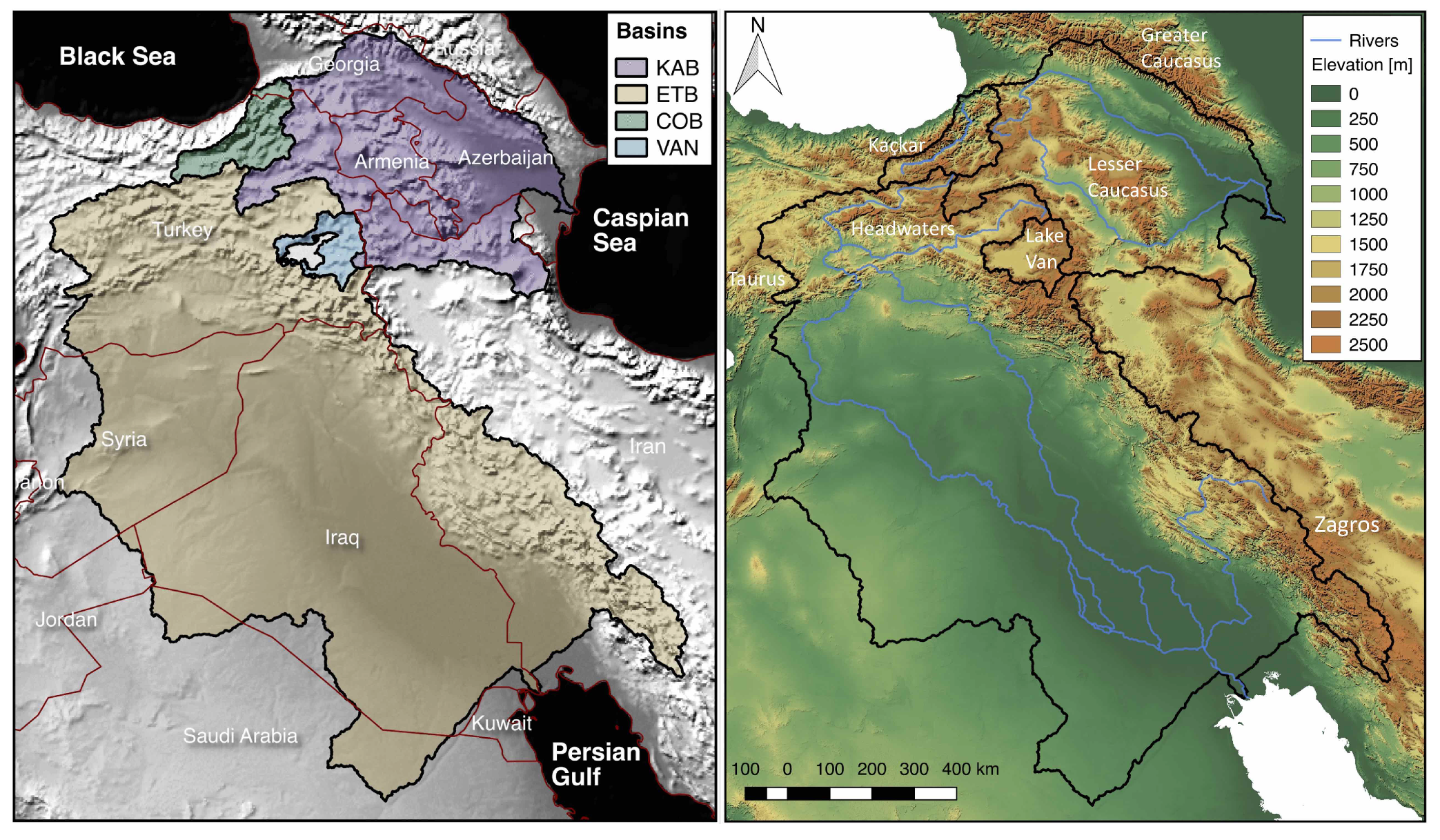
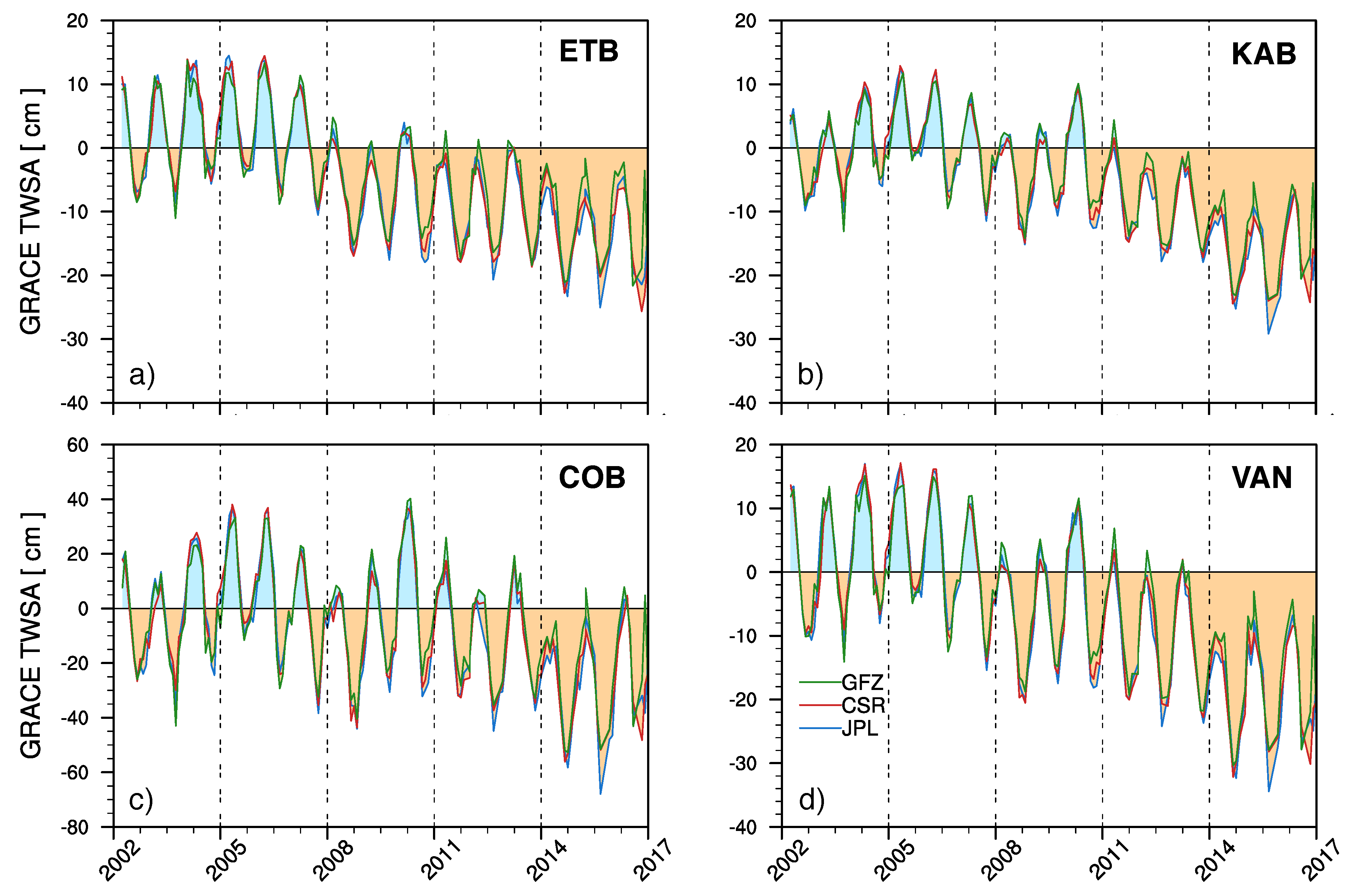
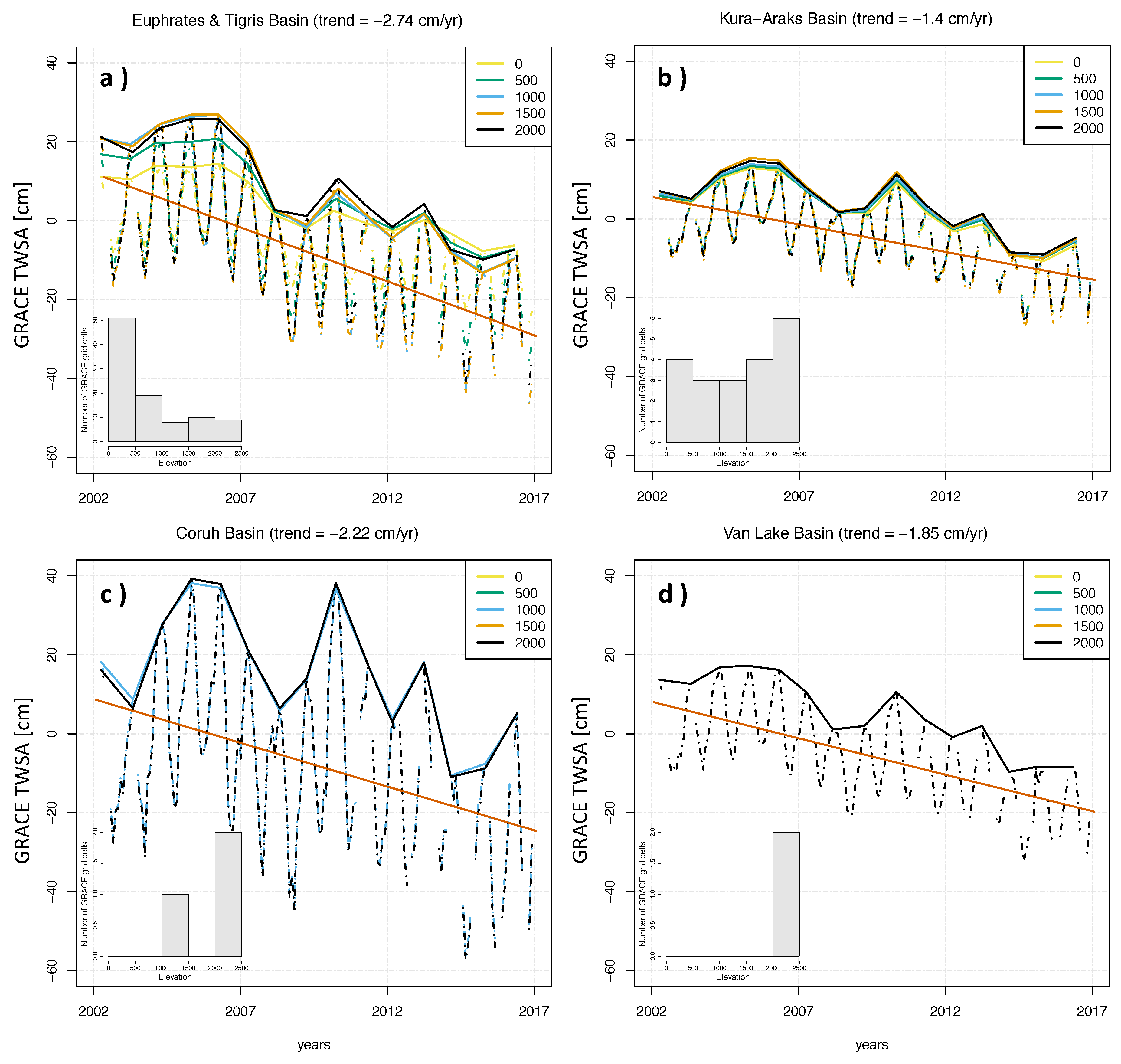
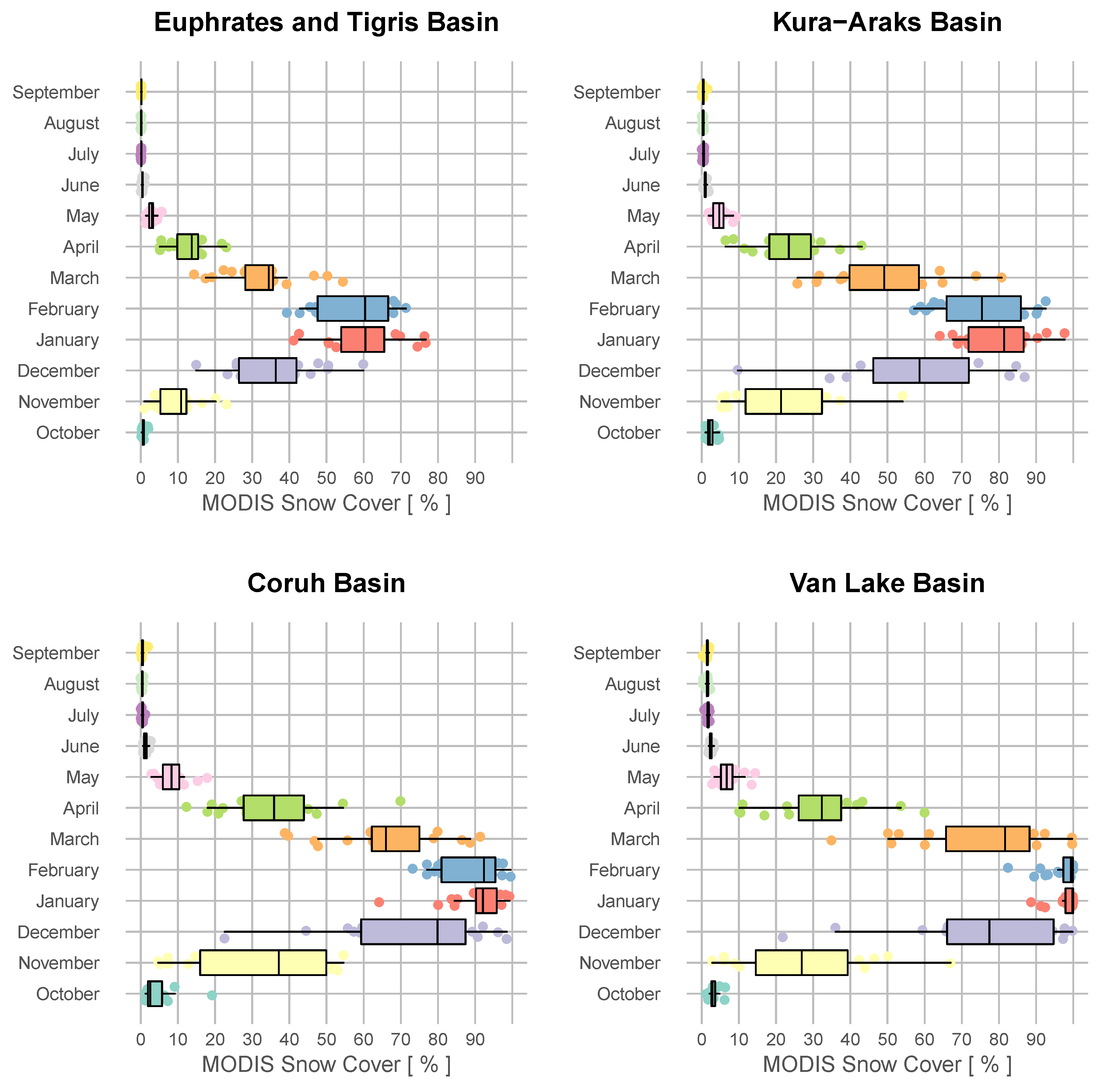
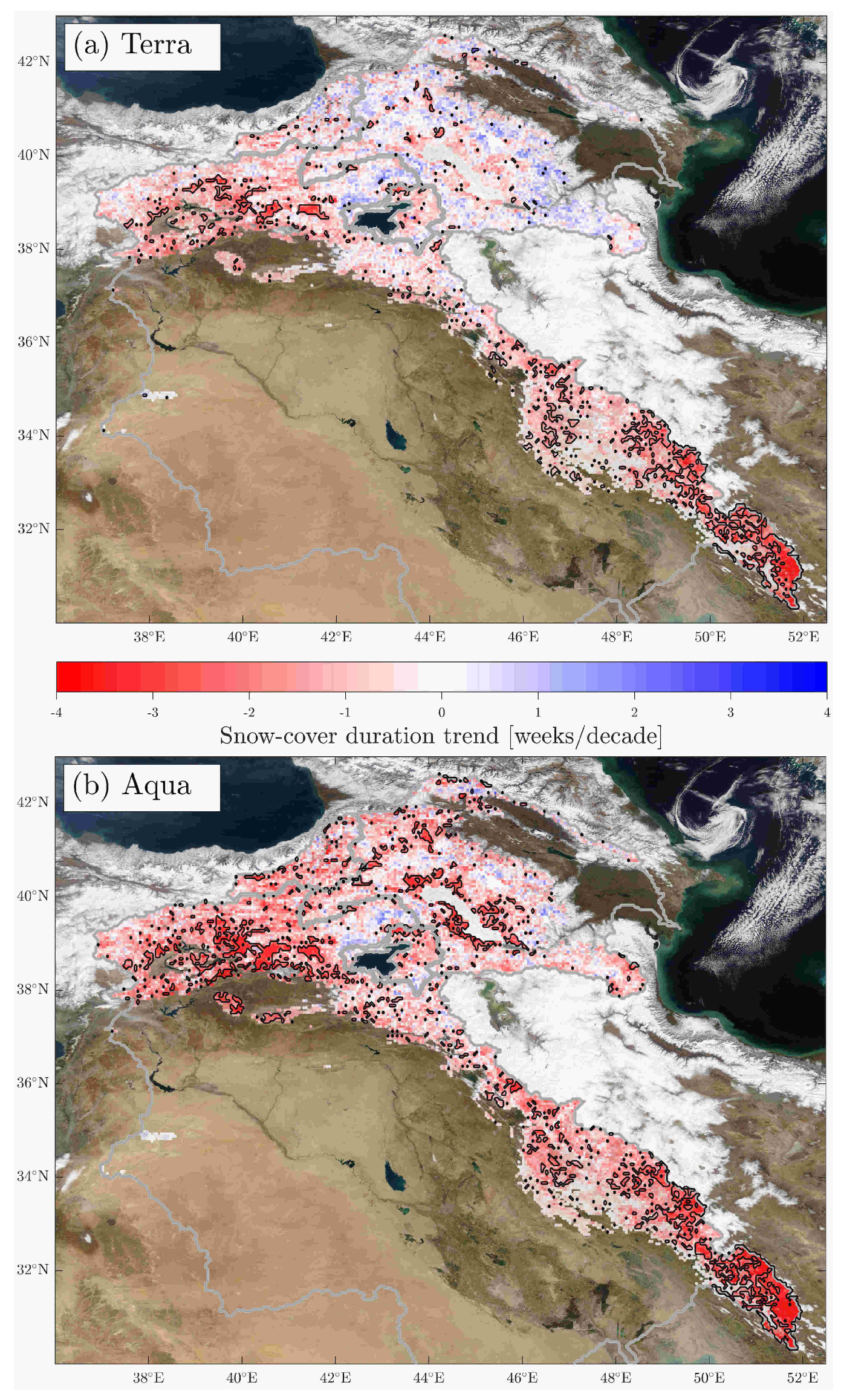
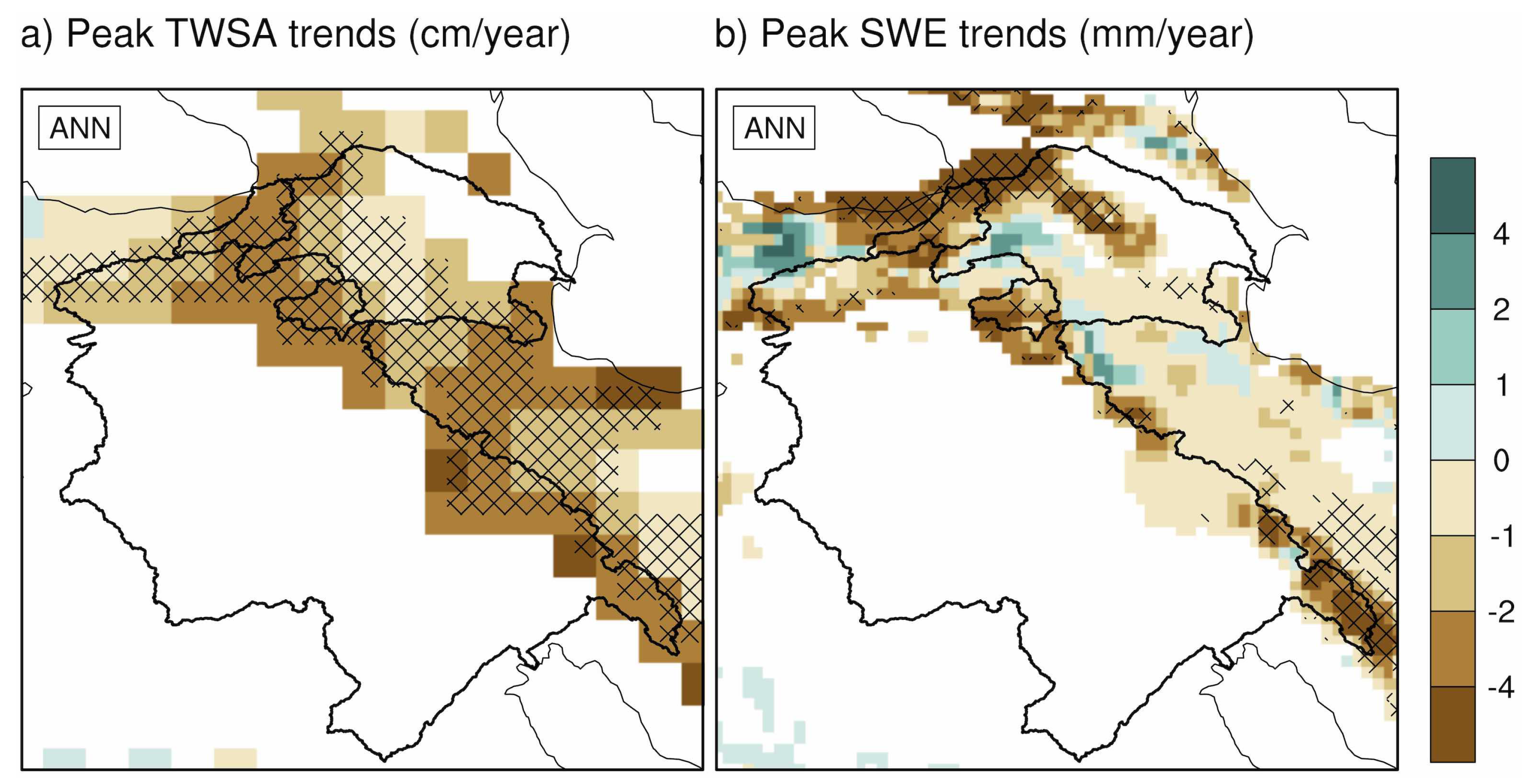
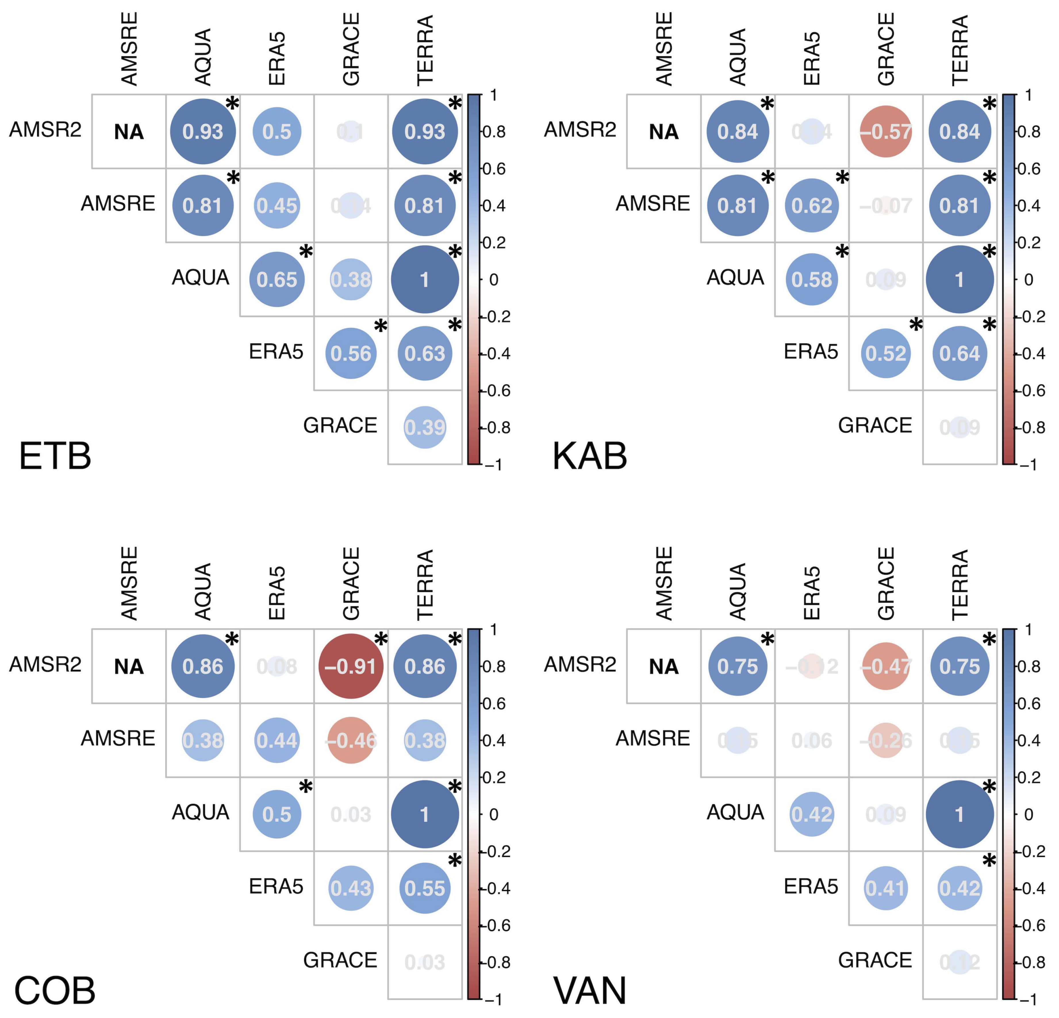
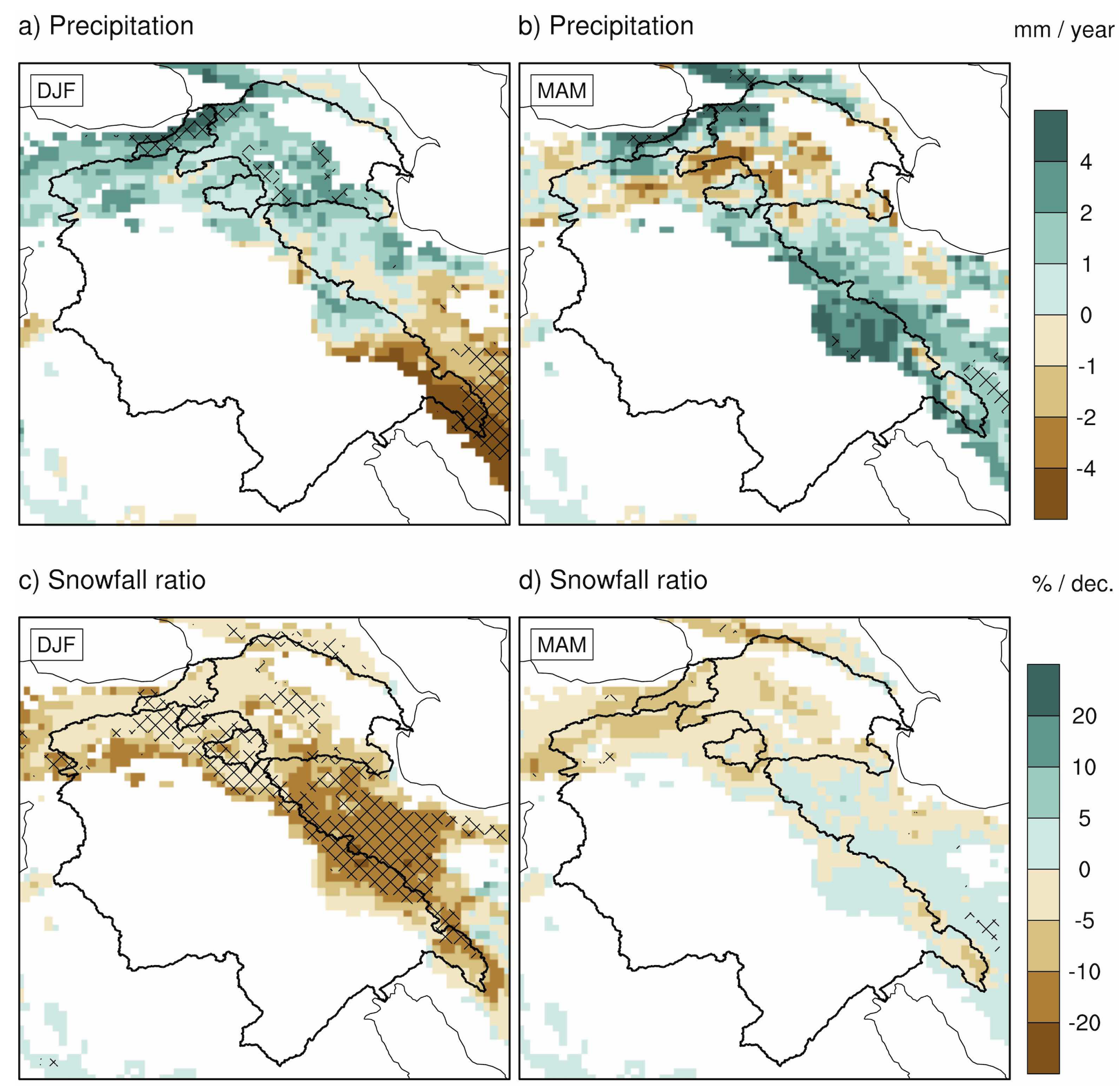
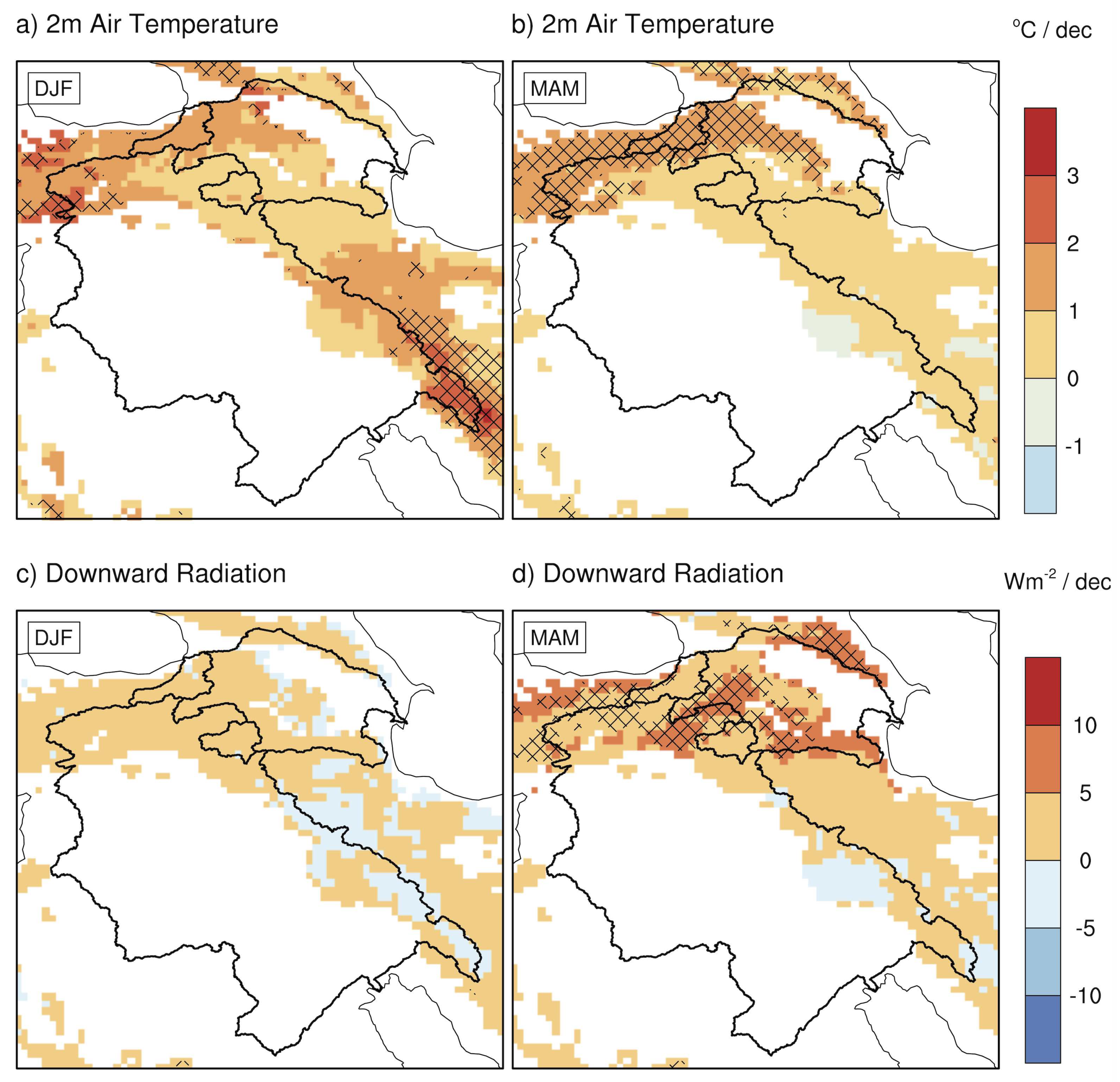
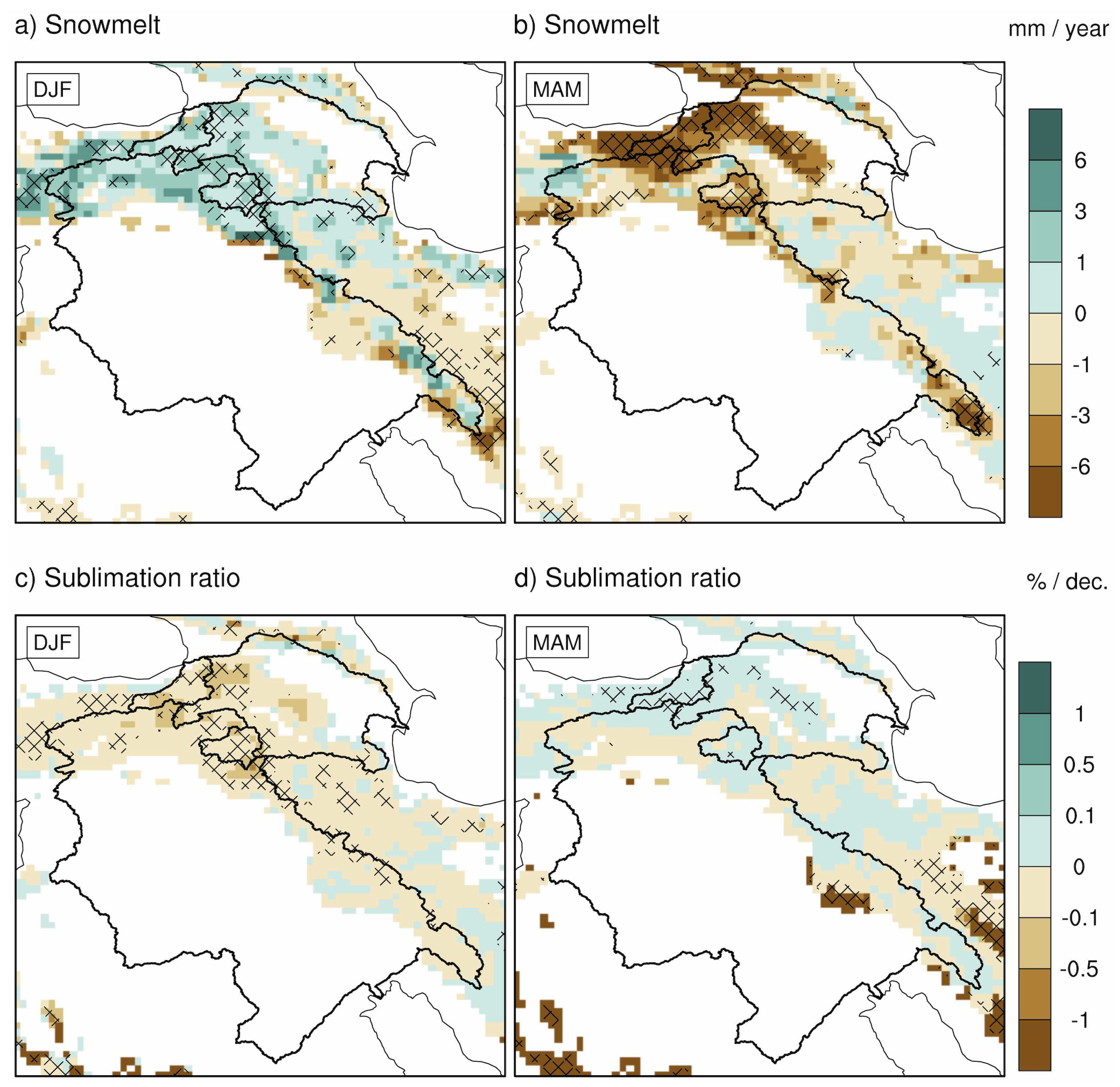
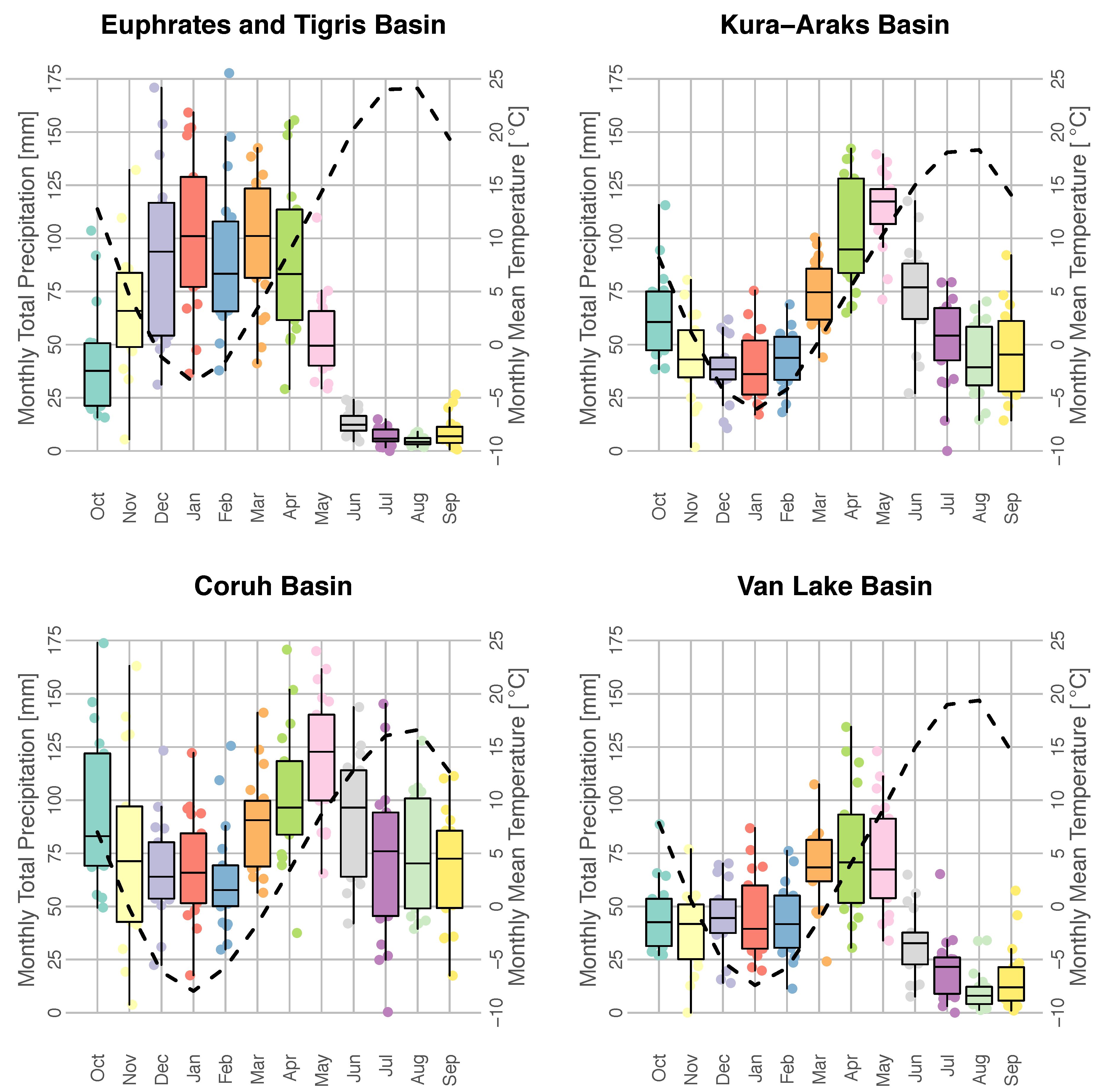
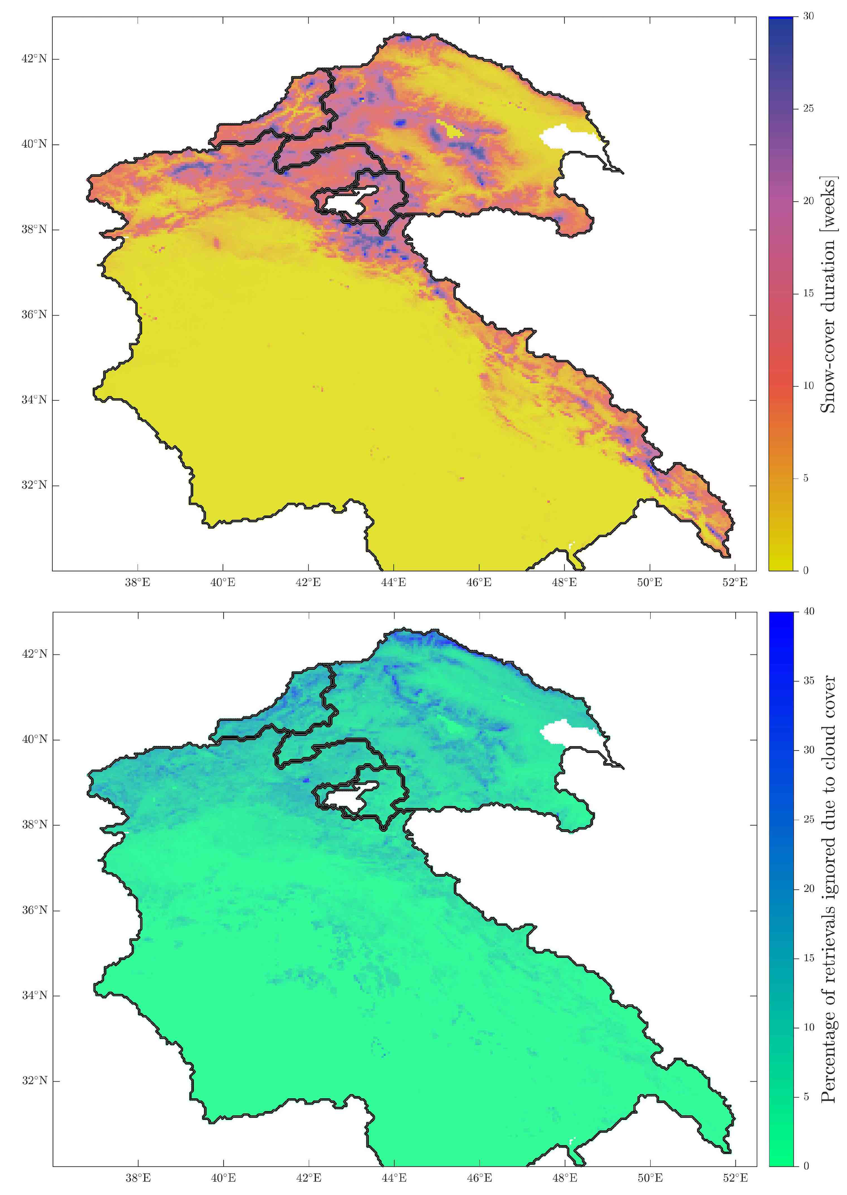
Table 1.
Geographic features of the study basins.
| Total Drainage Area (km) [61,68] | Mean Elevation from SRTM (m) | Precipitation ERA5 (mm/Year) | Riparian Countries (% of Total Area) [1] | |
|---|---|---|---|---|
| ETB | 868,060 | 734 | 326 | Iraq (46), Turkey (22), Iran (19), Syria (11), Saudi Arabia (1.9), Jordan (0.03) |
| KAB | 190,033 | 1330 | 665 | Azerbaijan (31.5), Iran (19.5), Georgia (18.2), Armenia (15.7), Turkey (15.1) |
| COB | 22,039 | 1842 | 1001 | Turkey (90), Georgia (10) |
| VAN | 17,915 | 2178 | 504 | Turkey (100) |
Table 2.
Description of the data sets used in this study.
| Data Set | Variable | Spatial Resolution | Temporal Coverage | Description |
|---|---|---|---|---|
| GRACE | Liquid water equivalent thickness anomaly (cm) | 1 | April 2002–January 2017 | gravimetric |
| Aqua MODIS | Snow-covered area (%) | 0.05 | July 2002–July 2018 | optical |
| Terra MODIS | Snow-covered area (%) | 0.05 | March 2000–July 2018 | optical |
| AMSR-E | Snow water equivalent (mm) | 25 (km) | June 2002–September 2011 | passive microwave |
| AMSR2 | Snow water equivalent Snow depth (mm) | 25 (km) | August 2012–July 2018 | passive microwave |
| SRTM30 | Elevation (m a.s.l.) | 0.0083 | February 2000 | radar |
| ERA5 | Snow energy and mass balance | 0.25 | January 2002–July 2018 | reanalysis |
Table 3.
Annual trends (unit/year) calculated from the results of a linear model applied to each elevation threshold for the different basins. The numbers in red show negative trends, while positive trends are in blue. Significance codes: 0.001 (****), 0.01 (***), 0.05 (**), 0.1 (*).
Table 3.
Annual trends (unit/year) calculated from the results of a linear model applied to each elevation threshold for the different basins. The numbers in red show negative trends, while positive trends are in blue. Significance codes: 0.001 (****), 0.01 (***), 0.05 (**), 0.1 (*).
| Data Set | GRACE | MODIS Aqua | MODIS Terra | ERA5 | AMSR-E | AMSR2 |
|---|---|---|---|---|---|---|
| Variable (Unit) | TWS (cm) | SCD (Days) | SCD (Days) | SWE (mm) | SWE (mm) | SWE (mm) |
| ETB | ||||||
| 0 m | −1.58 **** | −0.75 * | −0.50 | −0.49 | −0.36 | −0.76 |
| 500 m | −2.18 **** | −0.75 * | −0.50 | −1.02 | −0.65 | −1.45 |
| 1000 m | −2.84 **** | −1.15 * | −0.79 * | −1.6 | −0.84 | −2.56 |
| 1500 m | −2.84 **** | −1.19 * | −0.82 * | −1.65 | −0.96 | −3.64 |
| 2000 m | −2.53 **** | −1.49 ** | −1.06 ** | −2.96 ** | −1.44 | −4.36 |
| KAB | ||||||
| 0 m | −1.34 **** | −0.79 | −0.12 | −1.23 ** | −1.33 | 1.16 |
| 500 m | −1.32 **** | −0.79 | −0.12 | −1.51 ** | −1.54 | 1.36 |
| 1000 m | −1.33 **** | −0.79 | −0.12 | −1.71 ** | −1.76 | 1.4 |
| 1500 m | −1.39 **** | −0.69 | −0.06 | −2.07 ** | −2 | 1.18 |
| 2000 m | −1.32 **** | −0.79 | −0.15 | −2.41 ** | −1.67 | 1.88 |
| COB | ||||||
| 0 m | −1.92 ** | −1.1 | −0.39 | −5.52 *** | −2 | 2.22 |
| 500 m | −1.92 ** | −1.1 | −0.39 | −5.52 *** | −2.06 | 2.33 |
| 1000 m | −1.92 ** | −1.06 | −0.36 | −5.34 *** | −2.21 | 2.46 |
| 1500 m | −1.88 ** | −0.99 | −0.31 | −4.8 ** | −2.22 | 2.64 |
| 2000 m | −1.88 ** | −1.16 | −0.38 | −4.51 ** | −1.78 | 4.33 |
| VAN | ||||||
| 1500 m | −1.89 **** | −0.87 | −0.51 | −1.27 | 1.17 | −5.61 |
| 2000 m | −1.89 **** | −0.82 | −0.46 | −1.61 | 1.55 | −6.67 |
© 2019 by the authors. Licensee MDPI, Basel, Switzerland. This article is an open access article distributed under the terms and conditions of the Creative Commons Attribution (CC BY) license (http://creativecommons.org/licenses/by/4.0/).
Share and Cite
MDPI and ACS Style
Yılmaz, Y.A.; Aalstad, K.; Sen, O.L. Multiple Remotely Sensed Lines of Evidence for a Depleting Seasonal Snowpack in the Near East. Remote Sens. 2019, 11, 483. https://0-doi-org.brum.beds.ac.uk/10.3390/rs11050483
AMA Style
Yılmaz YA, Aalstad K, Sen OL. Multiple Remotely Sensed Lines of Evidence for a Depleting Seasonal Snowpack in the Near East. Remote Sensing. 2019; 11(5):483. https://0-doi-org.brum.beds.ac.uk/10.3390/rs11050483
Chicago/Turabian StyleYılmaz, Yeliz A., Kristoffer Aalstad, and Omer L. Sen. 2019. "Multiple Remotely Sensed Lines of Evidence for a Depleting Seasonal Snowpack in the Near East" Remote Sensing 11, no. 5: 483. https://0-doi-org.brum.beds.ac.uk/10.3390/rs11050483
Note that from the first issue of 2016, this journal uses article numbers instead of page numbers. See further details here.