A Multiscale Hierarchical Model for Sparse Hyperspectral Unmixing

1
School of Automation and Electrical Engineering, University of Science and Technology Beijing, Beijing 100083, China
2
Beijing Engineering Research Center of Industrial Spectrum Imaging, Beijing 100083, China
*
Author to whom correspondence should be addressed.
†
These two authors contribute equally to this work.
Remote Sens. 2019, 11(5), 500; https://0-doi-org.brum.beds.ac.uk/10.3390/rs11050500
Submission received: 26 January 2019
/
Revised: 15 February 2019
/
Accepted: 23 February 2019
/
Published: 1 March 2019
(This article belongs to the Special Issue Multispectral Image Acquisition, Processing and Analysis)
Abstract
:Due to the complex background and low spatial resolution of the hyperspectral sensor, observed ground reflectance is often mixed at the pixel level. Hyperspectral unmixing (HU) is a hot-issue in the remote sensing area because it can decompose the observed mixed pixel reflectance. Traditional sparse hyperspectral unmixing often leads to an ill-posed inverse problem, which can be circumvented by spatial regularization approaches. However, their adoption has come at the expense of a massive increase in computational cost. In this paper, a novel multiscale hierarchical model for a method of sparse hyperspectral unmixing is proposed. The paper decomposes HU into two domain problems, one is in an approximation scale representation based on resampling the method’s domain, and the other is in the original domain. The use of multiscale spatial resampling methods for HU leads to an effective strategy that deals with spectral variability and computational cost. Furthermore, the hierarchical strategy with abundant sparsity representation in each layer aims to obtain the global optimal solution. Both simulations and real hyperspectral data experiments show that the proposed method outperforms previous methods in endmember extraction and abundance fraction estimation, and promotes piecewise homogeneity in the estimated abundance without compromising sharp discontinuities among neighboring pixels. Additionally, compared with total variation regularization, the proposed method reduces the computational time effectively.

1. Introduction
Hyperspectral images possess abundant spectral information, which makes target detection and classification become feasible [1,2]. However, due to a low spatial resolution of hyperspectral sensor and the complex background, amounts of mixed pixels exist in the image and that makes it impossible to determine the material directly from the pixel level. In order to ensure the materials, called endmembers, in a scene, hyperspectral unmixing (HU) is being researched to solve the issue. Through the HU technique, we can identify the distinct endmember signatures that are present in a scene and its corresponding abundance fractions in each pixel. Thanks to the HU, this makes it possible for precision classification and target detection at the sub-pixel level for risk prevention and response [3,4,5].
Research work has been devoted to HU. Among it, non-negative matrix factorization (NMF) has been shown to be a useful unsupervised decomposition for hyperspectral unmixing [6]. The learned non-negative basis vectors that are used are distributed, yet they are still sparse combinations that generate expressiveness in the signal reconstructions [7]. Generally, NMF is attractive because it usually provides a part-based representation of the data, making the decomposition matrices more interpretable [8]. There are many possibilities to define the cost function and procedures for performing its alternating minimization, which leads to several improved NMF algorithms. The most popular algorithms for NMF belong to the class of multiplicative Lee–Seung algorithms, which have relatively low complexity but are characterized by slow convergence and risk becoming stuck in local minima [9]. To improve the performance of the NMF based hyperspectral unmixing method, further constraints were imposed on NMF [10,11,12,13,14]. Miao and Qi proposed a minimum volume constrained non-negative matrix factorization [15]. Sparsity constraints have gained much attention since most of the pixels are mixtures of only a few endmembers in the scene, which implies that the abundance matrix is a large degree of sparsity. Furthermore, regularization methods are usually utilized to define the sparsity constraint on the abundance matrix. Along these lines, L1/2 regularization is introduced into NMF so as to enforce the sparsity of the endmember abundance matrix [8]. However, the performance of many existing NMF algorithms may be quite poor, especially under the condition where the unknown nonnegative components are badly scaled (ill-conditioned data), insufficiently sparse, and a number of observations are equal or only slightly greater than a number of latent (hidden) components [16]. Therefore, a hierarchical strategy or multilayer NMF (MLNMF) is proposed to improve the performance of existing NMF, which is fully confirmed by extensive simulations with diverse types of data to blind source separation [16,17].
It should be noted that the phenomenon of spectral variability, which can be caused by variable illumination and environmental, atmospheric, material aging, object contamination, and other conditions, cannot be neglected [18,19,20,21,22]. It is shown that the same material spectra may be varied in the different area or the different materials may have similar spectra. Likewise, as the spatial resolution of imagery increases [23], it reduces the mixed pixel number in the image while increasing the spectral variability. Therefore, if we only extract the spectra from one of the areas as the endmember for unmixing, then the abundance map may not be accurate. To circumvent these issues, spatial regularization approaches, such as Total Variation Regularization (SUnSAL-TV), deserve special attention since they promote solutions that are spatially piecewise and homogeneous without compromising sharp discontinuities between neighboring pixels [24,25]. However, this adoption has come at the expense of a massive increase in computational cost and it needs the complete endmember matrix prior knowledge. On the other hand, it is worth considering that the hyperspectral image data acquired by different imagery sensors is various. Likewise, different optimal spatial resolutions exist for different object characteristics, suggesting for the need for a multiscale spatial approach for detection and analysis. In the literature [26], it has been proved that the spectral variability of land cover was reduced in coarser resolution images when compared to finer resolutions. Thus, it is essential to find a multiscale HU method to improve the unmixing accuracy regardless of the spatial resolution.
In this paper, a multiscale spatial regularization hierarchical model is considered to tackle the sparse unmixing problem. It breaks the unmixing problem into two domain problems. One is in an approximation domain that considers the spatial contextual information and the other is in the original domain that considers the detail information. Unlike the Total Variation Regularization that requires considering explicitly the dependences between pairs of pixels, the proposed multiscale regularization process compares the abundance matrix directly, which results in a computationally efficient procedure.
2. Theoretical Methodology
2.1. Linear Mixture Model
When using the linear mixture model, the following three assumptions apply: (1) the spectral signals are linearly contributed by a finite number of endmembers within each IFOV weighted by their covering percentage (abundance); (2) the land covers are homogeneous surfaces and spatially segregated without multiple scattering; (3) the electromagnetic energy of neighboring pixels do not affect each other [27,28]. Under the linear mixture model assumption, we have:
where M = [m1, …, mp] is the matrix of endmembers (mi denotes the ith endmember signature and p is the number of endmember, B is the band number), and S is the abundance matrix ([S]i,j denotes the fraction of the ith endmember of the pixel j and N denotes the total number of pixels), and denotes a source of additive noise. The abundance matrix needs every element within it, should be non-negative, and sum to one in each column.
2.2. Multiscale Hierarchical Unmixing Methods
The proposed multiscale hierarchical model for sparse hyperspectral unmixing method (MHS-HU) consists of two steps. First, we transform the original image domain (D) to an approximation (coarse) domain (C) using the multiscale method. Then we conduct the hierarchical sparsity unmixing (HSU) [22] method to obtain the endmember and abundance matrix to regularize the original unmixing problem. Different from the former method, the weighting matrix in this paper is set to the unit matrix. Superior to the HSU method, this procedure avoids the man-made endmember spectral variability library selection and estimation. On the other hand, it should be noted that the literature [24] also made the HU procedure in the coarse domain. However, compared with the literature [24] method, this paper uses a L1/2 norm to impose further sparsity, rather than using the L1 norm. In addition, we use multilayer sparsity to achieve better estimates of endmembers and abundance matrix results.
HU in the coarse domain can reduce the spectral variability effect.
Next, we apply a conjugate transformation to convert the abundance matrix obtained in the coarse domain before going back to the original image domain. The converted abundance matrix is then used to regularize the unmixing process to promote the spatial dependency between neighboring pixels. Then, with the abundance matrix constraints, we conduct the unmixing procedure again. Finally, we obtain the endmember and abundance matrix.
Consider a linear operator , that implements a spatial transformation of the original domain. Then,
where is the coarse domain of the original image Y. K denotes the total number of pixels in the coarse domain. The W matrix is upscaling matrix which reduces the image dimension and computational cost. Then the hierarchical sparsity unmixing procedure can be re-casted into the coarse domain. It can be computed as follows:
The value of the parameter depends on the sparsity of the material abundance and it is computed based on the sparseness criteria, shown as follows
where and are some constants to regularize the sparsity constraints, and denotes the iteration number in the process of optimization [16]. Then we obtain the estimated abundance matrix in the coarse domain. We define a conjugate transform , which converts the images from the coarse domain back to the original domain:
where is the smooth approximation of the abundance in the original domain, which can be used to regularize the original unmixing problem. In this way, it is possible to introduce a spatial correlation into the abundance map solutions by separately controlling the regularization strength in each of the coarse and original domain. Compared with the traditional total variation regularization [25] that requires to consider explicitly the dependences between all pairs of pixels, the proposed method considering the dependences between the two abundance matrices can reduce time consuming computational cost.
Following this idea, we define the multiscale hierarchical model for sparsity unmixing method as follows:
where is a regularization parameter. Since the SD obtained in the coarse domain is invariant in this equation, the additional item is still convex. Note that compared with the hierarchical sparsity unmixing method in the coarse domain, the update rule for the endmember matrix stays invariant, while the update rule for the abundance matrix must be different. Now we address the update rule for the abundance matrix S. To make our elaboration clearer, the objective function is separable in the columns of S. Likewise, the corresponding row of Y is denoted y. The column-wise objective function becomes
2.2.1. Multiscale Methods
Large volumes of high-resolution hyperspectral image data offer challenges that are more time-consuming, complex, and computationally intensive than a single scene analysis to the user. In addition, in high resolution hyperspectral image data, the spectral variability phenomenon is also obvious, which restricts the unmixing accuracy. However, there are amounts of mixed pixels in the low spatial hyperspectral image. Balancing the effect of the mixed pixel and spectral variability, using the multiscale unmixing method to interpret each pixel can no doubt improve the classification accuracy [29]. That is reasonable because the multiscale strategy considering the surrounding pixels reduces the spectral variability effect. Additionally, as a rule of thumb, each object has its suitable scale to be detected [26]. Using high resolution hyperspectral image data makes it possible to provide multiscale analysis.
In multiscale methods, nearest-neighbor (NN), bilinear interpolation (BIL) and cubic convolution (CC) are commonly available in a commercial image processing software package [30]. In NN, the DN of the pixel closest to the location of the original input pixel is assigned to the ones at the output pixel location. In BIL, the DN is assigned to the output pixel by interpolating DNs in two orthogonal directions within the input image. Essentially, it also can be computed based on the weighted distances to the points. In CC, the weighted DN values of 16 pixels surrounding the location of the pixel in the input image are used to determine the value of the output pixel.
However, as illustrated in the literature [30,31], the nearest neighbor, bilinear interpolation, and cubic convolution resampling methods are not suitable for resampling remotely sensed data. And the results showed that both Gaussian and aggregation resampling methods were found to produce similar radiance values [26]. In the literature [32], the study showed that compared with other aggregation resampling methods, a point-centerd distance-weighted moving window (PDW) is the best option to be used in, for example, the studies on ecological resource management where consistency of the class proportions at coarser resolutions is required. Therefore, for convenience, no weighting PDW is used in this study.
2.2.2. The Optimization Problem
To guarantee the convergence of the update rule, we define an auxiliary function G(s, st) satisfying the condition G(s, s) = and G(s, st) such that is a non-increasing function when updated using the following equation
This is guaranteed by
The Taylor expansion of can be written as
We define the function G as
where the diagonal matrix K(st) is
Then
To improve performance in solving the Equations (3) and (6), especially for ill-conditioned or badly scaled data, and reducing the risk of getting stuck in the local minima of a cost function, we develop a hierarchical procedure in which we perform a sequential decomposition of non-negative matrices for hyperspectral unmixing. The mathematical representation of the hierarchical structure is formulated as
where the l denotes the layer number. Thus, the endmember and abundance matrix in each layer, and , can be achieved by a modification of the multiplicative update rules as follows.
Furthermore, regarding the sum-to-one constraint on the abundance fraction in the model (1), the data matrix and the endmember matrix are augmented by a row of constants defined by
where controls the impact of additivity constraint over the endmember abundance fractions, and N and p denote the whole pixel number and endmember number, respectively. The larger the , the closer the sum over the columns of the abundance matrix are to unity. In each layer iteration, these two matrices are taken as the input of the update rule in Equations (16) and (17) as an alternative to Y and M.
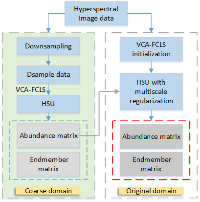
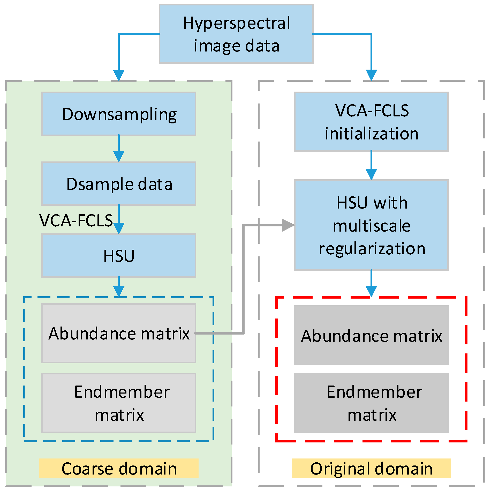
Figure 1 shows the flowchart of the proposed method. The abundance and endmember matrix in blue dotted line are the outputs of the coarse domain. And the matrices in the red dotted line are the final outputs of the method.
3. Experiments
3.1. Experimental Data
In this section, we introduce two sets of experimental data, simulated data, and real image data.
The simulated data makes it possible for presetting the endmember set and abundance fraction map as prior knowledge that can be used as a measurement for the approach performance. The procedure described in the literature [15] has been used to create the simulated data. In this paper, the simulated data endmember spectra are derived from the USGS digital library. The data set is a 224 spectral band image with n = 2000 pixels consisting of five endmembers. The endmembers are extracted from the USGS library randomly. The abundance maps are piecewise smooth images. In addition, the variety of spectral features and different signal-to-noise ratios have been employed to generate the simulated images. To ensure no pure pixel exists, all the abundance fractions larger than 0.8 are discarded. To make the scenes more realistic and reasonable, white Gaussian noise is added and SNR is set to 30 dB [3].
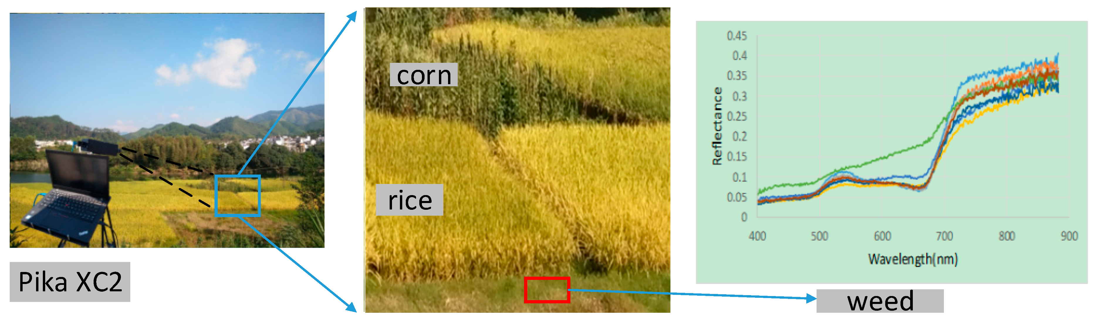
Apart from the simulated data, we also conduct a real data experiment. There are two real data cubes. The first real hyperspectral image data cube, RC1, we choose the data obtained by ground-based hyperspectral imaging instrumentation. The experiment site is located in Wuyuan (29.35°N; 118.09°E), Jiangxi province, China. The images are captured by a Pika XC2 imaging of Resonon, which is a push broom imager designed for the acquisition of visible and near-infrared hyperspectral images ranging from 400 nm to 1000 nm with 1.3 nm spectral resolution in September 2017 [22]. The image was calibrated using a white reference panel and converted from radiance to reflectance. The original image has 462 channels. Note that channels 1–13 and 385–462 were blurred due to the sensor noise and atmospheric water vapor absorption. As a result, we only used channels 13–384 with the wavelength ranging from 400 nm to 900 nm. Therefore, the size of the test image is 400 × 400 × 372. Rice, grass, and corn are in the scene, shown in Figure 2. The right curve plot displays an example of the spectral variability of the weed. Each spectrum is collected in a different area.
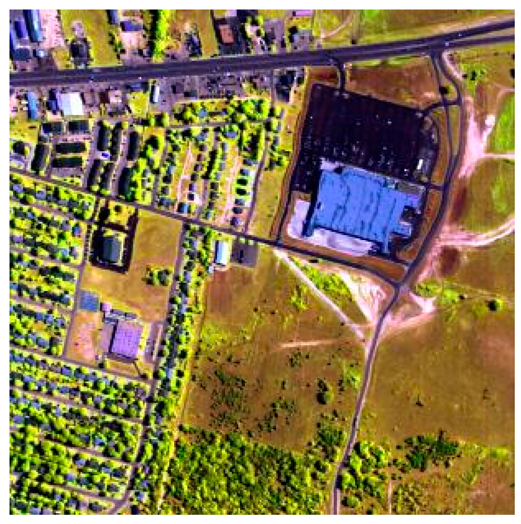
The second real data cubes, RC2, is the classic hyperspectral data, Urban, collected by HYDICE hyperspectral imagery. The size of the image is with a spatial resolution of 2 m. It contains 210 spectral channels with the spectral resolution of 10 nm in the 400 nm and 2500 nm range. The imaging area is located at Copperas Cove near Fort Hood, TX, U.S. After removing low SNR and water-vapor absorption bands, a total number of 162 bands remained. The five materials prominently present in RC2 are asphalt, grass, roof, shadow and tree. The false color of the RC2 is displayed in Figure 3.
For the evaluation of the proposed method, spectral angle distance (SAD), abundance angle distance (AAD), root mean square error (RMSE) and abundances mean squared error (MSEa) are used in this paper. It should be noted that the endmembers of the synthetic data are extracted from USGS serving as the reference endmembers. For the real image data, the reference endmembers are extracted from the image. Each endmember class is extracted from the pure pixel area. Then an average of the observations in each endmember class is computed, serving as reference endmember spectra.
SAD is defined as:
where mi denotes the ith endmember spectra, <mi, mj> denotes the inner product of the two spectra, denotes the vector magnitude. It is used to compare the similarity of the original pure endmember signatures and the estimated ones.
AAD is used on the condition that the abundance fractions are known as prior knowledge. It measures the similarity between original abundance fractions (si) and the estimated ones (), which is formulated in the equation below.
To obtain an overall measure accuracy, root mean square of these measures are defined as
where p denotes the number of endmember and N denotes the whole number of pixels.
RMSE is denoted by
where N denotes the total number of pixels, B denotes the total number of spectral bands, and denotes the error of the ith row and the jth column between the original and simulated image data. It is used to evaluate the reconstruction estimates’ error. Since the model errors are likely to have a normal distribution rather than a uniform distribution, the RMSE is a good metric to present model performance [33].
MSEa is denoted by
where N denotes the total number of pixels, p denotes the endmember number, and M denotes the original endmember matrix, denotes the estimated endmember matrix. It is used to evaluate the abundance estimates’ error. MSEa is used on the condition that the truth endmember is known as prior knowledge.
3.2. Simulated experiments
In the simulated experiment, the parameters of the algorithm are set as follows: , the window scale is five and the maximum iteration time is 1000. In this experiment, SNR is set to 25 dB. Figure 4 shows the proposed method, MLNMF, L1/2-NMF, VCA-FCLS and SUnSAL-TV [25,34,35] method unmixing results, respectively. The selection of these algorithms comes naturally since the proposed methods, L1/2-NMF and SUnSAL-TV, share similar sparse regression formulations [8,24], and MLNMF [17] also considers the multilayer strategy to improve the existing NMF performance. VCA-FCLS is the traditional method and is also used as the initial unmixing method, which results in the inputs of the proposed method. It should be noted that the SUnSAL-TV is only an abundance estimation method that needs the endmember matrix input as prior knowledge. Therefore, we input the endmember extracted by the VCA to the SUnSAL-TV. The input parameters used in SUnSAL-TV are λ = 0.01 and λTV = 0.001. The first column demonstrates the original simulated abundance fraction, and the second column to the sixth ones are corresponding to the abundance fraction map estimated by different methods, respectively. The abundance fraction map is denoted using a color bar, which the blue color shows the least fraction near to zero and the red color shows the highest fraction near to one. The variation of color bar is consistent with the natural spectral wavelength change. From the figure, it is obvious that the proposed method can obtain a higher precision in abundance estimation than the traditional single layer L1/2-NMF algorithm. Table 1 shows the true and reconstructed abundance maps for the different algorithms. The compared methods are L1/2-NMF, MLNMF, VCA-FCLS and SUnSAL-TV. As expected, models accounting for hierarchical or multilayer strategy tend to yield better reconstruction quality than L1/2-NMF. The proposed method yields the smallest abundance reconstruction error, followed by MLNMF. The discrepancies between the MSEa and RMSE results among the methods that address spectral variability indicate that there is no clear relationship between these two variables. This is due to the fact that the MSEA pays more attention to the abundance estimates, while RMSE focuses on the reconstruction error of the image data. Additionally, the proposed method considers the spatial regularization as the additional constraints, therefore it tends to yield more stable unmixing results compared with the MLNMF. In terms of computational cost, we compared the proposed method with the SUnSAL-TV. The computational complexity of the algorithms is evaluated through the average execution time of 20 runs, which is displayed in Table 2. The results show that the proposed method performed significantly better than the SUnSAL-TV, with execution times 7 to 12 times smaller than the SUnSAL-TV. That is due to the fact that the proposed method tends to compare the dependences between the two domain abundance matricies rather than all pairs of pixels that reduce the computational cost.
In addition, to verify how the multiscale window affects the proposed method in hyperspectral unmixing accuracy, we experiment with various window scale and the coefficient beta under the same fixed initial condition. Both the statistics are based on the average value of thirty times running results. Table 3 shows the various window scale comparison results. It is observed that the performance does not vary significantly from its optimal values unless the window becomes too large. This is reasonable that when the window becomes too large, it may produce a higher mixture pixel that increases the difficulty of the inverse solution. Furthermore, Table 4 illustrates the weighting coefficient of the multiscale effect on the final unmixing accuracy. As the results show, tends to obtain better results.
Therefore, we have illustrated the advantages of our proposed method on simulated data against L1/2-NMF, MLNMF, SUnSAL-TV and VCA-FCLS. The experimental results consistently show that MHS-HU exhibits better performance in hyperspectral unmixing. This is particularly true in the presence of ill-conditioned or projected gradient algorithms.
3.3. Real Data Experiments
In the first real data, RC1, experiment, the endmember and layer number are set as 3 and 4, respectively. The iteration in each layer is set to 1000. Furthermore, we set and the multiscale as 5.
Figure 5 shows the unmixing results of the proposed method and the compared methods. The compared methods are MLNMF, VCA-FCLS, SUnSAL-TV and L1/2-NMF. It is worth mentioning that both the spatial and spectral resolution of the image are so tiny that they capture the shadow details among the rice and corn. Furthermore, except for the spectral variability of crops especially caused by the shadow effect, the high similarity of corn and weed also increases the difficulty in vegetable abundance estimation. That is the reason why traditional unmixing methods such as VCA-FCLS and L1/2-NMF cannot produce the expected results in the vegetable abundance estimation, especially in rice abundance estimation. However, in this case, the proposed method shows significantly better performance estimating the rice abundance map when compared with the other algorithms. This indicates that the proposed method effectively exploits the spatial properties of the abundance maps by using multiscale strategy, resulting in more spatially consistent estimates with fewer outliers resulting from the influence of measurement noise. In addition, a hierarchical sparsity strategy is also used to search the optimal global solution. Thus we can obtain a better result than the traditional one, especially in distinguishing corn and rice. In the corn abundance map, all the methods made the wrong estimation and some weeds showed a high fraction. That is because the corn and the weed spectra are too similar in the visible waveband to distinguish them. Nevertheless, the proposed method can still estimate the corn abundance completely compared with the others. Table 5 illustrates the unmixing results of different methods. As mentioned before, the proposed method also outperforms other methods.
Table 6 illustrates the multiscale effect on the unmixing results. As expected, as the window scale varies, the accuracy increases to some degree. But when the window scale is too large, the accuracy tends to decrease. In this experiment, it should be noted that when the scale window is 1, it cannot be regarded as the original domain, such as in MLNMF. On the contrary, it means we conduct two continuous hierarchical sparsity hyperspectral unmixing procedures on the original domain, but with the first abundance result as the spatial regulation constraint of the second one. This tends to yield more stable results.
In the second real data experiment, the layer number is 4 and the maximum iteration time in each layer is 1000. Furthermore, we set α = 0.1, and τ = 10. The endmember number is set as 5 and the multiscale is 5. Since the true abundance maps are unavailable for the images, we make a qualitative assessment of the recovers abundance maps based on knowledge of materials present in a prominent fashion in those scenes. The major endmember abundance maps for the Urban data set are depicted in Figure 6. The compared methods are geometric-based VCA with FCLS, MLNMF and L1/2-NMF. As can be seen, the proposed method yields the best results for the overall abundances of all materials. Especially the roof abundance map, it corresponds with ground truth well. Not only the fraction of the biggest roof is near to 1, shown in red color, but also the other small size roof can also be estimated accurately. Also, in the tree abundance map, the proportion of the proposed method outperforms the other unmixing methods. Regarding the abundance map, Table 7 and Table 8 show the SAD and RMSE of different methods. The SAD results varied among the algorithms, with no method performing uniformly better than the others. Table 7 indicates that the proposed method and the MLNMF results are very close and significantly smaller than those of the other methods, which agrees with their better abundance estimation results. This falls in line with the fact that compared with the single layer L1/2-NMF, the hierarchical or multilayer NMF with abundance sparsity representation in each layer aims to obtain the global optimal solution [17]. On the other hand, since the grass and the tree have highly similar diagnostic spectral features, the grass and the tree cannot be endmember sets simultaneously in the geometric simplex [36]. This is why the traditional geometric based VCA-FCLS method cannot distinguish them effectively. Therefore, the proposed method and the MLNMF outperform the traditional methods. It should be noted that compared with MLNMF, the proposed method does not show the same advantage of using the multiscale strategy to improve the unmixing accuracy as the RC1 data experimental results. That is due to the fact that the Urban dataset is one of the prevalent authentication data for unmixing, which means every pixel in the dataset is well calibrated. The data is collected from the airborne imagery with nadir, observing that the shadow effect within the endmember class is much smaller than the RC1. In addition, the area is homogeneous. Thus, compared with the RC1 data cube, the spectral variability phenomenon is not obvious in this dataset. Table 9 shows the results versus various window scales. As mentioned before, the spatial resolution of RC2 data is 2 m and each endmember class is homogeneous with a large area and less spectral variability. The unmixing accuracy increases with the window scale to some degree. When the window scale becomes too large, the unmixing result deviates its optimal value. This is expected since the large multiscale size hinders the capability of transformation matrix W to capture coarse scale information [24]. Therefore, the best results are obtained with a proper window scale. To summarize, the results mentioned above confirm the satisfactory performance of the proposed method in terms of unmixing quality.
4. Discussion
Previous work has documented the effectiveness of various unmixing algorithms, especially in synthetic data. It should be noted that synthetic data is generated in a fully controlled environment, and the accuracy of the unmixing results can be effectively validated. However, it is not easy to realistically simulate the data close to the real data, which consists of various spectral variability. That is the reason why the unmixing results based on simulated data are often inconsistent with the ones based on real data. Notably, when it comes to verifying the endmember extraction accuracy, we tend to extract the spectra directly from the image by averaging the selected sample. Therefore, regarding the idea, this study decomposes the HU into the coarse and original domain to reduce the spectral variability effect.
As a rule of thumb, coarser spatial resolutions can result in a loss of spatial and spectral information. Amounts of studies have examined the impact of spatial resolution on the mapping of vegetation [26]. The results have indicated that a pixel size of 6 m or less would be optimal for studying the functional properties of southern California grassland [37]. However, considering the current conditions for the satellite hyperspectral imagery, it is hard to obtain a finer spatial resolution than 6 m. In this case, to improve the mapping accuracy, the unmixing procedure is in need. Since the demonstrated viability of upscaling approaches suggests that current ground instrumentation is adequate for satellite mission validation needs, it is also possible that new ground measurement technologies could significantly expand the spatial support of observations derived from ground-based instrumentation. Therefore, by resampling the ground-based or airborne images to coarser spatial resolutions and applying unmixing modeling algorithms, the impacts of spatial resolution on fraction estimation can be simulated. In addition, high resolution reference images can also be used for the validation of global land cover datasets. The accuracy assessment of the land surface parameters estimation algorithm is difficult to achieve due to the difficulties in obtaining actual fraction vegetation cover from the field surveys [38]. For this purpose, it is necessary to aggregate the high resolution reference map to the corresponding coarse resolution global land cover dataset [32]. Additionally, it is more persuadable to verify the unmixing result accuracy and saves much time or cost for the situ survey.
However, it should be noted that each material has its own fit resolution to be detected. Therefore, when we use the multiscale unmixing method, the multiscale window cannot be too large. Analogously, the literature [24] used superpixel algorithms for multiscale transformation, and it also mentioned that the performance might deviate, which is optimal value if the superpixel size became too large. This is expected since very large multiscale sizes may contain semantically different pixels, hindering the capability of the transformation in matrix W to adequately capture coarse scale information. Furthermore, the unmixing results for super resolution mapping (SRM) can also be used in a wide range of applications. Providing a map at the sub-pixel level is more persuadable than the simply fractional images. As illustrated in the literature [39], in this study both the unmixing method and the SRM were focused on developing the boundary of the river at the sub-pixel. On the other hand, compared with the SUnSAL-TV method using the endmember matrix as input, the proposed method can obtain the endmember and abundance matrix simultaneously without prior knowledge. In addition, the proposed method tends to compare the two domain abundance matrices rather than all the pixels that reduce the computational time.
Rather, it is impossible for the HU method results to maintain consistency under the various spatial resolution conditions. In this case, the users only pay more attention to which kind of HU method outperforms the others regardless of the spatial resolution or which spatial resolution is fit for the specific application. Therefore, it is feasible that the HU method using a multiscale unmixing strategy can consider the different spatial resolutions and enhance the stability of the results with spatial regularization.
5. Conclusions
This paper proposes an unsupervised multiscale hierarchical sparsity unmixing method to improve the accuracy of hyperspectral unmixing. It decomposes large scale spatially regularized sparse unmixing into two domain problems in different image domains, one capturing coarse domains and another representing fine scale details. Considering the spatial contextual information with an abundance matrix regularization in a coarse domain, the proposed method leads to a simple and efficient strategy to deal with spectral variability, especially caused by shadow between neighboring pixels. The unmixing procedure can then be solved at a reasonable computational cost. Additionally, it uses a hierarchical strategy to decompose matrices into a multilayer. In each layer, we force an abundance sparsity representation to improve the performance in hyperspectral unmixing. The proposed method has been applied to simulated and real datasets. Compared with MLNMF, SUnSAL-TV, L1/2-NMF and other approaches, the proposed method produces promising results in endmember extraction and abundance fraction estimation. Furthermore, it reduces the computational time effectively compared with SUnSAL-TV. It also considerably improves the unmixing performance especially if a problem is ill-conditioned. In addition, the projected gradient algorithms are used to reduce the risk of getting stuck in local minima. Furthermore, the proposed method can be readily applied to other conditions in which nonnegative sparse matrix factorization is a valuable computational tool. Additionally, it is worth mentioning that it may be more appropriate to focus future sensor development towards collecting data at the finest spatial resolution, and develop algorithms focused on upscaling routines, rather than collecting a host of different spatial resolution data with high expense cost. Thus, it is essential to find an appropriate upscaling technique to represent the hyperspectral data at different scales and a stable multiscale HU method in further research.
Author Contributions
J.Z. and J.L. are equally with contribution.
Funding
This research was funded by Major Special Project of the China High-Resolution Earth Observation system, the Funding 41416040203, and the Funding FRF-GF-18-008A.
Acknowledgments
We would like to thank the editor and reviewers for their reviews that improved the content of this paper.
Conflicts of Interest
The authors declare no conflict of interest.
References
- Zhang, Y.; Wu, K.; Du, B.; Zhang, L.; Hu, X. Hyperspectral target detection via adaptive joint sparse representation and multi-task learning with locality information. Remote Sens. 2017, 9, 482. [Google Scholar] [CrossRef]
- He, Z.; Wang, Y.; Hu, J. Joint sparse and low-rank multitask learning with laplacian-like regularization for hyperspectral classification. Remote Sens. 2018, 10, 322. [Google Scholar] [CrossRef]
- Bioucas-Dias, J.M.; Plaza, A.; Camps-Valls, G.; Scheunders, P.; Nasrabadi, N.; Chanussot, J. Hyperspectral remote sensing data analysis and future challenge. IEEE Geosci. Remote Sens. Mag. 2013, 1, 6–36. [Google Scholar] [CrossRef]
- Gevaert, C.; Suomalainen, J.; Tang, J.; Kooistra, L. Generation of spectral-temporal response surfaces by combining multispectral satellite and hyperspectral uav imagery for precision agriculture applications. IEEE J. Sel. Top. Appl. Earth Obs. Remote Sens. 2015, 8, 3140–3146. [Google Scholar] [CrossRef]
- Ma, D.; Yuan, Y.; Wang, Q. Hyperspectral Anomaly Detection via Discriminative Feature Learning with Multiple-Dictionary Sparse Representation. Remote Sens. 2018, 10, 745. [Google Scholar] [CrossRef]
- Huang, R.; Li, X.; Zhao, L. Hyperspectral unmixing based on incremental kernel nonnegative matrix factorization. IEEE Trans. Geosci. Remote Sens. 2018, 11, 6645–6662. [Google Scholar] [CrossRef]
- Hoyer, P.O. Non-negative matrix factorization with sparseness constraints. J. Mach. Learn. Res. 2004, 5, 1457–1469. [Google Scholar]
- Qian, Y.; Jia, S.; Zhou, J.; Robles-Kelly, A. Hyperspectral unmixing via L1/2 sparsity-constrained nonnegative matrix factorization. IEEE Trans. Geosci. Remote Sens. 2014, 49, 4282–4297. [Google Scholar] [CrossRef]
- Lee, D.D.; Seung, H.S. Algorithms for non-negative matrix factorization. In Proceedings of the International Conference on Neural Information Processing Systems, Denver, CO, USA, 29 November–4 December 2000; MIT Press: Cambridge, MA, USA, 2000. [Google Scholar]
- Ma, W.; Bioucas-Dias, J.; Chan, T.; Gillis, N. A signal processing perspective on hyperspectral unmixing: Insights from remote sensing. IEEE Signal Process. Mag. 2014, 31, 67–81. [Google Scholar] [CrossRef]
- Fang, H.; Li, H.C.; Li, J.; Du, Q.; Plaza, A.; Emery, W.J. Sparsity-constrained deep nonnegative matrix factorization for hyperspectral unmixing. IEEE Trans. Geosci. Remote Sens. 2018, 10, 6245–6257. [Google Scholar] [CrossRef]
- Wang, M.; Zhang, B.; Pan, X.; Yang, S.Y. Rank Nonnegative Matrix Factorization with Semantic Regularizer for Hyperspectral Unmixing. IEEE J. Sel. Top. Appl. Earth Obs. Remote Sens. 2018, 4, 1022–1029. [Google Scholar] [CrossRef]
- Zhang, Z.; Liao, S.; Zhang, H.; Wang, S.; Wang, Y. Bilateral Filter Regularized L2 Sparse Nonnegative Matrix Factorization for Hyperspectral Unmixing. Remote Sens. 2018, 10, 816. [Google Scholar] [CrossRef]
- Shao, Y.; Lan, J.; Zhang, Y.; Zou, J. Spectral Unmixing of Hyperspectral Remote Sensing Imagery via Preserving the Intrinsic Structure Invariant. Sensors 2018, 18, 3528. [Google Scholar] [CrossRef] [PubMed]
- Miao, L.; Qi, H. Endmember extraction from highly mixed data using minimum volume constrained nonnegative matrix factorization. IEEE Trans. Geosci. Remote Sens. 2007, 45, 765–777. [Google Scholar] [CrossRef]
- Cichocki, A.; Zdunek, R. Multilayer nonnegative matrix factorisation. Electron. Lett. 2006, 42, 947–948. [Google Scholar] [CrossRef]
- Rajabi, R.; Ghassemian, H. Spectral unmixing of hyperspectral imagery using multilayer NMF. IEEE Trans. Geosci. Remote Sens. Lett. 2015, 12, 38–42. [Google Scholar] [CrossRef]
- Halimi, A.; Honeine, P.; Bioucas-Dias, J.M. Hyperspectral unmixing in presence of endmember variability, nonlinearity, or mismodeling effects. IEEE Trans. Image Process. 2016, 25, 4565–4579. [Google Scholar] [CrossRef] [PubMed]
- Ghaffari, O.; Zoej, M.J.V.; Mokhtarzade, M. Reducing the effect of the endmembers’ spectral variability by selecting the optimal spectral bands. Remote Sens. 2017, 9, 884. [Google Scholar] [CrossRef]
- Somers, B.; Asner, G.P.; Tits, L.; Coppin, P. Endmember variability in spectral mixture analysis: A review. Remote Sens. Environ. 2011, 115, 1603–1616. [Google Scholar] [CrossRef]
- Costanzo, D.J. Hyperspectral imaging spectral variability experiment results. In Proceedings of the IEEE International Geoscience and Remote Sensing Symposium, Honolulu, HI, USA, 24–28 July 2000. [Google Scholar]
- Zou, J.; Lan, J.; Shao, Y. A Hierarchical Sparsity Unmixing Method to Address Endmember Variability in Hyperspectral Image. Remote Sens. 2018, 10, 738. [Google Scholar] [CrossRef]
- Zhang, H.; Gong, M.; Zhao, D.; Yan, P.; Cui, R.; Jia, W. Super-resolution technique of microzooming in electro-optical imaging systems. J. Mod. Optic 2001, 48, 2161–2167. [Google Scholar] [CrossRef]
- Ricardo, A.; Tales, I.; José, C.; Cédric, R. A Fast Multiscale Spatial Regularization for Sparse Hyperspectral Unmixing. IEEE Trans. Geosci. Remote Sens. Lett. 2018. [Google Scholar] [CrossRef]
- Marian, D.; José, M.; Antonio, P. Total variation spatial regularization for sparse hyperspectral unmixing. IEEE Trans. Geosci. Remote Sens. 2012, 50, 4484–4502. [Google Scholar]
- Matheson, D.S.; Dennison, P.E. Evaluating the effects of spatial resolution on hyperspectral fire detection and temperature retrieval. Remote Sens. Environ. 2012, 124, 780–792. [Google Scholar] [CrossRef]
- Karnieli, A. A review of mixture modeling techniques for sub-pixel land cover estimation. Remote Sens. Rev. 1996, 13, 161–186. [Google Scholar]
- Keshava, N.; Mustard, J.F. Spectral unmixing. IEEE Signal. Process. Mag. 2002, 19, 44–57. [Google Scholar] [CrossRef]
- Torres-Madronero, M.C.; Velez-Reyes, M. Integrating Spatial Information in Unsupervised Unmixing of Hyperspectral Imagery Using Multiscale Representation. IEEE J. Sel. Top. Appl. Earth Obs. Remote Sens. 2017, 7, 1985–1993. [Google Scholar] [CrossRef]
- Hay, G.; Niemann, K.; Goodenough, D. Spatial thresholds, image-objects, and upscaling: A multiscale evaluation. Remote Sens. Environ. 1997, 62, 1–19. [Google Scholar] [CrossRef]
- Hao, D.; Xiao, Q.; Wen, J.; You, D.; Wu, X.; Lin, X.; Wu, S. Advances in upscaling methods of quantitative remote sensing. J. Remote Sens. 2018, 22, 408–423. [Google Scholar]
- Rahul, R.; Hamm, N.A.; Kant, Y. Analysing the effect of different aggregation approaches on remotely sensed data. Int. J. Remote Sens. 2013, 34, 4900–4916. [Google Scholar]
- Chai, T.; Draxler, R.R. Root mean square error (RMSE) or mean absolute error (MAE)?—Arguments against avoiding RMSE in the literature. Geosci. Model. Dev. 2014, 7, 1247–1250. [Google Scholar] [CrossRef]
- Nascimento, J.M.P.; Dias, J.M.B. Vertex component analysis: A fast algorithm to unmix hyperspectral data. IEEE Trans. Geosci. Remote Sens. 2005, 43, 898–910. [Google Scholar] [CrossRef]
- Heinz, D.; Chang, C.-I. Fully constrained least squares linear mixture analysis for material quantification in hyperspectral imagery. IEEE Trans. Geosci. Remote Sens. 2000, 39, 529–545. [Google Scholar] [CrossRef]
- Miao, X.; Gong, P.; Swope, S.; Pu, R.; Carruthers, R.; Anderson, G.L.; Heaton, J.S.; Tracy, C.R. Estimation of yellow starthistle abundance through CASI-2 hyperspectral imagery using linear spectral mixture models. Remote Sens. Environ. 2006, 101, 329–341. [Google Scholar] [CrossRef]
- Rahman, A.F.; Gamon, J.A.; Sims, D.A.; Schmidts, M. Optimum pixel size for hyperspectral studies of ecosystem function in southern California chaparral and grassland. Remote Sens. Environ. 2003, 84, 192–207. [Google Scholar] [CrossRef]
- Jia, K.; Liang, S.; Gu, X.; Baret, F.; Wei, X.; Wang, X. Fractional vegetation cover estimation algorithm for Chinese GF-1 wide field view data. Remote Sens. Environ. 2016, 177, 184–191. [Google Scholar] [CrossRef]
- Niroumand-Jadidi, M.; Vitti, A. Reconstruction of River Boundaries at Sub-Pixel Resolution: Estimation and Spatial Allocation of Water Fractions. ISPRS Int. J. Geo-Inf. 2017, 6, 383. [Google Scholar] [CrossRef]
Figure 1.
Flowchart of the proposed method.

Figure 2.
Illustration of the study agricultural site near Wuyuan, Jiangxi Province, China. The site is dominated by the rice, corn, and weed.
Figure 2.
Illustration of the study agricultural site near Wuyuan, Jiangxi Province, China. The site is dominated by the rice, corn, and weed.

Figure 3.
False color of the Urban HYDICE data.

Figure 4.
Unmixing results by MHS-HU, MLNMF, L1/2-NMF, VCA-FCLS and SUnSAL-TV.
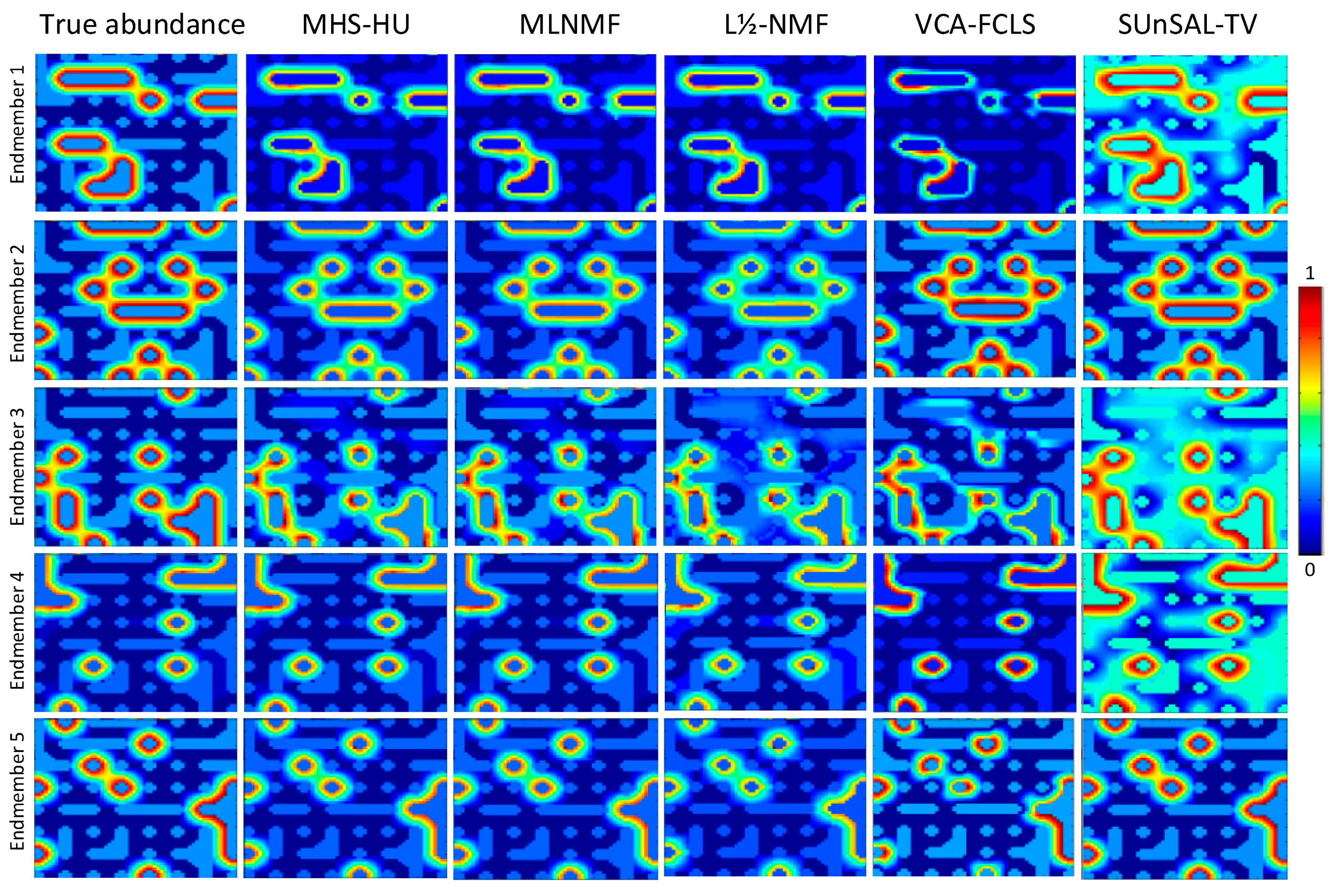
Figure 5.
Abundance maps estimated by the different methods.
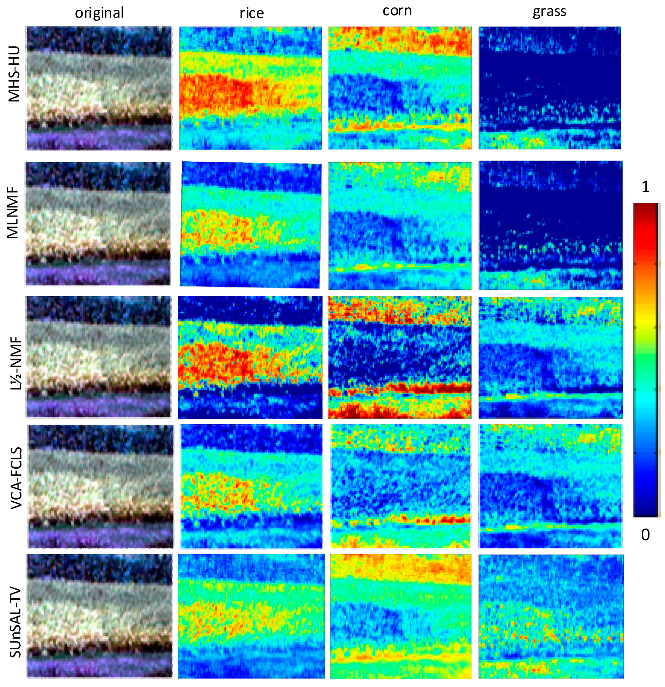
Figure 6.
Fractional abundance maps estimated for the URBAN images.


Table 1.
Comparison of MSEa and RMSE on simulated data.
| Accuracy (10−4) | MHS-HU | MLNMF | VCA-FCLS | L1/2-NMF | SUnSAL-TV |
|---|---|---|---|---|---|
| MSEa | 1.073 | 1.093 | 2.178 | 1.102 | 3.274 |
| RMSE | 1.667 | 1.679 | 3.152 | 1.738 | 33 |
Table 2.
Execution time of the unmixing algorithms on experimental data.
| MHS-HU | SUnSAL-TV | |
|---|---|---|
| simulated data | 10.62s | 88.93s |
Table 3.
Comparison of MSEa, RMSE and rmsSAD accuracy with various scale.
| Value | 2 | 4 | 5 | 6 | 8 |
|---|---|---|---|---|---|
| MSEa (10−4) | 1.0786 | 1.0284 | 1.0244 | 1.0223 | 1.0227 |
| RMSE (10−4) | 1.8750 | 1.8367 | 1.8376 | 1.8431 | 1.8277 |
| rmsSAD | 0.0736 | 0.0683 | 0.0647 | 0.0672 | 0.0676 |
Table 4.
Comparison of MSEa, RMSE and rmsSAD accuracy with various .
| 0 | 0.01 | 0.05 | 0.1 | 0.2 | 0.4 | 0.5 | 0.8 | 1 | 2 | |
|---|---|---|---|---|---|---|---|---|---|---|
| MSEa (10−4) | 1.1177 | 1.1197 | 1.1972 | 1.0943 | 1.0742 | 1.0892 | 1.1100 | 1.2264 | 1.3239 | 1.8116 |
| RMSE (10−4) | 1.7948 | 1.7544 | 1.7447 | 1.7534 | 1.7201 | 1.9674 | 2.2948 | 2.7408 | 3.4200 | 5.5022 |
| rmsSAD | 0.0389 | 0.0374 | 0.0385 | 0.0384 | 0.0387 | 0.0428 | 0.0457 | 0.0555 | 0.0621 | 0.0898 |
Table 5.
Comparison of rsmSAD and RMSE on real data.
| Accuracy | MHS-HU | MLNMF | VCA-FCLS | L1/2-NMF | SUnSAL-TV |
|---|---|---|---|---|---|
| rmsSAD | 0.1940 | 0.2329 | 0.2856 | 0.2415 | X |
| RMSE | 0.0063 | 0.0064 | 0.0114 | 0.0088 | 0.0071 |
Table 6.
Comparison of rmsSAD and RMSE on data with various scale.
| Window Scale | 1 | 3 | 5 | 7 |
|---|---|---|---|---|
| rmsSAD | 0.2079 | 0.1953 | 0.1915 | 0.1917 |
| RMSE | 0.0089 | 0.0064 | 0.0061 | 0.0071 |
Table 7.
Comparison of SAD on Urban data by MHS-HU, MLNMF, L1/2-NMF and VCA-FCLS.
| SAD | MHS-HU | MLNMF | L1/2-NMF | VCA-FCLS |
|---|---|---|---|---|
| Asphalt | 0.1745 | 0.1692 | 0.2027 | 0.1978 |
| Grass | 0.0896 | 0.0890 | 0.2857 | 0.3667 |
| Tree | 0.1682 | 0.1636 | 0.1897 | 0.2155 |
| Roof | 0.1493 | 0.1569 | 0.4611 | 0.4636 |
| shadow | 0.3289 | 0.3489 | 0.4238 | 0.3881 |
| mean | 0.1821 | 0.1855 | 0.3439 | 0.3263 |
Table 8.
Comparison of RMSE on Urban data by MHS-HU, MLNMF, L1/2-NMF and VCA-FCLS.
| RMSE | MHS-HU | MLNMF | L1/2-NMF | VCA-FCLS |
|---|---|---|---|---|
| mean | 0.0195 | 0.0198 | 0.03753 | 0.02102 |
Table 9.
Comparison of rmsSAD and RMSE on Urban data with various scales.
| Window Scale | 1 | 3 | 5 | 7 |
|---|---|---|---|---|
| rmsSAD | 0.2398 | 0.2455 | 0.1821 | 0.2424 |
| RMSE | 0.0211 | 0.0185 | 0.0189 | 0.0198 |
© 2019 by the authors. Licensee MDPI, Basel, Switzerland. This article is an open access article distributed under the terms and conditions of the Creative Commons Attribution (CC BY) license (http://creativecommons.org/licenses/by/4.0/).
Share and Cite
MDPI and ACS Style
Zou, J.; Lan, J. A Multiscale Hierarchical Model for Sparse Hyperspectral Unmixing. Remote Sens. 2019, 11, 500. https://0-doi-org.brum.beds.ac.uk/10.3390/rs11050500
AMA Style
Zou J, Lan J. A Multiscale Hierarchical Model for Sparse Hyperspectral Unmixing. Remote Sensing. 2019; 11(5):500. https://0-doi-org.brum.beds.ac.uk/10.3390/rs11050500
Chicago/Turabian StyleZou, Jinlin, and Jinhui Lan. 2019. "A Multiscale Hierarchical Model for Sparse Hyperspectral Unmixing" Remote Sensing 11, no. 5: 500. https://0-doi-org.brum.beds.ac.uk/10.3390/rs11050500
Note that from the first issue of 2016, this journal uses article numbers instead of page numbers. See further details here.