Feature Comparison and Optimization for 30-M Winter Wheat Mapping Based on Landsat-8 and Sentinel-2 Data Using Random Forest Algorithm

 , , and
Abstract
:1. Introduction
2. Materials and Methods
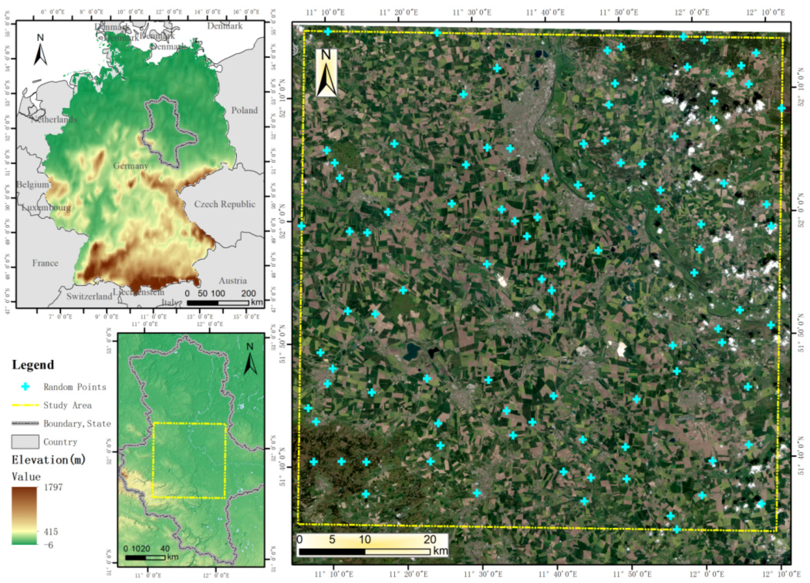
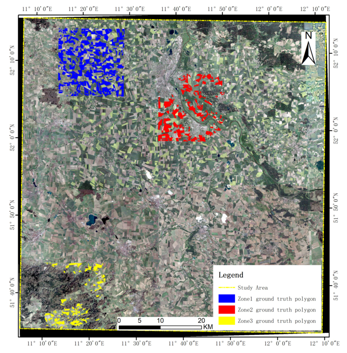
2.1. Study Area
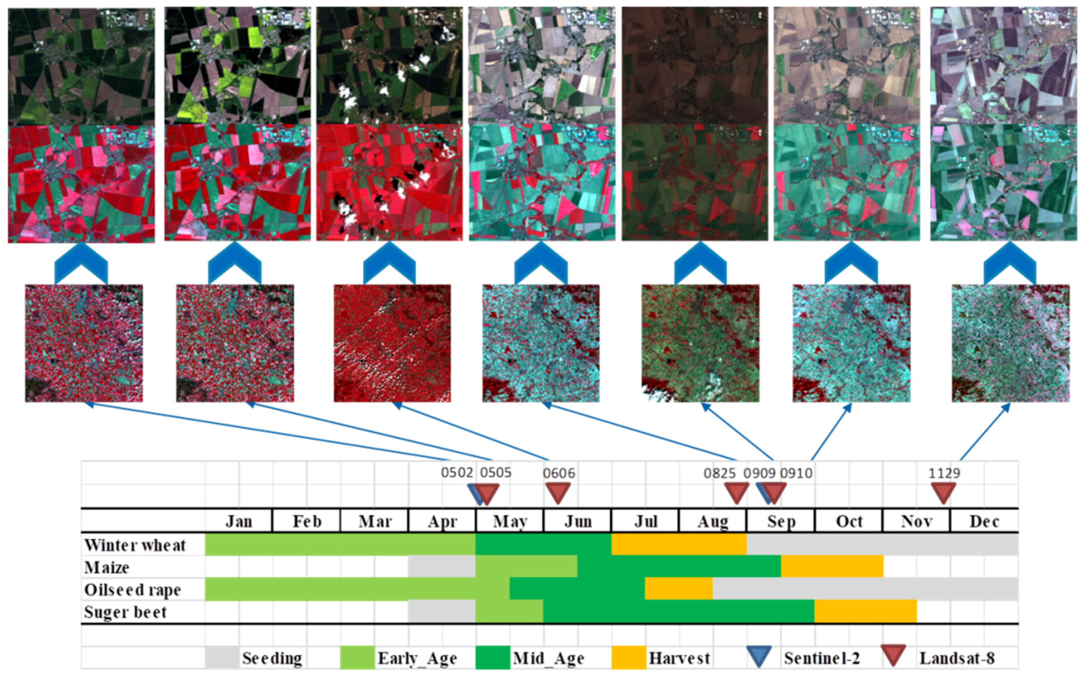
2.2. Satellite Imagery
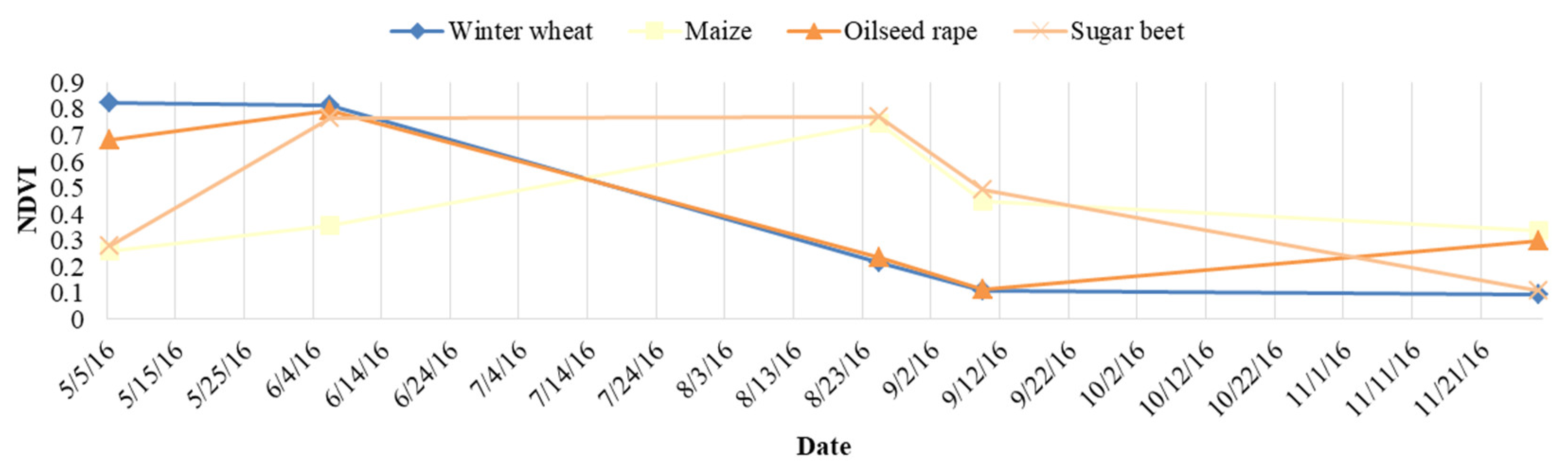
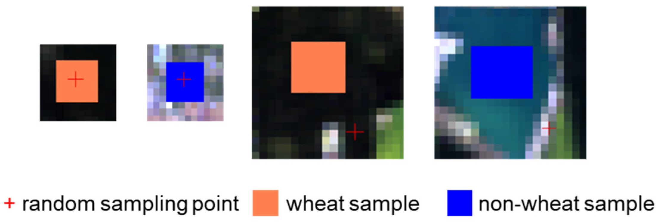
2.3. Reference Data
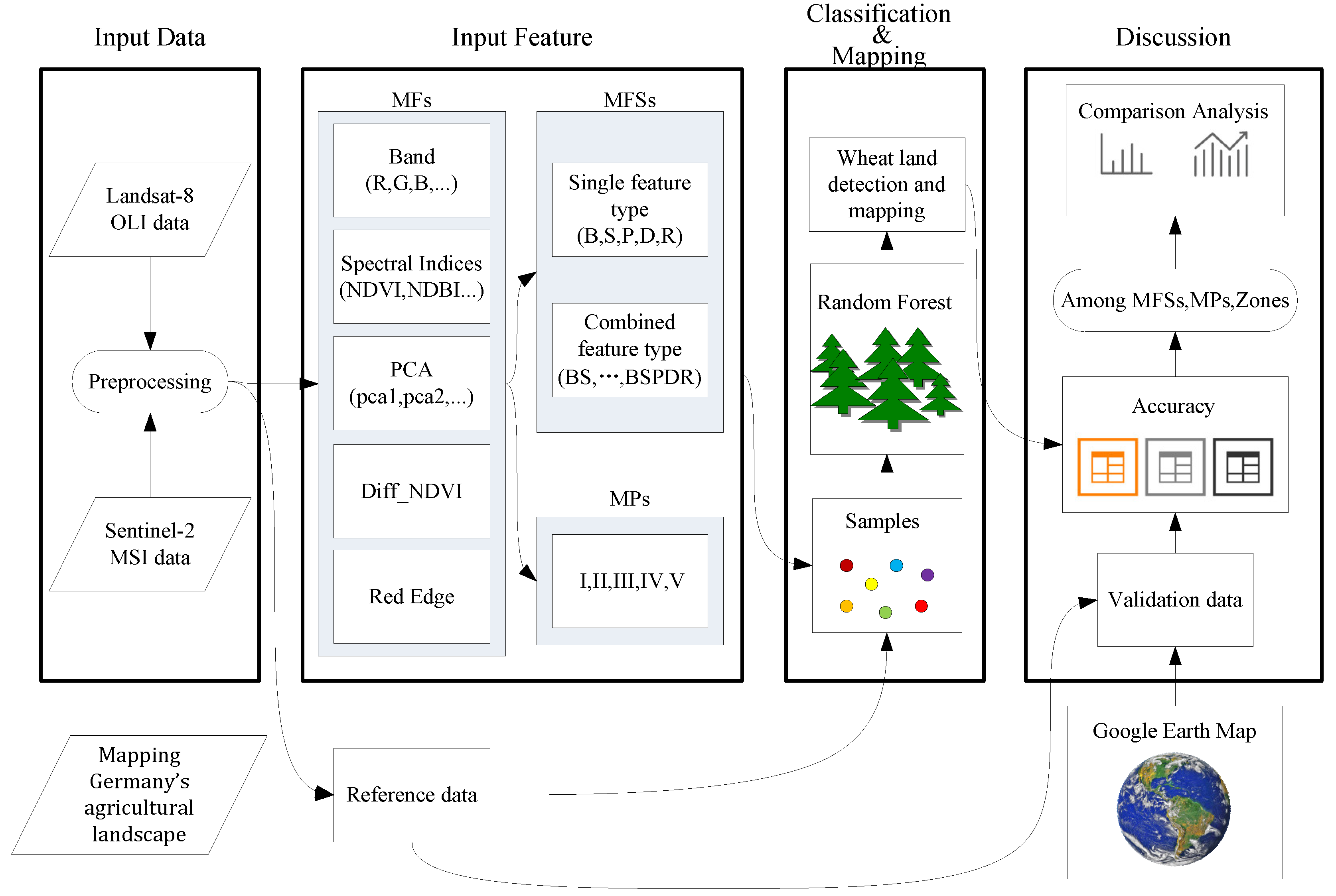
2.4. Methods
2.4.1. Random Forest Algorithm
2.4.2. Multi-Input Features
3. Results
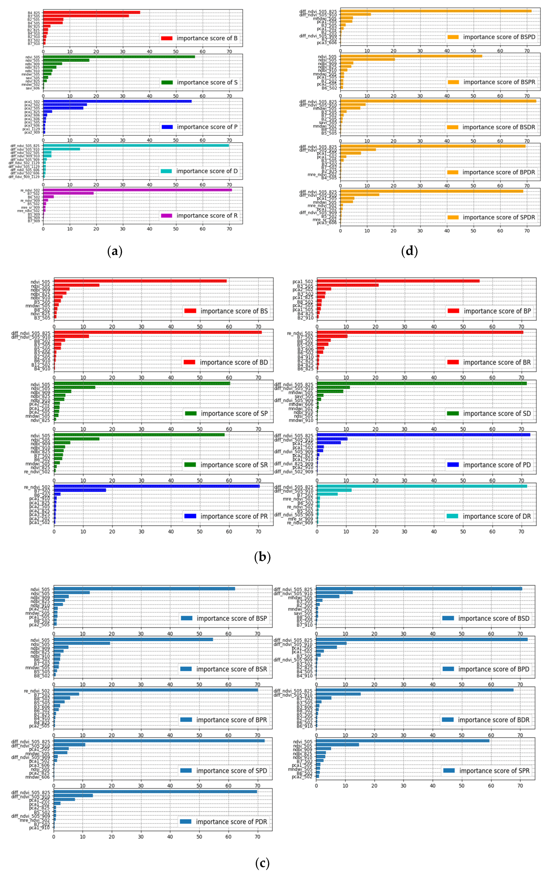
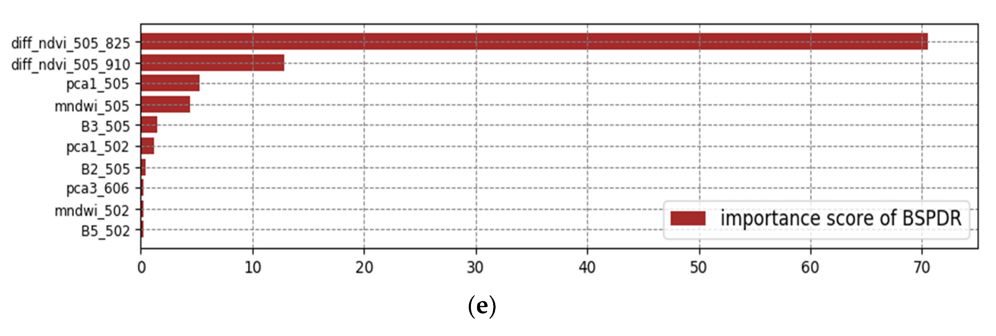
3.1. Key Predictor Variables in MFs
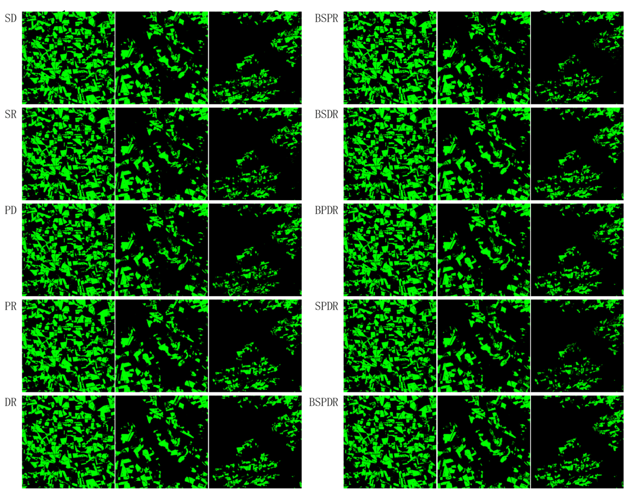
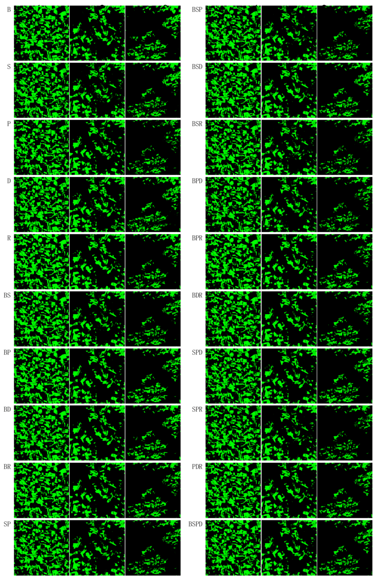
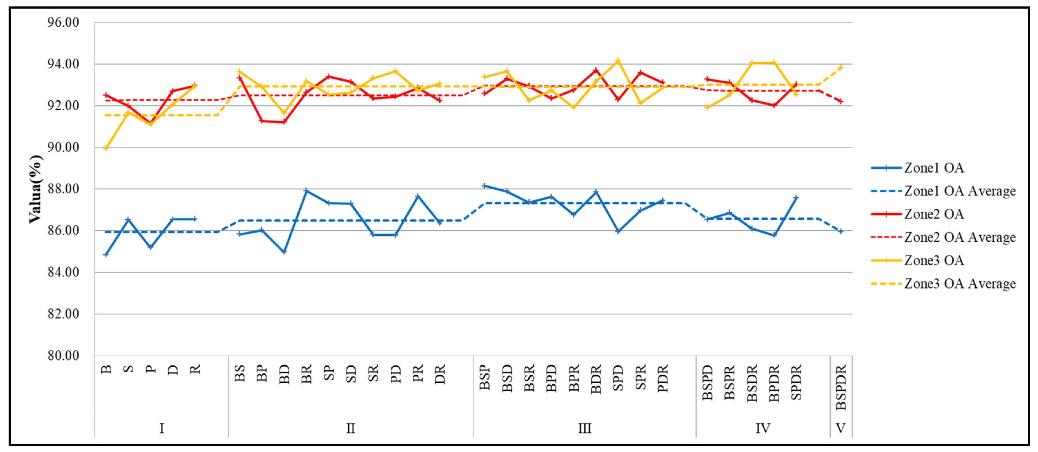
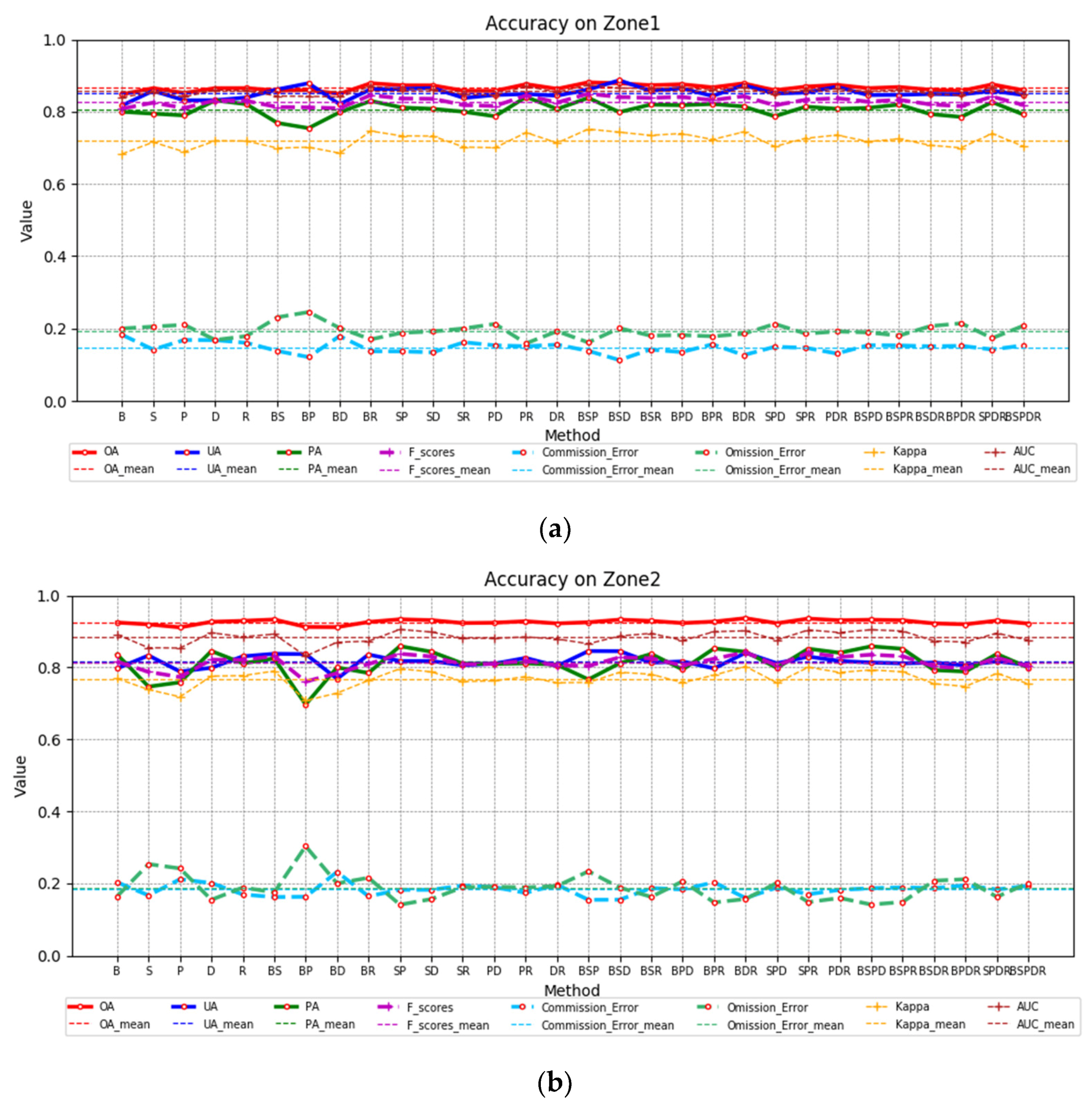
3.2. Mapping Accuracy under 30 MFSs and Five MPs in Three Zones
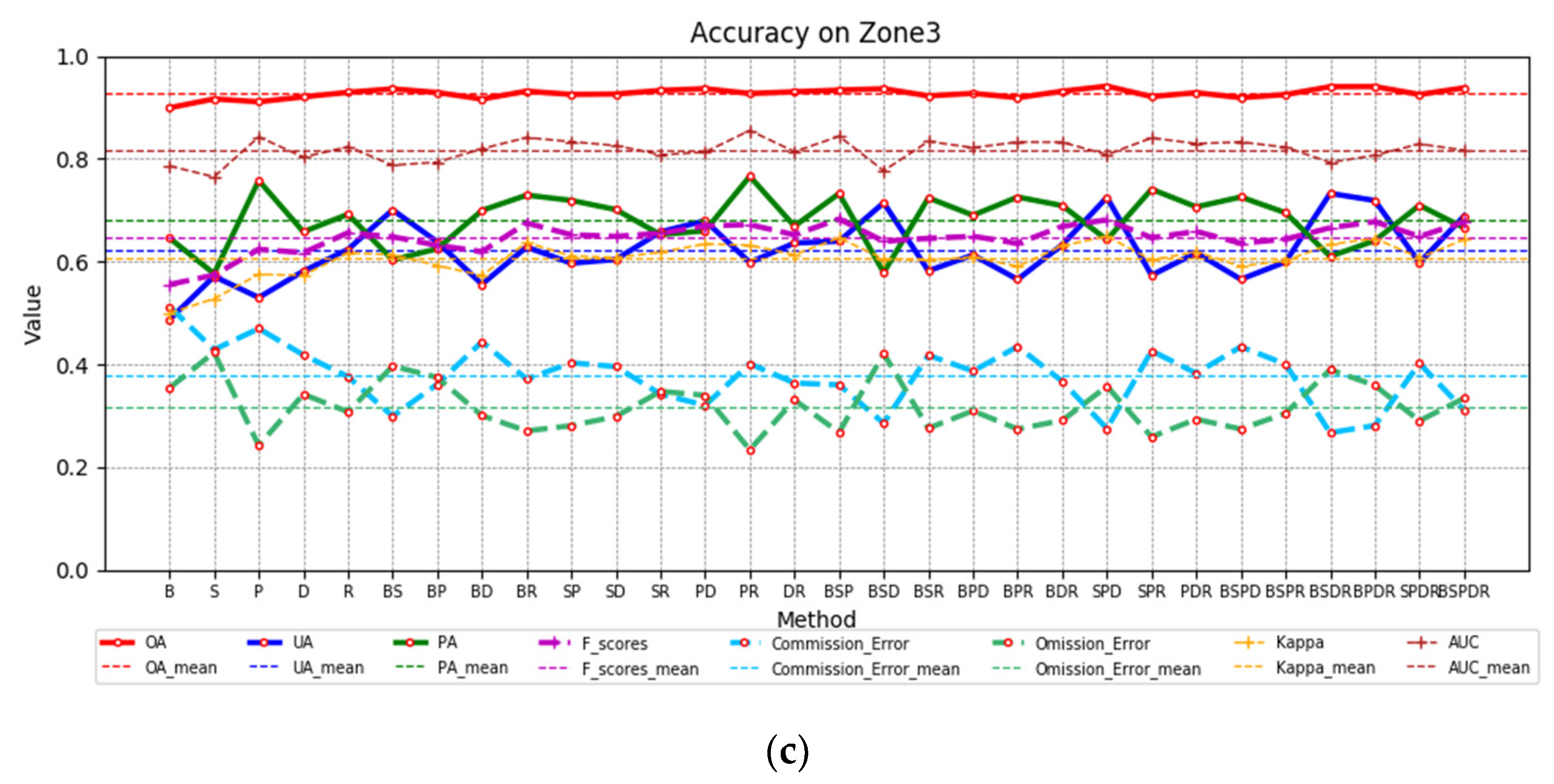
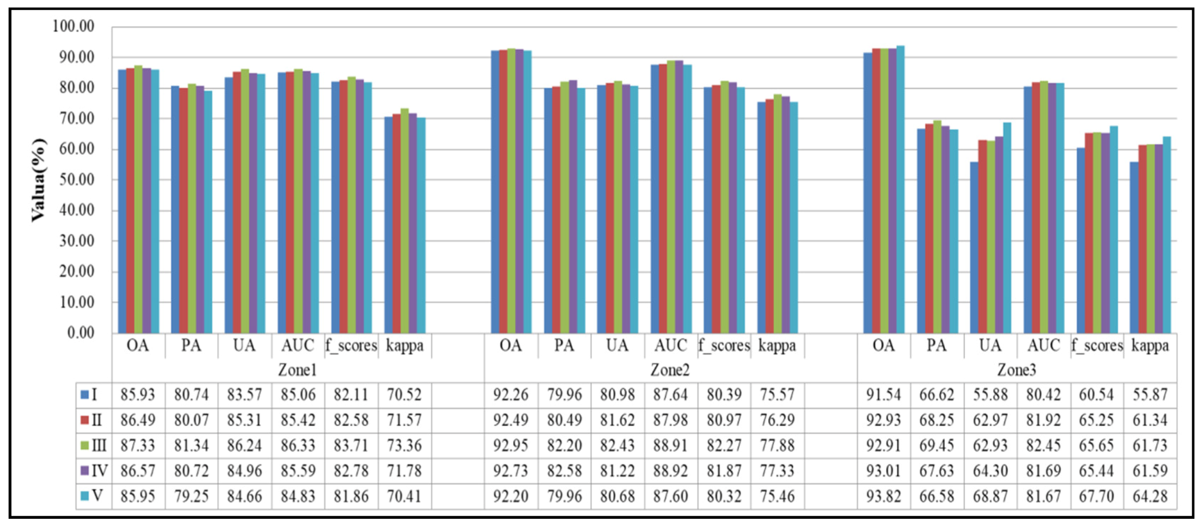
3.3. Accuracy Performance in Three Zones with Multiple Geographical Land Surfaces
4. Discussion
4.1. Optimum Season Selection for MFs
4.2. Optimal MP Selection from MFSs
4.3. Factors Affecting Accuracy in Three Zones
4.4. Prospects of Object-Based Approaches Compared to Pixel-Based Approaches
4.5. Advantages and Limitations of Approach in This Article
5. Conclusions
Author Contributions
Funding
Acknowledgments
Conflicts of Interest
References
- Intergovernmental Panel on Climate Change (IPCC). Climate Change 2014: Synthesis Report. Contribution of Working Groups I, II and III to the Fifth Assessment Report of the Intergovernmental Panel on Climate Change; IPCC: Geneva, Switzerland, 2014; p. 151. [Google Scholar]
- Teluguntla, P.; Thenkabail, P.S.; Xiong, J.; Gumma, M.K.; Congalton, R.G.; Oliphant, A.J.; Sankey, T.; Poehnelt, J.; Yadav, K.; Massey, R.; et al. NASA Making Earth System Data Records for Use in Research Environments (MEaSUREs) Global Food Security-support Analysis Data (GFSAD) @ 30-m for Australia, New Zealand, China, and Mongolia: Cropland Extent Product (GFSAD30AUNZCNMOCE); USGS, EROS, NASA EOSDIS Land Processes DAAC: Sioux Falls, SD, USA, 2017.
- Gumma, M.K.; Thenkabail, P.S.; Teluguntla, P.; Oliphant, A.J.; Xiong, J.; Congalton, R.G.; Yadav, K.; Phalke, A.; Smith, C. NASA Making Earth System Data Records for Use in Research Environments (MEaSUREs) Global Food Security-support Analysis Data (GFSAD) @ 30-m for South Asia, Afghanistan and Iran: Cropland Extent Product (GFSAD30SAAFGIRCE); USGS, EROS, NASA EOSDIS Land Processes DAAC: Sioux Falls, SD, USA, 2017.
- Xiong, J.; Thenkabail, P.S.; Gumma, M.K.; Teluguntla, P.; Poehnelt, J.; Congalton, R.G.; Yadav, K.; Thau, D. Automated cropland mapping of continental Africa using Google Earth Engine cloud computing. ISPRS J. Photogramm. Remote Sens. 2017, 126, 225–244. [Google Scholar] [CrossRef]
- Teluguntla, P.; Thenkabail, P.S.; Xiong, J.; Gumma, M.K.; Congalton, R.G.; Oliphant, A.; Poehnelt, J.; Yadav, K.; Rao, M.; Massey, R. Spectral matching techniques (SMTs) and automated cropland classification algorithms (ACCAs) for mapping croplands of Australia using MODIS 250-m time-series (2000–2015) data. Int. J. Digit. Earth 2017, 10, 944–977. [Google Scholar] [CrossRef]
- Xiong, J.; Thenkabail, P.; Tilton, J.; Gumma, M.; Teluguntla, P.; Oliphant, A.; Congalton, R.; Yadav, K.; Gorelick, N. Nominal 30-m Cropland Extent Map of Continental Africa by Integrating Pixel-Based and Object-Based Algorithms Using Sentinel-2 and Landsat-8 Data on Google Earth Engine. Remote Sens. 2017, 9, 1065. [Google Scholar] [CrossRef]
- Song, X.-P.; Potapov, P.V.; Krylov, A.; King, L.; Di Bella, C.M.; Hudson, A.; Khan, A.; Adusei, B.; Stehman, S.V.; Hansen, M.C. National-scale soybean mapping and area estimation in the United States using medium resolution satellite imagery and field survey. Remote Sens. Environ. 2017, 190, 383–395. [Google Scholar] [CrossRef]
- Huang, Y.; Chen, Z.; Yu, T.; Huang, X.; Gu, X. Agricultural remote sensing big data: Management and applications. J. Integr. Agric. 2018, 17, 1915–1931. [Google Scholar] [CrossRef]
- Zhu, J.; Shi, Q.; Chen, F.; Shi, X.; Do, Z.; Qin, Q. Research status and development trends of remote sensing big data. J. Iamge Graph 2016, 21, 1425–1439. [Google Scholar] [CrossRef]
- Waldner, F.; Lambert, M.-J.; Li, W.; Weiss, M.; Demarez, V.; Morin, D.; Marais-Sicre, C.; Hagolle, O.; Baret, F.; Defourny, P. Land Cover and Crop Type Classification along the Season Based on Biophysical Variables Retrieved from Multi-Sensor High-Resolution Time Series. Remote Sens. 2015, 7, 10400–10424. [Google Scholar] [CrossRef]
- Rodríguez-Galiano, V.F.; Abarca-Hernández, F.; Ghimire, B.; Chica-Olmo, M.; Atkinson, P.M.; Jeganathan, C. Incorporating Spatial Variability Measures in Land-cover Classification using Random Forest. Procedia Environ. Sci. 2011, 3, 44–49. [Google Scholar] [CrossRef]
- Rodriguez-Galiano, V.F.; Chica-Olmo, M.; Abarca-Hernandez, F.; Atkinson, P.M.; Jeganathan, C. Random Forest classification of Mediterranean land cover using multi-seasonal imagery and multi-seasonal texture. Remote Sens. Environ. 2012, 121, 93–107. [Google Scholar] [CrossRef]
- Bargiel, D. A new method for crop classification combining time series of radar images and crop phenology information. Remote Sens. Environ. 2017, 198, 369–383. [Google Scholar] [CrossRef]
- Hao, P.; Wang, L.; Niu, Z.; Aablikim, A.; Huang, N.; Xu, S.; Chen, F. The Potential of Time Series Merged from Landsat-5 TM and HJ-1 CCD for Crop Classification: A Case Study for Bole and Manas Counties in Xinjiang, China. Remote Sens. 2014, 6, 7610–7631. [Google Scholar] [CrossRef]
- Yan, D.; de Beurs, K.M. Mapping the distributions of C3 and C4 grasses in the mixed-grass prairies of southwest Oklahoma using the Random Forest classification algorithm. Int. J. Appl. Earth Obs. Geoinf. 2016, 47, 125–138. [Google Scholar] [CrossRef]
- Wang, N.; Li, Q.; Du, X.; Zhang, Y.; Zhao, L.; Wang, H. Identification of main crops based on the univariate feature selection in Subei. J. Remote Sens. 2017, 21, 519–530. [Google Scholar] [CrossRef]
- Teluguntla, P.; Thenkabail, P.S.; Oliphant, A.; Xiong, J.; Gumma, M.K.; Congalton, R.G.; Yadav, K.; Huete, A. A 30-m landsat-derived cropland extent product of Australia and China using random forest machine learning algorithm on Google Earth Engine cloud computing platform. ISPRS J. Photogramm. Remote Sens. 2018, 144, 325–340. [Google Scholar] [CrossRef]
- Pflugmacher, D.; Rabe, A.; Peters, M.; Hostert, P. Mapping pan-European land cover using Landsat spectral-temporal metrics and the European LUCAS survey. Remote Sens. Environ. 2019, 221, 583–595. [Google Scholar] [CrossRef]
- Griffiths, P.; Nendel, C.; Hostert, P. Intra-annual reflectance composites from Sentinel-2 and Landsat for national-scale crop and land cover mapping. Remote Sens. Environ. 2019, 220, 135–151. [Google Scholar] [CrossRef]
- Wu, B.; Zhang, M. Remote sensing: Observations to data products. Acta Geogr. Sin. 2017, 72, 2093–2111. [Google Scholar] [CrossRef]
- Breiman, L. Random Forest. Mach. Learn. 2001, 45, 5–32. [Google Scholar] [CrossRef]
- Hao, P.; Zhan, Y.; Wang, L.; Niu, Z.; Shakir, M. Feature Selection of Time Series MODIS Data for Early Crop Classification Using Random Forest: A Case Study in Kansas, USA. Remote Sens. 2015, 7, 5347–5369. [Google Scholar] [CrossRef]
- Pelletier, C.; Valero, S.; Inglada, J.; Champion, N.; Dedieu, G. Assessing the robustness of Random Forests to map land cover with high resolution satellite image time series over large areas. Remote Sens. Environ. 2016, 187, 156–168. [Google Scholar] [CrossRef]
- Gao, J.; Nuyttens, D.; Lootens, P.; He, Y.; Pieters, J.G. Recognising weeds in a maize crop using a random forest machine-learning algorithm and near-infrared snapshot mosaic hyperspectral imagery. Biosyst. Eng. 2018, 170, 39–50. [Google Scholar] [CrossRef]
- Gislason, P.O.; Benediktsson, J.A.; Sveinsson, J.R. Random Forests for land cover classification. Pattern. Recogn. Lett. 2006, 27, 294–300. [Google Scholar] [CrossRef]
- Jhonnerie, R.; Siregar, V.P.; Nababan, B.; Prasetyo, L.B.; Wouthuyzen, S. Random Forest Classification for Mangrove Land Cover Mapping Using Landsat 5 TM and Alos Palsar Imageries. Procedia Environ. Sci. 2015, 24, 215–221. [Google Scholar] [CrossRef]
- Melville, B.; Lucieer, A.; Aryal, J. Object-based random forest classification of Landsat ETM+ and WorldView2 satellite imagery for mapping lowland native grassland communities in Tasmania, Australia. Int. J. Appl. Earth Obs. Geoinf. 2018, 66, 46–55. [Google Scholar] [CrossRef]
- Rodriguez-Galiano, V.F.; Ghimire, B.; Rogan, J.; Chica-Olmo, M.; Rigol-Sanchez, J.P. An assessment of the effectiveness of a random forest classifier for land-cover classification. ISPRS J. Photogramm. Remote Sens. 2012, 67, 93–104. [Google Scholar] [CrossRef]
- Tatsumi, K.; Yamashiki, Y.; Canales Torres, M.A.; Taipe, C.L.R. Crop classification of upland fields using Random forest of time-series Landsat 7 ETM+ data. Comput. Electron. Agric. 2015, 115, 171–179. [Google Scholar] [CrossRef]
- Huang, H.; Chen, Y.; Clinton, N.; Wang, J.; Wang, X.; Liu, C.; Gong, P.; Yang, J.; Bai, Y.; Zheng, Y.; et al. Mapping major land cover dynamics in Beijing using all Landsat images in Google Earth Engine. Remote Sens. Environ. 2017, 202, 166–176. [Google Scholar] [CrossRef]
- Zurqani, H.A.; Post, C.J.; Mikhailova, E.A.; Schlautman, M.A.; Sharp, J.L. Geospatial analysis of land use change in the Savannah River Basin using Google Earth Engine. Int. J. Appl. Earth Obs. Geoinf. 2018, 69, 175–185. [Google Scholar] [CrossRef]
- Wang, X.; Xiao, X.; Zou, Z.; Chen, B.; Ma, J.; Dong, J.; Doughty, R.B.; Zhong, Q.; Qin, Y.; Dai, S.; et al. Tracking annual changes of coastal tidal flats in China during 1986–2016 through analyses of Landsat images with Google Earth Engine. Remote Sens. Environ. 2018. [Google Scholar] [CrossRef]
- Liu, X.; Hu, G.; Chen, Y.; Li, X.; Xu, X.; Li, S.; Pei, F.; Wang, S. High-resolution multi-temporal mapping of global urban land using Landsat images based on the Google Earth Engine Platform. Remote Sens. Environ. 2018, 209, 227–239. [Google Scholar] [CrossRef]
- Li, H.; Wan, W.; Fang, Y.; Zhu, S.; Chen, X.; Liu, B.; Hong, Y. A Google Earth Engine-enabled software for efficiently generating high-quality user-ready Landsat mosaic images. Environ. Model. Softw. 2019, 112, 16–22. [Google Scholar] [CrossRef]
- Yin, H.; Prishchepov, A.V.; Kuemmerle, T.; Bleyhl, B.; Buchner, J.; Radeloff, V.C. Mapping agricultural land abandonment from spatial and temporal segmentation of Landsat time series. Remote Sens. Environ. 2018, 210, 12–24. [Google Scholar] [CrossRef]
- Kussul, N.; Lemoine, G.; Gallego, F.J.; Skakun, S.V.; Lavreniuk, M.; Shelestov, A.Y. Parcel-Based Crop Classification in Ukraine Using Landsat-8 Data and Sentinel-1A Data. IEEE J. Sel. Top. Appl. Earth Obs. Remote Sens. 2016, 9, 2500–2508. [Google Scholar] [CrossRef]
- Tian, H.; Wu, M.; Wang, L.; Niu, Z. Mapping Early, Middle and Late Rice Extent Using Sentinel-1A and Landsat-8 Data in the Poyang Lake Plain, China. Sensors 2018, 18, 185. [Google Scholar] [CrossRef] [PubMed]
- Belgiu, M.; Csillik, O. Sentinel-2 cropland mapping using pixel-based and object-based timeweighted dynamic time warping analysis. Remote Sens. Environ. 2018, 204, 209–523. [Google Scholar] [CrossRef]
- Frampton, W.J.; Dash, J.; Watmough, G.; Milton, E.J. Evaluating the capabilities of Sentinel-2 for quantitative estimation of biophysical variables in vegetation. ISPRS J. Photogramm. Remote Sens. 2013, 82, 83–92. [Google Scholar] [CrossRef]
- Vuolo, F.; Neuwirth, M.; Immitzer, M.; Atzberger, C.; Ng, W.-T. How much does multi-temporal Sentinel-2 data improve crop type classification? Int. J. Appl. Earth Obs. Geoinf. 2018, 72, 122–130. [Google Scholar] [CrossRef]
- Lessio, A.; Fissore, V.; Borgogno-Mondino, E. Preliminary Tests and Results Concerning Integration of Sentinel-2 and Landsat-8 OLI for Crop Monitoring. J. Imaging 2017, 3, 49. [Google Scholar] [CrossRef]
- Li, Z.; Zhang, H.K.; Roy, D.P.; Yan, L.; Huang, H.; Li, J. Landsat 15-m Panchromatic-Assisted Downscaling (LPAD) of the 30-m Reflective Wavelength Bands to Sentinel-2 20-m Resolution. Remote Sens. 2017, 9, 755. [Google Scholar] [CrossRef]
- Skakun, S.; Vermote, E.; Roger, J.C.; Franch, B. Combined use of Landsat-8 and Sentinel-2A images for winter crop mapping and winter wheat yield assessment at regional scale. Aims Geosci. 2017, 3, 163–186. [Google Scholar] [CrossRef]
- Clark, M.L. Comparison of simulated hyperspectral HyspIRI and multispectral Landsat 8 and Sentinel-2 imagery for multi-seasonal, regional land-cover mapping. Remote Sens. Environ. 2017, 200, 311–325. [Google Scholar] [CrossRef]
- Novelli, A.; Aguilar, M.; Nemmaoui, A.; Aguilar, F.; Tarantino, E. Performance evaluation of object based greenhouse detection from Sentinel-2 MSI and Landsat 8 OLI data: A case study from Almería (Spain). Int. J. Appl. Earth Obs. Geoinf. 2016, 52, 403–411. [Google Scholar] [CrossRef]
- Shoko, C.; Mutanga, O. Examining the strength of the newly-launched Sentinel 2 MSI sensor in detecting and discriminating subtle differences between C3 and C4 grass species. ISPRS J. Photogramm. Remote Sens. 2017, 129, 32–40. [Google Scholar] [CrossRef]
- Vuolo, F.; Żółtak, M.; Pipitone, C.; Zappa, L.; Wenng, H.; Immitzer, M.; Weiss, M.; Baret, F.; Atzberger, C. Data Service Platform for Sentinel-2 Surface Reflectance and Value-Added Products: System Use and Examples. Remote Sens. 2016, 8, 938. [Google Scholar] [CrossRef]
- Chastain, R.; Housman, I.; Goldstein, J.; Finco, M.; Tenneson, K. Empirical cross sensor comparison of Sentinel-2A and 2B MSI, Landsat-8 OLI, and Landsat-7 ETM+ top of atmosphere spectral characteristics over the conterminous United States. Remote Sens. Environ. 2019, 221, 274–285. [Google Scholar] [CrossRef]
- Thenkabail, P.S.; Biradar, C.M.; Turral, H.; Noojipady, P.; Li, Y.J.; Vithanage, J.; Dheeravath, V.; Velpuri, M.; Schull, M.; Cai, X.L.; Dutta, R. An Irrigated Area Map of the World (1999) derived from Remote Sensing. IWMI Res. Rep. 2006, 105. [Google Scholar] [CrossRef]
- Biradar, C.M.; Thenkabail, P.S.; Noojipady, P.; Li, Y.; Dheeravath, V.; Turral, H.; Velpuri, M.; Gumma, M.K.; Gangalakunta, O.R.P.; Cai, X.L.; et al. A global map of rainfed cropland areas (GMRCA) at the end of last millennium using remote sensing. Int. J. Appl. Earth Obs. Geoinf. 2009, 11, 114–129. [Google Scholar] [CrossRef]
- Velpuri, N.M.; Thenkabail, P.S.; Gumma, M.K.; Biradar, C.; Dheeravath, V.; Noojipady, P.; Yuanjie, L. Influence of resolution in irrigated area mapping and area estimation.pdf. Photogramm. Eng. Remote Sens. 2009, 75, 1383–1396. [Google Scholar] [CrossRef]
- Dheeravath, V.; Thenkabail, P.S.; Chandrakantha, G.; Noojipady, P.; Reddy, G.P.O.; Biradar, C.M.; Gumma, M.K.; Velpuri, M. Irrigated areas of India derived using MODIS 500 m time series for the years 2001–2003. ISPRS J. Photogramm. Remote Sens. 2010, 65, 42–59. [Google Scholar] [CrossRef]
- Radoux, J.; Chomé, G.; Jacques, D.; Waldner, F.; Bellemans, N.; Matton, N.; Lamarche, C.; d’Andrimont, R.; Defourny, P. Sentinel-2’s Potential for Sub-Pixel Landscape Feature Detection. Remote Sens. 2016, 8, 488. [Google Scholar] [CrossRef]
- Meier, U. Growth Stages of Mono-and Dicotyledonous Plants—BBCH Monograph; Federal Biological Research Centre for Agriculture and Forestry: Bonn, Germany, 2001. [Google Scholar]
- Breiman, L. Bagging Predictors. Mach. Learn. 1996, 26, 123–140. [Google Scholar] [CrossRef]
- Dietterich, T.G. An experimental comparison of three methods for constructing ensembles of decision trees_Bagging, boosting and randomization. Mach. Learn. 2000, 40, 139–157. [Google Scholar] [CrossRef]
- Congalton, R.G. A Review of Assessing the Accuracy of Classifications of Remotely Sensed Data. Remote Sens. Environ. 1991, 37, 35–46. [Google Scholar] [CrossRef]
- Potere, D. Horizontal Positional Accuracy of Google Earth’s High-Resolution Imagery Archive. Sensors (Basel) 2008, 8, 7973–7981. [Google Scholar] [CrossRef]
- Jaafari, S.; Nazarisamani, A. Comparison between Land Use/Land Cover Mapping Through Landsat and Google Earth Imagery. Am. Eurasian J. Agric. Environ. Sci. 2013, 13, 763–768. [Google Scholar] [CrossRef]
- Dorais, A.; Cardille, J. Strategies for Incorporating High-Resolution Google Earth Databases to Guide and Validate Classifications: Understanding Deforestation in Borneo. Remote Sens. 2011, 3, 1157–1176. [Google Scholar] [CrossRef]
- Cha, S.-Y.; Park, C.-H. The Utilization of Google Earth Images as Reference Data for The Multitemporal Land Cover Classification with MODIS Data of North Korea. Korean J. Remote Sens. 2007, 23, 483–491. [Google Scholar]
- Goudarzi, M.A.; Landry, R., Jr. Assessing horizontal positional accuracy of Google Earth imagery in the city of Montreal, Canada. Geod. Cartogr. 2017, 43, 56–65. [Google Scholar] [CrossRef]
- Story, M.; Congalton, R.G. Accuracy Assessment_A User’s Perspective. Photogramm. Eng. Remote Sens. 1986, 52, 397–399. [Google Scholar]
- Cohen, J. A coefficient of agreement for nominal scales. Educ. Psychol. Meas 1960, 1. [Google Scholar] [CrossRef]
- Rouse, J.W., Jr.; Haas, R.H.; Well, J.A.; Deering, D.W. Monitoring Vegetation Systems in the Great Plains with Erts. In Third Earth Resources Technology Satellite-1 Symposium—Volume I: Technical Presentations; NASA: Washington, DC, USA, 1974; pp. 309–371. [Google Scholar]
- Huete, A.; Didan, K.; Miura, T.; Rodriguez, E.P.; Gao, X.; Ferreira, L.G. Overview of the Radiometric and Biophysical Performance of the MODIS Vegetation Indices. Remote Sens. Environ. 2002, 83, 195–213. [Google Scholar] [CrossRef]
- Kauth, R.J.; Thomas, G.S. The Tasselled Cap—A Graphic Description of the Spectral-Temporal Development of Agricultural Crops as Seen by Landsat; LARS Symposia Paper 159; Purdue University: West Lafayette, IN, USA, 1976; pp. 40–51. [Google Scholar]
- Sripada, R.P.; Heiniger, R.W.; White, J.G.; Meijer, A.D. Aerial Color Infrared Photography for Determining Early In-season Nitrogen Requirements in Corn. Remote Sens. 2006, 98, 968–977. [Google Scholar] [CrossRef]
- Boegha, E.; Soegaard, H.; Broge, N.; Hasager, C.B.; Jensen, N.O.; Schelde, K.; Thomsen, A. Airborne Multi-spectral Data for Quantifying Leaf Area Index-Nitrogen Concentration and Photosynthetic Efficiency in Agriculture. Remote Sens. Environ. 2002, 81, 179–193. [Google Scholar] [CrossRef]
- Zha, Y.; Gao, J.; Ni, S. Use of Normalized Difference Built-Up Index in Automatically Mapping Urban Areas from TM Imagery. Int. J. Remote Sens. 2003, 24, 583–594. [Google Scholar] [CrossRef]
- Hall, D.K.; Riggs, G.A.; Salomonson, V.V. Development of Methods for Mapping Global Snow Cover Using Moderate Resolution Imaging Spectroradiometer Data. Remote Sens. Environ. 1995, 54, 127–140. [Google Scholar] [CrossRef]
- McFeeters, S.K. The use of the Normalized Difference Water Index (NDWI) in the delineation of open water features. Int. J. Remote Sens. 2007, 17, 1425–1432. [Google Scholar] [CrossRef]
- Xu, H. Modification of normalised difference water index (NDWI) to enhance open water features in remotely sensed imagery. Int. J. Remote Sens. 2006, 27, 3025–3033. [Google Scholar] [CrossRef]
- Huete, A.R. A soil-adjusted vegetation index (SAVI). Remote Sens. Environ. 1988, 25, 295–309. [Google Scholar] [CrossRef]
- Lobell, D.B.; Asner, G.P. Hyperion Studies of Crop Stress in Mexico. In Proceedings of the 12th Annual Jpl Airborne Earth Sci. Workshop, Pasadena, CA, USA, 24–28 February 2003; pp. 1–6. [Google Scholar]
- Gerald, S.B.; George, R.M. Measuring the Color of Growing Turf with a Reflectance Spectrophotometer. Agron. J. 1968, 60, 640–643. [Google Scholar]
- Haralick, R.M.; Shanmugam, K.; Dinstein, I.H. Textural Features for Image Classification. IEEE Trans. Syst. Man Cybern. 1973, SMC-3, 610–621. [Google Scholar] [CrossRef]
- Jiang, Q.; Liu, H. Extracting TM Image Information Using Texture Analysis. J. Remote Sens. 2004, 8, 458–464. [Google Scholar]
- Fernández-Manso, A.; Fernández-Manso, O.; Quintano, C. SENTINEL-2A red-edge spectral indices suitability for discriminating burn severity. Int. J. Appl. Earth Obs. Geoinf. 2016, 50, 170–175. [Google Scholar] [CrossRef]
- Dube, T.; Mutanga, O.; Sibanda, M.; Shoko, C.; Chemura, A. Evaluating the influence of the Red Edge band from RapidEye sensor in quantify. Phys. Chem. Earth 2017, 100, 73–80. [Google Scholar] [CrossRef]
- Li, L.; Ren, T.; Ma, Y.; Wei, Q.; Wang, S.; Li, X.; Cong, R.; Liu, S.; Lu, J. Evaluating chlorophyll density in winter oilseed rape ( Brassica napus L.) using canopy hyperspectral red-edge parameters. Comput. Electron. Agric. 2016, 126, 21–31. [Google Scholar] [CrossRef]
- Guo, B.-B.; Qi, S.-L.; Heng, Y.-R.; Duan, J.-Z.; Zhang, H.-Y.; Wu, Y.-P.; Feng, W.; Xie, Y.-X.; Zhu, Y.-J. Remotely assessing leaf N uptake in winter wheat based on canopy hyperspectral red-edge absorption. Eur. J. Agron. 2017, 82, 113–124. [Google Scholar] [CrossRef]
- Nitze, I.; Barrett, B.; Cawkwell, F. Temporal optimisation of image acquisition for land cover classification with Random Forest and MODIS time-series. Int. J. Appl. Earth Obs. Geoinf. 2015, 34, 136–146. [Google Scholar] [CrossRef]
- Smith, V.; Portillo-Quintero, C.; Sanchez-Azofeifa, A.; Hernandez-Stefanoni, J.L. Assessing the accuracy of detected breaks in Landsat time series as predictors of small scale deforestation in tropical dry forests of Mexico and Costa Rica. Remote Sens. Environ. 2019, 221, 707–721. [Google Scholar] [CrossRef]
- Zhang, Y.; Ling, F.; Foody, G.M.; Ge, Y.; Boyd, D.S.; Li, X.; Du, Y.; Atkinson, P.M. Mapping annual forest cover by fusing PALSAR/PALSAR-2 and MODIS NDVI during 2007–2016. Remote Sens. Environ. 2019, 224, 74–91. [Google Scholar] [CrossRef]
- Schultz, B.; Immitzer, M.; Formaggio, A.; Sanches, I.; Luiz, A.; Atzberger, C. Self-Guided Segmentation and Classification of Multi-Temporal Landsat 8 Images for Crop Type Mapping in Southeastern Brazil. Remote Sens. 2015, 7, 14482–14508. [Google Scholar] [CrossRef]


| Institution | Products | Scale | Resolution |
|---|---|---|---|
| European Space Agency (ESA) (30 m Sentinel-2 and Landsat-8) |
| Regional | 30 m |
| McGill University |
| Global | 10 km |
| International Water Management Institute (IWMI) |
| Global | 10 km |
| Global | 10 km | |
| Regional | 500 m | |
| Regional | 30 m | |
| United States Geological Survey (USGS) (GFSAD30 and Landsat) |
| Global | 30 m |
| Date | 0502 | 0505 | 0606 | 0825 | 0909 | 0910 | 1129 | |
|---|---|---|---|---|---|---|---|---|
| Features | ||||||||
| Bands | 2 3 4 8 11 12 | 2 3 4 5 6 7 | 2 3 4 5 6 7 | 2 3 4 5 6 7 | 2 3 4 8 11 12 | 2 3 4 5 6 7 | 2 3 4 5 6 7 | |
| Spectral Indices | ndvi_502 | ndvi_505 | ndvi_606 | nfvi_825 | ndvi_909 | ndvi_910 | ndvi_1129 | |
| ndbi_502 | ndbi_825 | ndbi_606 | ndbi_825 | ndbi_909 | ndbi_910 | ndbi_1129 | ||
| ndsi_502 | ndsi_505 | ndsi_606 | ndsi_825 | ndsi_909 | ndsi_910 | ndsi_1129 | ||
| mndwi_502 | mndwi_505 | mdnwi_606 | mndwi_825 | mndwi_909 | mndwi_910 | mndwi_1129 | ||
| savi_502 | savi_505 | savi_606 | savi_825 | savi_909 | savi_910 | savi_1129 | ||
| Principal Component Analysis (PCA) | pca1_502 | pca1_505 | pca1_606 | pca1_825 | pca1_909 | pca1_910 | pca1_1129 | |
| pca2_502 | pca2_505 | pca2_606 | pca2_825 | pca2_909 | pca2_910 | pca2_1129 | ||
| pca3_502 | pca3_505 | pca3_606 | pca3_825 | pca3_909 | pca3_910 | pca3_1129 | ||
| Diff_Ndvi | ndvi_502_505 | ndvi_505_606 | ndvi_606_825 | ndvi_825_909 | ndvi_909_910 | ndvi_910_1129 | ||
| ndvi_502_606 | ndvi_505_825 | ndvi_606_909 | ndvi_825_910 | ndvi_909_910 | ||||
| ndvi_502_825 | ndvi_505_909 | ndvi_606_910 | ndvi_825_1129 | |||||
| ndvi_502_909 | ndvi_505_910 | ndvi_606_1129 | ||||||
| ndvi_502_910 | ndvi_505_1129 | |||||||
| ndvi_502_1129 | ||||||||
| Red_Edge | 5 6 7 | 5 6 7 | ||||||
| mre_ndvi_502 | mre_ndvi_909 | |||||||
| mre_sr_502 | mre_sr_909 | |||||||
| re_ndvi_502 | re_ndvi_909 | |||||||
| Feature | Zone 1 | Zone 2 | Zone 3 | ||||||||||||||||
|---|---|---|---|---|---|---|---|---|---|---|---|---|---|---|---|---|---|---|---|
| OA | PA | UA | AUC | f_Scores | kappa | OA | PA | UA | AUC | f_Scores | kappa | OA | PA | UA | AUC | f_Scores | kappa | ||
| I | B | 84.84 | 79.99 | 81.74 | 0.8403 | 0.8086 | 0.6831 | 92.50 | 83.59 | 79.71 | 0.8915 | 0.8161 | 0.7690 | 89.94 | 64.59 | 48.72 | 0.7863 | 0.5555 | 0.5000 |
| S | 86.52 | 79.47 | 85.80 | 0.8535 | 0.8251 | 0.7157 | 91.98 | 74.66 | 83.33 | 0.8547 | 0.7876 | 0.7384 | 91.67 | 57.66 | 57.13 | 0.7650 | 0.5740 | 0.5278 | |
| P | 85.19 | 78.98 | 83.16 | 0.8415 | 0.8102 | 0.6889 | 91.14 | 75.85 | 78.86 | 0.8540 | 0.7733 | 0.7183 | 91.11 | 75.79 | 53.02 | 0.8428 | 0.6239 | 0.5753 | |
| D | 86.54 | 83.15 | 83.19 | 0.8597 | 0.8317 | 0.7195 | 92.69 | 84.56 | 79.91 | 0.8964 | 0.8217 | 0.7758 | 92.06 | 65.81 | 58.15 | 0.8035 | 0.6174 | 0.5733 | |
| R | 86.55 | 82.09 | 83.95 | 0.8581 | 0.8301 | 0.7189 | 92.96 | 81.15 | 83.08 | 0.8852 | 0.8210 | 0.7772 | 92.94 | 69.22 | 62.38 | 0.8236 | 0.6562 | 0.6170 | |
| Avg | 85.93 | 80.74 | 83.57 | 0.8506 | 0.8211 | 0.7052 | 92.26 | 79.96 | 80.98 | 0.8764 | 0.8039 | 0.7557 | 91.54 | 66.62 | 55.88 | 0.8042 | 0.6054 | 0.5587 | |
| II | BS | 85.83 | 76.89 | 86.20 | 0.8434 | 0.8128 | 0.6993 | 93.34 | 82.50 | 83.79 | 0.8927 | 0.8314 | 0.7899 | 93.63 | 60.33 | 70.08 | 0.7877 | 0.6484 | 0.6136 |
| BP | 86.02 | 75.45 | 87.89 | 0.8426 | 0.8120 | 0.7017 | 91.27 | 69.69 | 83.72 | 0.8316 | 0.7606 | 0.7078 | 92.91 | 62.51 | 63.85 | 0.7935 | 0.6317 | 0.5925 | |
| BD | 84.97 | 79.86 | 82.08 | 0.8412 | 0.8096 | 0.6854 | 91.21 | 80.00 | 76.83 | 0.8700 | 0.7838 | 0.7287 | 91.64 | 69.96 | 55.59 | 0.8197 | 0.6195 | 0.5733 | |
| BR | 87.91 | 82.99 | 86.27 | 0.8709 | 0.8460 | 0.7465 | 92.64 | 78.45 | 83.58 | 0.8731 | 0.8093 | 0.7638 | 93.17 | 72.94 | 62.85 | 0.8414 | 0.6752 | 0.6372 | |
| SP | 87.32 | 81.17 | 86.32 | 0.8629 | 0.8366 | 0.7331 | 93.39 | 85.91 | 81.79 | 0.9058 | 0.8380 | 0.7965 | 92.54 | 71.92 | 59.69 | 0.8334 | 0.6524 | 0.6110 | |
| SD | 87.30 | 80.81 | 86.57 | 0.8622 | 0.8359 | 0.7325 | 93.15 | 84.37 | 81.78 | 0.8985 | 0.8306 | 0.7876 | 92.62 | 70.13 | 60.42 | 0.8259 | 0.6491 | 0.6082 | |
| SR | 85.80 | 79.98 | 83.81 | 0.8483 | 0.8185 | 0.7020 | 92.35 | 81.07 | 80.62 | 0.8811 | 0.8085 | 0.7607 | 93.32 | 65.25 | 65.80 | 0.8079 | 0.6552 | 0.6182 | |
| PD | 85.78 | 78.73 | 84.65 | 0.8461 | 0.8159 | 0.7003 | 92.44 | 80.95 | 81.04 | 0.8812 | 0.8100 | 0.7627 | 93.66 | 66.01 | 67.95 | 0.8133 | 0.6697 | 0.6346 | |
| PR | 87.65 | 84.10 | 84.89 | 0.8706 | 0.8449 | 0.7423 | 92.85 | 81.14 | 82.65 | 0.8845 | 0.8189 | 0.7744 | 92.72 | 76.60 | 59.85 | 0.8553 | 0.6720 | 0.6317 | |
| DR | 86.35 | 80.75 | 84.46 | 0.8542 | 0.8256 | 0.7136 | 92.24 | 80.75 | 80.38 | 0.8793 | 0.8057 | 0.7572 | 93.06 | 66.91 | 63.63 | 0.8139 | 0.6523 | 0.6137 | |
| Avg | 86.49 | 80.07 | 85.31 | 0.8542 | 0.8258 | 0.7157 | 92.49 | 80.49 | 81.62 | 0.8798 | 0.8097 | 0.7629 | 92.93 | 68.25 | 62.97 | 0.8192 | 0.6525 | 0.6134 | |
| III | BSP | 88.15 | 83.84 | 86.16 | 0.8743 | 0.8499 | 0.7519 | 92.57 | 76.66 | 84.56 | 0.8659 | 0.8041 | 0.7584 | 93.38 | 73.25 | 63.97 | 0.8440 | 0.6830 | 0.6462 |
| BSD | 87.88 | 79.89 | 88.71 | 0.8655 | 0.8407 | 0.7434 | 93.30 | 81.19 | 84.53 | 0.8875 | 0.8282 | 0.7866 | 93.65 | 57.87 | 71.46 | 0.7769 | 0.6395 | 0.6051 | |
| BSR | 87.35 | 81.97 | 85.79 | 0.8646 | 0.8384 | 0.7346 | 92.94 | 83.75 | 81.32 | 0.8949 | 0.8252 | 0.7809 | 92.26 | 72.41 | 58.22 | 0.8340 | 0.6454 | 0.6025 | |
| BPD | 87.61 | 81.81 | 86.51 | 0.8665 | 0.8409 | 0.7396 | 92.35 | 79.42 | 81.67 | 0.8749 | 0.8053 | 0.7577 | 92.74 | 69.03 | 61.29 | 0.8217 | 0.6493 | 0.6090 | |
| BPR | 86.76 | 82.15 | 84.36 | 0.8599 | 0.8324 | 0.7230 | 92.75 | 85.29 | 79.73 | 0.8995 | 0.8241 | 0.7786 | 91.90 | 72.57 | 56.54 | 0.8328 | 0.6356 | 0.5908 | |
| BDR | 87.86 | 81.45 | 87.35 | 0.8679 | 0.8430 | 0.7441 | 93.70 | 84.35 | 84.07 | 0.9019 | 0.8421 | 0.8028 | 93.16 | 70.90 | 63.29 | 0.8323 | 0.6688 | 0.6308 | |
| SPD | 85.95 | 78.73 | 85.04 | 0.8475 | 0.8176 | 0.7036 | 92.30 | 79.87 | 81.15 | 0.8763 | 0.8050 | 0.7571 | 94.15 | 64.26 | 72.50 | 0.8082 | 0.6813 | 0.6492 | |
| SPR | 86.96 | 81.41 | 85.33 | 0.8604 | 0.8333 | 0.7263 | 93.58 | 85.20 | 83.02 | 0.9043 | 0.8409 | 0.8007 | 92.12 | 74.10 | 57.36 | 0.8408 | 0.6466 | 0.6031 | |
| PDR | 87.45 | 80.81 | 86.90 | 0.8634 | 0.8375 | 0.7354 | 93.10 | 84.07 | 81.80 | 0.8971 | 0.8292 | 0.7860 | 92.88 | 70.65 | 61.72 | 0.8296 | 0.6588 | 0.6193 | |
| Avg | 87.33 | 81.34 | 86.24 | 0.8633 | 0.8371 | 0.7336 | 92.95 | 82.20 | 82.43 | 0.8891 | 0.8227 | 0.7788 | 92.91 | 69.45 | 62.93 | 0.8245 | 0.6565 | 0.6173 | |
| IV | BSPD | 86.53 | 81.07 | 84.62 | 0.8562 | 0.8281 | 0.7174 | 93.27 | 85.87 | 81.36 | 0.9049 | 0.8355 | 0.7933 | 91.91 | 72.57 | 56.56 | 0.8328 | 0.6357 | 0.5910 |
| BSPR | 86.85 | 81.98 | 84.68 | 0.8604 | 0.8331 | 0.7247 | 93.10 | 85.18 | 81.13 | 0.9013 | 0.8310 | 0.7878 | 92.51 | 69.52 | 59.94 | 0.8225 | 0.6438 | 0.6022 | |
| BSDR | 86.09 | 79.35 | 84.91 | 0.8497 | 0.8204 | 0.7071 | 92.25 | 79.26 | 81.34 | 0.8737 | 0.8029 | 0.7547 | 94.04 | 61.02 | 73.28 | 0.7931 | 0.6659 | 0.6335 | |
| BPDR | 85.78 | 78.56 | 84.78 | 0.8458 | 0.8155 | 0.7001 | 92.00 | 78.86 | 80.57 | 0.8706 | 0.7970 | 0.7473 | 94.07 | 64.08 | 71.90 | 0.8069 | 0.6776 | 0.6451 | |
| SPDR | 87.58 | 82.66 | 85.79 | 0.8676 | 0.8419 | 0.7397 | 93.03 | 83.74 | 81.70 | 0.8954 | 0.8270 | 0.7834 | 92.53 | 70.98 | 59.80 | 0.8292 | 0.6491 | 0.6077 | |
| Avg | 86.57 | 80.72 | 84.96 | 0.8559 | 0.8278 | 0.7178 | 92.73 | 82.58 | 81.22 | 0.8892 | 0.8187 | 0.7733 | 93.01 | 67.63 | 64.30 | 0.8169 | 0.6544 | 0.6159 | |
| V | BSPDR | 85.95 | 79.25 | 84.66 | 0.8483 | 0.8186 | 0.7041 | 92.20 | 79.96 | 80.68 | 0.8760 | 0.8032 | 0.7546 | 93.82 | 66.58 | 68.87 | 0.8167 | 0.6770 | 0.6428 |
| Total | 86.64 | 80.65 | 85.20 | 0.8564 | 0.8284 | 0.7191 | 92.62 | 81.25 | 81.64 | 0.8835 | 0.8139 | 0.7679 | 92.72 | 68.16 | 62.11 | 0.8176 | 0.6464 | 0.6062 | |
| Zone 1 | Zone 2 | Zone 3 | ||||||||||||||||||
|---|---|---|---|---|---|---|---|---|---|---|---|---|---|---|---|---|---|---|---|---|
| MFS | OA | B | S | P | D | R | MFS | OA | B | S | P | D | R | MFS | OA | B | S | P | D | R |
| BSP | 88.15 | 1 | 6 | 3 | BDR | 93.70 | 6 | 2 | 2 | SPD | 94.15 | 3 | 4 | 3 | ||||||
| BR | 87.91 | 7 | 3 | SPR | 93.58 | 6 | 2 | 2 | BPDR | 94.07 | 4 | 2 | 2 | 2 | ||||||
| BSD | 87.88 | 5 | 3 | 2 | SP | 93.39 | 7 | 3 | BSDR | 94.04 | 4 | 3 | 2 | 1 | ||||||
| BDR | 87.86 | 6 | 2 | 2 | BS | 93.34 | 3 | 7 | BSPDR | 93.82 | 2 | 2 | 3 | 2 | 1 | |||||
| PR | 87.65 | 7 | 3 | BSD | 93.30 | 3 | 1 | 3 | PD | 93.66 | 5 | 5 | ||||||||
| Sum | 19 | 9 | 10 | 4 | 8 | Sum | 12 | 21 | 8 | 5 | 4 | Sum | 10 | 8 | 14 | 14 | 4 | |||
© 2019 by the authors. Licensee MDPI, Basel, Switzerland. This article is an open access article distributed under the terms and conditions of the Creative Commons Attribution (CC BY) license (http://creativecommons.org/licenses/by/4.0/).
Share and Cite
He, Y.; Wang, C.; Chen, F.; Jia, H.; Liang, D.; Yang, A. Feature Comparison and Optimization for 30-M Winter Wheat Mapping Based on Landsat-8 and Sentinel-2 Data Using Random Forest Algorithm. Remote Sens. 2019, 11, 535. https://0-doi-org.brum.beds.ac.uk/10.3390/rs11050535
He Y, Wang C, Chen F, Jia H, Liang D, Yang A. Feature Comparison and Optimization for 30-M Winter Wheat Mapping Based on Landsat-8 and Sentinel-2 Data Using Random Forest Algorithm. Remote Sensing. 2019; 11(5):535. https://0-doi-org.brum.beds.ac.uk/10.3390/rs11050535
Chicago/Turabian StyleHe, Yuanhuizi, Changlin Wang, Fang Chen, Huicong Jia, Dong Liang, and Aqiang Yang. 2019. "Feature Comparison and Optimization for 30-M Winter Wheat Mapping Based on Landsat-8 and Sentinel-2 Data Using Random Forest Algorithm" Remote Sensing 11, no. 5: 535. https://0-doi-org.brum.beds.ac.uk/10.3390/rs11050535