Article

A Workflow to Estimate Topographic and Volumetric Changes and Errors in Channel Sedimentation after Disturbance

by
Samira Nourbakhshbeidokhti
1,
Alicia M. Kinoshita
1,*,
Anne Chin
2 and
Joan L. Florsheim
3
1
Department of Civil, Construction, and Environmental Engineering, San Diego State University, San Diego, CA 92182, USA
2
Department of Geography and Environmental Sciences, University of Colorado, Denver, CO 80217, USA
3
Earth Research Institute, University of California, Santa Barbara, CA 93106, USA
*
Author to whom correspondence should be addressed.
Submission received: 30 January 2019 / Revised: 6 March 2019 / Accepted: 7 March 2019 / Published: 11 March 2019
(This article belongs to the Section Remote Sensing in Geology, Geomorphology and Hydrology)

Abstract

:
Light Detection and Ranging (LiDAR) methods, such as ground-based Terrestrial Laser Scanning (TLS), have enabled collection of high-resolution point clouds of elevation data to calculate changes in fluvial systems after disturbance, but are often accompanied by uncertainty and errors. This paper reviews and compares TLS analysis methods and develops a workflow to estimate topographic and volumetric changes in channel sedimentation after disturbance. Four analytic methods to estimate topographic and volumetric changes were compared by quantifying the uncertainty in TLS-derived products: Digital Elevation Model (DEM) of difference (DOD), Cloud to Cloud (C2C), Cloud to Mesh (C2M), and Multiple Model to Model Cloud Comparison (M3C2). Mean errors across surfaces within each dataset contributed to a propagation error of 0.015–0.016 m and 0.017–0.018 m for the point clouds and derived DEMs, respectively. The estimated error of the total volumetric change implied increased errors in the conversion of point clouds into a surface by C2M and DOD; whereas C2C and M3C2 were generally simpler, efficient, and accurate techniques for evaluating topographic changes. The comparison of methods to analyze TLS data will contribute to applications of remote sensing of hydro-geomorphic processes in stream channels after disturbance. The workflow presented also aids in estimating uncertainties inherent in data collection and analytic methods for topographic and volumetric change analysis.

Graphical Abstract

1. Introduction

Understanding the impacts of natural and anthropogenic disturbances on ecosystem processes requires reliable and efficient methods to survey and detect topographic and geomorphologic variability in affected regions. Novel methods to evaluate the impacts of disturbances on stream channels include high-resolution three-dimensional remote sensing. Terrestrial Laser Scanning (TLS) is a ground-based Light Detection and Ranging (LiDAR) remote sensing method that collects high-density point clouds, which can be developed into digital elevation models (DEMs). Repetitive point cloud data collection can then be used to quantify disturbance-related topographic and volumetric changes of stream channel sediment over time and aid in understanding geomorphic responses after disturbance [1,2,3,4,5].
Many methods are available to analyze and compare point cloud data and derivative DEMs [6], which are often accompanied by inherent uncertainty and error [7]. These spatially distributed errors occur during data collection and processing [7,8,9,10,11,12], which can be enhanced in fluvial systems with large topographic variations [13] or propagated during analysis of multiple scans [14,15,16] discussed in the next section. These errors have significant implications for data analysis and interpretation [7,8,9,10,11,12]. Thus, a need exists to understand the challenges and benefits of various TLS analytic methodologies and to develop a framework to guide optimal processing and analysis of TLS information. This paper: (1) reviews techniques and challenges for processing TLS data for analyzing topographic changes in stream channels in terrains after disturbance; (2) reviews and compares methods for estimating changes between multi-temporal TLS datasets; (3) develops an error analysis workflow for analysis of point clouds and DEMs derived from TLS datasets; and (4) tests the proposed workflow to compare four methods to analyze multi-temporal TLS point clouds collected for a burned stream channel following the 2012 Waldo Canyon Fire (Colorado, USA).

2. Review of Terrestrial Laser Scanning for Disturbance Applications

Numerous studies have applied ground-based and aerial remote sensing to provide data needed to estimate changes in topography after landscape disturbance [17,18]. This review focuses on TLS, a LiDAR method useful in the context of quantifying topographic and volumetric changes in channel sedimentation related to topographic variability after disturbances.

Overview of Methods to Detect Topographic Changes

LiDAR is a remote sensing method [19] increasingly used to acquire aerial or ground-based elevation data points for studies estimating topographic or volumetric changes. A scanner emits a laser pulse, which interacts with various media and objects such as ground surface, vegetation, or buildings. The laser pulse is scattered and reflected back to the scanner after interacting with the land surface or vegetation. The travel time of each light pulse and distances are used to estimate a three-dimensional (x, y, h) “point cloud”, where x and y indicate horizontal position and h is the elevation. Airborne LiDAR is capable of sampling large areas of 10–1000 km2 with a resolution of 0.5 to 100 points/m2, whereas ground-based LiDAR is typically capable of scanning an area of 0.1–1 km2 with a higher resolution of 50 to 10,000 points/m2 [20,21,22].
Terrestrial Laser Scanning is a ground-based LiDAR method that collects high-density point clouds and generally consists of three main processing steps—data acquisition, global co-registration of the point cloud, and estimation of the deformation [23]. “Bare Earth” land surfaces are created by filtering vegetation [24,25]. The data are then interpolated to triangulate or grid (rasterize) the point cloud information. Multiple datasets repeatedly collected in the same location over time can be compared to develop estimates of topographic changes. In addition to LiDAR, structure-from-motion (SfM) is a low-cost photogrammetric alternative for collecting high-resolution point clouds and creating DEMs, which can be analyzed using processing techniques analogous to the methods discussed in this paper [26].
Inherent uncertainty in LiDAR-based methods exist and are attributed to a combination of instrument error, point data collection techniques, and processing methods. Field sampling methods, surface composition and surface roughness related errors, systematic error (e.g., accuracy of the survey equipment and registration errors), the density and distribution of data points used to represent the surface, and interpolation methods to derive DEMs from the data can contribute to spatially distributed errors in the dataset [7,8,9,10,11,12]. Missing data due to shadowing effects from vegetation or other obstructions can result in areas with sparse to no points [22,27,28], and ensuing errors and uncertainty can be enhanced in regions with high geometric complexity and large topographic variation [13,27]. Moreover, the aforementioned errors can propagate from analysis of multiple point cloud datasets from the same areas producing DEMs from different collection times [11,14,15,16,29].

3. Synthesis of TLS Methods and Development of an Error Analysis Workflow

To aid in quantifying error, we compared methods appropriate for analysis of LiDAR point cloud data in a disturbed system to develop a four-part workflow for data acquisition, processing, interpretation, and quantification of error (Figure 1). A variety of methods and approaches exist for each part of the workflow, such as those mentioned in Heritage et al. [9] and Fuller et al. [30]. This review utilized the Riscan Pro and CloudCompare algorithms and methods, which are summarized in Table 1. As a demonstration, we applied the workflow to test four methods to analyze TLS data collected after a wildfire disturbance in Waldo Canyon, Colorado (Section 4). Figure 1 summarizes the workflow for analyzing the LiDAR data and illustrates a proposed hierarchical processing for analysis.

3.1. LiDAR Workflow

After acquiring the LiDAR data (I; Figure 1), data preparation includes registration and georeferencing, data filtering, removing vegetation, and point cloud triangulation detailed subsequently (II; Figure 1). In general, LiDAR data from adjacent scans are registered for alignment and converted into a single dataset of the channel, which is georeferenced into an Earth-centered Earth-fixed coordinate system. Multiple scans from adjacent locations can be registered based on tie points (reference points), which are fixed control points with known location coordinates [31].
The process of data filtering typically manipulates and filters point clouds to create a homogenous point cloud to decrease the size of data, making the processing and analysis more efficient. The management and analysis of large and complex data is extremely cumbersome and inefficient. Several data filtering methods are available, such as a range gate method to filter points by a range of distances from the scanner, an intensity gate to filter by a range of return strength of the reflected pulse for data points, or a point filter to keep each n-th point (n is a user defined factor) [32]. The octree structure is a common technique, which is often applied to filter data [33,34]. It is based on an initial cube, sub-divided into eight equally sized smaller cubes. The octree filter segments the point cloud into these cubes, with the data within each cube averaged into a single point, which is the center of gravity for each cube [32]. The size of the initial cube and the increment value are determined (usually between 0.1 m and 1 m) and represents a stopping point for sub-division [32].
Removing vegetation to define the bare Earth ground surface utilizes a height difference between two adjacent points [24,25]. This method separates points above the bare Earth (such as vegetation) from points on the bare Earth (the ground surface) by analyzing the distances of the points from an estimated ground surface. The ground surface is the lowest elevation point within the point cloud. The filter proceeds from coarse to fine grids. For each cell of the grid, a representative point is selected from the point cloud based on a percentile parameter, which defines the percentage of points within a cell that is below the representative cell point (RCP). For example, in the case of a percentile of 1%, the RCP is selected so that 99% of the points are above the RCP and 1% of the points are below the RCP. Then, those RCPs are used to estimate a surface for each non-empty cell by estimating a plane through the RCPs. For each cell, there is a defined tolerance range above or below the estimated plane. For each cell, points that have not yet been classified as “off-terrain” and are outside the tolerance range are marked as “off-terrain” points and excluded. The procedure continues for the remaining points by subdividing the cells into four equal size cells. Then, the workflow uses a fine filtering process based on a tolerance value smaller than the tolerance range in the previous step. The next step defines a maximum slope angle as the maximum slope of the estimated ground surface. This value is applied to the filtering points, preventing the filtering of steep surfaces [32]. The grid size, the percentile parameter, the tolerance range, the fine filtering tolerance value, and the maximum slope angle are defined according to the purpose of filtering (e.g., vegetation removal) [32].
After vegetation removal, interpolation and triangulation of the bare-Earth points create high resolution DEMs. A DEM is a set of elevation values, which are recorded as a regular grid in a square, triangular or rectangular form [35] that is developed through data interpolation such as Delaunay triangulation [36,37] or Kriging [9,30]. Triangulation is the process of creating a surface from a point cloud by connecting the data points with triangles. During this procedure, maximum triangle edge length, maximum triangle tilt angle (the maximum angle between the triangle normal and the ray of sight based on data orientation) and minimum triangle angle are defined. For example, the two-dimensional Delaunay triangulation algorithm linearly interpolates data points in a plane such that no point is inside the circumcircle (the circle that passes through the triangle vertices) of any triangle [36,37]. It is based on the two-dimensional coordinates of the points mapped onto the computer screen. Triangulation is performed from the current point of view, which is defined depending on the feature of interest (e.g., top view for active channel triangulation). Considering the point of view before analysis is important to avoid overlapping and inappropriate triangulation [32]. Once a triangulated surface is created, the DEMs are generated and the data are smoothed to reduce noise in the interpolated topography. Smoothing modifies the surface structure of the DEM by smoothing the edges or decimating (reducing) the number of triangles [32].

3.2. Change Estimation and Analysis

Several methods exist to compare point cloud data, including Cloud to Cloud (C2C) [38], Multiple Model to Model Cloud Comparison (M3C2) [6,38], Cloud to Mesh (C2M) [6,38], and comparing gridded data sets to produce a DEM of difference (DOD) [14,15] that quantifies volumetric changes [6]. Yet, topographic change detection using TLS data remains challenging because of the point cloud complexity, number of data points, and inconsistency of scan positions that can contribute to minimal point-to-point overlap.
The methods of C2C, M3C2, and C2M allow estimation of topographic changes between two successive scans of the same reaches in a three-dimensional environment. The C2C and M3C2 methods compare two point clouds, whereas C2M compares derived DEMs. These methods highlight areas of loss or accumulation as an elevation (topographic) difference. Positive values indicate areas of deposition that raise elevations, whereas negative values indicate areas of erosion that lower elevations. C2C is the simplest and fastest method to compare point clouds, since it does not need gridding or triangulation of the data [34]. For each point of the second point cloud, a closest point is defined in the first point cloud, and the surface change is estimated as the vertical distance between the two points. The technique is suitable for rapid change detection in very dense point clouds. It is not, however, an accurate method to measure horizontal changes, or distance between vertical surfaces [34,38].
The M3C2 algorithm measures the local distance between two point clouds in the direction normal to the surface, operating directly on point clouds without triangulation or gridding [38]. Lague et al. [38] performed an error analysis based on estimated vertical displacements by an algorithm versus field-based displacement measurements. Their study concluded that, among these methods, C2M and M3C2 are most accurate for estimating distance differences between two surfaces [38], which is important for quantifying erosion and deposition between two successive scans. The most common method, C2M, evaluates the change in elevation of the surface. The vertical distance between data points within a point cloud (or surface mesh) and a reference three-dimensional mesh defines surface change [38]. However, interpolating missing data introduces uncertainties that are difficult to quantify [38]. The C2M and M3C2 methods are applicable for change estimation of vertical surfaces such as cliffs or riverbanks, while M3C2 provides accurate horizontal displacements [6].
For volumetric change estimation, the DOD method [11] compares two DEMs (reference and base mesh) and quantifies volumetric changes caused by erosion or deposition. Similar to the methods outlined above, the DOD method highlights areas of sediment loss or accumulation with positive values that indicate deposition and negative values that indicate areas of erosion. In the DOD method, two point clouds are gridded to generate DEMs and for comparison. The two DEMs are then differentiated pixel-by-pixel by estimating a vertical distance [38]. For DEM differencing, two meshes can be converted to a raster structure in Riscan Pro or a grid in graphing software such as Golden Software Surfer. Volumetric change is calculated by summing the raster cell’s volume, which is the cell area multiplied by its difference in height. This method uses a reference plane on top of the DEM surfaces to project the changes and estimate the difference volume as a quantity of erosion or deposition. Areas of the base mesh, which are below the reference mesh, are added to the erosion volume. The deposition volume includes areas of the base mesh that are above the reference mesh [32].
The application of the DEM differencing identifies and quantifies morphological change in river channels, such as volumes of scour and fill at the reach scale [9,11,14,15]. It is a 2.5D environment, where DEMs have an assigned mean elevation at the center of each pixel and a topographic data reduction occurs when point cloud data is reduced from 3D to 2.5D [6]. This method introduces grid elevation uncertainty in three-dimensional environments and overhanging areas. It is unable to grid TLS point cloud data for rough surfaces with missing data due to occlusion [38].

3.3. Error Analysis

It is important to understand the potential for errors introduced by field sampling methods and surface complexity to interpret the results and correctly differentiate between error sources. This includes distinguishing between topographic changes and systematic errors (e.g., accuracy of the survey equipment and registration uncertainty between point clouds), the composition of data points (e.g., density, sparsity, and spatial unevenness representing the surface), or the interpolation methods to derive DEMs from the source data [7,8,9,10,11,12]. Error analyses provide estimates of measurement accuracy (difference between the measurement and the actual value) that influences change detection from repeated scans [10]. These analyses include: (1) assessing the accuracy of the point cloud data and DEM surface for each TLS dataset; (2) propagating the uncertainty from each dataset into the difference surface; and (3) determining the propagated uncertainty on volumetric changes measurements [11,14,29].
Calculation of the propagated error in both surfaces utilizes the Root Mean Square Error (RMSE) (Equation (1)) to establish a minimum level of detection (LoDmin) [11]. The minimum level of detection (LoDmin) is the smallest measurable elevation change between two surveys [13,39]. The LoDmin determines if the elevation difference between two surfaces is real erosion or deposition, rather than uncertainty in measurement. Typically, the elevation changes above this LoDmin are considered as real [12].
The RMSE is:
R M S E = i = 1 i = n ( S i O i ) 2 n
where S is the TLS point clouds and O is the reference data (or triangulated surface). RMSE defines the difference between the TLS and reference data, and zero is the optimum value. It is important to note that errors in the control points can exist; however, following Fisher and Tate [35], the reference data from the field are assumed to have minimal errors.

3.3.1. Error in Points

The error of a set of collected point clouds can be determined by comparison with another set of known, usually more accurate measurements. Such reference data are presumably error free [35,40]. The uncertainties are either spatially uniform [39] or vary spatially based on wet and dry areas, vegetated and un-vegetated areas, topographic roughness and complexity, and high point density versus low point density areas [9,14,16]. Uncertainties in the raw point cloud data can arise in the direction of x, y, and h. Vertical (h) uncertainties significantly influence DEM quality and DOD measurements on flat areas, while horizontal (x and y) uncertainties are more significant in areas with more roughness.
To account for potential sources of uncertainty, the RMSE (Equation (1)) provides an estimation of a spatially distributed uniform error (or average error across the reach). A spatially uniform error estimate assumes that error is not a function of location and is constant in space [16]. If independent check points are not surveyed, overlapping data points from a previous survey with the same ground control network and coordinate system, using fiducial (or reference surfaces in areas that have not changed such as bedrock outcrops), can provide an alternative [41,42]. The δ h (Equation (2)) calculates the propagation of errors of point clouds in x, y, and h directions:
δ h = R M S E x 1 2 + R M S E x 2 2 + R M S E y 1 2 + R M S E y 2 2 + R M S E h 1 2 + R M S E σ h 2 2
where 1 and 2 denote the first and the second temporal scan, respectively.

3.3.2. Error in DEMs

Interpolation algorithms approximate the surface elevation based on the elevation of the surrounding measured data. If measured data are sparse in regions of high topographic variation, the topography contributes larger uncertainty to the actual surface [9]. Complex and rough surfaces increase the risk of occlusion in data points, which impacts interpolation during the DEM creation, reducing the accuracy for change detection. Working directly on the point clouds avoids this type of uncertainty [38]. However, the DOD is required in estimating volumetric changes. Thus, the error in both DEMs can propagate in this method.
After point cloud triangulation, the potential error in DEMs can be evaluated by comparing the surface before and after triangulation [1]. To estimate the total propagated error in a DEM of Difference in the h direction, δ h ( D o D ) , (Equation (3)) combines the estimates of errors in the first DEM (RMSE1) and the second DEM (RMSE2) [11,14,16]:
δ h ( D o D ) = R M S E 1 2 + R M S E 2 2
The volumetric error, δ v (Equation (4)), determines the uncertainties in the volumetric calculations and is defined using the total propagated error in a DEM of Difference [2,14]:
δ v = δ h ( D o D ) × A v
where A v is the area of the active channel.

4. Application of the Developed Workflow

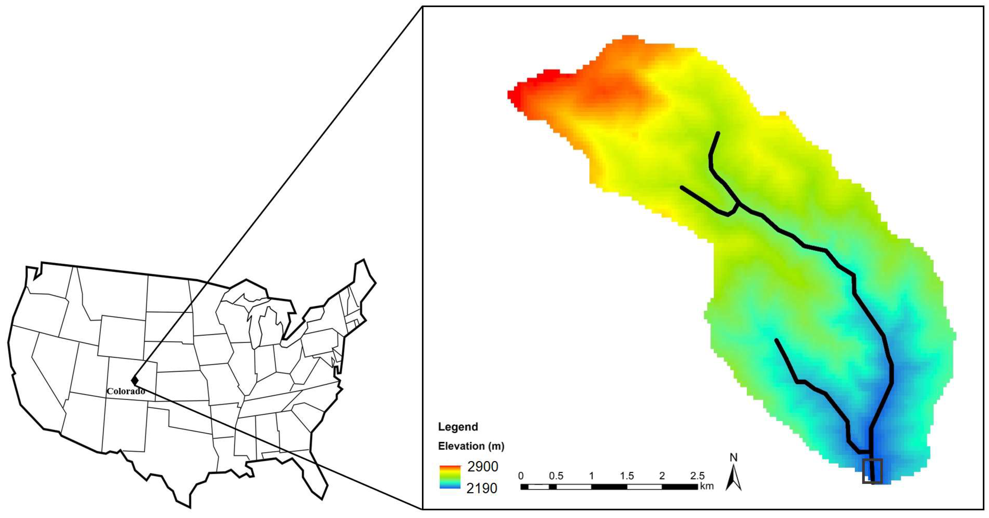
4.1. Background for Test Case Study Area

TLS data acquired following a wildfire disturbance in Colorado, USA [5] provided a test case to compare the analysis methods reviewed in this paper and illustrate the workflow presented in Section 3 (Figure 1 and Table 1). The 2012 Waldo Canyon Fire occurred in Pike National Forest, northwest of Colorado Springs, Colorado in El Paso County [43]. This study utilized data collected as part of a larger investigation of the response of mountain streams following the Waldo Canyon Fire, described in Chin et al. [44]; Kinoshita et al. [45]; and Chin et al. [5]. The test presented here focused on a channel reach in the downstream portion of the Williams watershed (Figure 2), with a drainage area of 4.87 km2. This study reach, henceforth referred to as “Williams Downstream,” has a length of 165 m and encompasses “Willis Reach” described in Chin et al. [5]. Ground-based laser scanning of this study reach provided the data for a comparison of each change estimation method and errors. We demonstrate the steps outlined for the workflow in order: (1) data acquisition, (2) preparation, (3) change estimation and analysis, and (4) error analysis.

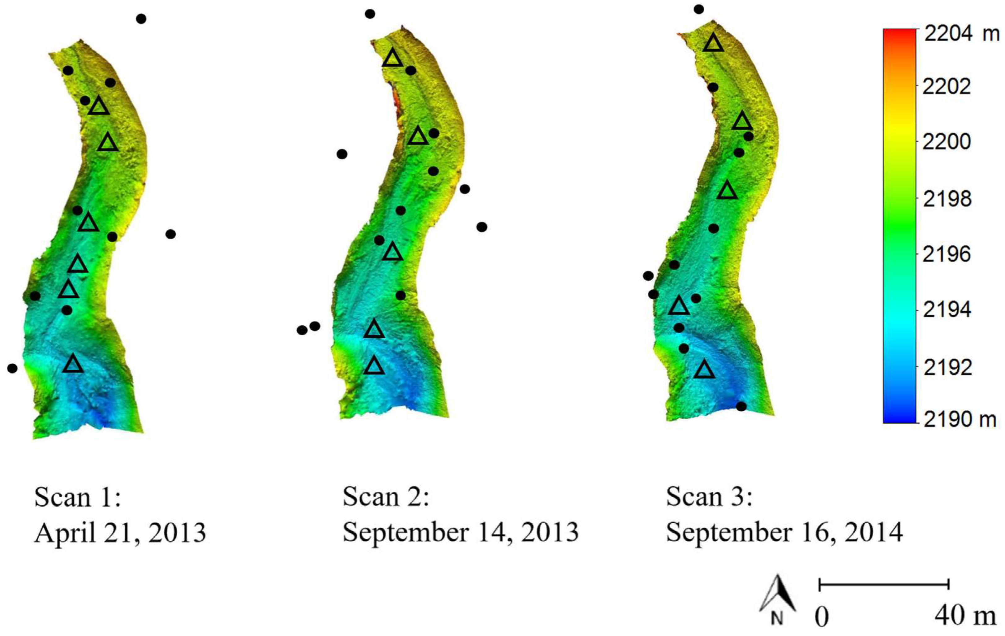
4.2. TLS Data Acquisition

UNAVCO collected TLS data from Williams Downstream reach using a Riegl VZ-400 scanner with a Nikon D700 20 mm camera mounted on a tripod. The scanner system operated in a near-infrared wavelength (800–1000 nm) and the maximum scanner range of data collection varied from 60 to 600 m, depending on object brightness. This setup allowed a 360-degree panorama scan in the horizontal direction and 100 degree in the vertical direction, which measured at a rate of up to 122,000 measurements/sec. The data coverage depended on the incident angle of the laser, as determined by the height of the scanner above the ground and the clarity of the site with respect to the scanner (obliqueness) [46]. The minimum horizontal and vertical step size is 0.0024 degrees. The beam divergence angle and diameter at exit is 0.3 mrad and 7 mm, respectively with a laser beam focal spot at 50 m distance of 18 mm. The maximum measurement rate is 300 kHz. The scanner accuracy (the difference between the true value and measured value) was ± 5 mm, and the precision, or repeatability, was ±3 mm [46]. Each scan collected approximately 30–33 million points of the hillslope and channel. Multiple scans collected expanded the range and density of the data points and removed or minimized shadowing effects. The additional scan locations provided overlapping data points, which enabled registration of the point clouds for developing a topographic surface of the study reach with an average point density of 20 points/m2.
The first set of TLS datasets collected in April 2013 comprised six separate scans of the Williams Downstream reach. The second and third TLS data sets consisted of five separate scans of the Williams Downstream reach. These scans were collected in September 2013 and September 2014, respectively. Scanner instrument locations are illustrated on Figure 3.

4.3. Data Preparation

All the scans from Williams Downstream were registered and georeferenced. Five to six scans were registered based on tie points as reference points, which were fixed control points and managed by a tie point list (TPL) or log of the data collection to align the single scans of the stream reach. The scans were located in the same coordinate system (project coordinate system), one point cloud was fixed and the other point clouds were transformed to fit the target points of the fixed scan [31]. For georeferencing the data, the scan locations were determined by registering the GPS position of the targets to place the point clouds into a global coordinate system in the WGS84 system, UTM Zone 13N.
The octree structure filtered the data points by sub-dividing the points into eight equally sized cubes. The size of the base cube was −10,000 for min x, y, h, and +10,000 for max x, y, h, and the increment value was 0.1 m. A terrain filter tool filtered and removed vegetation, from the data based on the distances of the points from an estimated ground surface. Based on these distances, the points were classified either as “terrain” or as “off-terrain.” The process started from a coarse grid with 0.25 m size. For each cell, the representative point was selected based on the percentile parameter of 1%, and the tolerance factor parameter was ±0.7 m. For fine filtering, the tolerance value was 0.1 m, and the maximum slope angle was 60 degrees.
Triangulating the point clouds utilized a plane triangulation tool to create DEMs. Maximum triangle edge length was 10 m, maximum triangle tilt angle was 90 degrees and minimum triangle angle was 0 degrees. The triangulation was performed for the active channel excluding hillslopes, and with a top view for our case of study. Also, this study avoided smoothing, which would underestimate the ground surface by ~3.5 m.

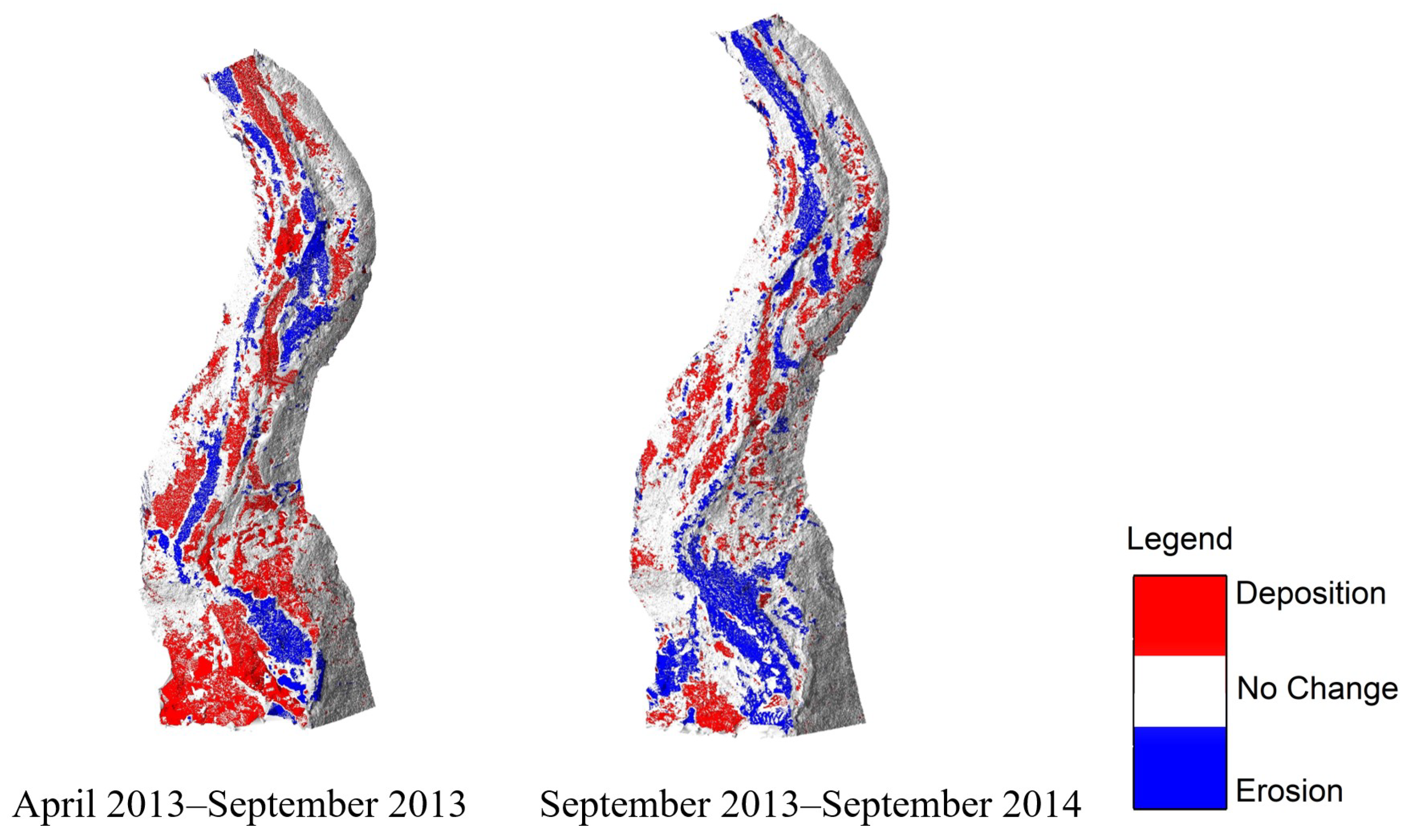
4.4. Change Estimation and Analysis

This comparative analysis calculated the volume between two surfaces (base mesh, reference mesh) based on the DOD method. The two meshes were converted to raster structures with 0.1 m cell size. Three DEMs were derived from the TLS and point cloud preparation for Williams Downstream reach (April 2013, September 2013, and September 2014; Figure 3), which showed the topographic variations within the stream channels. Volumetric changes in channel sediment between scans were calculated by subtracting the DEM of the post-fire, pre-storm from the post-storm DEM [2,11]. We then compared three methods, C2C, C2M, and M3C2, to estimate topographic changes between two successive scans of the same reaches.

4.5. Error Analysis

To quantify the error for two TLS scans between April 2013 and September 2013, two point clouds from the regular TLS survey and fixed targets with high resolution [31] were compared. Surveys of fixed targets were not available to evaluate the error for September 2014. Therefore, empirical error was calculated, which was the uncertainty of two point clouds from 12 immovable objects (large boulders) within the overlapping areas represented by adjacent scans (i.e., point offset in any x, y, or h direction) [41,42]. This represented the uniform mean error or average overall error in point clouds including registration error for the reach. The errors in x, y, and h directions were propagated in the temporally separate scans and calculated according to Equation (2).
The DEM error was estimated for each scan (April 2013, September 2013 and September 2014) separately by comparing ten random cross sections of the channels before and after triangulation. The RMSE (Equation (1)) was calculated for each scan, which was used to estimate the total propagated error in a DEM of Difference ( δ h ( D o D ) (Equation (3)) between two successive scans. Finally, Equation (4) provided an estimation of the volumetric error.

5. Application and Performance of the Workflow Methods in Quantifying Changes and Error

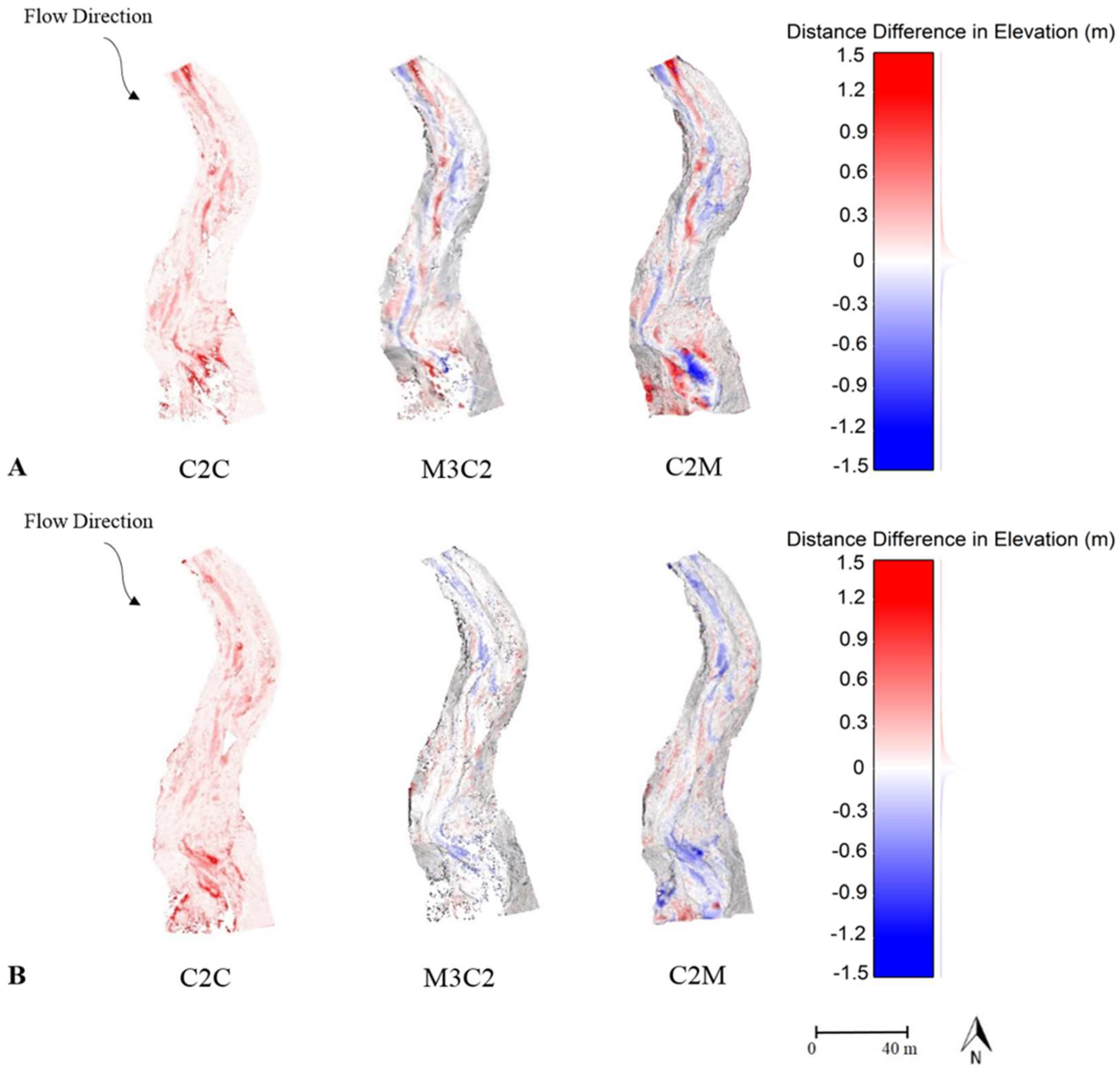
5.1. Comparison of Topographic and Volumetric Change Methods

Using the Riscan Pro DOD method to compare the DEMs of successive scans, the volume of erosion and deposition were estimated as 190 m3 and 460 m3, respectively for April, 2013–September, 2013 (over an area of 4970 m2), and 250 m3 and 180 m3 for September 2013–September 2014 (over an area of 5740 m2). Figure 4 provides a schematic of where erosion and deposition occurred based on the DOD method of comparison within the stream channel for two years following the fire.
Distance difference estimation, which is a quantification of the absolute value of elevation changes within the channel caused by both erosion and deposition, for Williams Downstream reach was performed with the CloudCompare C2C, C2M, and M3C2 methods (Figure 5). Figure 5A compares channel morphological changes between April 2013 and September 2013 for each method. The C2C method only represents the absolute distance difference and does not show the erosion and deposition separately. All red areas are channel variations including both gain and loss (Figure 5A). Also, since C2C compares point clouds, areas with no points are visible along the channel. The M3C2 shows the distance difference of the points and is similar to C2C method. However, the erosion (blue) and deposition (red) are separated. The C2M model is a triangulated distance difference surface that shows erosion (blue) and deposition (red) along the channel. Figure 5B shows the comparison of channel morphology changes between September 2013 and September 2014 for each method. The C2C model provides point cloud comparison results in red as an absolute value (change is not separated by erosion or deposition), indicating only a total change [38]. The M3C2 shows the distance difference result of point clouds comparison and is similar to C2C (based on points comparison). However, M3C2 documents erosion and deposition along the channel separately. The C2M model compares triangulated surfaces and does not have any gaps. The result of distance difference is primarily erosion (values less than 0).
All three models in Figure 5A,B show the same erosion and deposition patterns observed in Figure 4. Noticeable “hot spots” or regions with relatively large deposition or erosion (0.9–1.5 m) indicated are evident (Figure 5A,B), which are artifacts of areas with spares points due to shadows from natural features such as boulders and trees, resulting in gaps in the point cloud. Collecting several scans with different perspectives partially removes shadowing effects. However, areas with low point density may still exist. These areas contribute to the error in DEMs and estimation of channel volumetric changes by introducing errors in data point interpolation.
Estimated net changes (deposition minus erosion) and accumulated changes (deposition plus erosion) allowed comparison across the methods of distance differencing. C2C represents accumulated changes, whereas e C2M and M3C2 represent net change. The DOD method provides both net and accumulated changes. Table 2 shows the net changes in bed elevation and accumulated changes for Williams Downstream reach. For the DOD method, volume is divided by area. The C2C, C2M, and M3C2 methods estimate a mean distance difference based on a Gauss distribution, a continuous distribution of data as a symmetrical bell-shaped graph. These results provide a basic comparison of different methods for estimating surface variations. The distance differences in elevation from each method has a relatively small absolute value range between 0.009 and 0.150 (Table 2). The net changes during September 2013–September 2014 for DOD and M3C2 methods are the same (0.054 m), and the maximum difference is 0.020 m. The only significant difference exists in accumulated changes for September 2013–September 2014, where the value for the C2C method (0.140 m) is almost twice the DOD method (0.075 m). Since the C2C technique is based on the measurement of the closest point distance, the distance estimation between two point clouds is sensitive to the point density. It is only appropriate for very dense point clouds and not an accurate distance measurement method [34,38].

5.2. Comparison of Errors by Method

5.2.1. Error in Point Clouds

The mean uncertainty of two point clouds (April 2013 and September 2013) was estimated based on a comparison of two sets of points from the TLS survey and fine scanning (larger number of points collected) of fixed targets (Figure 3). The resolution of the fine scans from the fixed targets in TLS scanning using a Riegl Scanner was 9 to 555 points, whereas the resolution of the fixed targets for the same area with fine scanning mode was 2106 to 319,394 points. Thus, the fine scans from the fixed targets were considered as the reference data and presumably error free [35]. However, it should be noted that the resolution of scans can be different based on the TLS instrument and analysis software system used.
The error analysis was performed to evaluate uniform error for the September 2014 scan data with no fixed target by comparing points from stationary rocks in overlapping area (Figure 3). RMSE was estimated for each scan in x, y, and h directions (Table 3). The values range from 0.003 m to 0.008 m for all three scans and demonstrate that the TLS survey methodology has a low overall uniform error regardless of the interpolation technique.
The errors in x, y, and h directions were propagated and estimated as 0.015 m for April 2013–September 2013, and 0.016 m for September 2013–September 2014 (from Equation (2)). This procedure yields an estimate of minimum LoD. The LoDmin of points is important in the C2C and M3C2 methods, which are based on comparing point clouds to estimate the distance differences. Consequently, in the C2C and M3C2 methods, any change estimation should be subtracted from 0.015 m (for April 2013–September 2013) or 0.016 m (for September 2013–September 2014) to incorporate the uncertainty. Also, change estimated below 0.015 m or 0.016 m should be excluded from analysis and results.

5.2.2. Error Analysis after Triangulation (DEM Error)

The interpolation error was estimated for each scan (April 2013, September 2013, and September 2014) by comparing the actual points with its triangulated surface (Table 4). The estimated RMSE of the DEMs is 0.009–0.014 m, which is relatively larger compared to the RMSE of the point clouds (0.003–0.008 m; Table 3). This result indicates that triangulation of the point clouds increases the error, specifically in areas with large gaps due to the interpolation of points. The triangulation error can depend on the algorithm used for converting point cloud to DEM. However, the same workflow to estimate errors is encouraged for all processing algorithms. The propagation of DEM error for each scan utilized Equation (3) to calculate the potential error in distance difference of two successive scans, which is the LoDmin for DOD and C2M methods. The LoDmin for April 2013–September 2013 is 0.018 m, and for September 2013–September 2014 is 0.017 m. Similar to LoDmin calculated for points, change estimates for DOD and C2M should be subtracted from 0.018 m (for April 2013–September 2013) or 0.017 m (for September 2013–September 2014) to incorporate uncertainty. Additionally, the DOD and C2M analysis results should exclude any changes estimated below 0.018 m or 0.017 m.

5.2.3. Volumetric Error

Estimation of the volumetric error utilized Equation (4) to determine the uncertainties found in the volumetric calculations. Considering the entire volume of the channel, the volumetric error (δυ) is 89.5 m3 (0.03%) for April 2013–September 2013 for a total volume of 2.92 × 10⁵ m3, and 97.6 m3 (0.032%) for September 2013–September 2014 for a total volume of 3.02 × 10⁵ m3. The volumetric error of the erosion and deposition was estimated as a proportion of the channel volume and is 190 ± 0.06 m3 and 460 ± 0.14 m3, respectively, for April 2013–September 2013, and 250 ± 0.08 m3 (erosion) and 180 ± 0.06 m3 (deposition) for September 2013–September 2014. Since the volumetric error is a proportion of the volume, the error increases with increasing erosion or deposition volume. The volumetric errors are 0.03%–0.032% of the volumetric changes and attributed to existing errors in point clouds and DEMs, which result from triangulation and potential error from data preparation and processing. In comparison to the erosion and deposition volume, these volumetric errors are negligible. Despite the errors in the volumetric change evaluations, TLS provides volume changes within terrain channels with relatively low uncertainty.

5.3. Discussion of Errors

In prior works, researchers have applied Terrestrial Laser Scanning to watersheds after disturbances; however, minimal guidance is available to report errors and uncertainty associated with estimates. Therefore, this step is often left out [3]. This section compares error analysis methods developed in this study with methodologies and results from prior works.
Staley et al. [2] used TLS before and after storms to estimate volume of erosion and deposition in a small (0.01 km2) headwater sub-basin of the Arroyo Seco after the 2009 Station Fire in Los Angeles, California (USA). This investigation incorporated 11 control points (locations scanned in situ and assumed to have minimal errors) within the basin to estimate errors associated with TLS data. Topographic changes ranged from −1.34 ± 0.040 m (erosion) to 1.77 ± 0.040 m (deposition). The minimum level of detectable topographic change was 0.011 m and the authors excluded areas with changes below the 0.011 m threshold from the volumetric analysis [2]. Rengers et al. [13] collected five successive TLS datasets in the Colorado Front Range (USA) and estimated an average erosion along the main channel of 0.073 m with minimal deposition (less than 1 cm). Following Klapinski et al. [42], Rengers et al. [13] estimated the uncertainty of the maximum offset of each TLS point cloud by comparing stationary objects (i.e., large rocks and boulders) with overlapping areas through a fuzzy inference system (FIS) based on Wheaton [47]. An uncertainty between 0.005–0.02 m was estimated as the minimum level of detection, which was assigned to each pixel in the DEM and used as a threshold to remove data from the analysis. Another study by Florsheim et al. [1] incorporated multiple scan positions to construct changes in topography for 176 m of stream channel before and after a storm season, which was used to calculated volumetric change following the 2013 Springs Fire in southern California (USA). The authors utilized error analysis methods similar to the current study to quantify uncertainty in the triangulated surfaces compared to the point cloud data. Florsheim et al. [1] estimated a propagation error of 0.011 m, or ~16% of the total volumetric change resulting from deposition, which is larger than the errors estimated in this study (0.030%–0.032%). This may be due to the number of scan positions used and the amount of volumetric change observed within the reach.
In general, studies [1,2,13] that quantified errors in TLS datasets often utilized a variety of methods. However, the estimated uncertainty in elevation change ranged from 0.005–0.02 m, which is comparable to the errors quantified in this paper (0.017–0.018 m). Thus, the current study reviewed and discussed the C2C, C2M, M3C2, and DOD methods to provide a workflow for quantifying topographic changes and errors for analyses with multiple datasets.

6. Conclusions

This paper provides a workflow to guide effective and efficient methods to process and interpret LiDAR information and to quantify associated uncertainty. The application of the workflow to TLS data collected after the 2012 Waldo Canyon Fire provided a demonstration of quantifying error in four methods for estimating topographic and volumetric changes in channel sedimentation. This comparison advances our understanding of the extent of error propagation during data preparation and processing.
To summarize the lessons learned from this analysis:
  • The error analysis quantifies a minimum level of detection, which is important for considering the uncertainty in both point clouds and DEMs in TLS processing, analysis results, and conclusions about channel alteration.
  • The error analysis demonstrates rapid propagation of error from individual DEMs into DEMs of difference, highlighting the need for consideration. Estimating errors not only for elevation (h), but also in the horizontal directions (x and y) is necessary in point clouds analysis, especially in complex and rugged terrain. However, errors for each single dataset are significantly smaller in point clouds before triangulation (0.003–0.008 m) than in DEMs (0.009–0.014 m) as converting data points within a LiDAR point cloud to DEMs increases the error by interpolation. The propagated error for comparing multiple datasets recording surfaces over time is similar for point clouds (0.015–0.016 m) and DEMs (0.017–0.018 m).
  • Approximately 0.030%–0.032% of the estimated erosion and deposition results from errors that exist in the TLS data set, indicating a lower potential for uncertainty for estimating volumetric changes.
  • Triangulation of the bare Earth points in the point cloud increases error, especially in complex topography, where occlusions are typically larger than flat surfaces. Therefore, techniques that estimate topographic changes that are solely based on point comparison (i.e., C2C and M3C2) are more reliable than those that interpolate surfaces (i.e., C2M and DOD).
  • The C2C method, the absolute distance difference, does not negative and positive values, making data interpretation challenging for studies that are interested in erosion or deposition. In general, C2C compares the closest point to the reference point and provides a simple method for rapid change estimation.
  • The M3C2 method extracts erosion and deposition rates from point cloud comparisons and calculates the most accurate and reliable results for the comparison of two surfaces (of the methods reviewed in this work). The M3C2 method does not use interpolation, which minimizes the errors present, especially in complex terrain.
  • The C2M and DOD methods are based on triangulated surfaces. The C2M method is recommended to estimate distance difference and provide elevation, whereas the DOD method is recommended for volumetric changes. The DOD estimates are similar to the M3C2 method. The findings of this review and analysis suggest DOD for estimating volumetric changes, and M3C2 for estimating distance differences in elevation in point clouds.
TLS applications have advantages for assessing topographic changes, and for providing three-dimensional surfaces to detect changes with relatively high accuracy. Although this paper compared several methods for topographic and volumetric change and error estimation based on TLS, these methods are also applicable to other high-resolution methods such as aerial-based LiDAR or SfM photogrammetry data analyses. The suggested workflow is especially necessary as point cloud data are increasingly incorporated into research that seeks to improve understanding of short- and long-term changes after disturbance.

Author Contributions

S.N., A.M.K., A.C., and J.L.F. participated in and designed the data review and error analysis presented in this paper. A.C. conceived the idea for and designed the Waldo Canyon post-wildfire geomorphic investigation, performed the TLS data collection (supported by NSF EAR 1254989) and contributed survey equipment, materials, analysis tools, TLS data, and technical knowledge. S.N., A.M.K., and J.L.F. reviewed TLS and uncertainty methods. All authors, S.N., A.M.K., A.C., and J.L.F. equally contributed analysis and review of the TLS data and wrote the paper.

Funding

This research was funded by the San Diego State University College of Engineering and University Grants Program and an award from the National Science Foundation to the University of Colorado Denver (EAR 1254989; PI A. Chin) for collection of TLS data. The APC was funded by the San Diego State University Department of Civil, Construction, and Environmental Engineering.

Acknowledgments

We acknowledge the assistance of numerous individuals, especially Keith Williams of UNAVCO for technical support in collecting and processing the TLS data. The U.S. Forest Service granted access into the burned watershed for data collection.

Conflicts of Interest

The authors declare no conflict of interest. The funding sponsors had no role in the design of the study; in the collection, analyses, or interpretation of data; in the writing of the manuscript, or in the decision to publish the results.

References

  1. Florsheim, J.L.; Chin, A.; Kinoshita, A.M.; Nourbakhshbeidokhti, S. Effect of storms during drought on post-wildfire recovery of channel sediment dynamics and habitat in the southern California chaparral, USA. Earth Surf. Process. Landf. 2017, 42, 1482–1492. [Google Scholar] [CrossRef]
  2. Staley, D.M.; Wasklewicz, T.A.; Kean, J.W. Characterizing the primary material sources and dominant erosional processes for post-fire debris-flow initiation in a headwater basin using multi-temporal terrestrial laser scanning data. Geomorphology 2014, 214, 324–338. [Google Scholar] [CrossRef]
  3. Schmidt, K.M.; Hanshaw, M.N.; Howle, J.F.; Kean, J.W.; Staley, D.M.; Stock, J.D.; Bawden, G.W. Hydrologic conditions and terrestrial laser scanning of post-fire debris flows in the San Gabriel Mountains, CA, USA. In Proceedings of the Fifth International Conference on Debris Flow Hazards Mitigation/Mechanics, Prediction, and Assessment, Padua, Italy, 14–17 June 2011; pp. 583–593. [Google Scholar]
  4. Pelletier, J.D.; Orem, C.A. How do sediment yields from post-wildfire debris-laden flows depend on terrain slope, soil burn severity class, and drainage basin area? Insights from airborne-LiDAR change detection. Earth Surf. Process. Landf. 2014, 39, 1822–1832. [Google Scholar] [CrossRef]
  5. Chin, A.; Solverson, A.P.; O’Dowd, A.P.; Florsheim, J.L.; Kinoshita, A.M.; Nourbakhshbeidokhti, S.; Sellers, S.M.; Tyner, L.; Gidley, R. Interacting geomorphic and ecological response of step-pool streams after wildfire. Geol. Soc. Am. Bull. 2019. [Google Scholar] [CrossRef]
  6. Barnhart, T.B.; Crosby, B.T. Comparing two methods of surface change detection on an evolving thermokarst using high-temporal-frequency terrestrial laser scanning, Selawik River, Alaska. Remote Sens. 2013, 5, 2813–2837. [Google Scholar] [CrossRef]
  7. Lane, S.N.; Richards, K.S.; Chandler, J.H. Developments in monitoring and modelling small-scale river bed topography. Earth Surf. Process. Landf. 1994, 19, 349–368. [Google Scholar] [CrossRef]
  8. LANE, S.N. The use of digital terrain modelling in the understanding of dynamic river channel systems. Landf. Monit. Model. Anal. 1998, 311–342. [Google Scholar]
  9. Heritage, G.L.; Milan, D.J.; Large, A.R.; Fuller, I.C. Influence of survey strategy and interpolation model on DEM quality. Geomorphology 2009, 112, 334–344. [Google Scholar] [CrossRef]
  10. Hodge, R.A. Using simulated terrestrial laser scanning to analyze errors in high-resolution scan data of irregular surfaces. ISPRS J. Photogramm. Remote Sens. 2010, 65, 227–240. [Google Scholar] [CrossRef]
  11. Wheaton, J.M.; Brasington, J.; Darby, S.E.; Sear, D.A. Accounting for uncertainty in DEMs from repeat topographic surveys: Improved sediment budgets. Earth Surf. Process. Landf. 2010, 35, 136–156. [Google Scholar] [CrossRef]
  12. Milan, D.J.; Heritage, G.L.; Large, A.R.; Fuller, I.C. Filtering spatial error from DEMs: Implications for morphological change estimation. Geomorphology 2011, 125, 160–171. [Google Scholar] [CrossRef]
  13. Rengers, F.K.; Tucker, G.E.; Moody, J.A.; Ebel, B.A. Illuminating wildfire erosion and deposition patterns with repeat terrestrial lidar. J. Geophys. Res. Earth Surf. 2016, 121, 588–608. [Google Scholar] [CrossRef]
  14. Lane, S.N.; Westaway, R.M.; Murray Hicks, D. Estimation of erosion and deposition volumes in a large, gravel-bed, braided river using synoptic remote sensing. Earth Surf. Process. Landf. 2003, 28, 249–271. [Google Scholar] [CrossRef]
  15. Milan, D.J.; Heritage, G.L.; Hetherington, D. Application of a 3D laser scanner in the assessment of erosion and deposition volumes and channel change in a proglacial river. Earth Surf. Process. Landf. 2007, 32, 1657–1674. [Google Scholar] [CrossRef]
  16. Passalacqua, P.; Belmont, P.; Staley, D.M.; Simley, J.D.; Arrowsmith, J.R.; Bode, C.A.; Crosby, C.; DeLong, S.B.; Glenn, N.F.; Kelly, S.A. Analyzing high resolution topography for advancing the understanding of mass and energy transfer through landscapes: A review. Earth-Sci. Rev. 2015, 148, 174–193. [Google Scholar] [CrossRef] [Green Version]
  17. Singh, A. Review article digital change detection techniques using remotely-sensed data. Int. J. Remote Sens. 1989, 10, 989–1003. [Google Scholar] [CrossRef]
  18. Tarolli, P. High-resolution topography for understanding Earth surface processes: Opportunities and challenges. Geomorphology 2014, 216, 295–312. [Google Scholar] [CrossRef]
  19. Goyer, G.G.; Watson, R. The laser and its application to meteorology. Bull. Am. Meteorol. Soc. 1963, 44, 564–570. [Google Scholar] [CrossRef]
  20. Arrowsmith, J.R.; Glenn, N.; Crosby, C.J.; Cowgill, E. Current capabilities and community needs for software tools and educational resources for use with LiDAR high resolution topography data. In Proceedings of the OpenTopography Meeting, San Diego, CA, USA, 8 August 2008; Volume 8, p. 2008. [Google Scholar]
  21. Shan, J.; Toth, C.K. Topographic Laser Ranging and Scanning: Principles and Processing; CRC Press: Boca Raton, FL, USA, 2008. [Google Scholar]
  22. Jaboyedoff, M.; Oppikofer, T.; Abellán, A.; Derron, M.-H.; Loye, A.; Metzger, R.; Pedrazzini, A. Use of LIDAR in landslide investigations: A review. Nat. Hazards 2012, 61, 5–28. [Google Scholar] [CrossRef]
  23. Monserrat, O.; Crosetto, M. Deformation measurement using terrestrial laser scanning data and least squares 3D surface matching. ISPRS J. Photogramm. Remote Sens. 2008, 63, 142–154. [Google Scholar] [CrossRef]
  24. Vosselman, G. Slope based filtering of laser altimetry data. Int. Arch. Photogramm. Remote Sens. 2000, 33, 935–942. [Google Scholar]
  25. Sithole, G.; Vosselman, G. Experimental comparison of filter algorithms for bare-Earth extraction from airborne laser scanning point clouds. ISPRS J. Photogramm. Remote Sens. 2004, 59, 85–101. [Google Scholar] [CrossRef]
  26. Entwistle, N.; Heritage, G.; Milan, D. Recent remote sensing applications for hydro and morphodynamic monitoring and modelling. Earth Surf. Process. Landf. 2018, 43, 2283–2291. [Google Scholar] [CrossRef]
  27. Brodu, N.; Lague, D. 3D terrestrial lidar data classification of complex natural scenes using a multi-scale dimensionality criterion: Applications in geomorphology. ISPRS J. Photogramm. Remote Sens. 2012, 68, 121–134. [Google Scholar] [CrossRef] [Green Version]
  28. Collins, B.D.; Brown, K.M.; Fairley, H.C. Evaluation of Terrestrial LIDAR for Monitoring Geomorphic Change at Archeological Sites in Grand Canyon National Park, Arizona; US Geological Survey: Reston, VA, USA, 2008.
  29. Brasington, J.; Rumsby, B.T.; McVey, R.A. Monitoring and modelling morphological change in a braided gravel-bed river using high resolution GPS-based survey. Earth Surf. Process. Landf. 2000, 25, 973–990. [Google Scholar] [CrossRef]
  30. Fuller, I.C.; Large, A.R.G.; Charlton, M.E.; Heritage, G.L.; Milan, D.J. Reach-scale sediment transfers: An evaluation of two morphological budgeting approaches. Earth Surf. Process. Landf. 2003, 28, 889–903. [Google Scholar] [CrossRef]
  31. Riegl, J.; Studnicka, N.; Ullrich, A. Merging and processing of laser scan data and high-resolution digital images acquired with a hybrid 3D laser sensor. In Proceedings of the CIPA 2003 XIXth International Symposium, Antalya, Turkey, 30 September–4 October 2003; pp. 511–516. [Google Scholar]
  32. Riegl. Available online: http://www.riegl.com (accessed on 4 June 2016).
  33. Vo, A.-V.; Truong-Hong, L.; Laefer, D.F.; Bertolotto, M. Octree-based region growing for point cloud segmentation. ISPRS J. Photogramm. Remote Sens. 2015, 104, 88–100. [Google Scholar] [CrossRef]
  34. Girardeau-Montaut, D.; Roux, M.; Marc, R.; Thibault, G. Change detection on points cloud data acquired with a ground laser scanner. Int. Arch. Photogramm. Remote Sens. Spat. Inf. Sci. 2005, 36, W19. [Google Scholar]
  35. Fisher, P.F.; Tate, N.J. Causes and consequences of error in digital elevation models. Prog. Phys. Geogr. 2006, 30, 467–489. [Google Scholar] [CrossRef]
  36. Field, D.A. Laplacian smoothing and Delaunay triangulations. Int. J. Numer. Methods Biomed. Eng. 1988, 4, 709–712. [Google Scholar] [CrossRef] [Green Version]
  37. Lee, D.-T.; Schachter, B.J. Two algorithms for constructing a Delaunay triangulation. Int. J. Comput. Inf. Sci. 1980, 9, 219–242. [Google Scholar] [CrossRef]
  38. Lague, D.; Brodu, N.; Leroux, J. Accurate 3D comparison of complex topography with terrestrial laser scanner: Application to the Rangitikei canyon (NZ). ISPRS J. Photogramm. Remote Sens. 2013, 82, 10–26. [Google Scholar] [CrossRef]
  39. Brasington, J.; Langham, J.; Rumsby, B. Methodological sensitivity of morphometric estimates of coarse fluvial sediment transport. Geomorphology 2003, 53, 299–316. [Google Scholar] [CrossRef]
  40. Gens, R. Quality assessment of interferometrically derived digital elevation models. Int. J. Appl. Earth Obs. Geoinformation 1999, 1, 102–108. [Google Scholar] [CrossRef]
  41. Kaplinski, M.; Hazel, J.E., Jr.; Grams, P.E.; Davis, P.A. Monitoring Fine-Sediment Volume in the Colorado River Ecosystem, Arizona: Construction and Analysis of Digital Elevation Models; US Geological Survey: Reston, VA, USA, 2014. [Google Scholar]
  42. Collins, B.D.; Corbett, S.C.; Fairley, H.C.; Minasian, D.L.; Kayen, R.; Dealy, T.P.; Bedford, D.R. Topographic Change Detection at Select Archeological Sites in Grand Canyon National Park, Arizona, 2007–2010; US Geological Survey: Reston, VA, USA, 2012. [Google Scholar]
  43. Young, D.; Rust, B.; Team, W.C.B. Waldo Canyon Fire—Burned Area Emergency Response Soil Resource Assessment; USDA Forest Service, Region 5: Redding, CA, USA, 2012. [Google Scholar]
  44. Chin, A.; An, L.; Florsheim, J.L.; Laurencio, L.R.; Marston, R.A.; Solverson, A.P.; Simon, G.L.; Stinson, E.; Wohl, E. Investigating feedbacks in human–landscape systems: Lessons following a wildfire in Colorado, USA. Geomorphology 2016, 252, 40–50. [Google Scholar] [CrossRef]
  45. Kinoshita, A.M.; Chin, A.; Simon, G.L.; Briles, C.; Hogue, T.S.; O’Dowd, A.P.; Gerlak, A.K.; Albornoz, A.U. Wildfire, water, and society: Toward integrative research in the “Anthropocene”. Anthropocene 2016, 16, 16–27. [Google Scholar] [CrossRef]
  46. Riegl. 3D Terrestrial Laser Scanner with Online Waveform Processing; Technology Report; Riegl Laser Measurement Systems: Horn, Austria, 2012. [Google Scholar]
  47. Wheaton, J.M. Uncertainty in Morphological Sediment Budgeting of Rivers. Ph.D. Thesis, University of Southampton, Southampton, UK, 2008. [Google Scholar]
Figure 1. Four-part workflow for (I) LiDAR data acquisition, (II) preparation and processing, (III) change estimation and analysis, and (IV) error analysis.
Remotesensing 11 00586 g001
Figure 2. Williams watershed is located northwest of Colorado Springs (located at the diamond in the map inset). Elevation is shown and tributaries are highlighted in black (source: USGS National Map 30 m digital elevation map). The rectangle near the outlet of the watershed shows the approximate location of Williams Downstream reach (see Figure 3 for an enlargement of the study reach).
Remotesensing 11 00586 g002
Figure 3. Scans of Williams Downstream reach for April 2013, September 2013, and September 2014. The locations of the fixed targets and boulders used in the error analysis are represented by solid black circles. Scanner instrument locations are represented by triangles.
Remotesensing 11 00586 g003
Figure 4. DEM of Difference (DOD) method used to compare successive scans of Williams Downstream reach. Blue and red denote locations of erosion and deposition, respectively.
Remotesensing 11 00586 g004
Figure 5. Comparison of successive scans of Williams Downstream reach, showing the distance difference in elevation using the C2C, C2M, and M3C2 methods for channel changes between (A) April 2013–September 2013 and (B) September 2013–September 2014.
Remotesensing 11 00586 g005
Table 1. LiDAR point cloud analysis methods and products used in the current study.
MethodProductsReference(s)
TLSPoint cloud collectionRiegl, 2012
Tie point listData registration and georeferencingRiegl et al., 2003
Octree methodPoint cloud filtering to decrease the size of dataVo et al., 2015; Girardeau-Montaut et al., 2005
Height difference between two nearby pointsRemove vegetation and obtain the bare ground surfaceVosselman, 2000; Sithole and Vosselman, 2004
Delaunay triangulationGenerate digital elevation modelsField, 1988; Lee and Schachter, 1980
C2C, M3C2, C2MEstimate topographic variationsLague et al., 2013
DODCalculate volumetric changesLane et al., 2003; Milan et al., 2007; Heritage et al., 2009; Wheaton et al., 2010
Uncertainty of two point clouds from immovable objects in overlapping areaEstimate error in point cloudsCollins et al., 2012, Klapinski et al., 2014
Uncertainty of DEMs based on comparison of cross sections before and after triangulationEstimate error in DEMs after point clouds triangulationLague et al., 2013, Florsheim et al., 2017
Error propagationPropagate the errors from point clouds and DEMsStaley et al., 2014; Passalacqua et al., 2015; Lane et al., 2003; Wheaton et al., 2010
Volumetric errorEstimate error in volumetric changesLane et al., 2003; Staley et al., 2014, Florsheim et al., 2017
Table 2. Net changes (deposition minus erosion) and accumulated changes (deposition plus erosion) for Williams Downstream reach April 2013–September 2013 and September 2013–September 2014.
MethodMean Distance Difference in Elevation (m)
April 2013–September 2013September 2013–September 2014
Net ChangesAccumulated ChangesNet ChangesAccumulated Changes
DOD−0.0120.0750.0540.130
C2C-0.140-0.150
C2M−0.020-0.040-
M3C2−0.009-0.054-
Table 3. TLS point cloud uniform uncertainty for the lateral (x, y) and elevation (h) directions for the TLS scans within Williams Downstream reach.
Scans DateRMSE (m)
xyh
April 20130.0070.0070.003
September 20130.0080.0060.004
September 20140.0080.0050.006
Table 4. Root mean square errors for Williams Downstream DEMs after triangulation.
ScansRMSE (m)
April 20130.012
September 20130.014
September 20140.009

