Article

Fully Convolutional Networks and Geographic Object-Based Image Analysis for the Classification of VHR Imagery

Department of Geosciences, Environment & Society, Université Libre de Bruxelles (ULB), Bruxelles 1050, Belgium
*
Author to whom correspondence should be addressed.
Submission received: 31 January 2019 / Revised: 28 February 2019 / Accepted: 7 March 2019 / Published: 12 March 2019
(This article belongs to the Special Issue Object Based Image Analysis for Remote Sensing)

Abstract

:
Land cover Classified maps obtained from deep learning methods such as Convolutional neural networks (CNNs) and fully convolutional networks (FCNs) usually have high classification accuracy but with the detailed structures of objects lost or smoothed. In this work, we develop a methodology based on fully convolutional networks (FCN) that is trained in an end-to-end fashion using aerial RGB images only as input. Skip connections are introduced into the FCN architecture to recover high spatial details from the lower convolutional layers. The experiments are conducted on the city of Goma in the Democratic Republic of Congo. We compare the results to a state-of-the art approach based on a semi-automatic Geographic object image-based analysis (GEOBIA) processing chain. State-of-the art classification accuracies are obtained by both methods whereby FCN and the best baseline method have an overall accuracy of 91.3% and 89.5% respectively. The maps have good visual quality and the use of an FCN skip architecture minimizes the rounded edges that is characteristic of FCN maps. Additional experiments are done to refine FCN classified maps using segments obtained from GEOBIA generated at different scale and minimum segment size. High OA of up to 91.5% is achieved accompanied with an improved edge delineation in the FCN maps, and future work will involve explicitly incorporating boundary information from the GEOBIA segmentation into the FCN pipeline in an end-to-end fashion. Finally, we observe that FCN has a lower computational cost than the standard patch-based CNN approach especially at inference.

Graphical Abstract

1. Introduction

Advances in remote sensing technology have increased the availability of a large volume of remote sensing data with a high spatial resolution. Consequently, the capability of making precise and accurate land cover maps of urban areas has been enhanced. Land cover (LC) maps are useful for various applications such as urban planning, population modelling and socio-economic analysis. In developing countries, such spatial data is often lacking. Very high spatial resolution remote sensing images (VHR) are desirable for urban mapping because they allow for mapping of a higher level of thematic detail of land cover and have a synoptic view of the earth surface. However, a higher resolution also means a larger volume of data to process. In addition, urban areas have a characteristic heterogeneous structure where roofs of buildings have various sizes and are made of different materials, which increases the challenge of mapping. The enormous amount of data and challenging urban fabric in developing countries creates the need for efficient processing algorithms.
VHR imagery often contains limited spectral information and have high spatial resolution. Thus, standard pixel-based classifiers perform poorly because of the high intra-class and low inter-class variance. However, the pixels can be initially grouped into segments according to some homogeneity criteria, which may then be labelled using a trained classifier [1]. This is the principle of Geographical Object-Based Image analysis (GEOBIA) methods which usually perform better than pixel-based classifiers because segments have additional information compared to individual pixels and produce less noisy maps [2]. The extraction of features has been shown to improve the classification performance of both approaches but has often been limited by the high number of free parameters that need to be optimized, the need for domain knowledge and the amount of effort involved. However, these limitations can be circumvented when using deep learning that allows for the automatic learning of the spatial-contextual features from the input data [3].
Convolutional neural networks (CNNs) are a class of deep learning algorithms that have performed well in image classification tasks in the computer vision domain [4] and are being applied for the analysis of remote sensing data. CNNs learn spatial-contextual features in a hierarchical fashion from simple features in the lower layers to abstract features in the deeper layers. In Patch-based CNN architectures, the central pixel is assigned a label for a given input patch [5]. Conversely, a fully labelled image patch is used for training a fully convolutional network (FCN) architecture [6]. The FCN is more computationally efficient than the patch-based CNN when training and testing tiles because no redundant operations are performed on neighboring patches [7,8]. Moreover, the FCN can take in an input of varied spatial dimensions and make a dense prediction (i.e., per-pixel classification) during inference [9]. A detailed review of different CNN models can be found in LeCun et al. [3], Zhu et al. [10], and Schmidhuber [11].
Maps produced by CNNs typically have smoothed edges and rounded corners. One of the reasons for this is the use of downsampling layers which aim to increase the field of view of the CNN over the input data, but at the same time result in loss of high spatial details and localization of object boundaries. This can be quite limiting especially for some land cover classes such as buildings that mostly have sharply defined edges. Different strategies can be implemented to address this issue. In Sherrah [9] and Yu and Koltun [12] atrous convolutions, i.e., convolutional layers that are interspersed with zeros, are used to increase the field-of-view/context without the need of using downsampling layers. In Chen et al. [13] a fully connected conditional random field (CRF) is used to better capture the object boundaries. Another strategy is the use of skip connections to re-introduce high spatial details lost via downsampling [14,15,16]. Skip connections fuse features from lower convolutional layers with the abstract features in the higher convolutional layers, thereby recovering the primitive features from the lower layers. In Marmanis et al. [17], a strategy that involves representing class boundaries explicitly as contour probabilities which are then additionally used in training the CNN is exploited. This paper implements a fully convolutional network that has atrous convolutional layers and skip connections. The output of each convolutional layer has the same spatial resolution as the input image [8,12].
Recent works have aimed to exploit the complementarity of both GEOBIA and CNN in their workflows. For instance, Guirado and Tabik [18] perform object detection of a protected vegetation species from Google Earth® images by fine-tuning an existing patch-based CNN architecture. In Liu et al. [19] and Liu and Abd-Elrahman [20] an FCN with downsampling layers is investigated for the detection of an invasive grass species (i.e., Cogon Grass) in a wetland whereby the main contributions are evaluation of the effect of background information surrounding an object of interest to the FCN classification accuracy and impact of several data augmentation strategies. Further, a refinement of the FCN classified map using segments and assigning a majority class for each of the underlying segments is done. Similarly, an urban mapping application is evaluated in Längkvist et al. [21] using a patch-based CNN and the results post-processed using segments derived from simple linear iterative clustering (SLIC) algorithm. In Fu et al. [22], a patch-based convolutional neural network is used to identify the irregular segmentation objects. However, one of the limitations was that a wrong label could be assigned to the block as the process depended on the center of gravity of the irregular object. The work by Lv et al. [23] explores a technique of majority voting for CNNs for very high resolution image classification. In Zhang et al. [24], a patch-based object based CNN having multiple input windows is used for land use application and majority voting is used to classify the segments. The work of Zhao et al. [25] uses a two-step process to use segmentations to improve the classification results of a FCN that has downsampling layers.
The main aim of this work is to explore further the complementarity of GEOBIA and CNN for the improvement of boundary definition and is an extension of our work previously presented [26]. An experiment is conducted to evaluate the added advantage of skip connections in an FCN architecture. Segmentation is realized using a state-of-the-art semi-automatic processing chain [27] where different scales (thresholds) and minimum number of pixels in a segment are explored. Majority voting is used to classify the segments and the results compared to the FCN. The case study involves land cover mapping of the city of Goma, in the Democratic Republic of Congo. In comparison to other works of GEOBIA and CNN, the contribution of our work is that our FCN makes use of dilated convolutions, a skip architecture and the post-processing is done with an aim to minimize the rounded corners and smoothing of straight edges in the FCN maps, which can improve the ease of utilization in various socio-economic studies. In addition, to the best of our knowledge, it is the first application of FCN and comparison for multi-class LC classification of an urban environment in an African city. Our architecture aims for better edge definition of boundaries of the classes.
The rest of the paper is organized as follows: Section 2 describes the data used and the methodology, Section 3 presents the results while Section 4 provides the discussion, Section 5 presents the summary and future works.

2. Materials and Methods

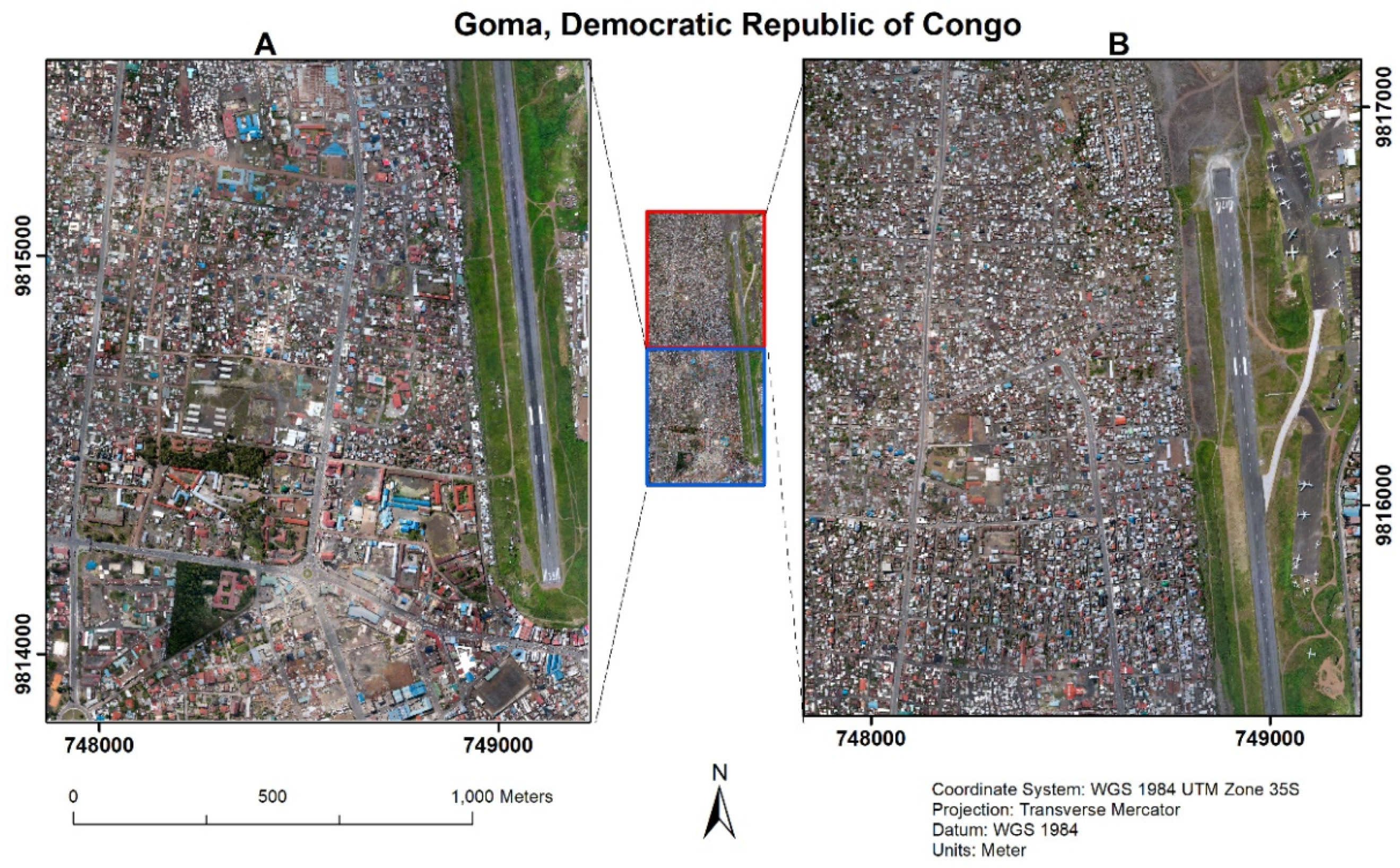
2.1. Data Description

For the experiments, an aerial VHR multispectral image acquired over Goma City, the Democratic Republic of Congo, in 2018 is used as shown in Figure 1.
The image has been orthorectified and comprises three bands namely Red, Green and Blue and has a spatial resolution of 0.175 m. Goma is a city in the North Kivu province and has an approximate population of 800,000 inhabitants. There is a limited availability of high spatial resolution land cover products for the area [28]. The study area as presented in Figure 1 and shows Tile A and Tile B from which training and testing samples are drawn respectively. Each of the tiles covers an area of 1361×1635 m. We consider five land cover classes namely Buildings (BU), Vegetation (VG), Bare Soil (BS), Impervious Surface (IS) and Shadows (SH). 3000 random sampling locations from Tile A are used to provide the training data for both the FCN and GEOBIA approach. In the FCN approach, an image patch of 33 × 33 pixels is extracted around each location and a corresponding fully labelled ground reference image prepared through visual image interpretation by drawing contours around the five classes of interest. For the GEOBIA, a segment is extracted and labelled for each of the location. During testing, 1000 randomly selected and labelled individual pixels from Tile B are used to evaluate the classification methods.

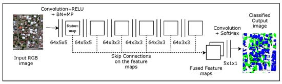
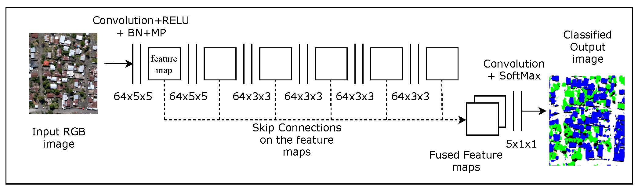
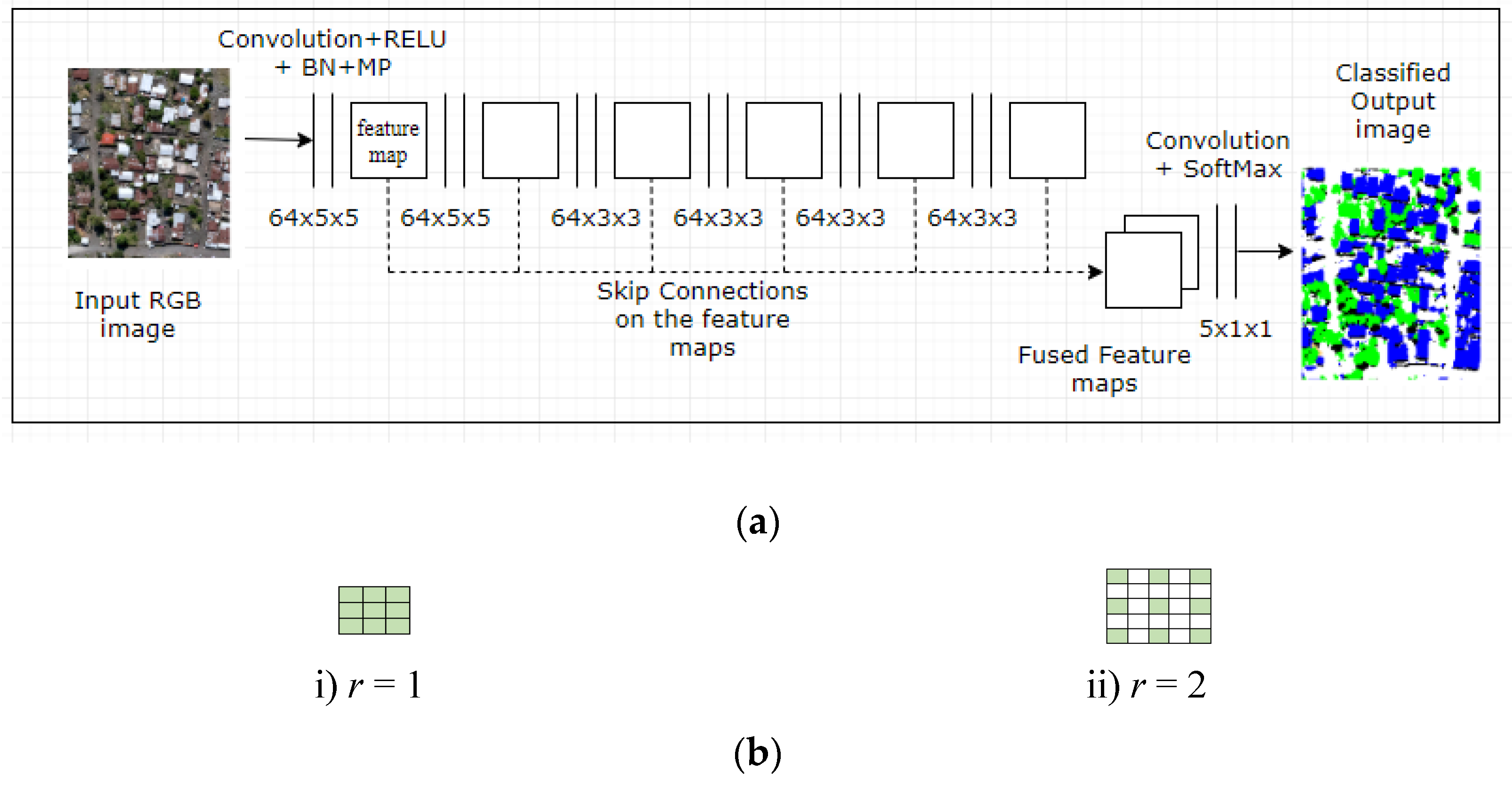
2.2. FCN with Dilated Convolutions and Skip Architecture

The architecture of the implemented FCN is shown in Figure 2a. The building blocks of the architecture are convolutional layers. We make use of atrous (dilated) convolutions that involves interspersing a convolution filter with zeros to increase the receptive field of view without raising the number of parameters [8,12]. For a given filter having spatial dimensions of f × f, a dilated convolution with a rate, r introduces r − 1 zeros between the consecutive elements of the filter. The effective filter dimensions become fe = f + (f − 1) (r − 1). An illustration of a convolutional layer with a dilation rate of 1 and 2 is illustrated in Figure 2b.
Each convolutional layer is comprised of d filters with a spatial dimension of f × f. During a convolution, the filters are shifted through a given number of steps, also called the stride, s of the convolution. Weights and biases are the learnable parameters of the filters. The FCN takes as input a raw image patch with dimension of m × m × d where m is the spatial dimension and d represents the number of channels in the input. A rectified linear unit (RELU) activation function, defined as f(x) = max(0,x) is applied to introduce nonlinearities to the output of the convolution [29]. Batch normalization is then applied to minimize the internal covariate shift during training [30]. Pooling ensures that a dominant signal is propagated to the subsequent layer in the FCN network. In our FCN, we use Maxpooling (MP) with a window size of 2 × 2 and stride s = 1, which ensures that the feature maps are not downsampled. The receptive field of view is rather increased by using dilated convolutions whereby the dilation rate r = 2 in each of the dilated convolutional layers. The spatial dimensions of the feature maps (i.e., outputs of the convolutional layers) are controlled using zero padding and have a dimension of m     f e   + 2 z s × m     f e   + 2 z s × k where z is the number of zeros used to pad the input, fe is the effective filter dimension after dilation, s is the stride of the convolution and k is the number of channels in the feature map.
In the FCN implementation of this paper, the first two convolutional layers have filters with dimension of 64 × 5 × 5 while the subsequent four have filters with a dimension of 64 × 3 × 3 similar to the architecture in Sherrah [9]. During training, the classification loss is given by the cross-entropy function given by:
L ( w ) =   1 N n = 1 N c = 1 C y n c ln ( y ^ n c )      
where n is the number of pixels in mini-batch (i.e., a small subset of the training data), c is the number of classes,   y n c is the vector of true labels and y ^ n c is the vector of predicted labels. We use stochastic gradient descent (SGD) with the backpropagation algorithm to optimize the learning using a mini-batch of size 128, in 100 epochs and a momentum of 0.9 [31,32]. The learning rate is set at 0.1 for the first 50 epochs and 0.001 for the subsequent epochs. Training is done from scratch and takes approximately 10 min using an 8 GB NVDIA® GTX 1080 GPU. Skip connections are used to concatenate the feature maps of the first six convolutional layers and use them as the input to the last convolutional layer. It involves fusing features from low layers with abstract features from higher layers which is useful in recovering the primitive features learnt in the lower convolutional layers to allow for more regular edges in the classified maps. CNN learns features in a hierarchical fashion, and the abstract features poorly detect object contours and edges [13,17]. The last convolutional layer has filters of dimension 5 × 1 × 1 and is followed by a softmax activation function that gives the class distribution of scores for each input pixel x i , for i = 1 c .
p ( y i | x i ) = exp ( x i ) i = 1   c exp ( x i )
Because of the GPU memory limitations, strips from the testing tile having a height of 100 pixels are loaded sequentially onto the GPU to obtain a prediction, after which all the predictions are merged to generate a fully labeled test tile. Our FCN is implemented using the opensource Python libraries namely Keras and Theano [33,34].

2.3. GEOBIA Semi-Automatic Processing Chain

The GEOBIA methodology is implemented using an open source semi-automated processing chain [27] which integrates GRASS GIS with Python and R programming languages [35,36]. The GRASS module “i.segment” based on region-growing algorithm is used for segmentation [37]. Ideally, an optimal segmentation should create homogeneous segments which are different from their neighbours [38], and should produce a trade-off between over- and under-segmentation. There are two main parameters controlling the behavior of this algorithm: “threshold” and “minsize”. The “threshold” parameter is synonymous with the scale parameter in common software used for segmentation. Its values range between 0 and 1, whereby low values (i.e., close to 0) generates over-segmentation while higher values (i.e., close to 1) results in under-segmentation. On the other hand, the “minsize” parameter determines the minimum number of pixels that can be merged into a segment after the final pass of the region growing algorithm.
The quality of a selected segmentation can have a significant impact on the accuracy of the classification [39] and as such, a robust and time efficient unsupervised segmentation parameter optimization (USPO) approach was undertaken [40]. In the literature, Moran’s I (MI) is used to describe the spectral variability between a segment and its neighbors and is considered an oversegmentation goodness metric while weighted variance (WV) describes the variability within a segment and is considered an undersegmentation goodness metric. From a set of candidate segmentations, we selected the one that maximized the objective function of the F-score [41] which maximizes inter-segment heterogeneity and minimizes intersegment heterogeneity by using normalized WV and Global MI defined as:
MI n = MI max     MI MI max     MI min
WV n = WV max     WV WV max     WV min
where WVn is the normalized WV (or MI), WVmax is the highest WV (or MI) value of all examined segmentations, WV min represents the lowest WV (or MI) value of all selected segmentations and WV describes the WV (or MI) value of the current segmentation [39]. The F-measure is given as:
F opt = ( 1 + a 2 )   WV max     WV a 2     WV max     WV min
The calculations of the F-measure for the candidate segmentations were performed through the “i.segment.uspo” module in GRASS [42]. For comparison between FCN and the baseline classifier, the “minsize” parameter was set at 50, and different threshold values between 0.001 and 0.05 evaluated where the value of 0.018 was obtained. For determining the effect of scale and the “minsize” parameter, the parameter settings are presented in Table 1. Several features were computed on each segment derived from the RGB bands followed by feature selection whereby the informative features were the spectral descriptive features (minimum, median, mean, 1st, 3rd Quantiles, maximum, range, standard deviation, variance) and the geometrical covariates (compactness, fractal dimension, perimeter, area) that were used in training of the classification models [43]. 3000 objects were labeled based on the labels of the randomly sampled and visually labelled training points. The selected features were then used as input to a state-of-the-art supervised machine learning (ML) classifiers, namely Extreme Gradient Boosting (XGBoost). The parameters were optimized by Bayesian optimization for XGBoost [44].

2.4. Refining FCN Maps Using GEOBIA Segments

This step involves overlaying the segments generated in Section 2.3 with the classified map from FCN_skip. Then each segment is labelled with the majority class of the pixels within this segment [45]. This approach is abbreviated as FCN_obia and is illustrated in Figure 3.

2.5. FCN_dec and Patch-Based CNN

State-of-the-art deep learning baseline algorithms are used namely a fully convolutional network based on encoder-decoder network similar to SegNet [15,46] (FCN_dec) and a standard patch-based CNN (PB-CNN) that has a VGG-net type of architecture [47]. The PB-CNN network contains four convolutional layers where the first two convolutional layers have filters of dimensions 32 × 3 × 3 and are followed by a RELU activation function. A maxpooling layer of size 2 × 2 with a stride s = 2 is used to downsample the feature maps. The third and fourth convolutional layers have filters with a dimension of 64 × 3 × 3 and are also followed by a similar maxpooling layer in the first two layers. The output of the convolutional layers is flattened and fed into a fully connected layer having 128 neurons. The last layer comprises a five-class softmax activation function used to predict the label of each pixel. During training, overfitting is mitigated by using dropout of 0.25 and 0.5 in the convolutional layers and the fully connected layers respectively [48]. Also, a learning rate of 0.001 and a learning rate decay of 1 × 10⁻⁴ is used over 100 epochs. A batch size of 32 is used. At inference, the central label for each patch is predicted and a pixelwise land cover map produced using a sliding window [5].
The FCN_dec comprises three convolutional layers with downsampling in the encoding layers, and three transpose convolutional layers in the decoding layers. It is an example of a fully convolutional network and takes in an even input patch with dimensions of 32 × 32 × 3 pixels. All the convolutional layers have filters with a dimension of 64 × 3 × 3. A RELU activation, maxpooling layer of 2 × 2 and stride s = 2 and Batch normalization layers are applied after each of the convolutional and transpose convolutional layers. A five-class softmax activation layer produces two-dimensional prediction map having the same dimension as the input patch. The learning rate is set to 0.1 for the first 50 epochs and 0.001 for the subsequent 50 epochs whereas the batch size is set to 128.

2.6. Overview of Abbreviations

Several abbreviations for each of the experiments conducted in this paper have been used. The classifications of segments with XGBoost are abbreviated as XGB_obia and denotes the baseline classifier of the paper. The experiments done using FCN with skip architecture and without skip architecture are denoted as FCN_skip and FCN_noskip respectively. FCN_obia represents the FCN classification that has been refined using segments in a process of majority voting. FCN_obia_051, FCN_obia_101, FCN_obia_181, FCN_obia_201, FCN_obia_301 represents the use of segments generated using a threshold of 0.005, 0.01, 0.018, 0.02 and 0.03 respectively and ”minsize” = 1. On the other hand, FCN_obia_055, FCN_obia_105, FCN_obia_185, FCN_obia_185, FCN_obia_205 and FCN_obia_305 represents the use of segments generated using a threshold of 0.005, 0.01, 0.018, 0.02, and 0.03 respectively and ”minsize” = 50.

2.7. Computation of Accuracy Metrics and Other Area Metrics
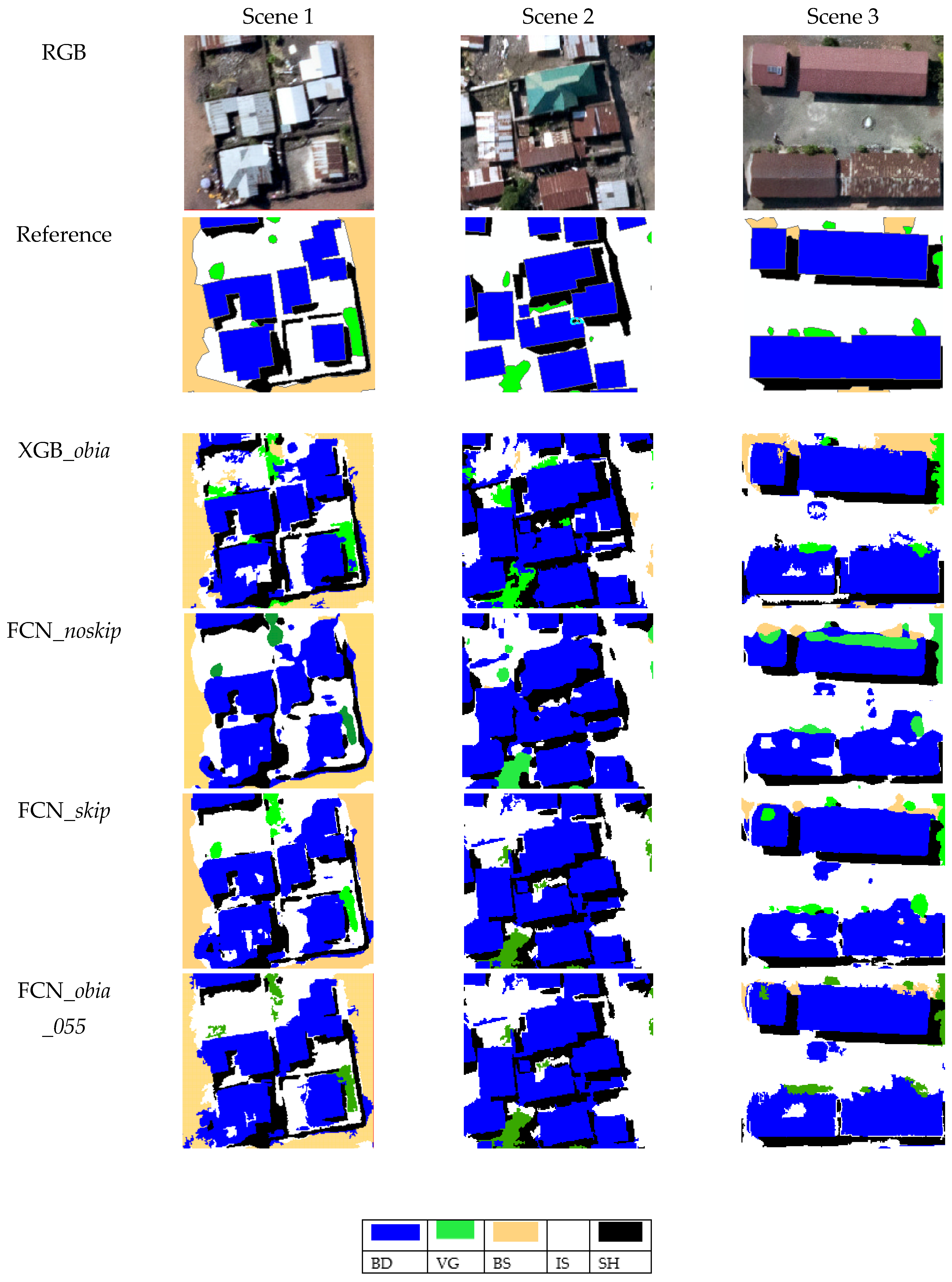
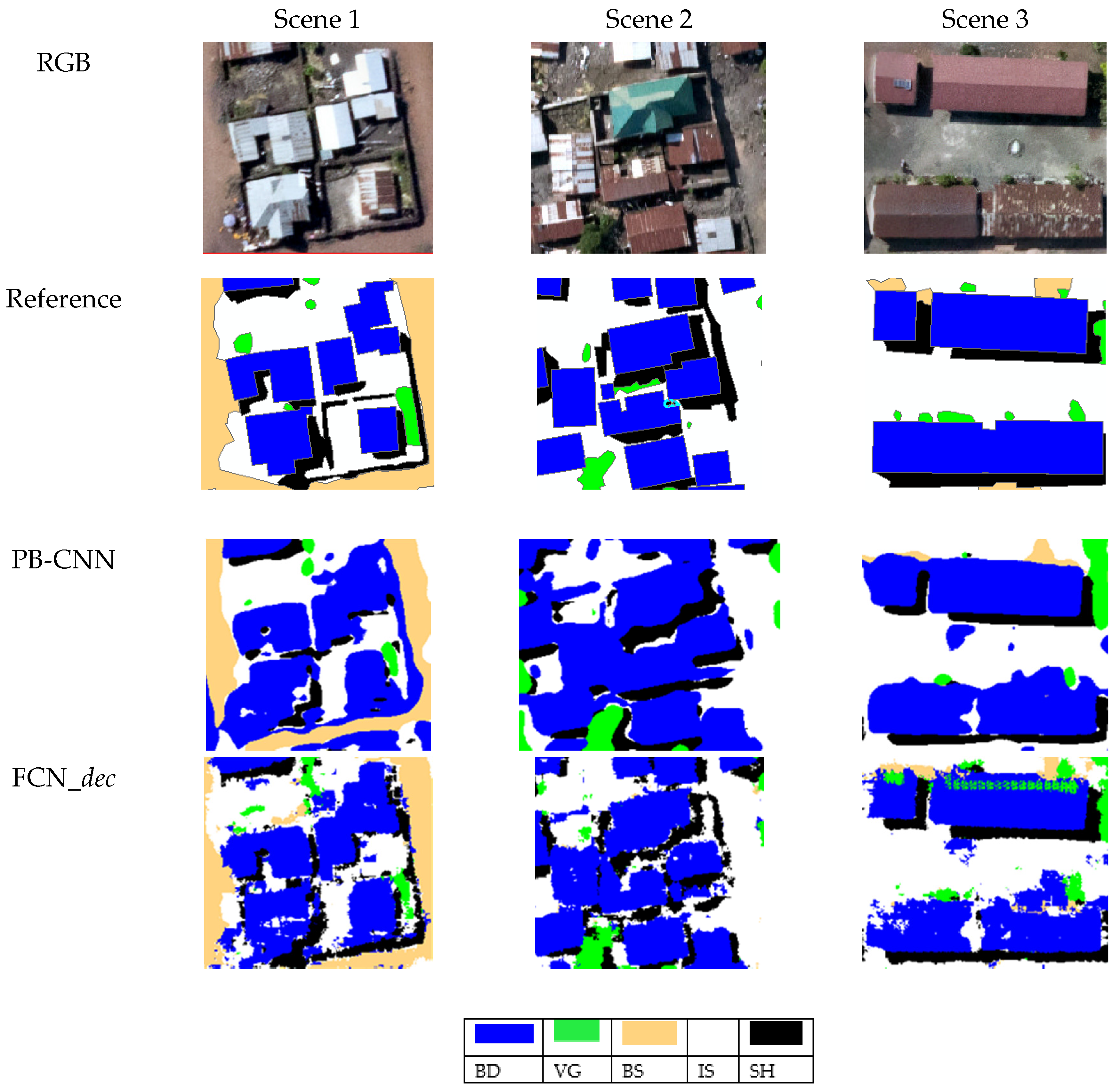
For validation, 1000 points were randomly sampled and labelled using visual image interpretation. In each of the methods, a confusion matrix was produced from which the producer accuracy, the user accuracy, and the overall accuracy were computed [49]. In addition, the overall F1 score for all the classes in each classification method was computed according to the formula:
F 1   score   =   2   ×   precision   ×   recall precision   +   recall
Moreover, the area of the polygons was also evaluated. 60 polygons for the building class were randomly identified and digitized manually. The classified maps of the FCN_skip and FCN_obia were converted to vector format and the corresponding building polygons extracted. Then, the proportion of the area of overlap and the proportion of the area outside the overlapping area with the reference polygon were computed. In Figure 4, the classified area within the reference polygon the classified area outside the reference polygon and the boundary of the reference polygon are shown.
The polygons are likely to have varying sizes; hence we compute the area proportions to allow for comparison. Where IA is the classified area within the reference polygon and EA is the classified area outside the reference polygon, the area proportions are computed as:
Proportion   =   Classified   area   ( IA   or   EA ) Reference   area
Ideally, values of IA should be near one, while values of EA should be close to zero.

3. Results

Accuracy assessment is carried out on an independent test set of 1000 points drawn from Tile B as already mentioned in Section 2.6. In Table 2, the producer accuracy (PA), the user accuracy (UA), the overall accuracy (OA) and the F1 score for the evaluated methods are presented. Generally, high OA and F1 scores are observed for the evaluated methods. The PB-CNN and the FCN_dec have high classification accuracy. Lower classification accuracy is observed in the shadow class by the two methods and can be attributed to the effect of the downsampling layers and the fact that the shadows are linear and cover quite small areas in the image. Nonetheless, high classification metrics are observed in the building class by both methods. XGB_obia has high classification accuracy as segmentations tends to minimize the intra-class variance and maximize between-class variance. The use of skip connections results in better classification accuracy as is seen in the results of the FCN_noskip and FCN_skip which have an OA of 88.2% and 91.30% and F1 score 92.41% and 94.38% respectively. The building class for example benefits from the use of skip connections as the UA and PA are higher in FCN_skip than in FCN_noskip.
The use of segments introduces slight changes in the accuracy metrics. We observe that refining FCN with segments improves mostly the PA and UA of the building class as observed in FCN_obia results. FCN_obia_055 achieves the same OA as the FCN_skip of 91.30 % but has a higher F1-score of 94.87% as compared to 94.38% of the FCN_skip. Meanwhile FCN_obia_101 has an OA of 91.50 % which is not a significant difference. The F1 scores are high but not significantly different.
In Figure 5a, there seems to be less variation in the OA when either a “minsize”=1 or 50 is used. This parameter controls the minimum number of pixels that can be contained in a segment after the last pass of the segmentation algorithm. The use of a suitable segmentation scale implies that after the last pass of the segmentation algorithm, there are unlikely to be many pixels that have not been assigned to a cluster. This implies that few pixels will be clamped into the wrong adjoining cluster. The influence of the threshold parameter can also be observed as presented in Figure 5b. A threshold of 0.005 and 0.5 result in OA of 90.30 % and 76.10% in the FCN_obia results. The scale parameter affects the degree of segmentation, implying that over- or under-segmentation have an influence on the final classification results where GEOBIA segments are used in improving the maps classified using convolutional neural networks.
We also compare the area of the classified buildings to the area of the reference polygons for FCN_skip and FCN_obia_0550 in Figure 6. From the area computations, there is less variation in the area computations between FCN_skip and FCN_obia0550. While the FCN has the advantage of prediction with a high accuracy, the GEOBIA segments produce a more regular map. Combination of both approaches via majority voting can only serve to complement both methods, hence similar area computations. Moreover, the uncertainty inherent in the predictions from either of the approaches was not considered in this work and could be the subject of future works.
A visual assessment on the quality of the classified maps is carried out. Generally, the methods produce high quality maps because the classes are well distinguished in most cases. Several scenes are provided through snippets in Figure 7 and Figure 8. The maps from XGB_obia have better defined edges and corners especially for buildings. The maps from FCN_noskip, FCN_dec and PB-CNN have much more rounded edges as compared to FCN_skip. The maps produced using FCN_obia have better defined edges and corners, which is an improvement when compared to the FCN maps. However, it is observed that the method has challenges especially where there is a misclassification in the FCN. For example, in Scene 3 of the FCN_skip, part of the roof is misclassified as impervious surface. The FCN_obia is unable to correct the misclassification as seen in scene 3 of FCN_obia0550.

4. Discussion

4.1. FCN_dec and PB-CNN

High classification accuracy results and classified maps are obtained by both the FCN_dec and PB-CNN in our experiments. Despite this, a limitation of PB-CNN is the high computation cost at inference. The PB-CNN takes an average of six hours as opposed to FCN_dec that takes an average of 25 min to produce a classified map of Tile B. PB-CNN is limited by the redundant operations that must be performed on the neighboring pixels during training and testing [6,9]. However, there do exist strategies for speeding up the prediction by Patch-based CNN such the “shift-and-stitch” technique [50]. PB-CNN has a lower classification accuracy for the shadow class. In Volpi and Tuia [7], a patch-based CNN had challenges detecting the vehicle class from VHR imagery. The shadows in this study cover smaller and are more linear which may pose a limitation due to use of downsampling layers in the architecture. Lastly, the depth of the network is limited by the size of the input patch. Design of a deeper convolutional network that allows for learning of even more complex features will require a large patch size if it is to contain downsampling layers, but this is accompanied by high cost of computation. Larger filter size also affects the number of parameters and consequently, creates need for more training data and influencing the depth of the network especially if convolutional layers with downsampling layers are used [47]. The FCN_dec design is less flexible than the FCN_skip or FCN_noskip because the downsampling and upsampling layers need to have matching dimensions [8].

4.2. FCN vs. GEOBIA

VHR images pose a classification challenge because of the high intra-class variance and low inter-class variance. In this work, several state-of-the-art approaches have been investigated and metrics such as the overall accuracy, the producer accuracy, the user accuracy and the F1 score computed. In Table 2, high accuracy values are observed which indicates the evaluated approaches perform well in the classification of VHR aerial imagery. The use of a machine learning algorithm to classify segments generated by a semi-automatic processing chain results in high classification accuracy as observed with XGB_obia. The maps from XGB_obia have a good visual quality and better-defined edges as compared to FCN_skip and FCN_noskip. The baseline method used here, namely XGB_obia, performed well because segments have homogeneous characteristics that are more descriptive than individual pixels [51]. This is consistent with literature because the creation of segments aims to group pixels with the goal of minimizing the intra-class variance. Moreover, the extraction of additional features in form of various statistics of the objects which are later used in training the classifier can explain the high accuracy of this approach. The heterogeneous roof structure with different roofing materials such as dust and rust deposits could explain some misclassification in the GEOBIA approach. On the other hand, The FCN learns spatial-contextual features directly from the raw input image in a hierarchical fashion which gives it a better generalization capability.

4.3. FCN_skip vs. FCN_noskip

In this paper, two architectures either with or without skip connections have been investigated. The use of skip architecture helps to recover high spatial information lost through a series of convolution operations. They can recover the basic features learnt in the low convolutional layers by infusing the primitive features from the low layers with the abstract features in the deeper layers, hence better edge detection and numerical accuracy of the classified map [52,53]. The effect of smoothed edges and rounded corners in FCN maps was minimized using skip architecture within the FCN as observed in the classified maps of FCN_skip and FCN_noskip in Figure 7. Although noticeable, this improvement is a slight one.

4.4. FCN_skip vs. FCN_obia

In exploring the complementarity of GEOBIA and FCN based approaches, a series of experiments where segments generated through GEOBIA were combined with the FCN classification are conducted. Although the quantitative improvements are low, the visual quality assessment illustrates a non-negligible improvement. In most cases, there is an improved boundary definition of classes such as buildings. This can be useful in improving the ease of human interpretation, post-processing and shapefile generation of man-made structures. Some classes such as the buildings greatly improve and could be useful in producing high quality built-up products. Indeed, some misclassifications were present, and this could be attributed to the challenging urban fabric characterizing most cities in SSA. Exploring alternative GEOBIA approaches such as joint sparsity approach where a sparse representation of segments is created and used to train a machine learning classifier could be an interesting direction in future works [54,55].
The scale parameter (or threshold) is the most sensitive parameter in the FCN_obia approach. Indeed, the quality of the segmentation will influence the process of majority voting. Large values of scale result in under-segmentation and is accompanied by low classification accuracy as shown in Figure 5b. In addition, better performance could be achieved if the quality of the FCN classification is high with less misclassified pixels. Some of the limitations of the approach include the propagation of uncertainty present in the FCN classification and the GEOBIA classification. Quantifying the uncertainty is beyond the scope of this paper but could form the basis of subsequent works.
In addition to the common accuracy metrics, we evaluated the area of overlap of the classified map in relation to the area of the reference polygons. Comparing the results of the FCN_skip and the FCN_obia, slight differences do appear. Both methods have similar approximations of the area for the classified pixels. Complementarity of GEOBIA and FCN approaches can lead to high accurate maps with better definition of edges [22].
The advantage of deep learning is that it allows for the learning of features directly from the input data in an end-to-end fashion. In Marmanis et al. [17], an edge detector is explicitly incorporated in the FCN classification pipeline. Indeed, the experiments here have demonstrated the added complementarity of FCN and GEOBIA based techniques. The explicit incorporation of the segmentation information might lead to better classification results and is suggested for future works. This might help in constraining the predictions to the structure of the segments.

5. Conclusions

In this work, we have investigated the utility of deep fully convolutional networks for the classification of VHR aerial images of an urban environment in Goma, The Democratic Republic of Congo. Experiments have been conducted using a standard patch-based CNN architecture, an FCN with encoder-decoder architectures, an FCN with and without skip connections and atrous convolutions. Further, baseline experiments using semi-automatic GEOBIA processing chain and a machine learning classifier namely XGBoost have been explored. Lastly, the utility of combining FCN classifications with GEOBIA segments is explored.
To our knowledge, it is the first application of FCN and comparison for multi-class classification for an urban environment of an African city. We also compare the classification results to a state-of-the-art semi-automatic GEOBIA processing chain. We evaluate the accuracy on an independent tile from which no training samples were derived. Lastly, we demonstrate how to improve boundary definition of FCN classification results by using segments which was beneficial for the buildings and impervious ground surfaces. Indeed, the quality of the segmentation has an impact on the refinement process. The high performance of FCN is attributed to the learning of spatial contextual features directly from the input image in an end-to-end fashion. Furthermore, the use of a skip architecture helps to recover the high spatial information from the lower convolutional layers, resulting in an improvement in the classification accuracy. One key point of our approach is the improved classification accuracy of buildings. This is useful for the creation of up-to-date and accurate land cover maps for socio-economic use. The edges are more defined, and the UA and PA increased, although with slight values. One of the future works will involve investigating the propagation of uncertainty in the final classification results. Moreover, explicit incorporation of segmentation results into the deep learning framework would provide another dimension for the integration of GEOBIA based approached and FCN based approaches.

Author Contributions

Conceptualization, N.M., E.W. and M.L.; writing—original draft preparation, N.M.; writing—review and editing, N.M, S.G, T.G, S.V, M.L, E.W.; supervision, E.W and M.L.; project administration, E.W.; funding acquisition, E.W.

Funding

The work presented in the paper is funded by Belgian Science Policy Office (BELSPO) in the frame of the PASTECA project (BR/165/A3/PASTECA).

Acknowledgments

We acknowledge the Royal Museum for Central Africa (RMCA), Belgium for providing the imagery of Goma. We also appreciate the valuable feedback received from the reviewers.

Conflicts of Interest

The authors declare no conflict of interest. The funders had no role in the design of the study; in the collection, analyses, or interpretation of data; in the writing of the manuscript, or in the decision to publish the results.

References

  1. Hay, G.J.; Castilla, G. Geographic Object-Based Image Analysis ( GEOBIA ): A new name for a new discipline. In Object-Based Image Analysis. Lecture Notes in Geoinformation and Cartography; Blaschke, T., Lang, S., Hay, G.J., Eds.; Springer: Berlin/Heidelberg, Germany, 2008. [Google Scholar]
  2. Blaschke, T. Object based image analysis for remote sensing. ISPRS J. Photogramm. Remote Sens. 2010, 65, 2–16. [Google Scholar] [CrossRef]
  3. LeCun, Y.; Bengio, Y.; Hinton, G. Deep learning. Nature 2015, 521, 436–444. [Google Scholar] [CrossRef] [PubMed]
  4. Krizhevsky, A.; Sutskever, I.; Hinton, G.E. ImageNet Classification with Deep Convolutional Neural Networks. In Advances in Neural Information Processing Systems; Pereira, F., Burges, C.J.C., Bottou, L., Weinberger, K.Q., Eds.; Curran Associates, Inc.: Red Hook, NY, USA, 2012; pp. 1097–1105. ISBN 9781627480031. [Google Scholar]
  5. Bergado, J.R.; Persello, C.; Gevaert, C. A deep learning approach to the classification of sub-decimeter resolution aerial images. In Proceedings of the 2016 IEEE International Geoscience and Remote Sensing Symposium (IGARSS), Beijing, China, 10–15 July 2016; pp. 1516–1519. Available online: https://0-ieeexplore-ieee-org.brum.beds.ac.uk/abstract/document/7729387 (accessed on 1 January 2019).
  6. Long, J.; Shelhamer, E.; Darrell, T. Fully convolutional networks for semantic segmentation. In Proceedings of the IEEE Conference on Computer Vision and Pattern Recognition, Boston, MA, USA, 7–12 June 2015; pp. 3431–3440. [Google Scholar]
  7. Volpi, M.; Tuia, D. Dense semantic labeling of sub-decimeter resolution images with convolutional neural networks. IEEE Trans. Geosci. Remote Sens. 2017, 55, 881–893. [Google Scholar] [CrossRef]
  8. Persello, C.; Stein, A. Deep Fully Convolutional Networks for the Detection of Informal Settlements in VHR Images. IEEE Geosci. Remote Sens. Lett. 2017, 14, 2325–2329. [Google Scholar] [CrossRef]
  9. Sherrah, J. Fully Convolutional Networks for Dense Semantic Labelling of High-Resolution Aerial Imagery. Available online: https://arxiv.org/abs/1606.02585 (accessed on 1 January 2019).
  10. Zhu, X.X.; Tuia, D.; Mou, L.; Xia, G.-S.; Zhang, L.; Xu, F.; Fraundorfer, F. Deep learning in remote sensing: a review. IEEE Geosci. Remote Sens. Mag. 2017, 5, 8–36. [Google Scholar] [CrossRef]
  11. Schmidhuber, J. Deep learning in neural networks: An overview. Neural Netw. 2014, 61, 85–117. [Google Scholar] [CrossRef] [PubMed]
  12. Yu, F.; Koltun, V. Multi-scale Context Aggregation By Dilated Convolutions. In Proceedings of the International Conference on Learning and Representations, San Juan, PR, USA, 2–4 May 2016; pp. 1–13. [Google Scholar]
  13. Chen, L.; Papandreou, G.; Kokkinos, I.; Murphy, K.; Yuille, A.L. DeepLab: Semantic Image Segmentation with Deep Convolutional Nets, Atrous Convolution, and Fully Connected CRFs. IEEE Trans. Pattern Anal. Mach. Intell. 2018, 40, 1–14. [Google Scholar] [CrossRef]
  14. Marmanis, D.; Datcu, M.; Esch, T.; Stilla, U. Deep learning earth observation classification using ImageNet pretrained networks. IEEE Geosci. Remote Sens. Lett. 2016, 13, 105–109. [Google Scholar] [CrossRef]
  15. Badrinarayanan, V.; Kendall, A.; Cipolla, R. SegNet: A Deep Convolutional Encoder-Decoder Architecture for Image Segmentation. IEEE Trans. Pattern Anal. Mach. Intell. 2017, 39, 2481–2495. [Google Scholar] [CrossRef]
  16. He, K.; Zhang, X.; Ren, S.; Sun, J. Deep Residual Learning for Image Recognition. In Proceedings of the IEEE Conference on Computer Vision and Pattern Recognition, Las Vegas, NV, USA, 27–30 June 2016; pp. 770–778. [Google Scholar]
  17. Marmanis, D.; Schindler, K.; Wegner, J.D.; Galliani, S.; Datcu, M.; Stilla, U. Classification with an edge: Improving semantic image segmentation with boundary detection. ISPRS J. Photogramm. Remote Sens. 2018, 135, 158–172. [Google Scholar] [CrossRef]
  18. Guirado, E.; Tabik, S. Deep-learning Versus OBIA for Scattered Shrub Detection with Google Earth Imagery: Ziziphus lotus as Case Study. Remote Sens. 2017, 9, 1220. [Google Scholar] [CrossRef]
  19. Liu, T.; Abd-Elrahman, A.; Jon, M.; Wilhelm, V.L. Comparing Fully Convolutional Networks, Random Forest, Support Vector Machine, and Patch-based Deep Convolutional Neural Networks for Object-based Wetland Mapping using Images from small Unmanned Aircraft System. GIScience Remote Sens. 2018, 55, 243–264. [Google Scholar] [CrossRef]
  20. Liu, T.; Abd-Elrahman, A. An Object-Based Image Analysis Method for Enhancing Classification of Land Covers Using Fully Convolutional Networks and Multi-View Images of Small Unmanned Aerial System. Remote Sens. 2018, 10, 457. [Google Scholar] [CrossRef]
  21. Längkvist, M.; Kiselev, A.; Alirezaie, M.; Loutfi, A. Classification and Segmentation of Satellite Orthoimagery Using Convolutional Neural Networks. Remote Sens. 2016, 8, 329. [Google Scholar] [CrossRef]
  22. Fu, T.; Ma, L.; Li, M.; Johnson, B.A. Using convolutional neural network to identify irregular segmentation objects from very high-resolution remote sensing imagery. J. Appl. Remote Sens. 2018, 12, 1. [Google Scholar] [CrossRef]
  23. Lv, X.; Ming, D.; Lu, T.; Zhou, K.; Wang, M.; Bao, H. A New Method for Region-Based Majority Voting CNNs for Very High Resolution Image Classification. Remote Sens. 2018, 10, 1946. [Google Scholar] [CrossRef]
  24. Zhang, C.; Sargent, I.; Pan, X.; Li, H.; Gardiner, A.; Hare, J.; Atkinson, P.M. An object-based convolutional neural network (OCNN) for urban land use classification. Remote Sens. Environ. 2018, 216, 57–70. [Google Scholar] [CrossRef]
  25. Zhao, W.; Du, S.; Emery, W.J. Object-Based Convolutional Neural Network for High-Resolution Imagery Classification Object-Based Convolutional Neural Network for High-Resolution Imagery Classification. IEEE J. Sel. Top. Appl. Earth Obs. Remote Sens. 2017. [Google Scholar] [CrossRef]
  26. Mboga, N.; Georganos, S.; Grippa, T.; Lennert, M.; Vanhuysse, S.; Wolff, E. Fully convolutional networks for the classification of aerial VHR imagery. In Proceedings of the GEOBIA 2018—Geobia in a Changing World, Montpellier, France, 18–22 June 2018; pp. 1–12. [Google Scholar]
  27. Grippa, T.; Lennert, M.; Beaumont, B.; Vanhuysse, S.; Stephenne, N.; Wolff, E. An open-source semi-automated processing chain for urban object-based classification. Remote Sens. 2017, 9, 358. [Google Scholar] [CrossRef]
  28. Michellier, C.; Pigeon, P.; Kervyn, F.; Wolff, E. Contextualizing vulnerability assessment: A support to geo-risk management in central Africa. Nat. Hazards 2016, 82, 27–42. [Google Scholar] [CrossRef]
  29. Glorot, X.; Bengio, Y. Understanding the difficulty of training deep feedforward neural networks. In Proceedings of the Thirteenth International Conference on Artificial Intelligence and Statistics, Sardinia, Italy, 13–15 May 2010; Volume 9, pp. 249–256. [Google Scholar]
  30. Ioffe, S.; Szegedy, C. Batch Normalization: Accelerating Deep Network Training by Reducing Internal Covariate Shift. Available online: https://arxiv.org/abs/1502.03167 (accessed on 1 January 2019).
  31. Bottou, L. Large-scale machine learning with stochastic gradient descent. In Proceedings of the COMPSTAT’2010; Physica-Verlag HD: Heidelberg, Germany, 2010; pp. 177–186. [Google Scholar]
  32. Goodfellow, I.; Bengio, Y.; Courville, A. Deep Learning; MIT Press: Cambridge, MA, USA, 2016. [Google Scholar]
  33. Theano Development Team Theano: A {Python} Framework for Fast Computation of Mathematical Expressions. Available online: http://adsabs.harvard.edu/abs/arXiv:1605.02688 (accessed on 1 January 2019).
  34. Chollet, F.; Others Keras. Github Repos. 2015. Available online: https://github.com/fchollet/keras. (accessed on 28 November 2017).
  35. Neteler, M.; Bowman, M.H.; Landa, M.; Metz, M. GRASS GIS: A multi-purpose open source GIS. Environ. Model. Softw. 2012, 31, 124–130. [Google Scholar] [CrossRef]
  36. R Core Team. R: A Language and Environment for Statistical Computing; R foundation for Statistical Computing: Vienna, Austria, 2015. [Google Scholar]
  37. Momsen, E.; Metz, M. Grass Development Team Module i.segment. In Geographic Resources Analysis Support System (GRASS) Software; Version 7.0; GRASS Development Team: Bonn, Germany, 2015. [Google Scholar]
  38. Haralick, R.M.; Shapiro, L.G. Image Segmentation Techniques. Comput. Vision, Graph. Image Process. 1985, 29, 100–132. [Google Scholar] [CrossRef]
  39. Espindola, G.M.; Camara, G.; Reis, I.A.; Bins, L.S.; Monteiro, A.M. Parameter selection for region-growing image segmentation algorithms using spatial autocorrelation. Int. J. Remote Sens. 2006, 27, 3035–3040. [Google Scholar] [CrossRef]
  40. Georganos, S.; Grippa, T.; Lennert, M.; Vanhuysse, S.; Johnson, B.A.; Wolff, E. Scale Matters: Spatially Partitioned Unsupervised Segmentation Parameter Optimization for Large and Heterogeneous Satellite Images. Remote Sens. 2018, 10, 1440. [Google Scholar] [CrossRef]
  41. Johnson, B.; Xie, Z. Unsupervised image segmentation evaluation and refinement using a multi-scale approach. ISPRS J. Photogramm. Remote Sens. 2011, 66, 473–483. [Google Scholar] [CrossRef]
  42. Lennert, M.; Team, G.D. Addon i.segment.uspo. In Geographic Resources Analysis Support System (GRASS) Software; Version 7.3; GRASS Development Team: Bonn, Germany, 2016. [Google Scholar]
  43. Georganos, S.; Grippa, T.; Vanhuysse, S.; Lennert, M.; Shimoni, M.; Kalogirou, S.; Wolff, E. Less is more: Optimizing classification performance through feature selection in a very-high-resolution remote sensing object-based urban application. GIScience Remote Sens. 2017, 1–22. [Google Scholar] [CrossRef]
  44. Georganos, S.; Grippa, T.; Vanhuysse, S.; Lennert, M.; Shimoni, M.; Wolff, E. Very High Resolution Object-Based Land Use-Land Cover Urban Classification Using Extreme Gradient Boosting. IEEE Geosci. Remote Sens. Lett. 2018, 15. [Google Scholar] [CrossRef]
  45. Zhao, W.; Du, S.; Wang, Q.; Emery, W.J. Contextually guided very-high-resolution imagery classification with semantic segments. ISPRS J. Photogramm. Remote Sens. 2017, 132, 48–60. [Google Scholar] [CrossRef]
  46. Noh, H.; Hong, S.; Han, B. Learning deconvolution network for semantic segmentation. In Proceedings of the IEEE International Conference on Computer Vision, Las Vegas, NV, USA, 11–18 December 2016; pp. 1520–1528. [Google Scholar] [CrossRef]
  47. Simonyan, K.; Zisserman, A. Very Deep Convolutional Networks for Large-Scale Image Recognition. Available online: https://arxiv.org/abs/1409.1556 (accessed on 1 January 2019).
  48. Srivastava, N.; Hinton, G.; Krizhevsky, A.; Sutskever, I.; Salakhutdinov, R. Dropout: A Simple Way to Prevent Neural Networks from Overfitting. J. Mach. Learn. Res. 2014, 15, 1929–1958. [Google Scholar] [CrossRef]
  49. Congalton, R.G. A review of assessing the accuracy of classifications of remotely sensed data. Remote Sens. Environ. 1991, 37, 35–46. [Google Scholar] [CrossRef]
  50. Sermanet, P.; Eigen, D.; Zhang, X.; Mathieu, M.; Fergus, R.; LeCun, Y. OverFeat: Integrated Recognition, Localization and Detection using Convolutional Networks. Available online: https://arxiv.org/abs/1312.6229 (accessed on 1 January 2019).
  51. Blaschke, T.; Hay, G.J.; Kelly, M.; Lang, S.; Hofmann, P.; Addink, E.; Queiroz Feitosa, R.; van der Meer, F.; van der Werff, H.; van Coillie, F.; et al. Geographic Object-Based Image Analysis—Towards a new paradigm. ISPRS J. Photogramm. Remote Sens. 2014, 87, 180–191. [Google Scholar] [CrossRef] [PubMed]
  52. Chen, L.-C.; Papandreou, G.; Kokkinos, I.; Murphy, K.; Yuille, A.L. Semantic Image Segmentation with Deep Convolutional Nets and Fully Connected CRFs. Available online: https://arxiv.org/abs/1412.7062 (accessed on 1 January 2019).
  53. Bergado, J.R.; Persello, C.; Stein, A. Recurrent Multiresolution Convolutional Networks for VHR Image Classification. IEEE Trans. Geosci. Remote Sens. 2018, X, 1–14. [Google Scholar] [CrossRef]
  54. Roscher, R.; Waske, B. Superpixel-based classification of hyperspectral data using sparse representation and conditional random fields. In Proceedings of the 2014 IEEE Geoscience and Remote Sensing Symposium, Quebec City, QC, Canada, 13–18 July 2014; pp. 3674–3677. [Google Scholar]
  55. Dao, M.; Kwan, C.; Koperski, K.; Marchisio, G. A joint sparsity approach to tunnel activity monitoring using high resolution satellite images. In Proceedings of the 2017 IEEE 8th Annual Ubiquitous Computing, Electronics and Mobile Communication Conference (UEMCON), New York, NY, USA, 19–21 October 2017; pp. 322–328. [Google Scholar]
Figure 1. Map illustrating the study area of Goma, Democratic Republic of Congo. The training and testing data are generated from Tile A and Tile B respectively. The images have been provided by the Royal Museum for Central Africa (RMCA), Belgium.
Remotesensing 11 00597 g001
Figure 2. (a) Illustration of implemented FCN. Dilated convolutional layers with a rate, r = 2 are used in the first six convolutional layers. Zero padding of 1 is used in each of the convolutional layers. Maxpooling of 2 × 2 and a stride of 1 is used. In (b) dilated convolution with r = 1 and r = 2 and filter size, f = 3 are illustrated. Key-MP (Maxpooling), RELU (Rectified linear unit), BN (Batch Normalization).
Remotesensing 11 00597 g002
Figure 3. Illustration of the FCN_obia. In (a), the raw image tile is presented, in (b) the segments from OBIA are overlaid over the raw image, in (c) the reference map is shown, in (d) the FCN classified map is shown, in (e) the majority class of pixels from the classified FCN map is assigned to each segment to give a refined map. The classes shown in the legend are: BD-building, VG-vegetation, BS-bare soil, IS-impervious surface and SH-shadows.
Remotesensing 11 00597 g003
Figure 4. Figure illustrating computation of the overlap areas between classified pixels and the reference polygon. Only the building class is evaluated using this metric.
Remotesensing 11 00597 g004
Figure 5. A chart illustrating influence of both scale and the minimum number of pixels in a segment on the overall accuracy (OA) of the FCN_obia approach in (a) and the influence of only the scale parameter in (b).
Remotesensing 11 00597 g005
Figure 6. A chart that illustrates the calculated area proportions for the area of classified pixels outside the reference polygon (EA) and the area of classified pixels within the reference polygon (IA). Both mean and median values are presented to consider any outliers that might be present in the data. The areas have been computed for FCN_skip and FCN_obia0550 experiments.
Remotesensing 11 00597 g006
Figure 7. Classification maps of sample scenes for XGB_obia, FCN_noskip, FCN_skip and FCN_obia methods. BD-Building, VG- Vegetation, BS- Bare Soil, IS- Impervious surfaces, SH- Shadows.
Remotesensing 11 00597 g007
Figure 8. Classification maps of samples scenes for PB-CNN and FCN_dec methods. BD-Building, VG- Vegetation, BS- Bare Soil, IS- Impervious surfaces, SH- Shadows.
Remotesensing 11 00597 g008
Table 1. A presentation of the segmentation parameters used for refining the FCN classification and the assigned acronym.
Scale (threshold)Minsize = 1Minsize = 50
0.005FCN_obia_051FCN_obia_055
0.010FCN_obia_101FCN_obia_105
0.020FCN_obia_201FCN_obia_205
0.030FCN_obia_301FCN_obia_305
0.018FCN_obia_181FCN_obia_185
Table 2. Producer accuracy, user accuracy, overall accuracy and F1 score for the used classification methods (BD: building, VG: vegetation, BS: bare soil, IS: impervious surface and SH: shadows).
BD %VG %BS %IS %SH %OA %F1%
XGB_obiaUA90.0391.6283.1988.5194.7489.5090.18
PA90.3292.6684.6188.2290.91
PB-CNNUA88.1594.4198.6878.6192.8686.9080.37
PA92.9492.3566.3794.9755.32
FCN_decUA92.7192.9090.1178.2790.7887.2091.21
PA89.7492.9072.5794.3062.76
FCN_noskipUA92.5688.7796.2580.2297.3388.2092.41
PA92.2693.7965.8194.2873.74
FCN_skipUA93.9390.9696.7085.4998.8191.3094.38
PA94.8496.6175.2193.2783.84
FCN_obia_055UA94.2790.3798.8085.2498.8191.3094.87
PA95.4895.4870.0995.2983.84
FCN_obia_105UA93.0889.8410084.0898.7590.594.27
PA95.4894.9170.0994.2879.78
FCN_obia_185UA94.8689.4210082.1898.7090.0195.01
PA95.1695.4864.1096.3076.77
FCN_obia_205UA94.2188.4810084.3796.3090.4094.36
PA94.5295.4866.6796.3078.79
FCN_obia_305UA94.8290.8110081.0297.4489.8094.67
PA94.5294.9264.1096.3076.77
FCN_obia_051UA93.9390.9697.7584.9798.8191.2094.38
PA94.8496.6174.3693.2783.84
FCN_obia_101UA93.9790.4898.8885.7698.8191.5094.72
PA95.4896.6175.2193.2783.84
FCN_obia_181UA94.8790.9110084.6898.8091.5095.18
PA95.4896.0572.6595.9582.83
FCN_obia_201UA93.9789.8910084.5997.6290.994.72
PA95.4895.4870.0994.2882.83
FCN_obia_301UA93.9590.9610083.2897.6290.6094.55
PA95.1696.6167.5293.9482.83

