On the Potential of RST-FLOOD on Visible Infrared Imaging Radiometer Suite Data for Flooded Areas Detection

 ,
,  , , ,
, , , 
Abstract
:
1. Introduction
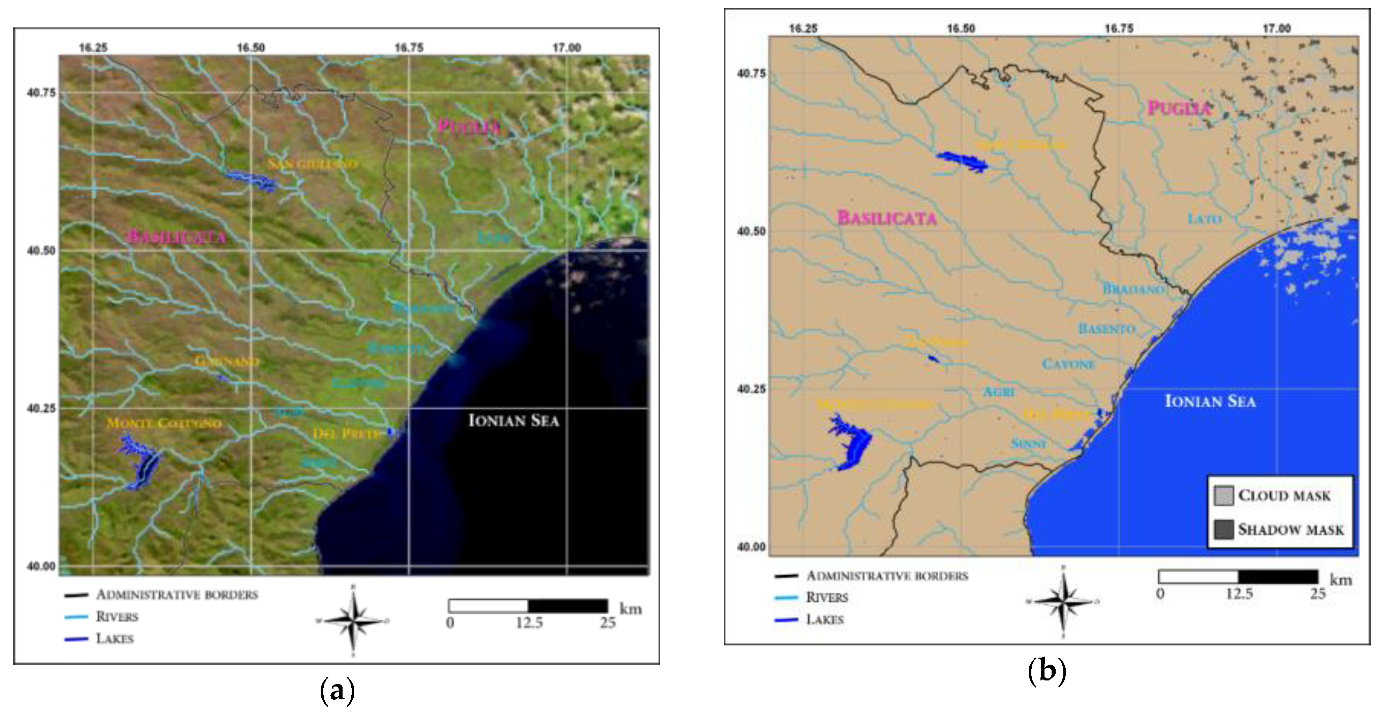
2. The Test Case
3. Data and Methods
3.1. VIIRS Data
3.2. Ancillary Data
3.3. The Robust Satellite Techniques (RST) Approach
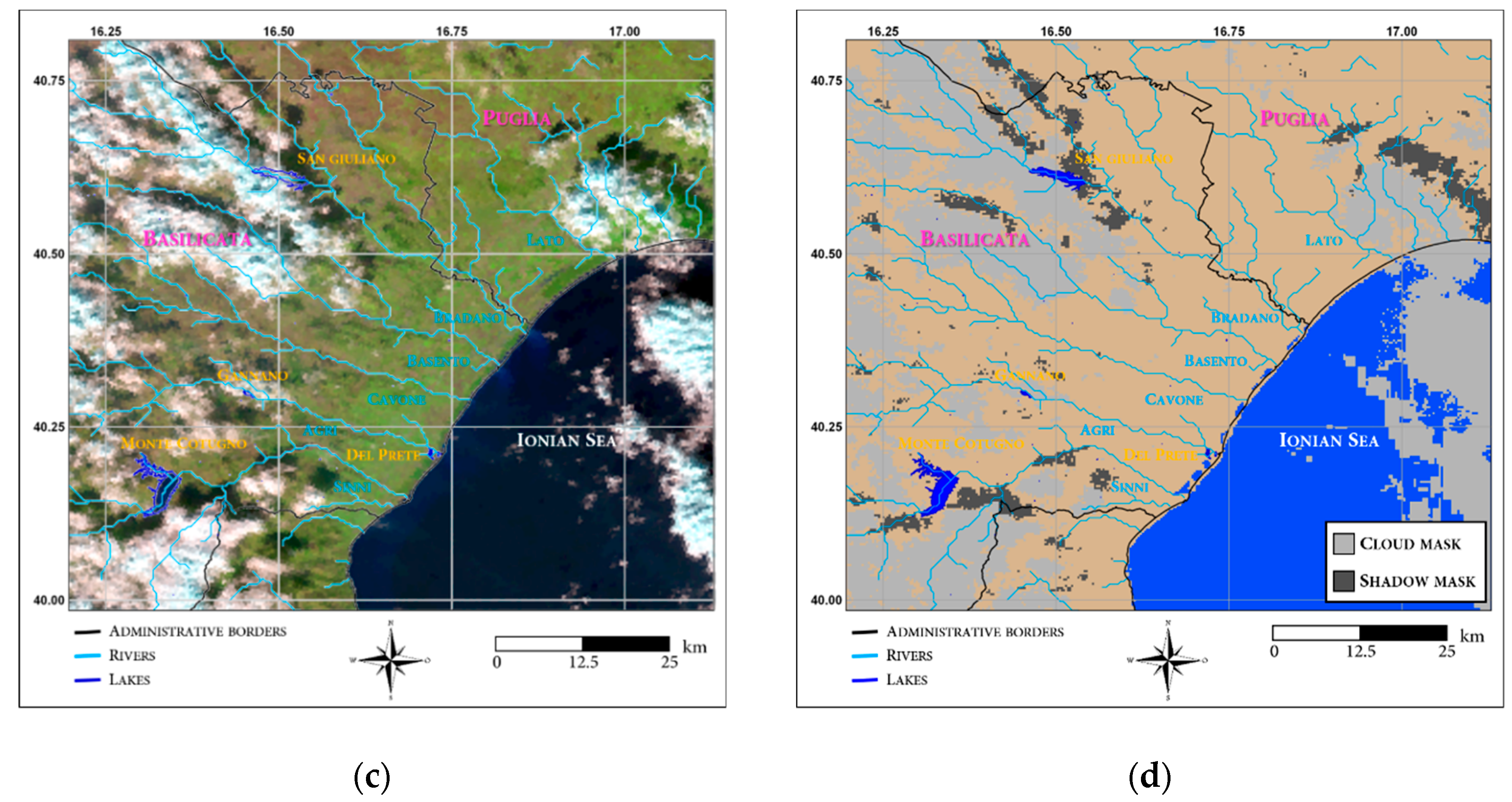
3.4. Cloud Shadows Removal
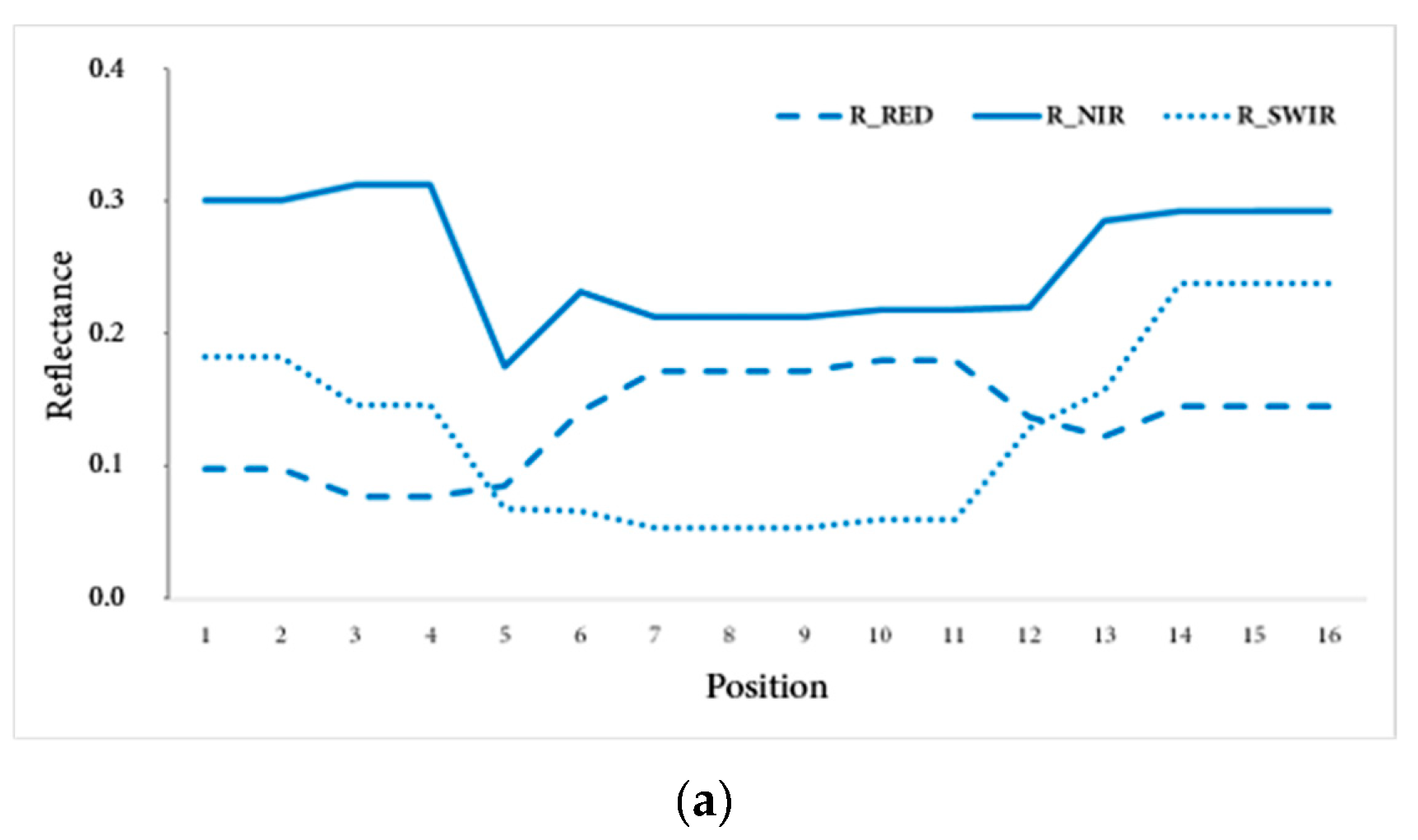
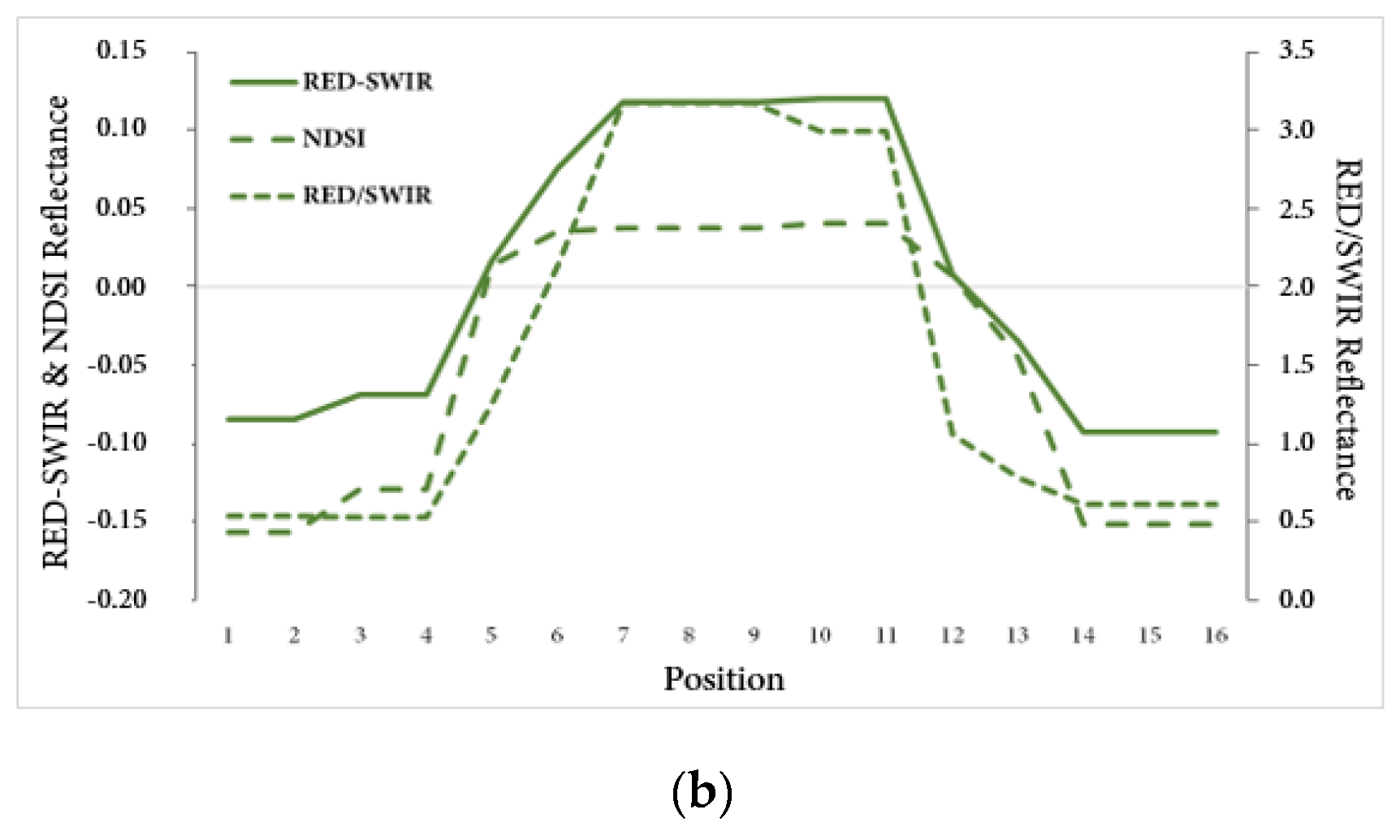
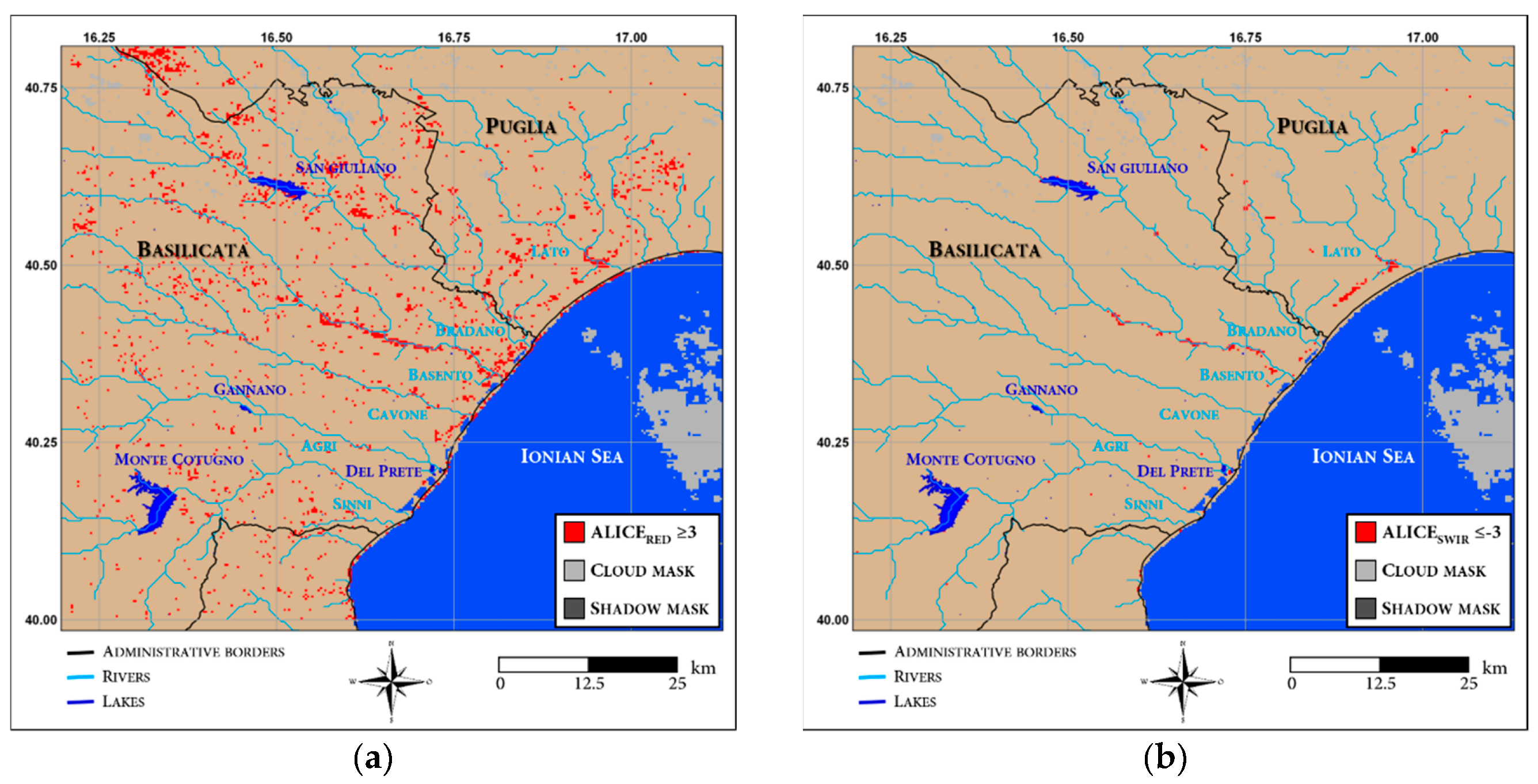
- in the RED (I1), flooded pixels should show higher values of ALICERED than the shadow-affected ones, due to their relative increase in reflectance at this wavelength;
- in the NIR (I2) and SWIR (I3), both flooded and shadow pixels show low (negative) values of ALICENIR and ALICESWIR.
4. Results
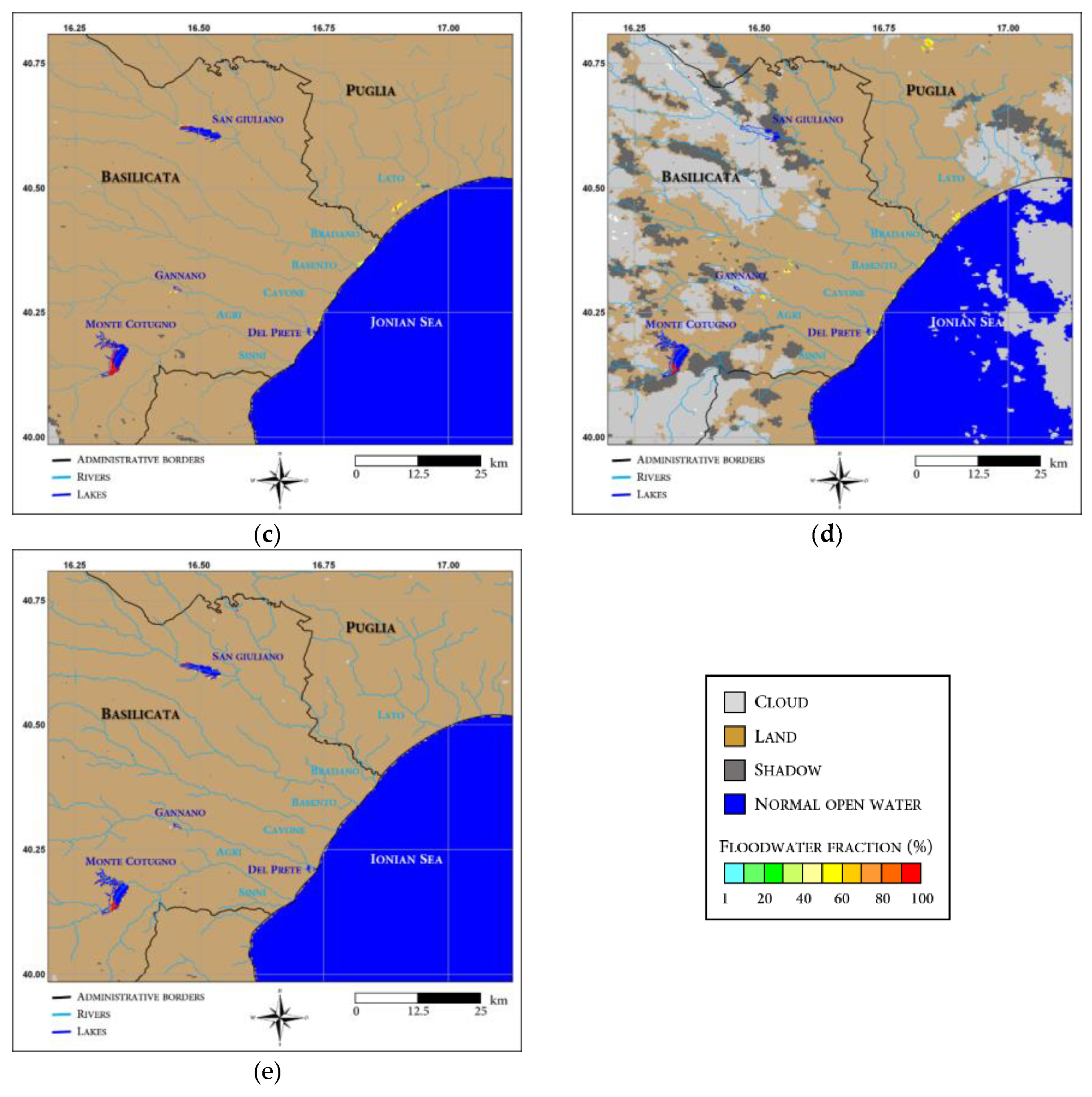
4.1. Cloud Shadow
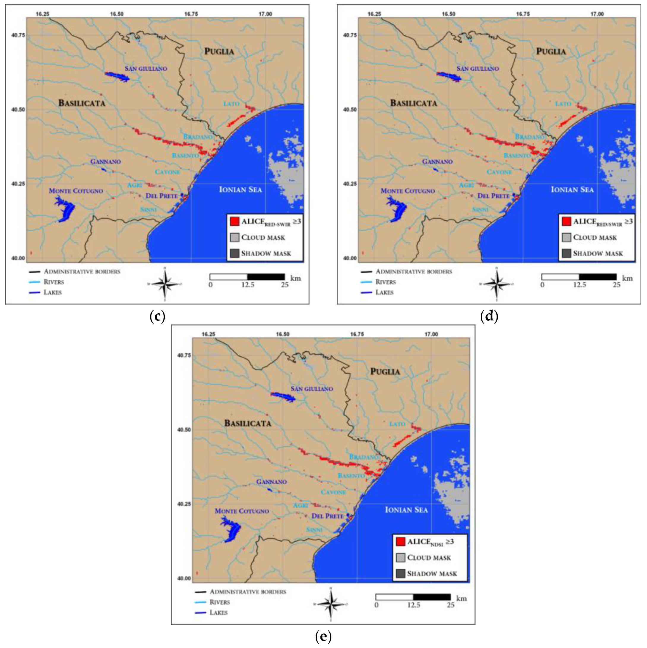
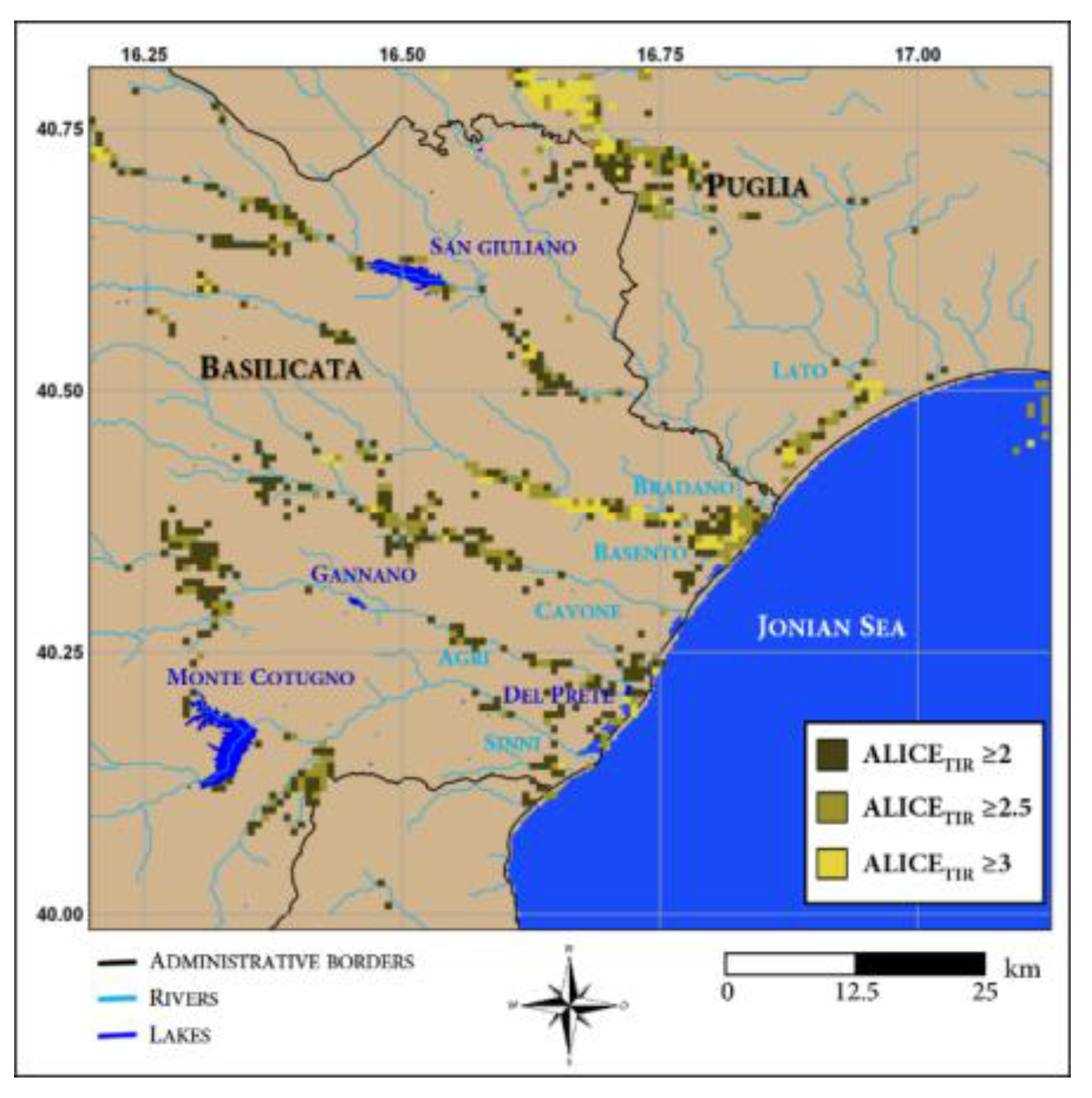
4.2. Selection of the Most Suitable VIIRS RST-FLOOD Indicator
4.3. Assessment Results
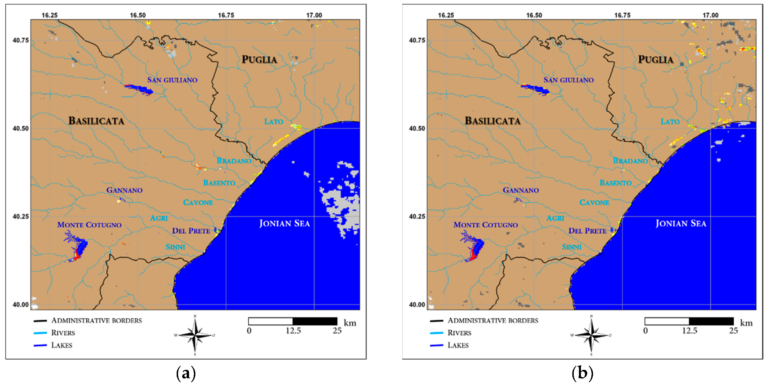
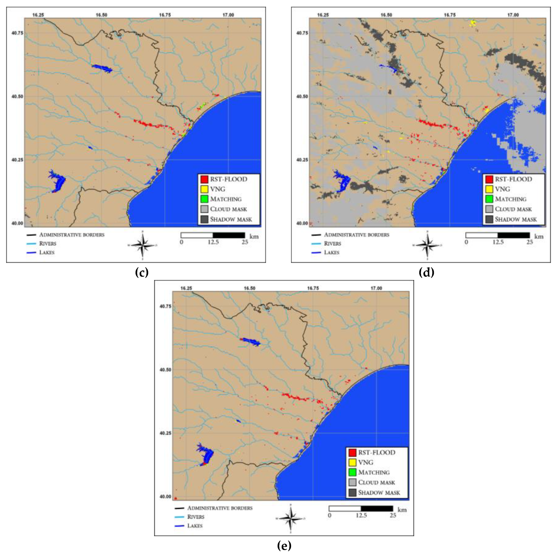
4.3.1. Comparison with Landsat 7 ETM+ Data
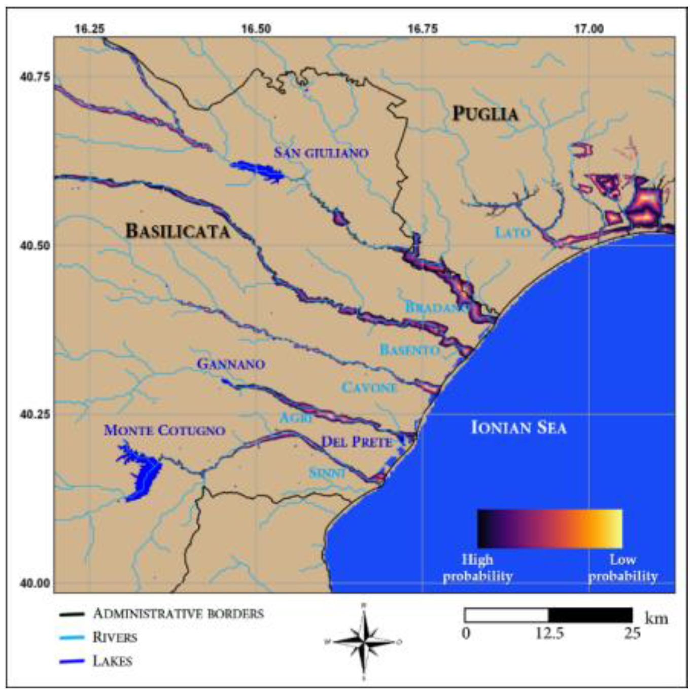
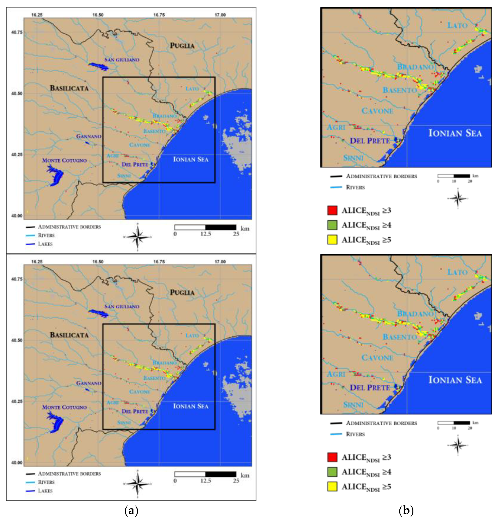
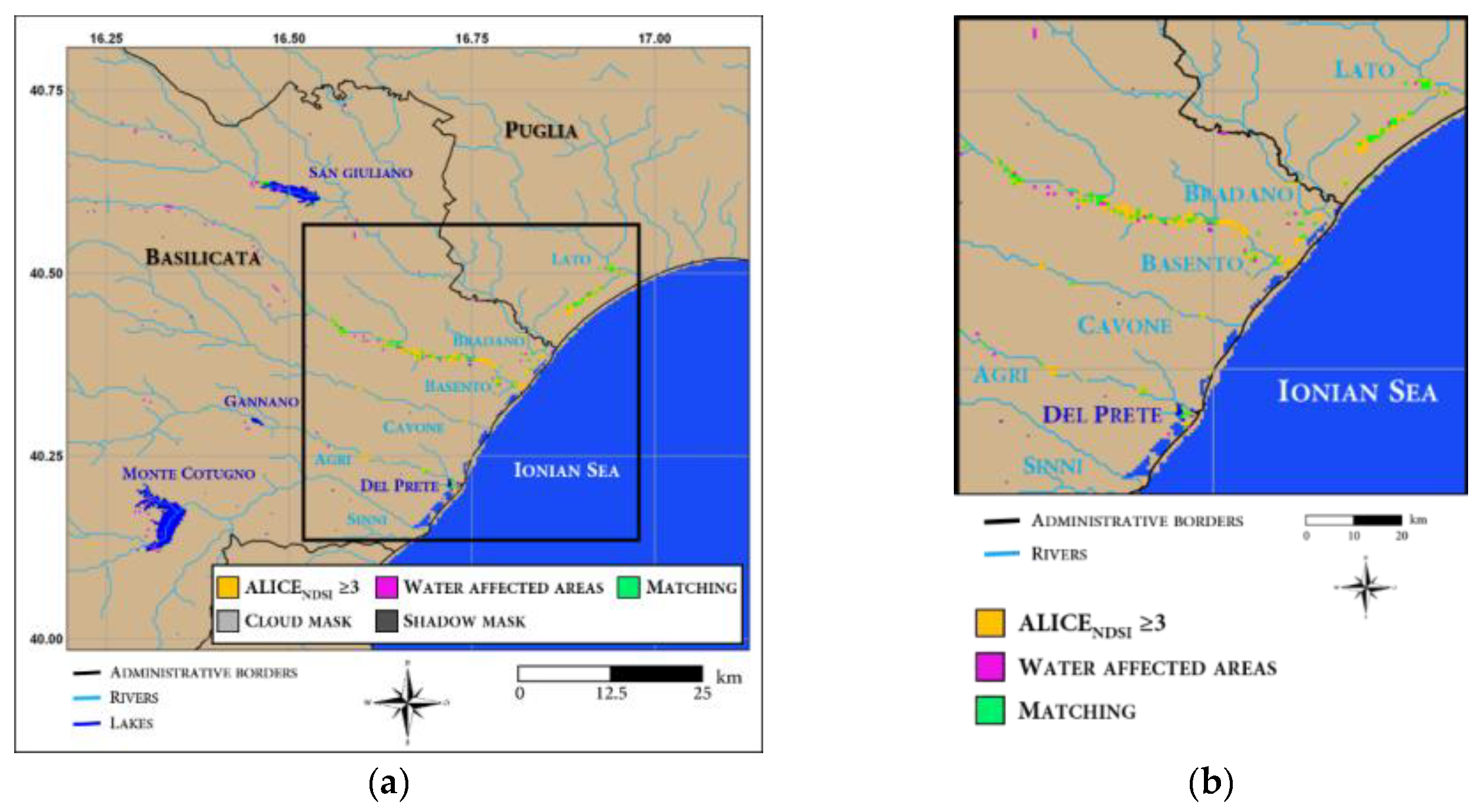
4.3.2. Comparison with the Flood Risk Map
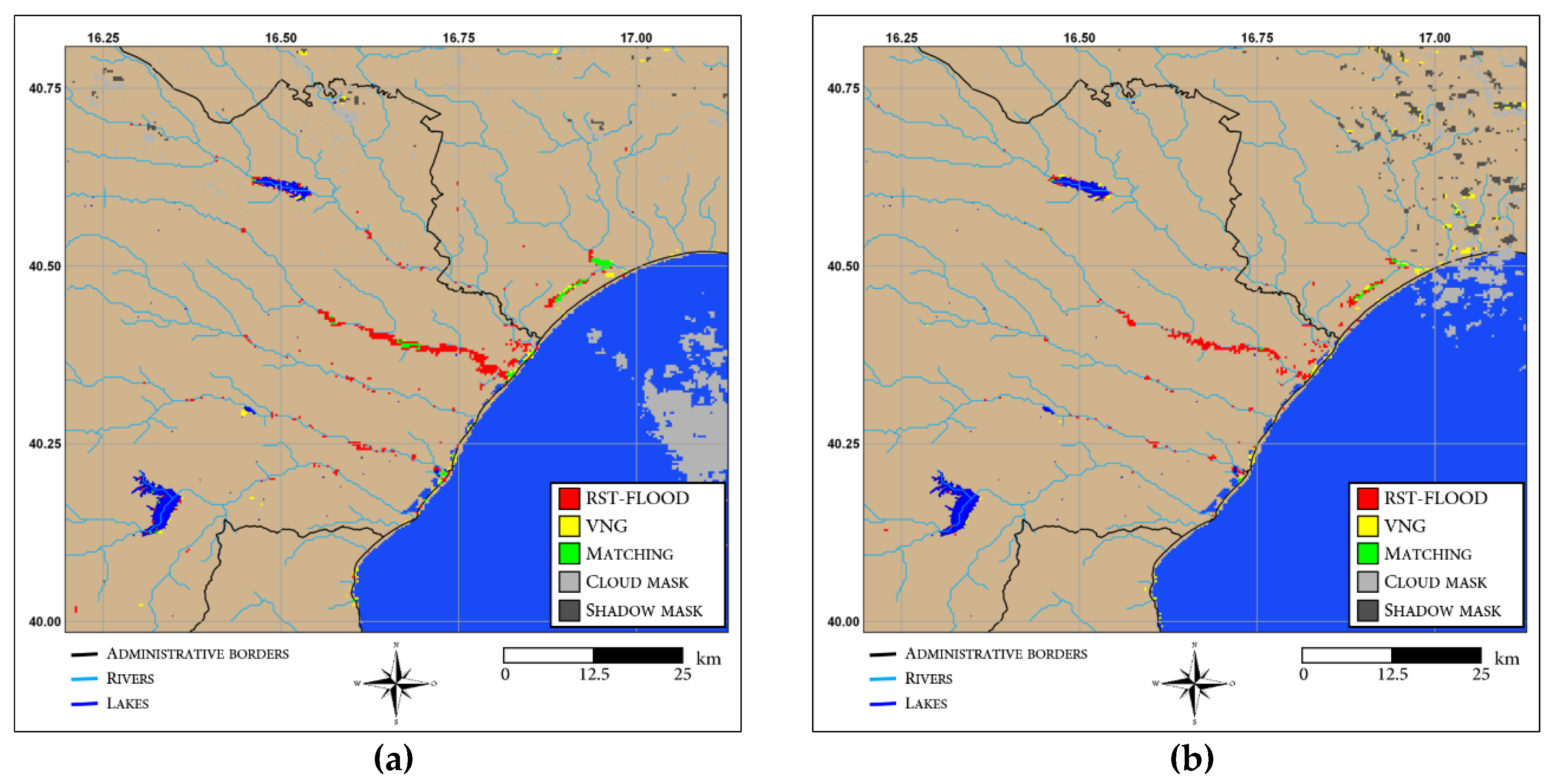
4.3.3. Comparison with VNG
5. Discussion
6. Conclusions
Author Contributions
Funding
Acknowledgments
Conflicts of Interest
References
- Samela, C.; Albano, R.; Sole, A.; Manfreda, S. A GIS tool for cost-effective delineation of flood-prone areas. Comput. Environ. Urban Syst. 2018, 70, 43–52. [Google Scholar] [CrossRef]
- Ward, P.J.; de Perez, E.C.; Dottori, F.; Jongman, B.; Luo, T.; Safaie, S.; Uhlemann-Elmer, S. The Need for Mapping, Modeling, and Predicting Flood Hazard and Risk at the Global Scale. In Global Flood Hazard: Applications in Modeling, Mapping, and Forecasting, 1st ed.; Schumann, G.J.-P., Bates, P.D., Apel, H., Aronica, G.T., Eds.; John Wiley & Sons, Inc.: Hoboken, NJ, USA, 2018; ISBN 978-1-119-21786-2. [Google Scholar]
- Munich, R.E. Topics Geo—Natural Catastrophes 2017. Analyses, Assessments, Positions. 2018. Available online: https://www.munichre.com/site/touch-publications/get/documents_E711248208/mr/assetpool.shared/Documents/5_Touch/_Publications/TOPICS_GEO_2017-en.pdf (accessed on 12 February 2019).
- Antonioli, F.; Anzidei, M.; Amorosi, A.; Presti, V.L.; Mastronuzzi, G.; Deiana, G.; Marsico, A. Sea-level rise and potential drowning of the Italian coastal plains: Flooding risk scenarios for 2100. Quat. Sci. Rev. 2017, 158, 29–43. [Google Scholar] [CrossRef]
- Ward, P.J.; Jongman, B.; Aerts, J.C.J.H.; Bates, P.D.; Botzen, W.J.W.; Diaz, L.A.; Hallegatte, S.; Kind, J.M.; Kwadijk, J.; Scussolini, P.; et al. A global framework for future costs and benefits of river-flood protection in urban areas. Nat. Clim. Chang. 2017, 7, 642–646. [Google Scholar] [CrossRef] [Green Version]
- Sun, D.; Li, S.; Zheng, W.; Croitoru, A.; Stefanidis, A.; Goldberg, M. Mapping floods due to Hurricane Sandy using NPP VIIRS and ATMS data and geotagged Flickr imagery. Int. J. Digit. Earth 2016, 9, 427–441. [Google Scholar] [CrossRef]
- Huang, C.; Chen, Y.; Zhang, S.; Wu, J. Detecting, extracting, and monitoring surface water from space using optical sensors: A review. Rev. Geophys. 2018, 56, 333–360. [Google Scholar] [CrossRef]
- Schumann, G.P.; Brakenridge, G.R.; Kettner, A.J.; Kashif, R.; Niebuhr, E. Assisting Flood Disaster Response with Earth Observation Data and Products: A Critical Assessment. Remote Sens. 2018, 10, 1230. [Google Scholar] [CrossRef]
- Markert, K.L.; Chishtie, F.; Anderson, E.R.; Saah, D.; Griffin, R.E. On the merging of optical and SAR satellite imagery for surface water mapping applications. Results Phys. 2018, 9, 275–277. [Google Scholar] [CrossRef]
- Dasgupta, A.; Grimaldi, S.; Ramsankaran, R.; Pauwels, V.R.N.; Walker, J.P.; Chini, M.; Hostache, R.; Matgen, P. Flood Mapping Using Synthetic Aperture Radar Sensors from Local to Global Scales. In Global Flood Hazard: Applications in Modeling, Mapping, and Forecasting, Geophysical Monograph 233, 1st ed.; John Wiley & Sons, Inc.: Hoboken, NJ, USA, 2018; ISBN 978-1-119-21786-2. [Google Scholar]
- Li, S.; Sun, D.; Goldberg, M.D.; Sjoberg, B.; Santek, D.; Hoffman, J.P.; DeWeese, M.; Restrepo, P.; Lindsey, S.; Holloway, E. Automatic near real-time flood detection using Suomi-NPP/VIIRS data. Remote Sens. Environ. 2018, 204, 672–689. [Google Scholar] [CrossRef]
- The International Charter Space and Major Disasters. Available online: https://disasterscharter.org/web/guest/home (accessed on 12 February 2019).
- Copernicus Emergency Management Service. Available online: https://emergency.copernicus.eu/ (accessed on 12 February 2019).
- Lacava, T.; Ciancia, E.; Faruolo, M.; Pergola, N.; Satriano, V.; Tramutoli, V. Analyzing the December 2013 Metaponto Plain (Southern Italy) Flood Event by Integrating Optical Sensors Satellite Data. Hydrology 2018, 5, 43. [Google Scholar] [CrossRef]
- Fayne, J.; Bolten, J.; Lakshmi, V.; Ahamed, A. Optical and Physical Methods for Mapping Flooding with Satellite Imagery. In Remote Sensing of Hydrological Extremes; Springer Remote Sensing/Photogrammetry; Lakshmi, V., Ed.; Springer International Publishing: Basel, Switzerland, 2017; Chapter 5; pp. 83–103. [Google Scholar] [CrossRef]
- Kwak, Y. Nationwide Flood Monitoring for Disaster Risk Reduction Using Multiple Satellite Data. ISPRS Int. J. Geo-Inf. 2017, 6, 203. [Google Scholar] [CrossRef]
- Ogilvie, A.; Belaud, G.; Massuel, S.; Mulligan, M.; Le Goulven, P.; Calvez, R. Surface water monitoring in small water bodies: Potential and limits of multi-sensor Landsat time series. Hydrol. Earth Syst. Sci. 2018, 22, 4349–4380. [Google Scholar] [CrossRef]
- Lacava, T.; Ciancia, E.; Coviello, I.; Di Polito, C.; Faruolo, M.; Pergola, N.; Satriano, V.; Tramutoli, V. A Satellite Multi-Sensor Approach For Flooded Areas Detection and Monitoring. Adv. Watershed Hydrol. 2015, 51, 83–96. [Google Scholar]
- Brakenridge, G.R. Flood Risk Mapping from Orbital Remote Sensing. In Global Flood Hazard: Applications in Modeling, Mapping, and Forecasting, 1st ed.; Schumann, G.J.-P., Bates, P.D., Apel, H., Aronica, G.T., Eds.; John Wiley & Sons, Inc.: Hoboken, NJ, USA, 2018; ISBN 978-1-119-21786-2. [Google Scholar]
- Normandin, C.; Frappart, F.; Lubac, B.; Bélanger, S.; Marieu, V.; Blarel, F.; Robinet, A.; Guiastrennec-Faugas, L. Quantification of surface water volume changes in the Mackenzie Delta using satellite multi-mission data. Hydrol. Earth Syst. Sci. 2018, 22, 1543–1561. [Google Scholar] [CrossRef] [Green Version]
- Tramutoli, V. Robust Satellite Techniques (RST) for Natural and Environmental Hazards Monitoring and Mitigation: Theory and Applications. In Proceedings of the Fourth International Workshop on the Analysis of Multitemporal Remote Sensing Images, Louven, Belgium, 18–20 July 2007. [Google Scholar] [CrossRef]
- Lacava, T.; Filizzola, C.; Pergola, N.; Sannazzaro, F.; Tramutoli, V. Improving flood monitoring by the Robust AVHRR Technique (RAT) approach: The case of the April 2000 Hungary flood. Int. J. Remote Sens. 2010, 31, 2043–2062. [Google Scholar] [CrossRef]
- Faruolo, M.; Coviello, I.; Lacava, T.; Pergola, N.; Tramutoli, V. A multi-sensor exportable approach for automatic flooded areas detection and monitoring by a composite satellite constellation. IEEE Trans. Geosci. Remote Sens. 2013, 51, 2136–2149. [Google Scholar] [CrossRef]
- Imbrenda, V.; D’Emilio, M.; Lanfredi, M.; Macchiato, M.; Ragosta, M.; Simoniello, T. Indicators for the estimation of vulnerability to land degradation derived from soil compaction and vegetation cover. Eur. J. Soil Sci. 2014, 65, 907–923. [Google Scholar] [CrossRef]
- Imbrenda, V.; Coluzzi, R.; Lanfredi, M.; Loperte, A.; Satriani, A.; Simoniello, T. Analysis of landscape evolution in a vulnerable coastal area under natural and human pressure. Geomat. Nat. Hazards Risk 2018. [Google Scholar] [CrossRef]
- Autorità di Bacino della Basilicata. Mappe della Pericolosità e Mappe del Rischio Idraulico, Relazione 2014. Available online: http://www.adb.basilicata.it/adb/Pstralcio/pianoacque/Relazione_ottobre_2014.pdf (accessed on 12 February 2019).
- Autorità di Bacino della Basilicata. Capitolo IV, Disponibilità: Le Acque superficiali. 2016. Available online: http://www.adb.basilicata.it/adb/pstralcio/bilancioidrico/cap4.pdf (accessed on 12 February 2019).
- Centro Funzionale Decentrato della Protezione Civile Basilicata. Dati in Tempo Reale—Pluviometria. 2018. Available online: http://centrofunzionalebasilicata.it/it/sensoriTempoReale.php?st=I (accessed on 12 February 2019).
- Dal Sasso, S.F.; Cantisani, A.; Lanorte, V.; Pacifico, G.; Manfreda, S. Gli eventi storici della Basilicata. In Le Precipitazioni Estreme in Basilicata, 1st ed.; Manfreda, S., Sole, A., De Costanzo, G., Eds.; Universosud Società Cooperativa: Potenza, Italy, 2015; pp. 6–24. ISBN 978-88-99432-03-4. Available online: http://www.centrofunzionalebasilicata.it/it/pdf/pioggia_download.pdf (accessed on 12 February 2019).
- Di Polito, C.; Ciancia, E.; Coviello, I.; Doxaran, D.; Lacava, T.; Pergola, N.; Satriano, V.; Tramutoli, V. On the Potential of Robust Satellite Techniques Approach for SPM Monitoring in Coastal Waters: Implementation and Application over the Basilicata Ionian Coastal Waters Using MODIS-Aqua. Remote Sens. 2016, 8, 922. [Google Scholar] [CrossRef]
- D’Addabbo, A.; Refice, A.; Pasquariello, G.; Lovergine, F.P.; Capolongo, D.; Manfreda, S. A Bayesian network for flood detection combining SAR imagery and ancillary data. IEEE Trans. Geosci. Remote Sens. 2016, 54, 3612–3625. [Google Scholar] [CrossRef]
- Centro Funzionale Decentrato della Protezione Civile Basilicata. Eventi Metereologici Eccezionali dei Giorni 1, 2 e 3 Dicembre 2013 nel territorio della Regione Basilicata. 2013. Available online: http://www.centrofunzionalebasilicata.it/ew/ew_pdf/r/Report%20evento%20dicembre%202013.pdf (accessed on 12 February 2019).
- Autorità di Bacino della Puglia. Valutazione Globale Provvisoria del Piano di Gestione del Rischio di Alluvioni. 2015. Available online: http://www.adb.puglia.it/public/files/downloads/20151104_PGRA/VGP.pdf (accessed on 12 February 2019).
- Centro Funzionale Decentrato della Protezione Civile Puglia. Rapporto D’evento: Evento Meteo-Idropluviometrico del 30 Novembre–3 Dicembre 2013. 2014. Available online: http://www.protezionecivile.puglia.it/archives/2244 (accessed on 12 February 2019).
- Il Giornale della Protezione Civile Rassegna Stampa del 4/12/2013. 2013. Available online: https://www.ilgiornaledellaprotezionecivile.it/html/download.html?id=7315738794M (accessed on 12 February 2019).
- MeteoWeb. Maltempo, Esonda il Fiume Lato nel Tarantino: Case in Pericolo a Castellaneta Marina. 2013. Available online: http://www.meteoweb.eu/2013/12/maltempo-esonda-il-fiume-lato-nel-tarantino-case-in-pericolo-a-castellaneta-marina/244468/#LL1PsEgcYY9bjUwO.99 (accessed on 12 February 2019).
- De Musso, N.M.; Capolongo, D.; Refice, A.; Lovergine, F.P.; D’Addabbo, A.; Pennetta, L. Spatial evolution of the December 2013 Metaponto plain (Basilicata, Italy) flood event using multi-source and high-resolution remotely sensed data. J. Maps 2018, 14, 219–229. [Google Scholar] [CrossRef]
- Joint Polar Satellite System (JPSS). JPSS-1 has a New Name: NOAA-20. 2017. Available online: http://www.jpss.noaa.gov/launch.html (accessed on 12 February 2019).
- National Environmental Satellite, Data, and Information Service (NESDIS). Polar Satellite Programs Continuity of Weather Observations. 2018. Available online: https://www.nesdis.noaa.gov/sites/default/files/asset/document/Polar_Flyout%20Jan_2018_Weather_Signed_Linked.pdf (accessed on 12 February 2019).
- Cao, C.; Xiong, J.; Blonski, S.; Liu, Q.; Uprety, S.; Shao, X.; Bai, Y.; Weng, F. Suomi NPP VIIRS sensor data record verification, validation, and long-term performance monitoring. J. Geophys. Res. Atmos. 2013, 118, 664–678. [Google Scholar] [CrossRef]
- NOAA Comprehensive Large Array-data Stewardship System (CLASS). 2019. Available online: https://www.avl.class.noaa.gov/saa/products/welcome (accessed on 12 February 2019).
- Polar2Grid, 2018. Available online: https://www.ssec.wisc.edu/software/polar2grid/# (accessed on 12 February 2019).
- Geoportale Nazionale—Ministero dell’Ambiente e della Tutela del Territorio e del Mare. 2018. Available online: http://www.pcn.minambiente.it/mattm/direttiva-alluvioni/ (accessed on 12 February 2019).
- Community Satellite Processing Package (CSPP). Suomi-NPP VIIRS Flood Detection Software Version 1.0 Release. 2018. Available online: http://cimss.ssec.wisc.edu/cspp/viirs_flood_v1.0.shtml (accessed on 12 February 2019).
- USGS Earth Explorer. Available online: https://earthexplorer.usgs.gov/ (accessed on 12 February 2019).
- Quinn, J.W. Landsat Band Combination. Available online: http://web.pdx.edu/~emch/ip1/bandcombinations.html (accessed on 12 February 2019).
- USGS Landsat Missions. Available online: https://landsat.usgs.gov/known-issues (accessed on 12 February 2019).
- Sole, A.; Giosa, L.; Copertino, V. Risk flood areas, a case study: Basilicata Region. WIT Trans. Ecol. Environ. 2017, 104, 213–228. Available online: https://www.witpress.com/Secure/elibrary/papers/RM07/RM07021FU1.pdf (accessed on 12 February 2019). [CrossRef]
- Tramutoli, V. Robust AVHRR Techniques (RAT) for Environmental Monitoring: Theory and applications. Earth Surface Remote Sensing II, Giovanna Cecchi, Eugenio Zilioli, Editors. Proc. SPIE 1998, 3496, 101–113. [Google Scholar]
- Ciancia, E.; Coviello, I.; Di Polito, C.; Lacava, T.; Pergola, N.; Satriano, V.; Tramutoli, V. Investigating the chlorophyll-a variability in the Gulf of Taranto (North-western Ionian Sea) by a multi-temporal analysis of MODIS-Aqua Level 3/Level 2 data. Cont. Shelf Res. 2018, 155, 34–44. [Google Scholar] [CrossRef]
- Koeppen, W.C.; Pilger, E.; Wright, R. Time series analysis of infrared satellite data for detecting thermal anomalies: A hybrid approach. Bull. Volcanol. 2011, 73, 577–593. [Google Scholar] [CrossRef]
- Cuomo, V.; Filizzola, C.; Pergola, N.; Pietrapertosa, C.; Tramutoli, V. A self-sufficient approach for GERB cloudy radiance detection. Atmos. Res. 2004, 72, 39–56. [Google Scholar] [CrossRef]
- Pietrapertosa, C.; Pergola, N.; Lanorte, V.; Tramutoli, V. Self Adaptive Algorithms for Change Detection: OCA (the One-channel Cloud-detection Approach) an adjustable method for cloudy and clear radiances detection. In Proceedings of the Technical Proceedings of the Eleventh International (A)TOVS Study Conference (ITSC-XI), Budapest, Hungary, 20–26 September 2000; pp. 281–291. [Google Scholar]
- Huang, C.; Chen, Y.; Wu, J.; Li, L.; Liu, R. An evaluation of Suomi NPP-VIIRS data for surface water detection. Remote Sens. Lett. 2015, 6, 155–164. [Google Scholar] [CrossRef]
- Xiao, X.G.; Shen, Z.X.; Qin, X.G. Assessing the potential of vegetation sensor data for mapping snow and ice cover: A Normalized Difference Snow and Ice Index. Int. J. Remote Sens. 2001, 22, 2479–2487. [Google Scholar] [CrossRef]
- Boschetti, M.; Nutini, F.; Manfron, G.; Brivio, P.A.; Nelson, A. Comparative Analysis of Normalised Difference Spectral Indices Derived from MODIS for Detecting Surface Water in Flooded Rice Cropping Systems. PLoS ONE 2014, 9, e88741. [Google Scholar] [CrossRef]
- Piper, M.; Bahr, T. A rapid cloud mask algorithm for SUOMI NPP VIIRS imagery EDRS. The International Archives of the Photogrammetry, Remote Sensing and Spatial Information Sciences. In Proceedings of the 36th International Symposium on Remote Sensing of Environment, Berlin, Germany, 11–15 May 2015; Volume XL-7/W3. [Google Scholar]
- Candra, D.S.; Phinn, S.; Scarth, P. Cloud and cloud shadow masking using multi-temporal cloud masking algorithm in tropical environmental. The International Archives of the Photogrammetry, Remote Sensing and Spatial Information Sciences. In Proceedings of the XXIII ISPRS Congress, Prague, Czech Republic, 12–19 July 2016; Volume XLI-B2. [Google Scholar] [CrossRef]
- Zhu, Z.; Woodcock, C.E. Object-based cloud and cloud shadow detection in Landsat imagery. Remote Sens. Environ. 2012, 118, 83–94. [Google Scholar] [CrossRef]
- Sanyal, J.; Lu, X.X. Application of Remote Sensing in Flood Management with Special Reference to Monsoon Asia: A Review. Nat. Hazards 2014, 33, 283–301. [Google Scholar] [CrossRef]
- Franci, F.; Mandanici, E.; Bitelli, G. Remote sensing analysis for flood risk management in urban sprawl contexts. Geomat. Nat. Hazards Risk 2015, 6, 583–599. [Google Scholar] [CrossRef]
- Lacava, T.; Brocca, L.; Coviello, I.; Faruolo, M.; Pergola, N.; Tramutoli, V. Integration of optical and passive microwave satellite data for flooded area detection and monitoring. In Engineering Geology for Society and Territory; Springer International Publishing: Basel, Switzerland, 2014; Volume 3, pp. 631–635. [Google Scholar] [CrossRef]
- Tramutoli, V.; Claps, P.; Marella, M.; Pergola, N.; Sileo, C. Feasibility of hydrological application of thermal inertia from remote sensing. In Proceedings of the 2nd Plinius Conference on Mediterranean Storms, Siena, Italy, 16–18 October 2000; pp. 16–18. [Google Scholar]
- Verstraeten, W.W.; Veroustraete, F.; van der Sande, C.J.; Grootaers, I.; Feyen, J. Soil moisture retrieval using thermal inertia, determined with visible and thermal spaceborne data validated for European forests. Remote Sens. Environ. 2006, 101, 299–314. [Google Scholar] [CrossRef]
- Piccarreta, M.; Pasini, A.; Capolongo, D.; Lazzari, M. Changes in daily precipitation extremes in the Mediterranean from 1951 to 2010: The Basilicata region, Southern Italy. Int. J. Climatol. 2013, 33, 3229–3248. [Google Scholar] [CrossRef]


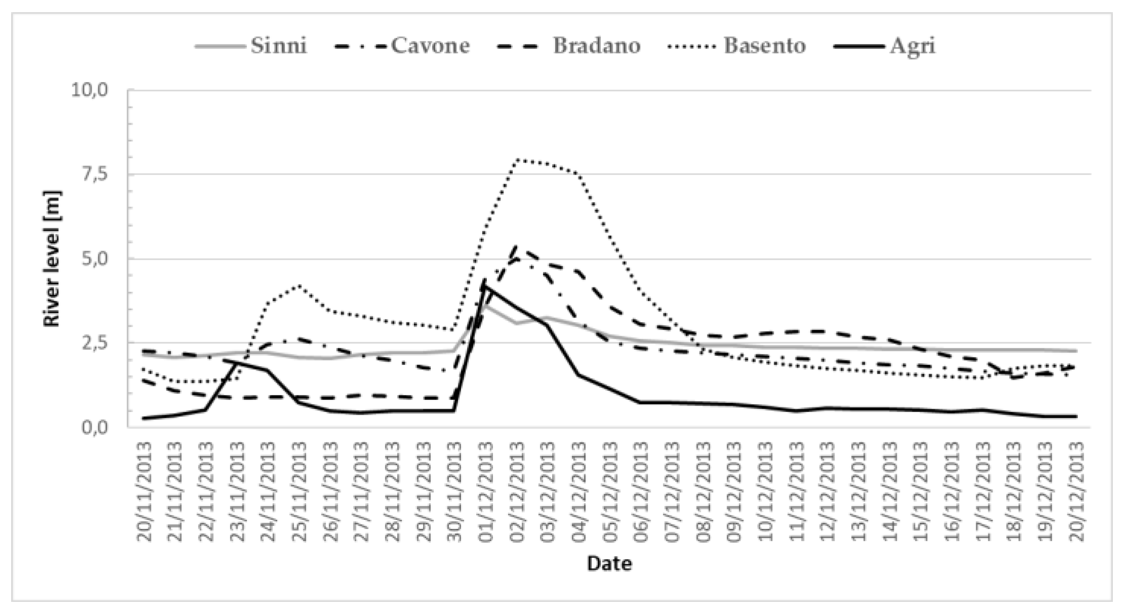
| Sinni | Agri | Cavone | Basento | Bradano | |
|---|---|---|---|---|---|
| Max River Level Date | 3.59 m 01/12/2013 | 4.19 m 01/12/2013 | 5.22 m 04/02/2014 | 7.92 m 02/12/2013 | 6.04 m 02/03/2011 |
| 3.47 m 28/03/2015 | 3.93 m 13/03/2016 | 5.00 m 02/12/2013 | 7.81 m 03/12/2013 | 5.39 m 02/12/2013 | |
| 3.46 m 23/02/2012 | 3.55 m 02/12/2013 | 4.81 m 19/02/2011 | 7.60 m 02/03/2011 | 4.83 m 03/12/2013 |
| ALICE Index | All Scene | Basento River | ||||
|---|---|---|---|---|---|---|
| # Anomalous Pixels | Mean | Max/Min | # Anomalous Pixels | Mean | Max/Min | |
| ALICESWIR | 220 | −2.42 | −28.16 | 71 | −3.98 | −7.48 |
| ALICERED-SWIR | 604 | 4.70 | 17.15 | 230 | 6.28 | 17.15 |
| ALICERED/SWIR | 679 | 8.92 | 61.83 | 247 | 3.06 | 61.83 |
| ALICENDSI | 638 | 5.78 | 23.74 | 256 | 3.01 | 23.74 |
| All scene | Black Box | |||
|---|---|---|---|---|
| Pixels Number | % | Pixels Number | % | |
| included in PAI area | 617 | 68% | 537 | 76% |
| not included in PAI area | 295 | 32% | 172 | 24% |
| All Scene Pixels Number | Black Box Pixels Number | |||||
|---|---|---|---|---|---|---|
| VIIRS Data | RST-FLOOD | VNG | MATCHING | RST-FLOOD | VNG | MATCHING |
| 04/12/2013 | 638 | 454 | 109 | 510 | 184 | 96 |
| 05/12/2013 | 357 | 481 | 36 | 293 | 111 | 31 |
| 06/12/2013 | 267 | 234 | 26 | 226 | 84 | 18 |
| 07/12/2013 | 345 | 196 | 4 | 317 | 71 | 4 |
| 08/12/2013 | 260 | 137 | 3 | 211 | 10 | 0 |
© 2019 by the authors. Licensee MDPI, Basel, Switzerland. This article is an open access article distributed under the terms and conditions of the Creative Commons Attribution (CC BY) license (http://creativecommons.org/licenses/by/4.0/).
Share and Cite
Lacava, T.; Ciancia, E.; Faruolo, M.; Pergola, N.; Satriano, V.; Tramutoli, V. On the Potential of RST-FLOOD on Visible Infrared Imaging Radiometer Suite Data for Flooded Areas Detection. Remote Sens. 2019, 11, 598. https://0-doi-org.brum.beds.ac.uk/10.3390/rs11050598
Lacava T, Ciancia E, Faruolo M, Pergola N, Satriano V, Tramutoli V. On the Potential of RST-FLOOD on Visible Infrared Imaging Radiometer Suite Data for Flooded Areas Detection. Remote Sensing. 2019; 11(5):598. https://0-doi-org.brum.beds.ac.uk/10.3390/rs11050598
Chicago/Turabian StyleLacava, Teodosio, Emanuele Ciancia, Mariapia Faruolo, Nicola Pergola, Valeria Satriano, and Valerio Tramutoli. 2019. "On the Potential of RST-FLOOD on Visible Infrared Imaging Radiometer Suite Data for Flooded Areas Detection" Remote Sensing 11, no. 5: 598. https://0-doi-org.brum.beds.ac.uk/10.3390/rs11050598