Mapping Agricultural Landuse Patterns from Time Series of Landsat 8 Using Random Forest Based Hierarchial Approach


Abstract
:1. Introduction
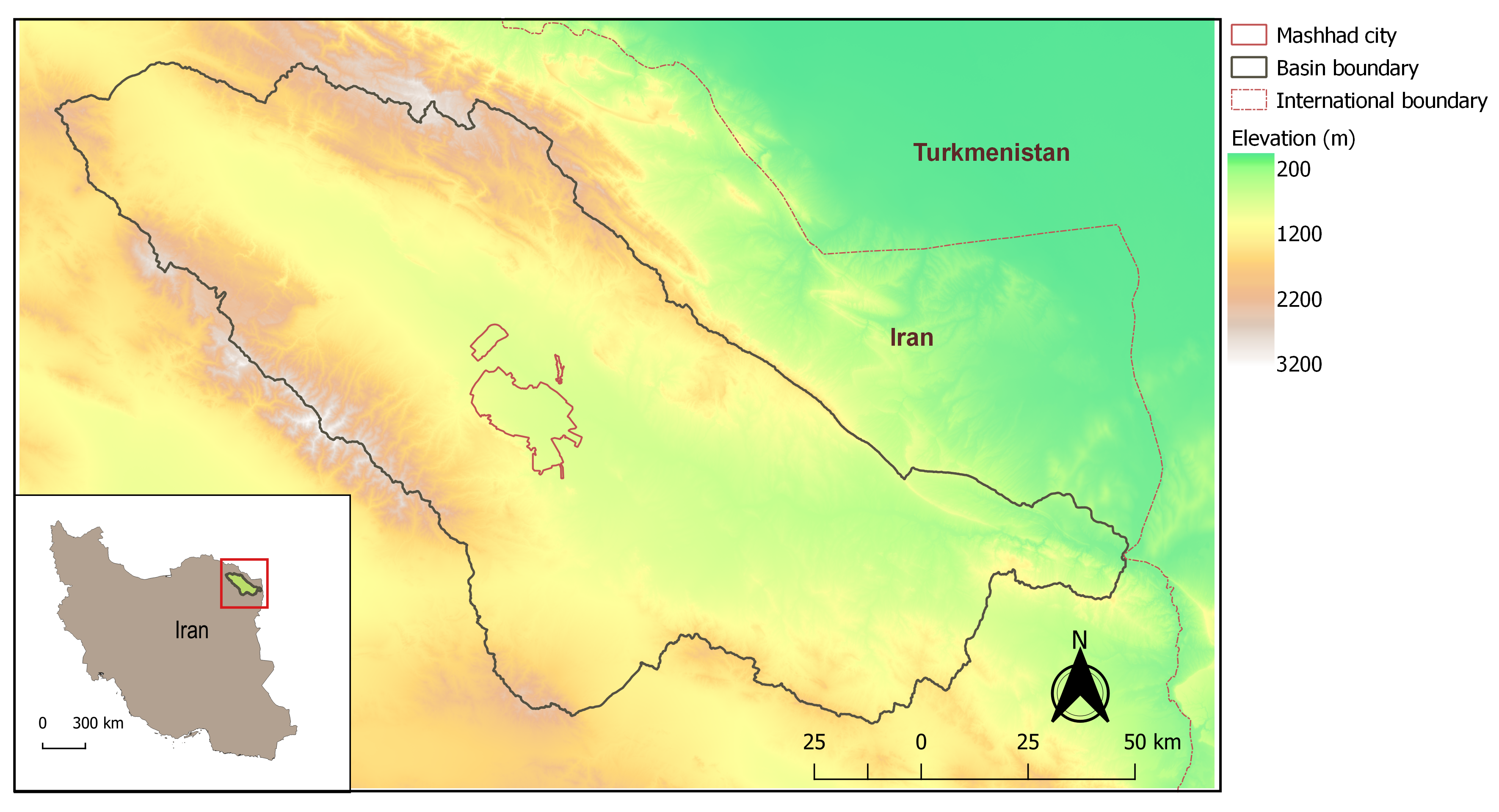
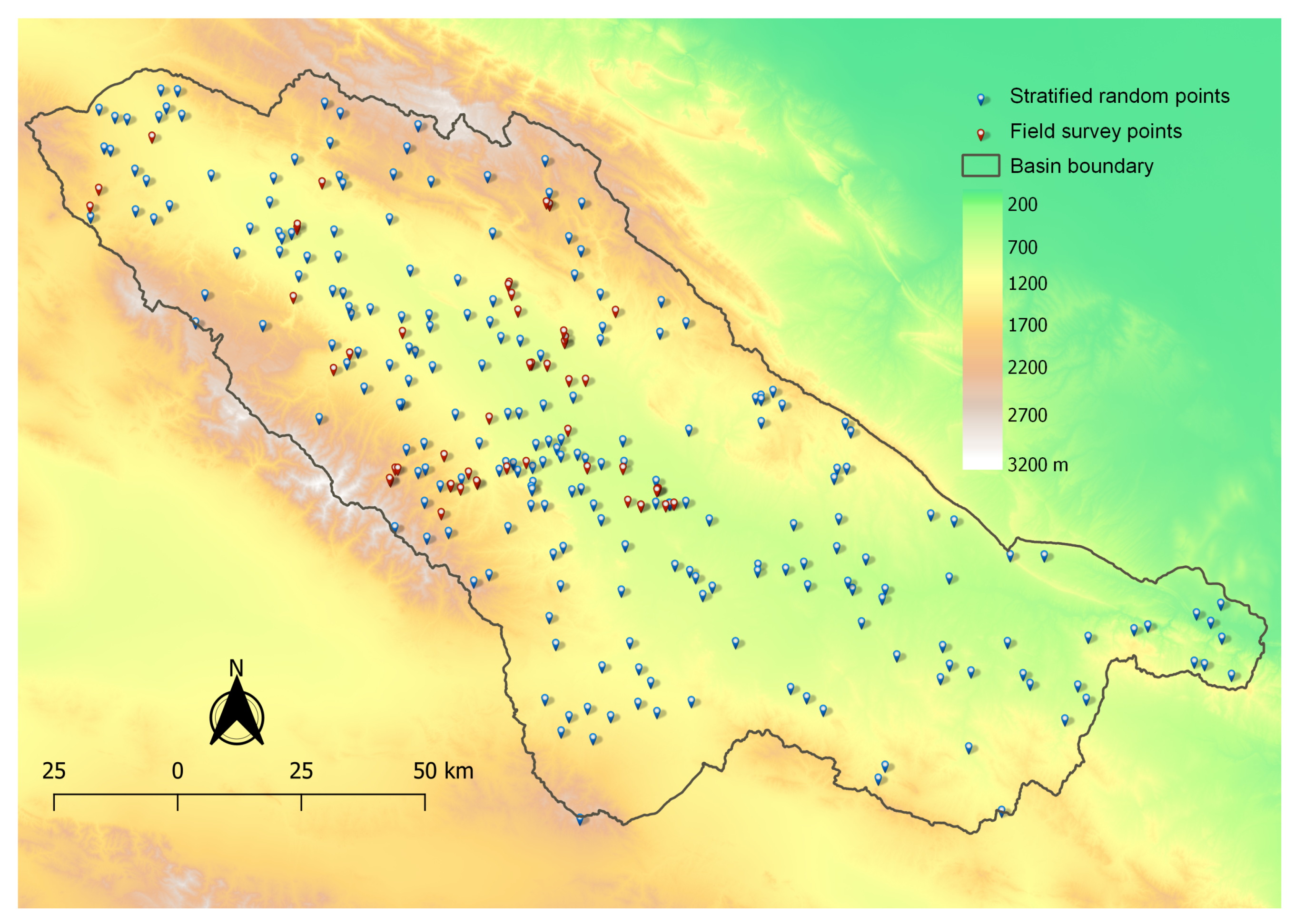
2. Study Area
3. Methods
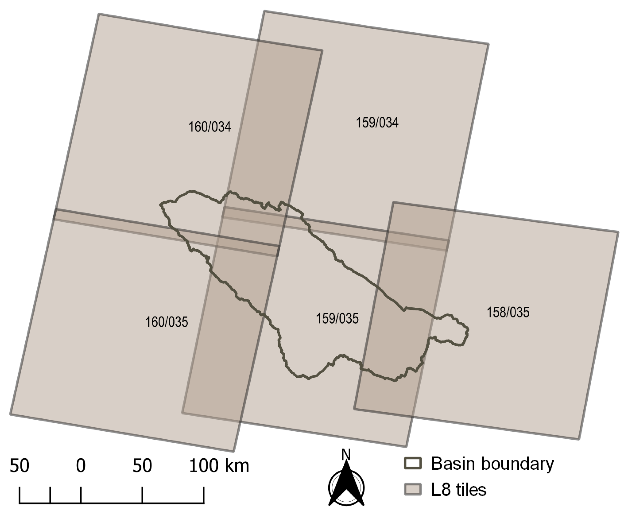
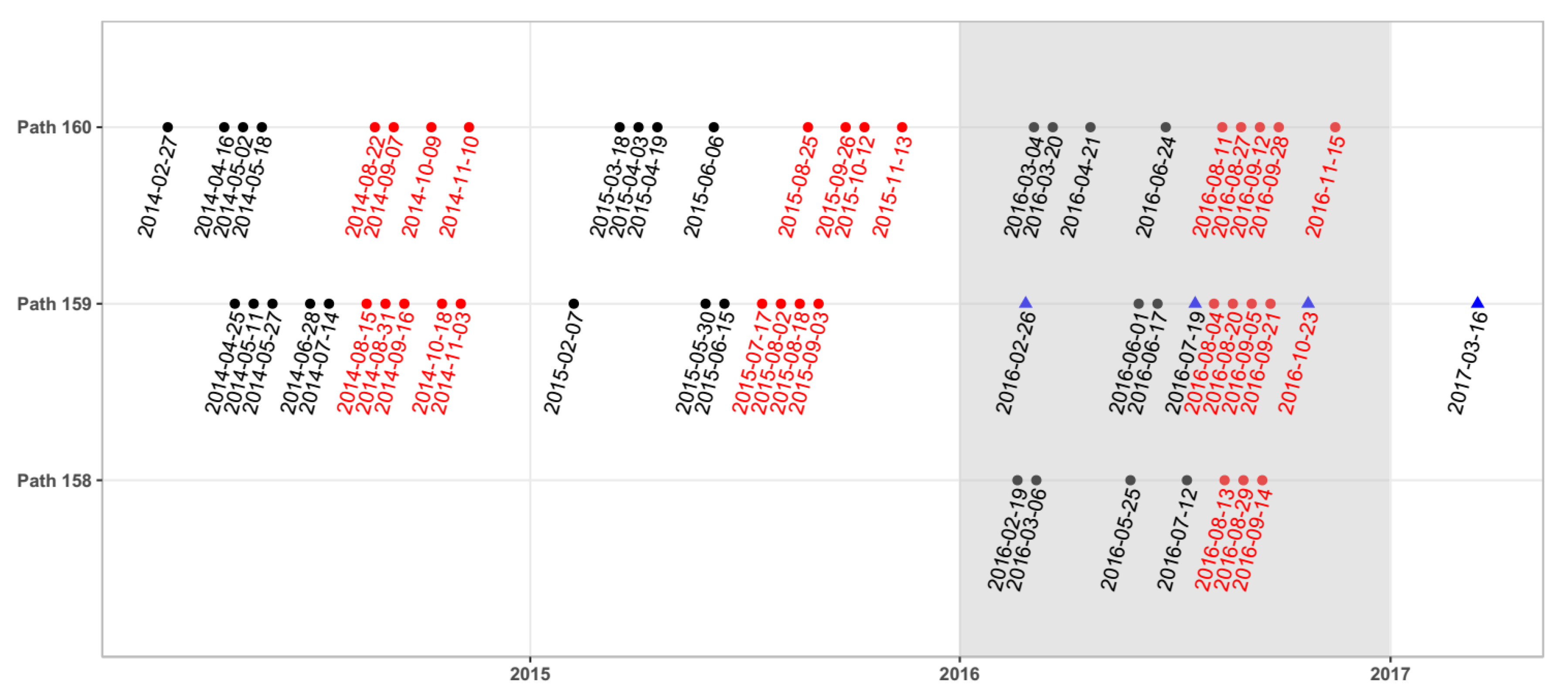
3.1. Satellite Data
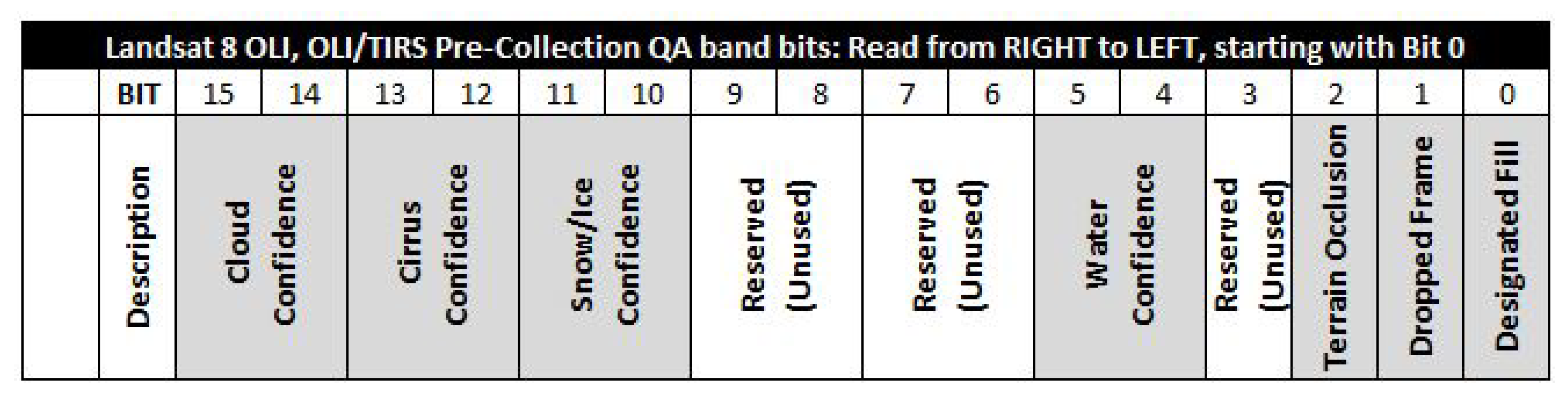
3.2. Pre-Processing Landsat 8 Data
3.3. Training and Validation Samples
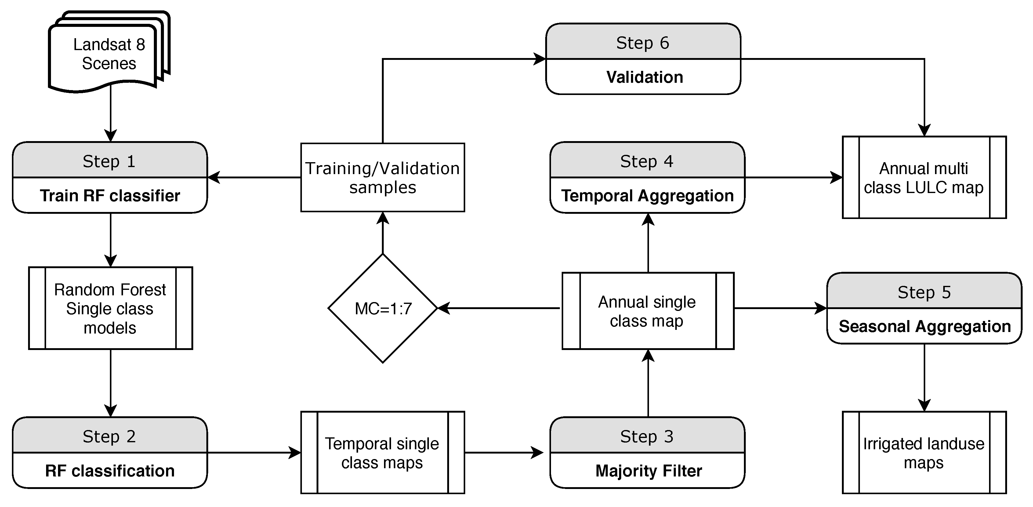
3.4. Classification Using Random Forest (RF)
- Developing seven single class RF models from the four candidate L8 data.
- Applying those single class RF models to individual scenes of all the required tiles to extract single class maps for each acquisition and tile.
- Applying majority fusion to aggregate over multiple acquisitions to single class maps for each tile.
- For irrigated area class, applying a single occurrence selection method to aggregate the single class maps for each tile.
- Mosaicking the single class maps for each tile to a single class maps for entire Mashhad basin.
- Conditionally patching all the single class maps for basin to a multi-class LULC map for the year.
- Seasonally aggregating to derive land use types for irrigated area.
4. Results
4.1. Resampling L8 Spectral Bands
4.2. RF Model Performance
4.3. Classification and Accuracy Assessment
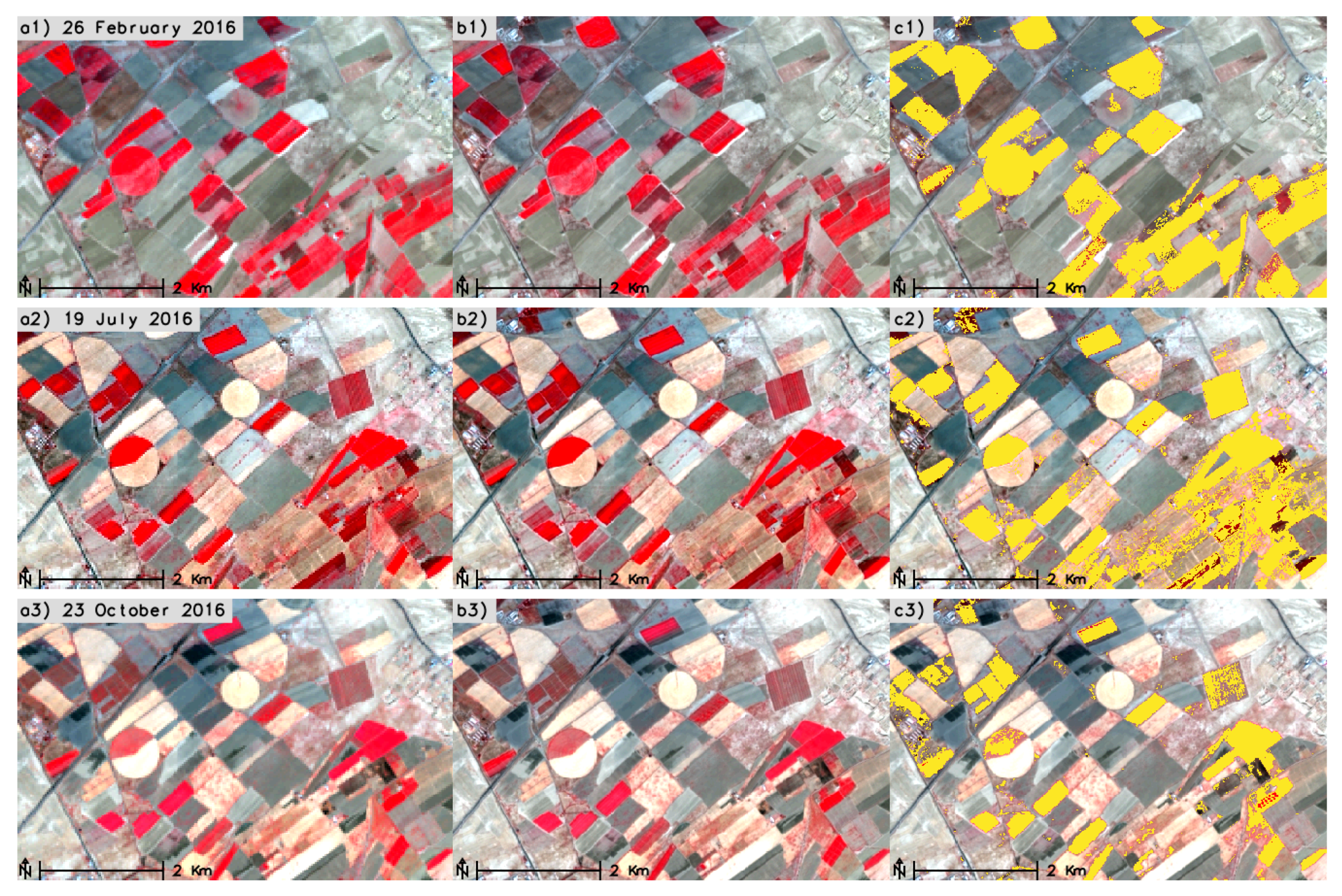
4.4. Spatial and Temporal Crop Patterns
5. Discussion
6. Conclusions
Author Contributions
Funding
Acknowledgments
Conflicts of Interest
References
- Rijsberman, F.R. Water scarcity: Fact or fiction? Agric. Water Manag. 2006, 80, 5–22. [Google Scholar] [CrossRef]
- Gosling, S.N.; Arnell, N.W. A global assessment of the impact of climate change on water scarcity. Clim. Chang. 2016, 134, 371–385. [Google Scholar] [CrossRef]
- Vörösmarty, C.J.; Green, P.; Salisbury, J.; Lammers, R.B. Global Water Resources: Vulnerability from Climate Change and Population Growth. Science 2000, 289, 284–288. [Google Scholar] [CrossRef] [PubMed]
- Mukherji, A.; Facon, T.; de Fraiture, C.; Molden, D.; Chartres, C. Growing more food with less water: How can revitalizing Asia’s irrigation help? Water Policy 2012, 14, 430–446. [Google Scholar] [CrossRef]
- Seckler, D.; Barker, R.; Amarasinghe, U. Water Scarcity in the Twenty-first Century. Int. J. Water Resour. Dev. 1999, 15, 29–42. [Google Scholar] [CrossRef]
- Cosgrove, W.J.; Rijsberman, F.R. World Water Vision: Making Water Everybody’s Business; Earthscan Publications: London, UK, 2000. [Google Scholar]
- Karimi, P.; Molden, D.; Notenbaert, A.; Peden, D. Nile basin farming systems and productivity. In The Nile River Basin; Water, Agriculture, Governance and Livelihoods; Routledge: Abingdon, UK, 2012; pp. 133–153. [Google Scholar]
- United Nations (UN). General Assembly, Transforming Our World: The 2030 Agenda for Sustainable Development; Resolution Adopted by the United Nations General Assembly on 25 September 2015; United Nations: New York, NY, USA, 2015. [Google Scholar]
- Levidow, L.; Zaccaria, D.; Maia, R.; Vivas, E.; Todorovic, M.; Scardigno, A. Improving water-efficient irrigation: Prospects and difficulties of innovative practices. Agric. Water Manag. 2014, 146, 84–94. [Google Scholar] [CrossRef]
- Ozdogan, M.; Yang, Y.; Allez, G.; Cervantes, C. Remote Sensing of Irrigated Agriculture: Opportunities and Challenges. Remote Sens. 2010, 2, 2274–2304. [Google Scholar] [CrossRef]
- Grafton, R.Q.; Williams, J.; Perry, C.J.; Molle, F.; Ringler, C.; Steduto, P.; Udall, B.; Wheeler, S.A.; Wang, Y.; Garrick, D.; et al. The paradox of irrigation efficiency. Science 2018, 361, 748–750. [Google Scholar] [CrossRef]
- Bastiaanssen, W.G.M.; Karimi, P.; Rebelo, L.M.; Duan, Z.; Senay, G.; Muthuwatte, L.; Smakhtin, V. Earth Observation Based Assessment of the Water Production and Water Consumption of Nile Basin Agro-Ecosystems. Remote Sens. 2014, 6, 10306–10334. [Google Scholar] [CrossRef]
- Ajaz, A.; Karimi, P.; de Fraiture, C.; Xueliang, C. National and global censuses or satellite-based estimates? Asia’s irrigated areas: In a muddle. In Proceedings of the 2nd World Irrigation Forum, Chiang Mai, Thailand, 6–8 November 2016. [Google Scholar]
- Bastiaanssen, W.G.M. Remote Sensing in Water Resources Management: The State of the Art; IWMI Research Report; International Water Management Institute: Colombo, Sri Lanka, 1998; p. 118. [Google Scholar]
- Bastiaanssen, W.G.M.; Molden, D.J.; Makin, I.W. Remote sensing for irrigated agriculture: Examples from research and possible applications. Agric. Water Manag. 2000, 46, 137–155. [Google Scholar] [CrossRef]
- Thenkabail, P.S.; Biradar, C.M.; Noojipady, P.; Dheeravath, V.; Li, Y.; Velpuri, M.; Gumma, M.; Gangalakunta, O.R.P.; Turral, H.; Cai, X.; et al. Global irrigated area map (GIAM), derived from remote sensing, for the end of the last millennium. Int. J. Remote Sens. 2009, 30, 3679–3733. [Google Scholar] [CrossRef]
- Biradar, C.M.; Thenkabail, P.S.; Noojipady, P.; Li, Y.; Dheeravath, V.; Turral, H.; Velpuri, M.; Gumma, M.K.; Gangalakunta, O.R.P.; Cai, X.L.; et al. A global map of rainfed cropland areas (GMRCA) at the end of last millennium using remote sensing. Int. J. Appl. Earth Obs. Geoinf. 2009, 11, 114–129. [Google Scholar] [CrossRef]
- Zhang, H.K.; Roy, D.P. Using the 500m MODIS land cover product to derive a consistent continental scale 30m Landsat land cover classification. Remote Sens. Environ. 2017, 197, 15–34. [Google Scholar] [CrossRef]
- Cieślak, I.; Szuniewicz, K.; Pawlewicz, K.; Czyża, S. Land Use Changes Monitoring with CORINE Land Cover Data. IOP Conf. Ser. Mater. Sci. Eng. 2017, 245, 052049. [Google Scholar] [CrossRef]
- Ambika, A.K.; Wardlow, B.; Mishra, V. Remotely sensed high resolution irrigated area mapping in India for 2000 to 2015. Sci. Data 2016, 3, 160118. [Google Scholar] [CrossRef] [PubMed]
- Funk, C.; Verdin, J.P. Real-Time Decision Support Systems: The Famine Early Warning System Network. In Satellite Rainfall Applications for Surface Hydrology; Gebremichael, M., Hossain, F., Eds.; Springer: Dordrecht, The Netherlands, 2010; pp. 295–320. [Google Scholar] [CrossRef]
- López-Lozano, R.; Duveiller, G.; Seguini, L.; Meroni, M.; García-Condado, S.; Hooker, J.; Leo, O.; Baruth, B. Towards regional grain yield forecasting with 1km-resolution EO biophysical products: Strengths and limitations at pan-European level. Agric. For. Meteorol. 2015, 206, 12–32. [Google Scholar] [CrossRef]
- Wu, B.; Meng, J.; Li, Q.; Yan, N.; Du, X.; Zhang, M. Remote sensing-based global crop monitoring: Experiences with China’s CropWatch system. Int. J. Digit. Earth 2014, 7, 113–137. [Google Scholar] [CrossRef]
- Becker-Reshef, I.; Justice, C.; Sullivan, M.; Vermote, E.; Tucker, C.; Anyamba, A.; Small, J.; Pak, E.; Masuoka, E.; Schmaltz, J.; et al. Monitoring Global Croplands with Coarse Resolution Earth Observations: The Global Agriculture Monitoring (GLAM) Project. Remote Sens. 2010, 2, 1589–1609. [Google Scholar] [CrossRef]
- Rembold, F.; Meroni, M.; Urbano, F.; Lemoine, G.; Kerdiles, H.; Perez-Hoyos, A.; Csak, G. ASAP—Anomaly hot Spots of Agricultural Production, a new early warning decision support system developed by the Joint Research Centre. In Proceedings of the 2017 9th International Workshop on the Analysis of Multitemporal Remote Sensing Images (MultiTemp), Brugge, Belgium, 27–29 June 2017; pp. 1–5. [Google Scholar] [CrossRef]
- Fritz, S.; See, L.; Bayas, J.C.L.; Waldner, F.; Jacques, D.; Becker-Reshef, I.; Whitcraft, A.; Baruth, B.; Bonifacio, R.; Crutchfield, J.; et al. A comparison of global agricultural monitoring systems and current gaps. Agric. Syst. 2019, 168, 258–272. [Google Scholar] [CrossRef]
- Atzberger, C. Advances in Remote Sensing of Agriculture: Context Description, Existing Operational Monitoring Systems and Major Information Needs. Remote Sens. 2013, 5, 949–981. [Google Scholar] [CrossRef]
- Jones, J.W.; Antle, J.M.; Basso, B.; Boote, K.J.; Conant, R.T.; Foster, I.; Godfray, H.C.J.; Herrero, M.; Howitt, R.E.; Janssen, S.; et al. Toward a new generation of agricultural system data, models, and knowledge products: State of agricultural systems science. Agric. Syst. 2017, 155, 269–288. [Google Scholar] [CrossRef] [PubMed]
- Gómez, C.; White, J.C.; Wulder, M.A. Optical remotely sensed time series data for land cover classification: A review. ISPRS J. Photogramm. Remote Sens. 2016, 116, 55–72. [Google Scholar] [CrossRef]
- Liu, P. A survey of remote-sensing big data. Environ. Inform. 2015, 3, 45. [Google Scholar] [CrossRef]
- Inglada, J.; Arias, M.; Tardy, B.; Morin, D.; Valero, S.; Hagolle, O.; Dedieu, G.; Sepulcre, G.; Bontemps, S.; Defourny, P. Benchmarking of algorithms for crop type land-cover maps using Sentinel-2 image time series. In Proceedings of the 2015 IEEE International Geoscience and Remote Sensing Symposium (IGARSS), Milan, Italy, 26–31 July 2015; pp. 3993–3996. [Google Scholar] [CrossRef]
- Maxwell, A.E.; Warner, T.A.; Fang, F. Implementation of machine-learning classification in remote sensing: An applied review. Int. J. Remote Sens. 2018, 39, 2784–2817. [Google Scholar] [CrossRef]
- Inglada, J.; Vincent, A.; Arias, M.; Tardy, B.; Morin, D.; Rodes, I. Operational High Resolution Land Cover Map Production at the Country Scale Using Satellite Image Time Series. Remote Sens. 2017, 9, 95. [Google Scholar] [CrossRef]
- Inglada, J.; Arias, M.; Tardy, B.; Hagolle, O.; Valero, S.; Morin, D.; Dedieu, G.; Sepulcre, G.; Bontemps, S.; Defourny, P.; et al. Assessment of an Operational System for Crop Type Map Production Using High Temporal and Spatial Resolution Satellite Optical Imagery. Remote Sens. 2015, 7, 12356–12379. [Google Scholar] [CrossRef]
- Rodriguez-Galiano, V.F.; Ghimire, B.; Rogan, J.; Chica-Olmo, M.; Rigol-Sanchez, J.P. An assessment of the effectiveness of a random forest classifier for land-cover classification. ISPRS J. Photogramm. Remote Sens. 2012, 67, 93–104. [Google Scholar] [CrossRef]
- Berhane, T.M.; Lane, C.R.; Wu, Q.; Autrey, B.C.; Anenkhonov, O.A.; Chepinoga, V.V.; Liu, H. Decision-Tree, Rule-Based, and Random Forest Classification of High-Resolution Multispectral Imagery for Wetland Mapping and Inventory. Remote Sens. 2018, 10, 580. [Google Scholar] [CrossRef]
- Karimi, P.; Molden, D.; Bastiaanssen, W.; Cai, X. Water accounting to assess use and productivity of water: Evolution of a concept and new frontiers. In Water Accounting: International Approaches to Policy and Decision-Making; Edward Elgar Publishing: Cheltenham, UK, 2012; pp. 76–88. [Google Scholar]
- Motagh, M.; Djamour, Y.; Walter, T.R.; Wetzel, H.U.; Zschau, J.; Arabi, S. Land subsidence in Mashhad Valley, northeast Iran: Results from InSAR, levelling and GPS. Geophys. J. Int. 2007, 168, 518–526. [Google Scholar] [CrossRef]
- Karimi, P.; Qureshi, A.S.; Bahramloo, R.; Molden, D. Reducing carbon emissions through improved irrigation and groundwater management: A case study from Iran. Agric. Water Manag. 2012, 108, 52–60. [Google Scholar] [CrossRef]
- Neteler, M.; Bowman, M.H.; Landa, M.; Metz, M. GRASS GIS: A multi-purpose open source GIS. Environ. Model. Softw. 2012, 31, 124–130. [Google Scholar] [CrossRef]
- Grizonnet, M.; Michel, J.; Poughon, V.; Inglada, J.; Savinaud, M.; Cresson, R. Orfeo ToolBox: Open source processing of remote sensing images. Open Geospat. Data Softw. Stand. 2017, 2, 15. [Google Scholar] [CrossRef]
- United States Geological Survey (USGS). Landsat 8 (L8) Data Users Handbook; Department of the Interior U.S. Geological Survey: Sioux Falls, SD, USA, 2016.
- Gangkofner, U.G.; Pradhan, P.S.; Holcomb, D.W. Optimizing the High-Pass Filter Addition Technique for Image Fusion. Photogramm. Eng. Remote Sens. 2007, 73, 1107–1118. [Google Scholar] [CrossRef]
- Foody, G.M. Status of land cover classification accuracy assessment. Remote Sens. Environ. 2002, 80, 185–201. [Google Scholar] [CrossRef]
- Janitza, S.; Hornung, R. On the overestimation of random forest’s out-of-bag error. PLoS ONE 2018, 13, e0201904. [Google Scholar] [CrossRef]


| Class ID | Major LULC Type | Sub-Classes |
|---|---|---|
| 1 | Impervious/urban area | N.A |
| 2 | Orchards/parks/dense trees | N.A |
| 3 | Water bodies | N.A |
| 4 | Sparse vegetation | N.A |
| 5 | Cropland/rainfed | N.A |
| 6 | Irrigated area | Double crop Single summer crop Single winter crop Summer crop Winter crop |
| 7 | Fallow cropland | N.A |
| 8 | Urban cropland | N.A |
| 9 | Urban vegetation | N.A |
| Spectral Band | R | Intercept | Slope | Mean_orig | SD_orig | Mean_HPFA | SD_HPFA |
|---|---|---|---|---|---|---|---|
| B2 | 0.98 | −7.2 | 1 | 0.15 | 0.03 | 0.15 | 0.03 |
| B3 | 0.99 | 6.2 | 1 | 0.15 | 0.04 | 0.16 | 0.04 |
| B4 | 0.99 | 23.5 | 0.99 | 0.18 | 0.05 | 0.18 | 0.05 |
| B5 | 0.98 | 67.6 | 0.97 | 0.24 | 0.06 | 0.24 | 0.06 |
| B6 | 0.97 | 40.1 | 0.98 | 0.26 | 0.08 | 0.26 | 0.08 |
| B7 | 0.98 | 33.8 | 0.98 | 0.23 | 0.08 | 0.22 | 0.08 |
| Class ID | Major Land Cover | Observed Accuracy | OOB | Kappa |
|---|---|---|---|---|
| 1 | Impervious/urban area | 95% | 0.05 | 0.91 |
| 2 | Orchards/parks | 98% | 0.02 | 0.97 |
| 3 | Water bodies | 100% | 0.005 | 0.99 |
| 4 | Sparse vegetation | 92% | 0.08 | 0.85 |
| 5 | Cropland/rainfed | 97% | 0.03 | 0.93 |
| 6 | Irrigated area | 97% | 0.03 | 0.95 |
| 7 | Fallow cropland | 95% | 0.05 | 0.91 |
| Class ID | Land Cover | User’s Accuracy | Kappa | Area (Sq.Km) |
|---|---|---|---|---|
| 1 | Impervious/urban area | 95.8% | 0.95 | 230.2 |
| 2 | Orchards/parks | 88.6% | 0.87 | 140.6 |
| 3 | Water bodies | 100% | 1 | 4.8 |
| 4 | Sparse vegetation | 88.2% | 0.81 | 12,442.4 |
| 5 | Cropland/rainfed | 72.7% | 0.68 | 1442.5 |
| 6 | Irrigated area | 87.2% | 0.85 | 1578.3 |
| 7 | Fallow cropland | 88.8% | 0.87 | 886.7 |
© 2019 by the authors. Licensee MDPI, Basel, Switzerland. This article is an open access article distributed under the terms and conditions of the Creative Commons Attribution (CC BY) license (http://creativecommons.org/licenses/by/4.0/).
Share and Cite
Pareeth, S.; Karimi, P.; Shafiei, M.; De Fraiture, C. Mapping Agricultural Landuse Patterns from Time Series of Landsat 8 Using Random Forest Based Hierarchial Approach. Remote Sens. 2019, 11, 601. https://0-doi-org.brum.beds.ac.uk/10.3390/rs11050601
Pareeth S, Karimi P, Shafiei M, De Fraiture C. Mapping Agricultural Landuse Patterns from Time Series of Landsat 8 Using Random Forest Based Hierarchial Approach. Remote Sensing. 2019; 11(5):601. https://0-doi-org.brum.beds.ac.uk/10.3390/rs11050601
Chicago/Turabian StylePareeth, Sajid, Poolad Karimi, Mojtaba Shafiei, and Charlotte De Fraiture. 2019. "Mapping Agricultural Landuse Patterns from Time Series of Landsat 8 Using Random Forest Based Hierarchial Approach" Remote Sensing 11, no. 5: 601. https://0-doi-org.brum.beds.ac.uk/10.3390/rs11050601