Article

A New CNN-Bayesian Model for Extracting Improved Winter Wheat Spatial Distribution from GF-2 imagery

1
College of Information Science and Engineering, Shandong Agricultural University, 61 Daizong Road, Taian 271000, Shandong, China
2
Shandong Technology and Engineering Center for Digital Agriculture, 61 Daizong Road, Taian 271000, Shandong, China
3
Key Laboratory for Meteorological Disaster Monitoring and Early Warning and Risk Management of Characteristic Agriculture in Arid Regions, CMA, 71 Xinchangxi Road, Yinchuan 750002, Ningxia, China
4
Shandong Provincal Climate Center, NO.12 Wuying Mountain Road, Jinan 250001, Shandong, China
5
Institute of Remote Sensing and Digital Earth, Chinese Academy of Sciences, 9 Dengzhuangnan Road, Beijing 100094, China
*
Author to whom correspondence should be addressed.
Submission received: 30 January 2019 / Revised: 8 March 2019 / Accepted: 12 March 2019 / Published: 14 March 2019

Abstract

:
When the spatial distribution of winter wheat is extracted from high-resolution remote sensing imagery using convolutional neural networks (CNN), field edge results are usually rough, resulting in lowered overall accuracy. This study proposed a new per-pixel classification model using CNN and Bayesian models (CNN-Bayesian model) for improved extraction accuracy. In this model, a feature extractor generates a feature vector for each pixel, an encoder transforms the feature vector of each pixel into a category-code vector, and a two-level classifier uses the difference between elements of category-probability vectors as the confidence value to perform per-pixel classifications. The first level is used to determine the category of a pixel with high confidence, and the second level is an improved Bayesian model used to determine the category of low-confidence pixels. The CNN-Bayesian model was trained and tested on Gaofen 2 satellite images. Compared to existing models, our approach produced an improvement in overall accuracy, the overall accuracy of SegNet, DeepLab, VGG-Ex, and CNN-Bayesian was 0.791, 0.852, 0.892, and 0.946, respectively. Thus, this approach can produce superior results when winter wheat spatial distribution is extracted from satellite imagery.

Graphical Abstract

1. Introduction

Wheat is the most important food crop in the world, comprising 38.76% of the total area cultivated for food crops and 29.38% of total food crop production in 2016 [1]. In China, these numbers are 21.38% and 21.00%, respectively [2]. Accurate estimations of crop spatial distribution and total cultivated area are of great significance for agricultural disciplines such as yield estimation, food policy development, and planting management, which are of great importance for ensuring national food security [3,4].
Traditionally, obtaining crop area required large-scale field surveys. Although this approach produces high-accuracy results, it is time-consuming, labor-intensive, and often lacking in spatial information [5]. The use of remotely sensed data is an effective alternative that has been widely used over the past few decades at regional or global scales [6,7,8]. As extraction of crop spatial distribution mainly relies on pixel-based image classification, correctly determining pixel features for accurate classification is the basis for this approach [9,10,11,12].
The spectral characteristics of low- and middle-resolution remote sensing images are usually stable. Vegetation indexes are generally used as pixel features in studies using data from sources including the Moderate Resolution Imaging Spectroradiometer (MODIS) [6,13,14,15,16], Enhanced Thematic Mapper/Thematic Mapper [13,17], and Systeme Probatoire d’ Observation de la Terre [7,10]. These indices include the normalized difference vegetation index (NDVI) [5,6,13,14,15], relationship analysis of NDVI [8], and enhanced vegetation index (EVI) [3,18], which are extracted from band values. Common classification methods include decision trees [5,11,13], linear regression [6], statistics [7], filtration [13], time-series analysis [14,15], the iterative self-organizing data analysis technique (ISODATA) [16], and the Mahalanobis distance [17]. Texture features can better describe the spatial structure of pixels, the Gray-Level Co-Occurrence Matrix is a commonly used texture feature [19], and Gabor [20] and wavelet transforms [19,21] are often used to extract texture features. Moreover, object-based image analysis technology is also widely used in pre-pixel classification [22,23]. Such methods can successfully extract the spatial distribution of winter wheat and other crops, but limitations in spatial resolution restrict the applicability of the results.
The spatial resolution and precision of crop extraction can be significantly improved by using high-resolution imagery [8,24,25]. However, as the spectral characteristics of such imagery are not as stable as those of low- and middle-resolution imagery, traditional feature extraction methods struggle to extract effective pixel features [26,27]. Neural networks [28,29] and support vector machines [30,31] have been applied to this problem, but both are shallow-learning algorithms [32] that have difficulty effectively expressing complex features, producing unsatisfactory results.
Convolutional neural networks (CNN) were developed from neural networks. The standard CNN follows an “image-label” approach, and its output is a probability distribution over different class. Typical examples include AlexNet [33], GoogLeNet [34], Visual Geometry Group Network (VGG) [35], and Resnet [36]. Due to their strong feature extraction ability, these networks have achieved remarkable results in camera image classification [37,38]. The fully convolutional network, a “per-pixel-label” model based on standard CNNs, was proposed in 2015 [39]. This network uses a multi-layer convolutional structure to extract pixel features, applies appropriate deconvolutional layers to up-sample the feature map of the last convolution layer to restore it to the same size of the input image, and classified the up-sampled feature map pixel by pixel. Accordingly, a series of convolution-based per-pixel-label models have been developed including SegNet [40], UNet [41], DeepLab [42], and ReSeg [43]. Of these, SegNet and UNet have the clearest and easiest-to-understand convolution structures. DeepLab uses a method called “Atrous Convolution”, which has a strong advantage in processing detailed images. ReSeg exploits local generic features extracted by CNNs and the capacity of recurrent neural networks to retrieve distant dependencies. Each model has its own strengths and is adept at dealing with certain image types. As conditional random field (CRF) have the ability to learn the dependencies between categories of pixels, CRF can be used to further refine segmentation results [44].
These convolution-based per-pixel-label models have been applied in remote sensing image segmentation with remarkable results. For example, researchers have used CNN to carry out remote sensing image segmentation and used conditional random fields to further refine the output class map [45,46,47,48]. To suit the characteristics of specific remote sensing imagery, other researchers have established new convolution-based per-pixel-label models, such as multi-scale fully convolutional networks [49], patch-based CNNs [50], and two-branch CNNs [51]. Effective work has also been carried out in extracting information from remote sensing imagery using convolution-based per-pixel-label models, e.g., extracting crop information for rice [52,53], wheat [54], leaf [55], and rape [56], as well as target detection for weeds [57,58,59], diseases [60,61,62], and extracting road information using improved FCN [63]. Some new feature extraction techniques are being applied to crop information extraction, including 3D-CNN [64], deep recurrent neural networks [65], and CNN-LSTM [66], and Recurrent Neural Networks (RNN) was also used to correct satellite image classification maps [67]. Some new techniques are proposed to improve the segmentation accuracy, including structured autoencoders [68] and locality adaptive discriminant analysis [69]. Moreover, the research on how to automatically determine the feature dimension that could be adaptive to different data distributions will help to obtain a good performance in machine learning and computer vision [70].
How to determine the optimal value of the parameters is an important problem in the use of convolutional neural networks. Stochastic gradient descent with momentum [45] is a common and effective training method. Data augmentation technology [33,35,41] and dropout technology [33] used to prevent overfitting, so as to ensure that the model can obtain the optimal parameters. Practice has proved that reasonable use of a BN (Batch Normalization) layer is also helpful for model training to obtain the optimal parameters [42,43].
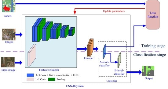
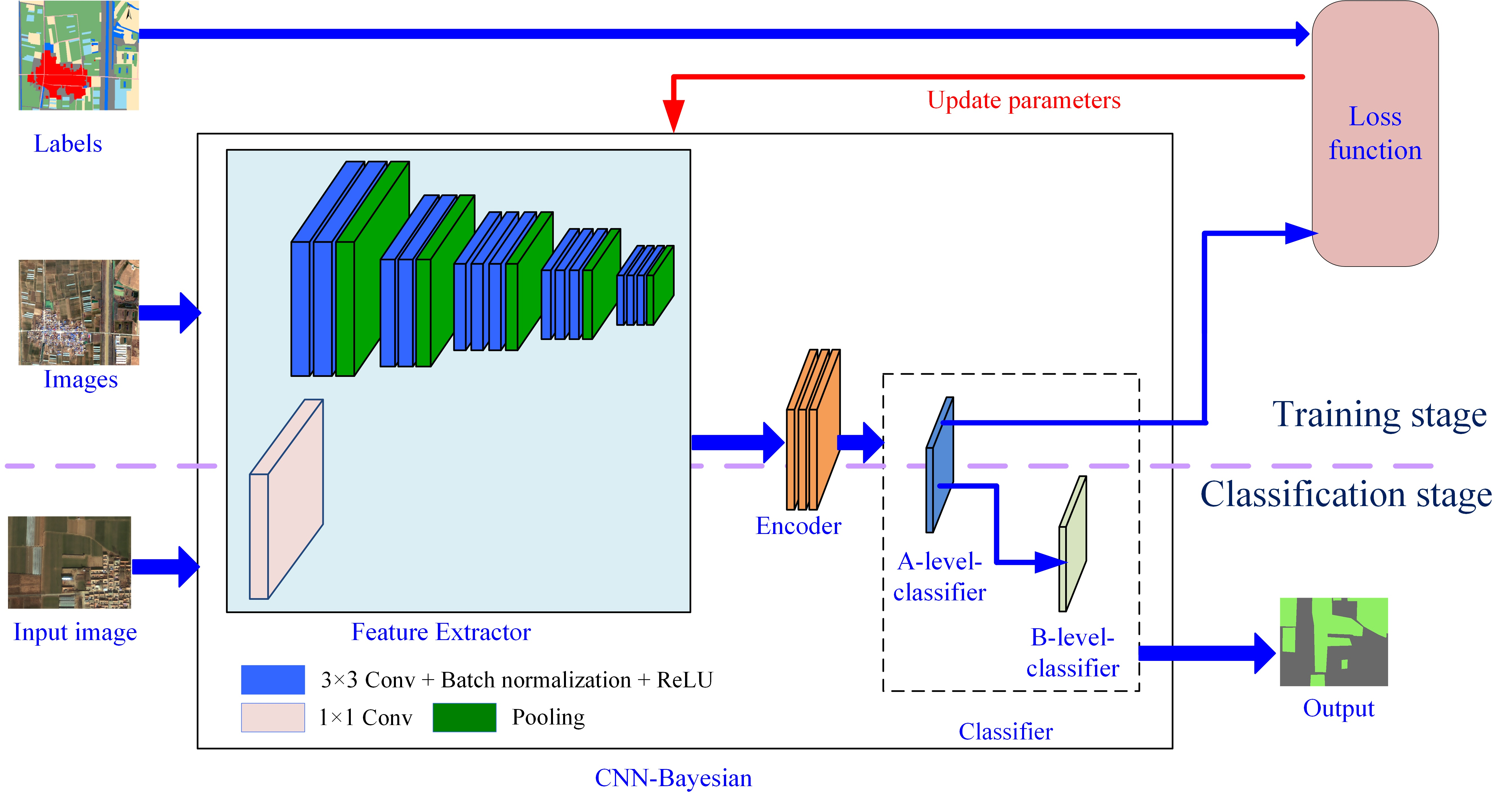
At present, the CNN structure used in the pre-pixel classification of remote sensing imagery generally includes two parts: feature extractor and classifier. The former has been the focus of many researchers with good results. The convolution value acquired by the convolution kernel and pixel block operations is regarded as a feature of central pixels in the pixel blocks and is the common technique for existing feature extractors. However, with regard to classifying pixels with acquired features, most studies have only used classifiers with relatively ordinary functions. These classifiers use a set of linear regression functions to encode the features of pixels and obtained category-code vectors. The SoftMax function is then used to convert the category-code vector into a category probability vector, and the category corresponding to the maximum probability value is taken as the pixel category.
Previous experimental results [44,45,46,47,48,49,50,51,52,53,54,55,56] have shown that misclassified pixels are primarily located at the intersections of two land use types, such as field edges or corners. This is because when the features of pixels in these areas are acquired, the used pixel blocks usually contain more pixels of other categories, resulting in the features often being different from the feature of inner pixels of the planting area, which frequently cause classification errors. By analyzing the probability vector of these misclassified pixels, it can be found that the difference between the maximum probability value and the second-maximum probability value is generally small. These errors are due to the inherent structure of the convolutional layer, which needs to be combined with the classifier to be improved.
The Bayesian model can synthesize information from different sources and improve the reliability of inferred conclusions [71,
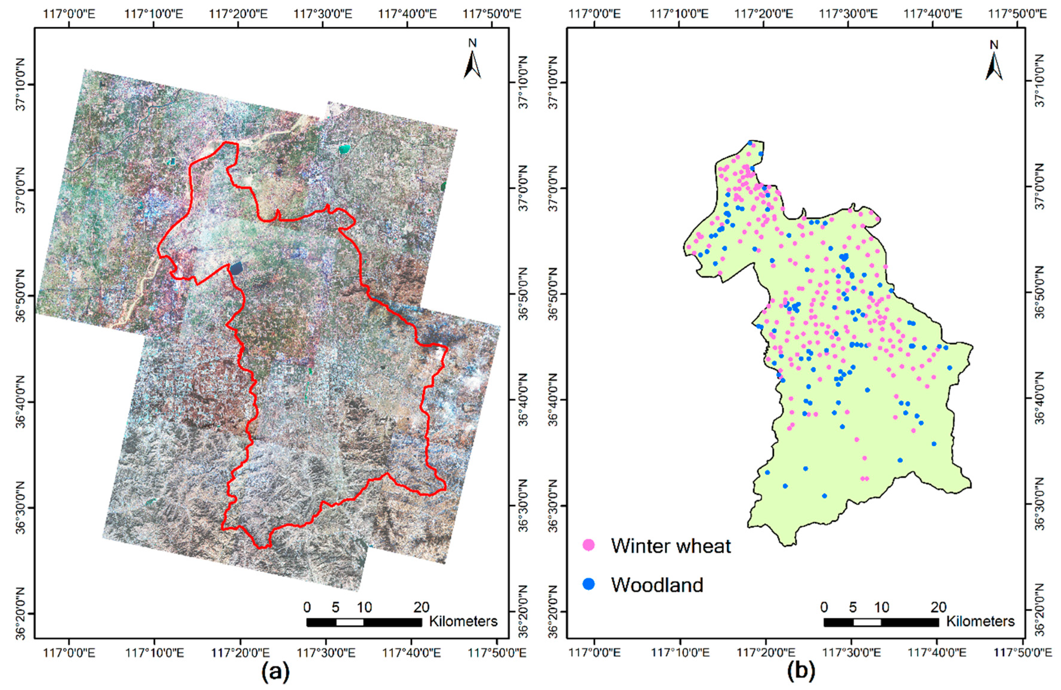
72]. Therefore, when judging the category of a pixel whose difference between the maximum probability value and the second-maximum probability value is small, the spatial structure information of the pixels can be further introduced to improve the reliability of the judgment by using the Bayesian model. In this study, we developed a new CNN consisting of a feature extractor, encoder, and a Bayesian classifier, which we refer to as a Bayesian Convolutional Neural Network (CNN-Bayesian model). We then used this model to extract winter wheat spatial distribution information from Gaofen 2 (GF-2) remote sensing imagery and compared the results with those achieved by other methods.

2. Study Area and Data

2.1. Study Area

Shandong Province is a major wheat-producing area in China. The total planted area was 38,303 km2 in 2016 and 38,429 km2 in 2017 (Figure 1) [73]. Zhangqiu County is located in North-central Shandong Province (36°25′–37°09′N, 117°10′–117°35′E). From south to north, the county’s terrain progresses through mountainous, hilly, plain, and lowland regions, accounting for 30.8%, 25.9%, 30.7%, and 12.6% of the total area, respectively. The main food crops are wheat and corn [74]. Moreover, the county’s geographical and agricultural conditions are representative of broader regions within China, making it an appropriate study area.

2.2. Data Sources

2.2.1. Remote Sensing Imagery

We used 32 GF-2 images to cover the entire Zhangqiu County; 17 were captured on 14 February, 2017, and 15 on 21 January and 1 March, 2018 (Figure 2a). Each GF-2 image is divided into a multispectral and panchromatic image. The former is composed of four spectral bands (blue, green, red, and near-infrared), and the spatial resolution of each multispectral image is 4 m, whereas that of the panchromatic image is 1 m.
The preprocessing of the GF-2 images involved four stages: geometric correction, radiometric calibration, atmospheric correction, and image fusion. Using Python and the Geospatial Data Abstraction Library, we designed a geometric correction program and completed this by combining the control points obtained from the ground investigation. Radiometric calibration converted the images’ digital values to absolute at-sensor radiance values using Environment for Visualizing Images (ENVI) software (developed by Harris Geospatial Solutions, Broomfield, Colorado, United States of America). The calibration parameters were obtained by calibration experiments in Chinese fields as published in CRESDA [9]. Atmospheric correction converted the radiance to reflectance using the Fast Line-of-Sight Atmospheric Analysis of Spectral Hypercubes (FLAASH) model in ENVI with the Interactive Data Language. The related FLAASH parameters were obtained according to the acquisition time and imaging conditions. Subsequently, the ENVI pan-sharpening method was used to fuse the multispectral and panchromatic images. After preprocessing, each fusion image had four bands (blue, green, red, and near-infrared) with a spatial resolution of 1 m and a size of 7300 × 6900 pixels.

2.2.2. Ground Investigation Data

The main land cover in Zhangqiu County during winter includes winter wheat, agricultural buildings, woodland, developed land, roads, water bodies, farmland, and bare fields. In fused GF-2 images, bare fields, agricultural buildings, developed land, water bodies, farmland, and roads are all visually distinct from each other and vegetated areas during winter. In order to accurately distinguish whether a vegetation area is winter wheat or woodland in visual interpretation, the sample information of winter wheat areas and woodland areas should be obtained, so we conducted ground investigations in 2017 and 2018, obtaining 367 sample points (251 winter wheat, 116 woodland); time, location, and land use were recorded for all points (Figure 2b).

2.3. Image-Label Datasets

We selected 305 non-overlapping region images from the GF-2 images described in Section 2.2 to establish the image-label dataset for training and test, and each image contained 1024 × 1024 pixels. The dataset covered all land use types of the study area, including winter wheat, agricultural buildings, woodland, developed land, roads, water bodies, farmland, and bare fields. We manufactured a label file for each image, which was used to record the category number of each pixel on the image. In combination with the ground investigation data described in Section 2.2.2, we used visual interpretation and ENVI software to establish the label file. Figure 3 illustrates a training image and corresponding label file.
In the label files, winter wheat, agricultural buildings, woodland, developed land, roads, water bodies, bare fields, and others were marked 1–8, respectively. In the test stage, 2–8 will be replaced by 9, indicating that the corresponding pixel is a non-winter wheat pixel.

3. Proposed CNN-Bayesian Model

3.1. Model Architecture

The proposed CNN-Bayesian model consists of a feature extractor used to generate feature vectors for each pixel, an encoder used to transform the feature vector of each pixel into a category-code vector, and a classifier used to determine the category of a pixel (Figure 4).

3.1.1. Feature Extractor

The feature extractor’s network structure is based on a VGG16 network [30] in that it consists of 13 layers (corresponding to the first 13 layers of a VGG16); each layer includes a convolution, batch normalization, activation, and pooling layer. Like a VGG16, the CNN-Bayesian model uses a rectified linear unit as an activation function. We added 10 convolution kernels (sized 1 × 1 × 3) in the first layer to extract the color features of pixels.
The input of the feature extractor is the fused GF-2 remote sensing images, each with four bands. The output is a 3D matrix with a size of m × n × l, where m and n are the number of rows and columns respectively, and l is the length of the feature vector of each pixel. Each feature vector corresponding to one pixel consists of three parts. The first is derived from the result of the convolution kernel, which represents the color feature. The second is derived from the result of the first layer, which represents the low-level texture features. The third is derived from the output of the last layer, which represents the semantic feature.
Compared with the camera image, the pixels of the remote sensing image are continuous. Therefore, we used the extension method to cut out the training and test images and then extend some pixels on the four edges of each image, to ensure that the size of the last layer’s feature image was the same as the original image.
We improved the original pooling method of VGG16 using the following equation:
a s , t = max i = s 1 , s , s + 1 j = t 1 , t , t + 1 b i , j ,
where s,t denotes the position of the pixel being calculated, a denotes the pooled result, and b denotes the feature map used in the pooled operation.
We used a step size of 1 in the pooling operation. After a feature map whose size is m × n has been pooled, the size of the resulting matrix is (m − 2) × (n − 2). Therefore, after each layer of feature extraction, the image size is reduced by four rows and four columns compared with the original image. Therefore, when we cut the training and test images, we extended 24 pixels outward on the four edges of each image.

3.1.2. Encoder

The encoder is used to transform the feature vector of a pixel from the feature extractor into a category-code vector, as shown below:
[ r 1 r 2 r m ] = [ w 11 w 12 w 1 n w 21 w m 1 w 22 w m 2 w 2 n w m n ] × [ x 1 x 2 x n ] T + [ b 1 b 2 b m ] ,
where each row of the matrix w indicates a fitting function for a specified class, m denotes the number of classes, n denotes the length of the feature vector of one pixel, vector x denotes the feature vector, vector b denotes the respective biases, and vector r denotes the encoded value. The matrix w and vector b are trained in the training stage.

3.1.3. Classifier

The classifier is divided into two levels, A and B. The A-level classifier transforms category-code vector r (corresponding to one pixel) into category-probability vector p as follows:
[ p 1 p 2 p m ] = [ e r 1 i m e r i e r 2 i m e r i e r m i m e r i ] ,
where m denotes the number of classes. Next, the confidence level (CL) of each p is calculated as follows:
C L = p i p j ,
where p i denotes the max value in p, and p j denotes the max value in p except p i . The category of a given pixel is determined by:
A o u t = { i ;     i n   t r a i n   s t a g e   a n d   p i   i s   t h e max v a l u e   i n   P   1 ;     i n   c l a s s i f i c a t i o n   s t a g e   a n d   C L δ 11 ;     i n   c l a s s i f i c a t i o n   s t a g e   a n d   C L < δ ,
where A o u t denotes the category number of one pixel, code 1 indicates winter wheat, code 11 indicates uncertainty, and δ indicates the low threshold value of CL. The δ value is selected and determined manually after the training has been completed, and the training results of all samples are statistically analyzed.
The B-level classifier is used to determine the category of a pixel whose CL <   δ , denoted by vPixel, by acquiring the maximum posterior probability of vPixel classified as winter wheat:
v w w = P ( c = w w | ) = P ( | c = w w ) P ( c = w w ) P ( ) ,
where v w w denotes the maximum posterior probability that the category of vPixel is winter wheat when the CL value is , c is the category, ww denotes winter wheat, denotes the CL value corresponding to the P of vPixel, p( |c=ww) represents the probability that the CL value is equal to in winter wheat pixels, p(c=ww) indicates the probability of winter wheat, and p( ) indicates the probability that the CL value is equal to in all pixels. Next, the maximum posterior probability of vPixel classified as non-winter wheat is acquired by:
v n w = P ( c = n w | ) = P ( | c = n w ) P ( c = n w ) P ( ) ,
where v n w denotes the maximum posterior probability that the category vPixel is not winter wheat when the CL value is , c, , and p( ) have the same meaning as in the Equation (6), nw denotes non-winter wheat, p( |c=nw) indicates the probability that the CL value is equal to in non-winter wheat pixels, and p(c=nw) indicates the probability of non-winter wheat.
In Equations (6) and (7), p( |c=ww), p(c=ww), p( |c=nw), p(c=nw), and p( ) are acquired by statistical methods. When obtaining p( |c=ww) and p( |c=nw), all samples are statistics, reflecting the global characteristics of the confidence of certain classes. When obtaining p(c=ww), p(c=nw), and p( ) , only samples in the maximum pixel block are used to extract the features of vPixel, reflecting the local characteristics of pixel spatial associations.
The classifier determines the final pixel category as follows:
o u t = { 1 ;   ( p 1   i s   t h e max v a l u e   i n   P     a n d   C L δ ) o r   ( C L < δ   a n d   v w w   > v n w )   o r   ( C L < δ   ,   v w w = v n w   a n d     p 1   i s   t h e max v a l u e   i n   P ) 9 ;           ( p 1   i s   n o t   t h e max v a l u e   i n   P     a n d   C L δ ) )     o r   ( C L < δ   a n d       v w w < v n w )   o r   ( C L < δ   ,   v w w = v n w   a n d     p 1   i s   n o t   t h e max v a l u e   i n   P ) ,
where o u t represents the final category number of one pixel, code 1 indicates winter wheat, and code 9 indicates non-winter wheat.

3.2. Training Model

The basic loss function calculation unit is the definition of cross entropy, expressed for one sample as:
H ( p , q ) = i = 1 8 q i l o g ( p i ) ,
where p is the predicted category probability distribution, q is the actual category probability distribution, and i is the index of an element in the category probability distribution. On this basis, the loss function of the CNN-Bayesian model is defined as:
l o s s = 1 t s t s i = 1 8 q i l o g ( p i ) ,
where ts denotes the pixel amount used in the training stage.
We trained the CNN-Bayesian model in an end-to-end manner, B-level classifier does not participate in the training stage. The parameters required for B-level classifier to perform calculations are obtained by statistics after training completed. The training stage consists of the following steps:
  • Image-label pairs are input into the CNN-Bayesian model as a training sample dataset, and parameters are initialized.
  • Forward propagation is performed on the sample images.
  • The loss is calculated and back-propagated to the CNN-Bayesian model.
  • The network parameters are updated using the stochastic gradient descent [45] with momentum.
Steps 2–4 are iterated until the loss is less than the predetermined threshold values.
Table 1 shows the hyperparameters setup we used to train our model. In the comparison experiments, the hyperparameters also applied to the comparison model.

3.3. Work Flow

First, a set of fixed-size pixel blocks are cut from the pre-processed remote sensing image set to form the image set for training and testing. The training images are labeled pixel by pixel using visual interpretation. These data are then used to train the CNN-Bayesian model (loss value of 10–9 in this study). The predicted category, actual category, and CL of each sample are output after each round of training. Subsequently, the training information of the last round is used to acquire the confidence threshold δ (0.23 in this study) and the probability distributions p( |c=ww) and p( |c=nw). Finally, the trained model is used to exact winter wheat spatial distribution information form remote sensing images.

4. Experimental Results

4.1. Experimental Setups

The proposed CNN-Bayesian model was implemented using Python 3.6 on a Linux Ubuntu 16.04 operating system and TensorFlow framework. The comparison experiments were performed on a graphics workstation with an NVIDIA GeForce Titan X Graphics device with 12 GB graphic memory.
The network architecture parameters of the feature extractor of CNN-Bayesian model and the data dimensions of each layer are given in Table 2.
SegNet [35] and DeepLab [37] are classic semantic segmentation models for images that have achieved good results in the processing of camera images. Moreover, the working principles of these two models are similar to that of our study, and we therefore chose these as comparison models to better reflect the advantages of our model in feature extraction and classification. We also removed the second-level classifier of the CNN-Bayesian model as another comparison model, named VGG-Ex, to better compare the role of the Bayesian classifier.
We used data augmentation techniques on the dataset to prevent overfitting, and each image was randomly processed in brightness, saturation, hue, and contrast. After the processing is completed, each image is rotated and transformed, and each image is rotated three times (90°, 180°, 270°). There are 6100 images in our final data set. We also employed random split technique for training and testing model to prevent overfitting. During each training and test round, 4880 images randomly selected from the image-label datasets were used as training data, and the remaining 1220 images were used as test data. The SegNet, DeepLab, VGG-Ex, and CNN-Bayesian model were trained with the same image dataset. This was done five times. Table 3 shows the total number of samples of each category used in each training and test round.

4.2. Results and Evaluation

Table 4 shows the confusion matrices for the segmentation results of the four models. Each row of the confusion matrix represents the proportion taken by the actual category, and each column represents the proportion taken by the predicted category. Our approach achieved better classification results. The proportion of “winter wheat” wrongly categorized as “non-winter wheat” was, on average, 0.033, and the proportion of “non-winter wheat” wrongly classified as “winter wheat” was, on average, 0.021.
In this paper, we used four popular criteria, named accuracy, precision, recall and Kappa coefficient to evaluate the performance of the proposed model [45]. Table 5 shows the values of evaluation criteria of the four models.
To further compare the classification accuracy of planting area edges, we further subdivided the categories into “inner” and “edge” labels. If only winter wheat category pixels are used in the convolution process to extract the pixel features, it is classified as inner; otherwise it is classified as edge. Table 6 show the confusion matrices for the segmentation results of the four models.
As can be seen from Table 4, the accuracy of inner category of four models’ results were similar, but the CNN-Bayesian model was more accurate with regard to the edge category. The accuracy of CNN-Bayesian model in edge recognition is three times higher than that of SegNet, two times higher than that of DeepLab. By comparing the accuracy of winter inner edge of CNN-Bayesian and that of VGG-Ex, it can be found that the ability of CNN-Bayesian to recognize winter wheat edge is improved by nearly 30% due to the use of Bayesian classifier.
Figure 5 shows ten images and corresponding results randomly selected from the tested images, each containing 1204 × 1024 pixels. The CNN-Bayesian model misclassified only a small number of pixels at the corner of the winter wheat planting area. In the DeepLab results and VGG-Ex results, the misclassified pixels were mainly distributed at the junction of winter wheat and non-winter wheat areas, including edge and corner locations, but the number of misclassified pixels in the VGG-Ex model results is less than that of the DeepLab. The SegNet results had the most errors, which were scattered throughout the image; most misclassified pixels were located on the edges and corners, with some also occurring in the planting area.

5. Discussions

This paper proposed a novel per-pixel classification approach to extract winter wheat spatial distribution from GF-2 imagery. This approach can extract winter wheat with fine field edge by using two strategies, including a CNN structure to extract features and a two-level classifier to determine the pixel’s category accurately. The contributions of these two strategies are discussed as follows.

5.1. The Effectiveness of Feature Extractor

To distinguish winter wheat from other categories, a popular deep learning algorithm CNN was applied to explore the features. The trained feature extractor of proposed CNN-Bayesian model has strong feature extraction ability, which can make the distances between feature vectors extracted from pixels of the same category, but with different spectral information, close, and make the distances between feature vectors extracted from pixels from different category, but with close spectral information, far away.
Since the CNN-Bayesian model and the VGG-Ex model use the same feature extractor, we selected the most different set of semantic features from the last layer of the CNN-Bayesian, SegNet, and DeepLab models for comparative analysis, Figure 6 show the statistical results, respectively. The degree of confusion in the CNN-Bayesian model results is smaller than that in the other two models because its network structure and data organization mode are better, and the improved pooling algorithm used in feature extractor has a larger receptive field, and has a greater advantage in feature aggregation than the classical pooling algorithm. The CNN-Bayesian model feature extractor can keep the size of the feature image of the last layer unchanged without using deconvolution. Furthermore, it can eliminate location errors of the feature value that may be caused by the deconvolution operation and ensure one-to-one correspondence between the feature value and the pixel, thus reducing the degree of confusion between the features of winter wheat edge and non-winter wheat areas. Compared with the comparison model, the CNN-Bayesian model better suits the data features of high-resolution remote sensing images.
As can been seen for the statistical result of SegNet, although the feature values of winter wheat inner pixels and winter wheat edge pixels are scattered, the feature values of winter wheat inner pixels are basically not overlapped with the feature values of other categories. However, the overlap between the feature values of winter wheat edge pixels and other categories is large, which is the reason that the accuracy of winter wheat inner higher than that of winter wheat edge.
The feature values of some winter wheat edge pixels were confused with those of non-winter wheat pixels in all three cases, but those of winter wheat inner pixels were never confused with those of non-winter wheat pixels. This shows that pixel position has a great impact on the feature extraction results, mainly for two main reasons: First, field edge pixel information is different from inner pixel information, because edge areas often contain both winter wheat and bare fields or other land use types, and the proportion of winter wheat varies greatly, whereas inner areas contain only winter wheat. Second, pixel blocks centered on pixels at the edge of winter wheat fields, usually contain more non-winter wheat than wheat pixels (Figure 7). Thus, when extracting the feature values of these edge pixels, approximately 50% of the pixels involved in the convolution operation are pixels of other categories, whereas the ratio for corners is 75% or higher.

5.2. The Effectiveness of Classifier

Both the CNN-Bayesian model and the comparison model use the category-probability vector as the basis for determining the category of the pixels. The main advantage of the CNN-Bayesian model is that it takes into account the deep meaning of the difference between elements of category-probability vector, and use hierarchical strategy to determine the category of the pixels. The category of pixels with high confidence were directly determined, and the category of pixels with low confidence were determined combining prior knowledge. VGG-Ex, SegNet and DeepLab only use the maximum probability value as the basis to determine the category of the pixels. Therefore, the strategy adopted by the CNN-Bayesian model helps to improve the accuracy of the results, and the results are shown and compared in Figure 5, Table 3 and Table 4.
We select the number of pixels in each confidence level of the CNN-Bayesian, VGG-Ex, SegNet, and DeepLab models for comparative analysis (Figure 8). The pixel ratio of the SegNet and DeepLab models is higher than that of the CNN-Bayesian model and VGG-Ex at a lower confidence level. This shows that the feature composition of the CNN-Bayesian model is more reasonable, because it uses color and texture features in addition to the high-level semantic features used by all three models.
As the confidence increases, the classification errors of the four models decrease and the degree of reduction increases (Figure 9). This is because the confidence value directly reflects the degree to which the pixel characteristics match the overall category characteristics and, thus, the likelihood that the classification result is correct. Therefore, it is reasonable to choose the confidence value as the index of the confidence that a given pixel will be classified into a certain category.
Overall, these results show that the CNN-Bayesian model is more capable than the comparison models, reflecting its advantageous use of a two-level classifier structure. Since the second-level classifier makes full use of the confidence and planting structure information, the number of misclassified pixels is effectively reduced.
As can be seen from Figure 8 and Figure 9, for the CNN-Bayesian model, the number of pixels with confidence lower than 0.23 is small, but the proportion of misclassification is very large. This is the reason we choose 0.23 as confidence threshold described in Section 3.3.

5.3. Comparison to Other Similar Works

At present, there are some methods focus on improving the classification accuracy of edge regions [43,44,45,67]. These methods describe the association between inputs from the semantic level, so that the relationship between prediction labels of adjacent pixels can be described, and the prediction results are not only related to the features of the predicted pixels. Also relevant, and affected by the results of previous predictions, our method can describe the statistical of inputs. The prediction result is determined by the features of the pixel itself and the regional statistical features, which is more in line with the characteristics of remote sensing data.

6. Conclusions

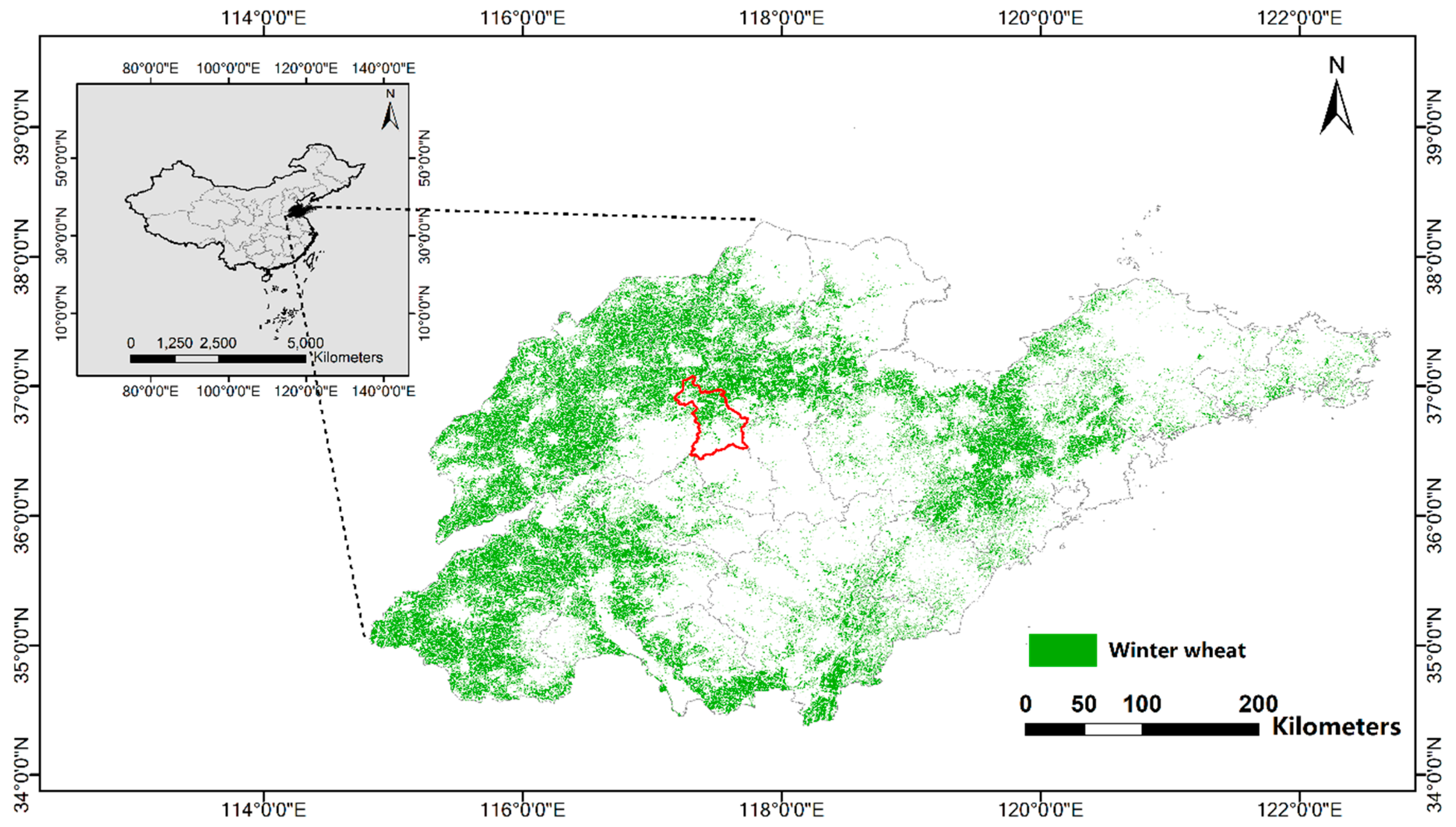
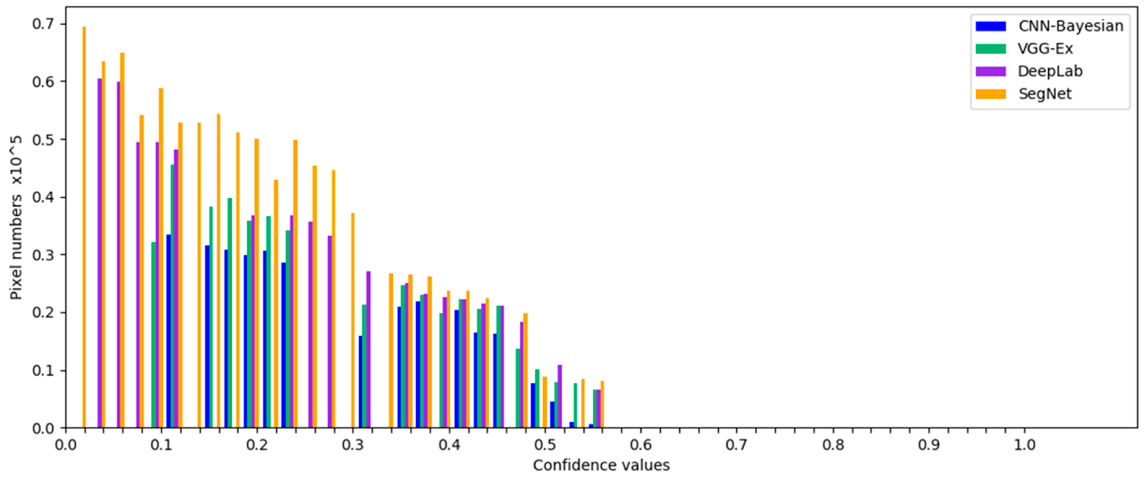
Using satellite remote sensing has become a mainstream approach for extracting winter wheat spatial distribution, but field edge results are usually rough, resulting in lowered overall accuracy. In this paper, we proposed a new approach for extracting spatial distribution information for winter wheat, which significantly improves the accuracy of edge extraction results. The main contributions of this paper are as follows: (1) Our feature extractor is designed to meet the characteristics of remote sensing image data, avoiding extra calculations and errors caused by using deconvolution in the feature extraction process. The feature extractor can fully explore the deep and spatial semantic features of the remote sensing image. (2) Our classifier effectively uses the confidence value of the category probability vector and combines the planting structure characteristics of winter wheat to reclassify pixels with a low confidence value, thus effectively reducing classification errors for edge pixels. As we optimized the method of extracting and using remote sensing image features and rationally used color, texture, semantic, and statistical features to obtain high-precision spatial distribution data of winter wheat. The spatial distribution data of winter wheat in Shandong Province in 2017 and 2018 obtained by the proposed approach has been used by the Meteorological Bureau of Shandong Province.
The number of categories that can be extracted by the proposed CNN-Bayesian model is determined by the number of categories of samples in the training dataset. When the model is used to extract other land use types or applied to another area, only a new training dataset is needed to retrain the model. The successfully trained model can then be used to extract high-precision spatial distribution data of land use from high-resolution remote sensing images.
The main disadvantage of our approach is that it requires more pre-pixel label files. Future research should test the use of semi-supervised classification to reduce the dependence on pre-pixel label files.

Author Contributions

Conceptualization: C.Z., F.L., and S.G.; methodology: C.Z.; software: C.Z. and F.L.; validation: S.G., Y.H., and D.S.; formal analysis: C.Z. and H.Z.; investigation: K.F.; resources: Y.H.; data curation: Y.Z.; writing—original draft preparation: C.Z.; writing—review and editing: F.L. and S.G.; visualization: K.F.; supervision: C.Z.; project administration: C.Z. and F.L.; funding acquisition: C.Z., F.L., and S.G.

Funding

This research was funded by the National Key R and D Program of China, grant number 2017YFA0603004; the Science Foundation of Shandong, grant numbers ZR2017MD018 and ZR2016DP04; the National Science Foundation of China, grant number 41471299; the Open Research Project of the Key Laboratory for Meteorological Disaster Monitoring, Early Warning and Risk Management of Characteristic Agriculture in Arid Regions, grant numbers CAMF-201701 and CAMF-201803; and the Key Project of Shandong Provincial Meteorological Bureau, grant number 2017sdqxz03.

Conflicts of Interest

The authors declare no conflict of interest.

References

  1. Websit of Food and Agriculture Organization of the United Nations. Available online: http://www.fao.org/faostat/zh/#data/QC (accessed on 8 August 2018).
  2. Announcement of the National Statistics Bureau on Grain Output in 2017. Available online: http://www.gov.cn/xinwen/2017-12/08/content_5245284.htm (accessed on 8 December 2017).
  3. Zhang, J.; Feng, L.; Yao, F. Improved maize cultivated area estimation over a large scale combining MODIS–EVI time series data and crop phenological information. ISPRS J. Photogramm. Remote Sens. 2014, 94, 102–113. [Google Scholar] [CrossRef]
  4. Chen, X.-Y.; Lin, Y.; Zhang, M.; Yu, L.; Li, H.-C.; Bai, Y.-Q. Assessment of the cropland classifications in four global land cover datasets: A case study of Shaanxi Province, China. J. Integnit. Agric. 2017, 16, 298–311. [Google Scholar] [CrossRef]
  5. Ma, L.; Gu, X.; Xu, X.; Huang, W.; Jia, J.J. Remote sensing measurement of corn planting area based on field-data. Trans. Chin. Soc. Agric. Eng. 2009, 25, 147–151. (In Chinese) [Google Scholar] [CrossRef]
  6. McCullough, I.M.; Loftin, C.S.; Sader, S.A. High-frequency remote monitoring of large lakes with MODIS 500 m imagery. Remote Sens. Environ. 2012, 124, 234–241. [Google Scholar] [CrossRef]
  7. Hao, H.E.; Zhu, X.F.; Pan, Y.Z.; Zhu, W.Q.; Zhang, J.S.; Jia, B. Study on scale issues in measurement of winter wheat plant area by remote sensing. J. Remote Sens. 2008, 12, 168–175. (In Chinese) [Google Scholar]
  8. Wang, L.; Jia, L.; Yao, B.; Ji, F.; Yang, F. Area change monitoring of winter wheat based on relationship analysis of GF-1 NDVI among different years. Trans. Chin. Soc. Agric. Eng. 2018, 34, 184–191. (In Chinese) [Google Scholar] [CrossRef]
  9. Wang, D.; Fang, S.; Yang, Z.; Wang, L.; Tang, W.; Li, Y.; Tong, C. A regional mapping method for oilseed rape based on HSV transformation and spectral features. ISPRS Int. J. Geo-Informat. 2018, 7, 224. [Google Scholar] [CrossRef]
  10. Georgi, C.; Spengler, D.; Itzerott, S.; Kleinschmit, B. Automatic delineation algorithm for site-specific management zones based on satellite remote sensingdata. Precis. Agric. 2018, 19, 684–707. [Google Scholar] [CrossRef]
  11. Wang, L.; Guo, Y.; He, J.; Wang, L.; Zhang, X.; Liu, T. Classification method by fusion of decision tree and SVM based on Sentinel-2A image. Trans. Chin. Soc. Agric. Mach. 2018, 49, 146–153. (In Chinese) [Google Scholar] [CrossRef]
  12. Qian, X.; Li, J.; Cheng, G.; Yao, X.; Zhao, S.; Chen, Y.; Jiang, L. Evaluation of the effect of feature extraction strategy on the performance of high-resolution remote sensing image scene classification. J. Remote Sens. 2018, 22, 758–776. (In Chinese) [Google Scholar] [CrossRef]
  13. Wang, L.; Xu, S.; Li, Q.; Xue, H.; Wu, J. Extraction of winter wheat planted area in Jiangsu province using decision tree and mixed-pixel methods. Trans. Chin. Soc. Agric. Eng. 2016, 32, 182–187. (In Chinese) [Google Scholar] [CrossRef]
  14. Guo, Y.S.; Liu, Q.S.; Liu, G.H.; Huang, C. Extraction of main crops in Yellow River Delta based on MODIS NDVI time series. J. Nat. Res. 2017, 32, 1808–1818. (In Chinese) [Google Scholar] [CrossRef]
  15. Xu, Q.; Yang, G.; Long, H.; Wang, C.; Li, X.; Huang, D. Crop information identification based on MODIS NDVI time-series data. Trans. Chin. Soc. Agric. Eng. 2014, 30, 134–144. (In Chinese) [Google Scholar] [CrossRef]
  16. Hao, W.; Mei, X.; Cai, X.; Du, J.; Liu, Q. Crop planting extraction based on multi-temporal remote sensing data in Northeast China. Trans. Chin. Soc. Agric. Eng. 2011, 27, 201–207. (In Chinese) [Google Scholar] [CrossRef]
  17. Feng, M.; Yang, W.; Zhang, D.; Cao, L.; Wang, H.; Wang, Q. Monitoring planting area and growth situation of irrigation-land and dry-land winter wheat based on TM and MODIS data. Trans. Chin. Soc. Agric. Eng. 2009, 25, 103–109. (In Chinese) [Google Scholar]
  18. Sha, Z.; Zhang, J.; Yun, B.; Yao, F. Extracting winter wheat area in Huanghuaihai Plain using MODIS-EVI data and phenology difference avoiding threshold. Trans. Chin. Soc. Agric. Eng. 2018, 34, 150–158. (In Chinese) [Google Scholar] [CrossRef]
  19. Yang, P.; Yang, G. Feature extraction using dual-tree complex wavelet transform and gray level co-occurrence matrix. Neurocomputing 2016, 197, 212–220. [Google Scholar] [CrossRef]
  20. Reis, S.; Tasdemir, K. Identification of hazelnut fields using spectral and Gabor textural features. ISPRS J. Photogramm. Remote Sens. 2011, 66, 652–661. [Google Scholar] [CrossRef]
  21. Naseera, M.T.; Asima, S. Detection of cretaceous incised-valley shale for resource play, Miano gas field, SW Pakistan: Spectral decomposition using continuous wavelet transform. J Asian. Earth. Sci. 2017, 147, 358–377. [Google Scholar] [CrossRef]
  22. Liu, Y.; Bian, L.; Meng, Y.; Wang, H.; Zhang, S.; Yang, Y.; Shao, X.; Wang, Bo. Discrepancy measures for selecting optimal combination of parameter values in object-based image analysis. ISPRS J. Photogramm. Remote Sens. 2012, 68, 144–156. [Google Scholar] [CrossRef]
  23. Blaschke, T.; Hay, G.J.; Kelly, M.; Lang, S.; Hofmann, P.; Addin, E.; Feitosa, R.; Meer, F.; Werff, H.; Coillie, F.; et al. Geographic Object-Based Image Analysis—Towards a new paradigm. ISPRS J. Photogramm. Remote Sens. 2013, 87, 180–191. [Google Scholar] [CrossRef]
  24. Wu, M.; Yang, L.; Yu, B.; Wang, Y.; Zhao, X.; Zheng, N.; Wang, C. Mapping crops acreages based on remote sensing and sampling investigation by multivariate probability proportional to size. Trans. Chin. Soc. Agric. Eng. 2014, 30, 146–152. (In Chinese) [Google Scholar] [CrossRef]
  25. You, W.; Zhi, Z.; Wang, F.; Wu, Q.; Guo, L. Area extraction of winter wheat at county scale based on modified multivariate texture and GF-1 satellite images. Trans. Chin. Soc. Agric. Eng. 2016, 32, 131–139. (In Chinese) [Google Scholar] [CrossRef]
  26. Liu, D.; Han, L.; Han, X. High spatial resolution remote sensing image classification based on deep learning. Acta Opt. Sin. 2016, 36, 0428001. (In Chinese) [Google Scholar] [CrossRef]
  27. Li, D.; Zhang, L.; Xia, G. Automatic analysis and mining of remote sensing big data. J. Surv. Mapp. 2014, 43, 1211–1216. (In Chinese) [Google Scholar] [CrossRef]
  28. Mas, J.F.; Flores, J.J. The application of artificial neural networks to the analysis of remotely sensed data. Int. J. Remote Sens. 2007, 29, 617–663. [Google Scholar] [CrossRef] [Green Version]
  29. Pacifici, F.; Chini, M.; Emery, W.J. A neural network approach using multi-scale textural metrics from very high-resolution panchromatic imagery for urban land-use classification. Remote Sens. Environ. 2009, 113, 1276–1292. [Google Scholar] [CrossRef]
  30. Liu, C.; Hong, L.; Chen, J.; Chu, S.; Deng, M. Fusion of pixel-based and multi-scale region-based features for the classification of high-resolution remote sensing image. J. Remote Sens. 2015, 5, 228–239. (In Chinese) [Google Scholar] [CrossRef]
  31. Huang, X.; Zhang, L. An SVM ensemble approach combining spectral, structural, and semantic features for the classification of high-resolution remotely sensed imagery. IEEE Trans. Geosci. Remote Sens. 2013, 51, 257–272. [Google Scholar] [CrossRef]
  32. Mountrakis, G.; Im, J.; Ogole, C. Support vector machines in remote sensing: A review. ISPRS J. Photogramm. Remote Sens. 2011, 66, 247–259. [Google Scholar] [CrossRef]
  33. Krizhevsky, A.; Sutskever, I.; Hinton, G.E. ImageNet classification with deep convolutional neural networks. Commun. ACM 2017, 60, 84–90. [Google Scholar] [CrossRef] [Green Version]
  34. Szegedy, C.; Liu, W.; Jia, Y.; Sermanet, P.; Reed, S.; Anguelov, D.; Erhan, D.; Vanhoucke, V.; Rabinovich, A. Going deeper with convolutions. In Proceedings of the 2015 IEEE Conference on Computer Vision and Pattern Recognition (CVPR), Boston, MA, USA, 7–12 June 2015. [Google Scholar] [CrossRef]
  35. Simonyan, K.; Zisserman, A. Very deep convolutional networks for large-scale image recognition. arXiv, 2014; arXiv:1409.1556. [Google Scholar]
  36. He, K.; Zhang, X.; Ren, S.; Sun, J. Deep residual learning for image recognition. In Proceedings of the IEEE Conference on Computer Vision and Pattern Recognition, Las Vegas, NV, USA, 26 June–1 July 2016; pp. 770–778. [Google Scholar] [CrossRef]
  37. Chang, L.; Deng, X.M.; Zhou, M.Q.; Wu, Z.K.; Yuan, Y.; Yang, S.; Wang, H. Convolutional neural networks in image understanding. Acta Autom. Sin. 2016, 42, 1300–1312. (In Chinese) [Google Scholar] [CrossRef]
  38. Fischer, W.; Moudgalya, S.S.; Cohn, J.D.; Nguyen, N.T.T.; Kenyon, G.T. Sparse coding of pathology slides compared to transfer learning with deep neural networks. BMC Bioinform. 2018, 19, 489. [Google Scholar] [CrossRef]
  39. Long, J.; Shelhamer, E.; Darrell, T. Fully convolutional networks for semantic segmentation. IEEE Trans. Pattern Anal. Mach. Intell. 2014, 39, 640–651. [Google Scholar]
  40. Badrinarayanan, V.; Kendall, A.; Cipolla, R. SegNet: A deep convolutional encoder-decoder architecture for image segmentation. arXiv, 2015; arXiv:1505.07293. [Google Scholar] [CrossRef]
  41. Ronneberger, O.; Fischer, P.; Brox, T. U-Net: Convolutional networks for biomedical image segmentation. arXiv, 2015; arXiv:1505.04597. [Google Scholar]
  42. Chen, L.; Papandreou, G.; Kokkinos, I.; Murphy, K.; Yuille, A.L. DeepLab: Semantic image segmentation with deep convolutional nets, Atrous convolution, and fully connected CRFs. IEEE Trans. Patt. Anal. Mach. Intell. 2018, 40, 834–848. [Google Scholar] [CrossRef]
  43. Visin, F.; Romero, A.; Cho, K.; Matteucci, M.; Courville, A. ReSeg: A recurrent neural network-based model for semantic segmentation. arXiv, 2016; arXiv:1511.07053. [Google Scholar]
  44. Zhang, L.; Wang, L.; Zhang, X.; Shen, P.; Bennamoun, M.; Zhu, G.; Shah, S.A.A.; Song, J. Semantic scene completion with dense CRF from a single depth image. Neurocomputing 2018, 318, 182–195. [Google Scholar] [CrossRef]
  45. Fu, G.; Liu, C.; Zhou, R.; Sun, T.; Zhang, Q. Classification for high resolution remote sensing imagery using a fully convolutional network. Remote Sens. 2017, 9, 498. [Google Scholar] [CrossRef]
  46. Fu, K.; Lu, W.; Diao, W.; Yan, M.; Sun, H.; Zhang, Y.; Sun, X. WSF-NET: Weakly supervised feature-fusion network for binary segmentation in remote sensing image. Remote Sens. 2018, 10, 1970. [Google Scholar] [CrossRef]
  47. Castelluccio, M.; Poggi, G.; Sansone, C.; Verdoliva, L. Land use classification in remote sensing images by convolutional neural networks. arXiv, 2015; arXiv:1508.00092. [Google Scholar]
  48. Nogueira, K.; Penatti, O.A.B.; Dos Santos, J.A. Towards better exploiting convolutional neural networks for remote sensing scene classification. Pattern Recognit. 2017, 61, 539–556. [Google Scholar] [CrossRef] [Green Version]
  49. Lin, H.; Shi, Z.; Zou, Z. Maritime semantic labeling of optical remote sensing images with multi-scale fully convolutional network. Remote Sens. 2017, 9, 480. [Google Scholar] [CrossRef]
  50. Sharma, A.; Liu, X.; Yang, X.; Shi, D. A patch-based convolutional neural network for remote sensing image classification. Neural Netw. 2017, 95, 19–28. [Google Scholar] [CrossRef]
  51. Gaetano, R.; Ienco, D.; Ose, K.; Cresson, R. A two-branch CNN architecture for land cover classification of PAN and MS imagery. Remote Sens. 2018, 10, 1746. [Google Scholar] [CrossRef]
  52. Duan, L.; Xiong, X.; Liu, Q.; Yang, W.; Huang, C. Field rice panicle segmentation based on deep full convolutional neural network. Trans. Chin. Soc. Agric. Eng. 2018, 34, 202–209. (In Chinese) [Google Scholar] [CrossRef]
  53. Jiang, T.; Liu, X.; Wu, L. Method for mapping rice fields in complex landscape areas based on pre-trained convolutional neural network from HJ-1 A/B data. ISPRS Int. J. Geo-Inf. 2018, 7, 418. [Google Scholar] [CrossRef]
  54. Hasan, M.M.; Chopin1, J.P.; Laga, H.; Miklavcic, S.J. Detection and analysis of wheat spikes using Convolutional Neural Networks. Plant Methods 2018, 14, 100. [Google Scholar] [CrossRef]
  55. Rzanny, M.; Seeland, M.; Wäldchen, J.; Mäder, P. Acquiring and preprocessing leaf images for automated plant identification: Understanding the tradeoff between effort and information gain. Plant Methods 2017, 13, 97. [Google Scholar] [CrossRef]
  56. Jiao, J.; Fan, Z.; Liang, Z. Remote sensing estimation of rape planting area based on improved AlexNet model. Comp. Meas. Cont. 2018, 26, 186–189. (In Chinese) [Google Scholar] [CrossRef]
  57. Huang, H.; Deng, J.; Lan, Y.; Yang, A.; Deng, X.; Zhang, L. A fully convolutional network for weed mapping of unmanned aerial vehicle (UAV) imagery. PLoS ONE 2018, 13, e0196302. [Google Scholar] [CrossRef]
  58. Huang, H.; Deng, J.; Lan, Y.; Yang, A.; Deng, X.; Wen, S.; Zhang, H.; Zhang, Y. Accurate weed mapping and prescription map generation based on fully convolutional networks using UAV imagery. Sensors 2018, 18, 3299. [Google Scholar] [CrossRef]
  59. Huang, H.; Lan, Y.; Deng, J.; Yang, A.; Deng, X.; Zhang, L.; Wen, S. A semantic labeling approach for accurate weed mapping of high resolution UAV imagery. Sensors 2018, 18, 2113. [Google Scholar] [CrossRef]
  60. Ha, J.G.; Moon, H.; Kwak, J.T.; Hassan, S.I.; Dang, M.; Lee, O.N.; Park, H.Y. Deep convolutional neural network for classifying Fusarium wilt of radish from unmanned aerial vehicles. J Appl. Remote Sens. 2017, 11, 042621. [Google Scholar] [CrossRef]
  61. Long, M.; Ou, Y.; Liu, H.; Fu, Q. Image recognition of Camellia oleifera diseases based on convolutional neural network & transfer learning. Trans. Chin. Soc. Agric. Eng. 2018, 34, 194–201. [Google Scholar] [CrossRef]
  62. Liu, T.; Feng, Q.; Yang, S. Detecting grape diseases based on convolutional neural network. J. Northeast. Agric. Univ. 2018, 49, 78–83. [Google Scholar] [CrossRef]
  63. Wang, Q.; Gao, J.Y.; Yuan, Y. Embedding Structured Contour and Location Prior in Siamesed Fully Convolutional Networks for Road Detection. IEEE Trans. Intell. Transp. 2018, 19, 230–241. [Google Scholar] [CrossRef]
  64. Ji, S.; Zhang, C.; Xu, A.; Shi, Y.; Duan, Y. 3D convolutional neural networks for crop classification with multi-temporal remote sensing images. Remote Sens. 2018, 10, 75. [Google Scholar] [CrossRef]
  65. Ndikumana, E.; Ho Tong Minh, D.; Baghdadi, N.; Courault, D.; Hossard, L. Deep recurrent neural network for agricultural classification using multitemporal SAR Sentinel-1 for Camargue, France. Remote Sens. 2018, 10, 1217. [Google Scholar] [CrossRef]
  66. Namin, S.T.; Esmaeilzadeh, M.; Najafi, M.; Brown, T.B.; Borevitz, J.O. Deep phenotyping: Deep learning for temporal phenotype/genotype classification. Plant Methods 2018, 14, 66. [Google Scholar] [CrossRef]
  67. Maggiori, E.; Charpiat, G.; Tarabalka, Y.; Alliez, P. Recurrent Neural Networks to Correct Satellite Image Classification Maps. arXiv, 2017; arXiv:1608.03440. [Google Scholar] [CrossRef]
  68. Peng, X.; Feng, J.S.; Xiao, S.J.; Yau, W.Y.; Zhou, J.T.; Yang, S.F. Structured AutoEncoders for Subspace Clustering. IEEE T Image Process 2018, 27, 5076–5086. [Google Scholar] [CrossRef] [PubMed]
  69. Wang, Q.; Meng, Z.T.; Li, X.L. Locality Adaptive Discriminant Analysis for Spectral-Spatial Classification of Hyperspectral Images. IEEE Geosci. Remote Sens. 2017, 14, 2077–2081. [Google Scholar] [CrossRef]
  70. Huang, Z.; Zhu, H.; Zhou, J.T.; Peng, X. Multiple Marginal Fisher Analysis. IEEE Trans. Ind. Electron. 2018. [Google Scholar] [CrossRef]
  71. Jung, M.C.; Park, J.; Kim, S. Spatial Relationships between Urban Structures and Air Pollution in Korea. Sustainability 2019, 11, 476. [Google Scholar] [CrossRef]
  72. Chen, M.; Sun, Z.; Davis, J.M.; Liu, Y.; Corr, C.A.; Gao, W. Improving the mean and uncertainty of ultraviolet multi-filter rotating shadowband radiometer in situ calibration factors: Utilizing Gaussian process regression with a new method to estimate dynamic input uncertainty. Atmos. Meas. Tech. 2019, 12, 935–953. [Google Scholar] [CrossRef]
  73. Website of Zhangqiu County People’s Government. Available online: http://www.jnzq.gov.cn/col/col22490/index.html (accessed on 21 October 2018).
  74. Calibration Parameters for Part of Chinese Satellite Images. Available online: http://www.cresda.com/CN/Downloads/dbcs/index.shtml (accessed on 29 May 2018).
Figure 1. Regional distribution of wheat planting in Shandong Province, China, and the location of Zhangqiu County (red outline).
Remotesensing 11 00619 g001
Figure 2. Data sources: (a) Gaofen 2 remote sensing imagery of Zhangqiu County; and (b) sample point locations within the county.
Remotesensing 11 00619 g002
Figure 3. Example of image classification: (a) original Gaofen 2 image and (b) classified by land use type.
Remotesensing 11 00619 g003
Figure 4. Architecture of the proposed CNN-Bayesian model; ReLU: rectified linear unit.
Remotesensing 11 00619 g004
Figure 5. Comparison of segmentation results for Gaofen 2 satellite imagery: (a) original images, (b) ground truth, (c) results of CNN-Bayesian, (d) results of VGG-Ex, (e) results of SegNet, and (f) results of DeepLab.
Remotesensing 11 00619 g005
Figure 6. Statistical results of the (a) CNN-Bayesian, (b) SegNet, and (c) DeepLab.
Remotesensing 11 00619 g006
Figure 7. Examples of the effect of pixel position on the extracted features; pixel boxes (red) centered on corner or edge areas contain 50% or more non-winter wheat pixels.
Remotesensing 11 00619 g007
Figure 8. Distribution of confidence values for the four models.
Remotesensing 11 00619 g008
Figure 9. Distribution of misclassified pixels for all four models.
Remotesensing 11 00619 g009
Table 1. The hyperparameters setup.
HyperparameterValue
mini-batch size32
learning rate0.0001
momentum0.9
epochs20,000
Table 2. Network architecture parameters of the feature extractor and data dimensions.
LayerOperationsParameters 1Data Dimension of InputData Dimension of Output
1Convolutionalf = 3 × 3 × 3, s = 1, d = 64748 × 748 × 3746 × 746 × 64
poolingf = 3 × 3, s = 1746 × 746 × 64744 × 744 × 64
2Convolutionalf = 3 × 3 × 64, s = 1, d = 64744 × 744 × 64742 × 742 × 64
poolingf = 3 × 3, s = 1742 × 742 × 64740 × 740 × 64
3Convolutionalf = 3 × 3 × 64, s = 1, d = 64740 × 740 × 64740 × 740 × 64
poolingf = 3 × 3, s = 1740 × 740 × 64738 × 738 × 64
4Convolutionalf = 3 × 3 × 64, s = 1, d = 128738 × 738 × 64736 × 736 × 128
poolingf = 3 × 3, s = 1736 × 736 × 128734 × 734 × 128
5Convolutionalf = 3 × 3 × 128, s = 1, d = 128734 × 734 × 128732 × 732 × 128
poolingf = 3 × 3, s = 1732 × 732 × 128730 × 730 × 128
6Convolutionalf = 3 × 3 × 128, s = 1, d = 128730 × 730 × 128728 × 728 × 128
poolingf = 3 × 3, s = 1728 × 728 × 128726 × 726 × 128
7Convolutionalf = 3 × 3 × 128, s = 1, d = 256726 × 726 × 128724 × 724 × 256
poolingf = 3 × 3, s = 1724 × 724 × 256722 × 722 × 256
8Convolutionalf = 3 × 3 × 256, s = 1, d = 256722 × 722 × 256720 × 720 × 256
poolingf = 3 × 3, s = 1720 × 720 × 256718 × 718 × 256
9Convolutionalf = 3 × 3 × 256, s = 1, d = 256718 × 718 × 256718 × 718 × 256
poolingf = 3 × 3, s = 1718 × 718 × 256716 × 716 × 256
10Convolutionalf = 3 × 3 × 256, s = 1, d = 512716 × 716 × 256714 × 714 × 512
poolingf = 3 × 3, s = 1714 × 714 × 512712 × 712 × 512
11Convolutionalf = 3 × 3 × 512, s = 1, d = 512712 × 712 × 512710 × 710 × 512
poolingf = 3 × 3, s = 1710 × 710 × 512708 × 708 × 512
12Convolutionalf = 3 × 3 × 512, s = 1, d = 512708 × 708 × 512706 × 706 × 512
poolingf = 3 × 3, s = 1706 × 706 × 512704 × 704 × 512
13Convolutionalf = 3 × 3 × 512, s = 1, d = 512704 × 704 × 512702 × 702 × 512
poolingf = 3 × 3, s = 1702 × 702 × 512700 × 700 × 512
Output 700 × 700 × 586
f denotes the size of the convolution/pooling kernel, s represents the step length, and d represents the number of convolution cores in this layer. Because the batch normalization and rectified linear unit layers do not change the size of the data dimensions, they are not listed in the table.
Table 3. Total number of samples of each category used in each training and test round.
CategoryNumber of Total Samples (Million)
Winter wheat1572
Agricultural buildings6
Woodland568
Developed land1199
Roads51
Water bodies57
Farmland1521
Bare fields1332
Table 4. Confusion matrix of the winter wheat classification.
ApproachPredictedWinter WheatNon-Winter Wheat
CNN-BayesianWinter wheat0.6690.021
Non-winter wheat0.0330.277
VGG-ExWinter wheat0.6310.059
Non-winter wheat0.0490.261
SegNetWinter wheat0.5740.116
Non-winter wheat0.0930.217
DeepLabWinter wheat0.6050.085
Non-winter wheat0.0630.247
Table 5. Comparison of the four models’ performance.
IndexCNN-BayesianVGG-ExSegNetDeepLab
Accuracy0.946 0.892 0.791 0.852
Precision0.932 0.878 0.766 0.837
Recall0.941 0.872 0.756 0.825
Kappa0.879 0.778 0.616 0.712
Table 6. Confusion matrix for winter wheat inner/edge classification.
ApproachPredictedWinter Wheat InnerWinter Wheat EdgeNon-Winter Wheat
CNN-BayesianWinter wheat inner0.542/0.001
Winter wheat edge/0.1270.02
Non-winter wheat0.0060.0270.277
VGG-ExWinter wheat inner0.539/0.012
Winter wheat edge/0.0920.047
Non-winter wheat0.0080.0410.261
SegNetWinter wheat inner0.532/0.035
Winter wheat edge/0.0420.081
Non-winter wheat0.0330.060.217
DeepLabWinter wheat inner0.538/0.026
Winter wheat edge/0.0670.059
Non-winter wheat0.0150.0480.247

