A Hierarchical Convolution Neural Network (CNN)-Based Ship Target Detection Method in Spaceborne SAR Imagery


1
School of Electronic and Information Engineering, Beihang University, Beijing 100191, China
2
School of Computer Science and Engineering, Beihang University, Beijing 100191, China
*
Author to whom correspondence should be addressed.
Remote Sens. 2019, 11(6), 620; https://0-doi-org.brum.beds.ac.uk/10.3390/rs11060620
Submission received: 29 January 2019
/
Revised: 9 March 2019
/
Accepted: 11 March 2019
/
Published: 14 March 2019
Abstract
:The ghost phenomenon in synthetic aperture radar (SAR) imaging is primarily caused by azimuth or range ambiguities, which cause difficulties in SAR target detection application. To mitigate this influence, we propose a ship target detection method in spaceborne SAR imagery, using a hierarchical convolutional neural network (H-CNN). Based on the nature of ghost replicas and typical target classes, a two-stage CNN model is built to detect ship targets against sea clutter and the ghost. First, regions of interest (ROIs) were extracted from a large imaged scene during the coarse-detection stage. Unwanted ghost replicas represented major residual interference sources in ROIs, therefore, the other CNN process was executed during the fine-detection stage. Finally, comparative experiments and analyses, using Sentinel-1 SAR data and various assessment criteria, were conducted to validate H-CNN. Our results showed that the proposed method can outperform the conventional constant false-alarm rate technique and CNN-based models.
1. Introduction
Synthetic aperture radar (SAR) is an active microwave sensor, whose resolution—both in range and azimuth—can be improved via the pulse compression technique and synthetic aperture principle, to obtain high resolution remote sensing images. Moreover, another advantage of SAR imaging is its ability to operate on an all-weather/all-day-and-night basis [1]. Its application has been of interest in a variety of fields [2,3], e.g., SAR-based ocean remote sensing is widely used for environmental monitoring, search and rescue, target recognition, etc. [4]. Spaceborne SAR can also be operated over long periods in wide-area and real-time observations. In this context, it became a fundamental system for ship target recognition [5,6,7,8].
Typical ship target recognition using SAR imagery involves land and sea segmentation, target detection, target recognition, etc. In a large SAR image, target detection can be based on the feature difference between targets and backgrounds. In this process, a minimum region in one target chip containing the whole target can be confirmed [9], and the other part is considered background. Obvious feature differences normally exist between target and background regions, i.e., grayscale, multi-resolution, polarization, phase, etc., which form the basis for the design of many target detection methods. Hu et al. analyzed multidimensional SAR information using a linear time-frequency (TF) decomposition approach [10]. Yuan et al. extracted the gradient ratio pattern for each pixel based on Weber’s law, and used the local gradient ratio pattern histogram (LGRPH) for SAR target recognition [11]. In addition, the conventional constant false alarm rate (CFAR) technique is a typical detection method based on the grayscale feature. However, complicated and cluttered backgrounds severely affect CFAR detection performance [12].
In recent years, ship target detection based on deep learning (DL) has been widely studied [13,14], using the typical model of convolutional neural network (CNN) [15]. Liu et al. [16] presented a ship detection method, namely sea-land segmentation-based convolutional neural network (SLS-CNN), which combines a SLS-CNN detector, saliency computation, and corner features. Furthermore, Zhao et al. [17] proposed a spaceborne SAR ship detection algorithm based on low complexity CNN. Some other well-known CNN-based target detection methods include faster region-CNN (Faster R-CNN), you only look once (YOLO) list model, etc. For example, Li et al. [18,19] improved detection performance using Faster R-CNN, to successfully provide a densely connected multi-scale neural network [19]. This method is used to solve multi-scale and multi-scene problems in SAR ship detection. Feature maps are fused by densely connecting different feature map layers, rather than information from single feature maps, which represent top-to-down feature map connections. The R-CNN method is used for target recognition in large scene SAR images [20]. Furthermore, Hamza and Cai used YOLOv2 for ship detection [21], which introduced a multitude of enhancements into the original YOLO model.
However, these methods may be no longer effective when ghost replicas exist in an imaged scene. The ghost phenomenon is an intrinsic effect of SAR’s ambiguity, both in azimuth and range [22,23]. Range ambiguity occurs when different backscattered echoes—one related to a transmitted pulse and the other due to a previous transmission—temporarily overlap during the receiving operation [24]. On the other hand, azimuth ambiguity is caused by the aliasing of each target’s Doppler phase history. The Doppler frequency, which is higher than pulse repetition frequency (PRF), may lead to azimuth ambiguity [25]. This phenomenon is particularly relevant for high reflectivity targets, which appears in SAR images as ghosts in low reflectivity areas [26]. Moreover, according to the ghost generating principle, it is similar to its real target, rendering discrimination difficult. Azimuth ambiguity is prominent due to the spaceborne SAR’s fast platform velocity and big azimuth Doppler bandwidth.
According to the ghost generating principle and characteristics, we provided a hierarchical CNN-based ship target detection method in spaceborne SAR imagery, i.e., H-CNN. Hierarchical processing includes two stages: the coarse detection and fine detection. First, regions of interest (ROIs) were extracted from a large imaged scene in the coarse-detection stage. Although most land and sea background-related clutter was removed, ghost replicas remained in the ROIs. Therefore, the fine detection stage was introduced to further refine target detection against ghost replicas. In the experiments, H-CNN was trained and tested using Sentinel-1 SAR data [27]. In the following sections we first discuss H-CNN parameter configuration for optimal detection results. Then, the feature extraction quality is analyzed. Detailed texture and abstract semantic information are extracted using different convolutional layer operations. Finally, we conduct detection experiments to validate the H-CNN, and compare it to conventional CFAR technique and CNN models.
2. Ghost Phenomenon in Spaceborne SAR
Spaceborne SAR is an applied formation of SAR in space. Spaceborne SAR has some characteristic differences compared to airborne SAR [28,29,30,31], e.g., the former image normally has large data size due to its large antenna beam irradiation range, etc.
Ghost is an image representation of SAR ambiguity in range or azimuth direction. When PRF is too high, successive pulses may be aliased in one pulse period [32]. The distance between the target and its range ambiguity ghost can be calculated as follows [33,34]:
where is the index of azimuth ambiguities, indicating the spatial location of ghost replicas in the azimuth direction, is the radar wavelength, is the PRF, is the Doppler rate, and is the Doppler centroid.
If the PRF is excessively low, the part of Doppler frequency higher than PRF is folded into the azimuth spectrum, resulting in the occurrence of azimuth ambiguity. Figure 1 illustrates azimuth ambiguity formation with azimuth antenna pattern and PRF. is the Doppler bandwidth and , where is the SAR platform velocity and is the antenna size in the azimuth direction. When is greater than the value of PRF, as shown in Figure 1, undersampling causes aliasing in the azimuth spectrum. Blue and red dashed curves denote the first left and right replicas due to the sampling, respectively.
The distance between azimuth ambiguity ghost and target can be calculated by Equation (2) [33,34]:
where is the slant range and is the SAR platform velocity.
Moreover, in the case of a scene where ships are moving on a smooth sea surface, bright targets against a dark background would be present in the SAR image. In such cases, ghosts are noticeably observed, and may impose severe difficulties during ship target detection.
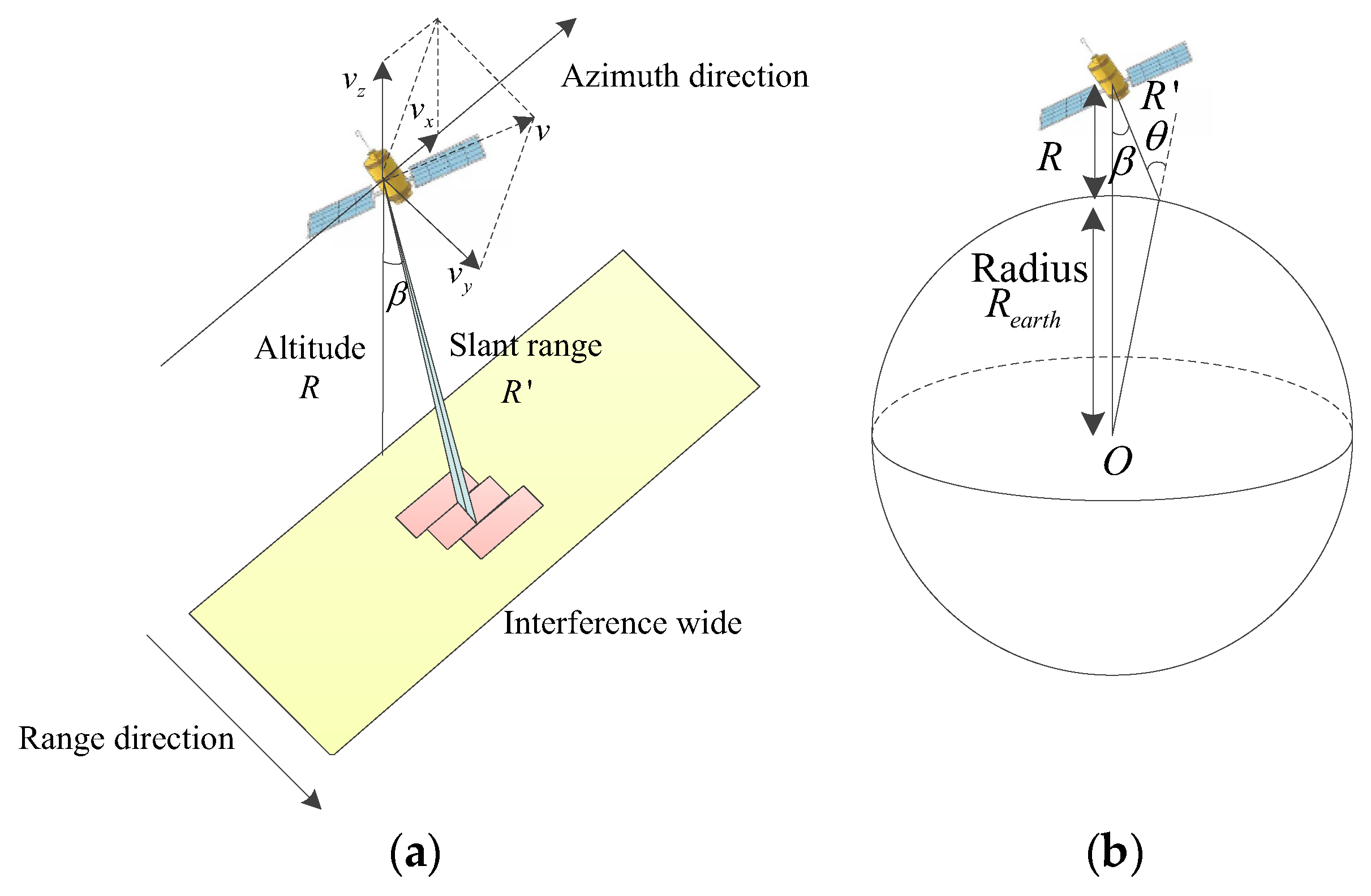
According to spaceborne SAR parameters, theoretical range and azimuth ambiguity distances can be estimated by Equations (1) and (2), respectively. Taking for instance Sentinel-1 SAR data, we analyze its azimuth ambiguity in some SAR images. Its imaging geometry is shown in Figure 2a. Although it contains four imaging modes, we only show the interferometric wide (IW) swath mode. Moreover, Sentinel-1 SAR system parameters play a significant role in the imaging, which contain platform speed, altitude of satellite to earth ground , elevation angle , PRF, etc. Table 1a,b show the Sentinel-1 satellite SAR system and a ship’s example parameters, respectively. Three different PRFs exist in one group of Sentinel-1 data. Furthermore, according to the characteristics of spaceborne SAR, slant range is influenced by the Earth’s curvature and distance from ground to satellite—their relationship is shown in Figure 2b. In other words, it can therefore be calculated using the satellite’s altitude from the Earth’s ground, radius of the Earth , elevation angle, and incidence angle .
Theoretical azimuth ambiguity distance can be obtained using Equation (2). When , the results in the cases of three PRF are ~5031.4 m, 4254.9 m, and 4940.6 m, respectively. The right graph of Figure 3 depicts the SAR image of the ship example and corresponding ghost replicas. We then extracted the azimuth direction sequence in one fixed range direction cell. In order to decrease the dynamic range of amplitude in azimuth direction, we expressed it in decibels. Finally, the sequence in azimuth direction is shown in the left graph of Figure 3. The distances between two ghosts and their target are approximately estimated to be ~4630 m and 4970 m, respectively, which are close to theoretical values mentioned above.
Discrimination difficulty is due to the fact that some traditional characteristics of a target and its corresponding ghost are similar, i.e., length–width ratio, area and shape complexity, etc. [35,36,37]. We therefore need to dispose of special discrimination between target and ghost, to eliminate the negative effects of ghosts on the detection performance.
3. Property Analyses of Ship Target and Ghost Replica
Some traditional characteristics are similar between a target and its corresponding ghost, i.e., length–width ratio, area and shape complexity, etc. It is therefore necessary to analyze their differences. The proposed method in this paper was designed based on the amplitude information in space dimension. Thus, we discuss the amplitude statistical feature of target chips and their ghost replicas. Amplitude distribution differences between target and ghost highlight their degree of distinction. In other words, a more obvious amplitude distribution difference makes the discrimination between target and ghost easier. First, one-to-one target chips and ghost replicas were collected from Sentinel-1 SAR data, all of which contain 100 groups. Amplitude normalization was performed for comparison convenience. For ghost replicas and target chips, the ratio of point number in the corresponding amplitude range to the overall pixel number was calculated as shown in Figure 4. Moreover, we enlarged local distribution results in the range of normalized amplitude from 0 to 0.02, which demonstrated that the amplitudes of most pixels are in this region. We found that the two distribution formations are similar, in that they first increase and then decline. When the normalized amplitude is higher than 0.02, the proportion difference of two distributions decreases and all the values are close to zero.
4. Architecture of the H-CNN Model
Traditional CNN consists of convolutional, pooling, and fully connected layers. The convolutional layer is used for feature extraction. Many convolutional kernels exist in every convolutional layer, and each pixel of kernel corresponds to one weight and one bias. Each neuron in the convolutional layer must be connected to several neighboring regions of the front layer. In addition, kernel size decides region size. In convolutional operation, kernels regularly slide in the whole feature map and feature extraction is realized as:
where and are the input and output results in pixel of the lth convolutional layer, respectively. They are all named as feature maps. In addition, and are weight and bias of convolutional kernel in convolutional layer l, respectively. is an activation function which is usually designed as sigmoid, rectified linear unit (ReLU) [38], etc. In this paper, ReLU is selected and is defined by:
After convolutional layer feature extraction, feature maps are transmitted to the next pooling layer. The pooling operation is used for selecting a few points to replace the whole feature map. Classic pooling methods include max pooling—which we applied in this paper—mean pooling, etc.
Finally, feature maps are fully connected in the last layer, which is similar to the hidden layer of traditional feedforward neural network. In this layer, multi-dimensional feature map structures are reshaped.
Traditional CNN is a supervised network. It is usually optimized by the well-known stochastic gradient descent (SGD) algorithm [39,40], which is basically an improved version of the batch gradient descent (BGD) method. In every iterative procedure, all samples were computed using this optimization algorithm. Moreover, to solve the slow update problem, a group of samples were stochastically selected and used for gradient direction determination in one iterative procedure. In the next iteration, a new group of stochastically selected samples was applied for the parameter update. When the loss of function arrives at the minimum value and remains stable, all parameters, i.e., weight and bias, are confirmed.
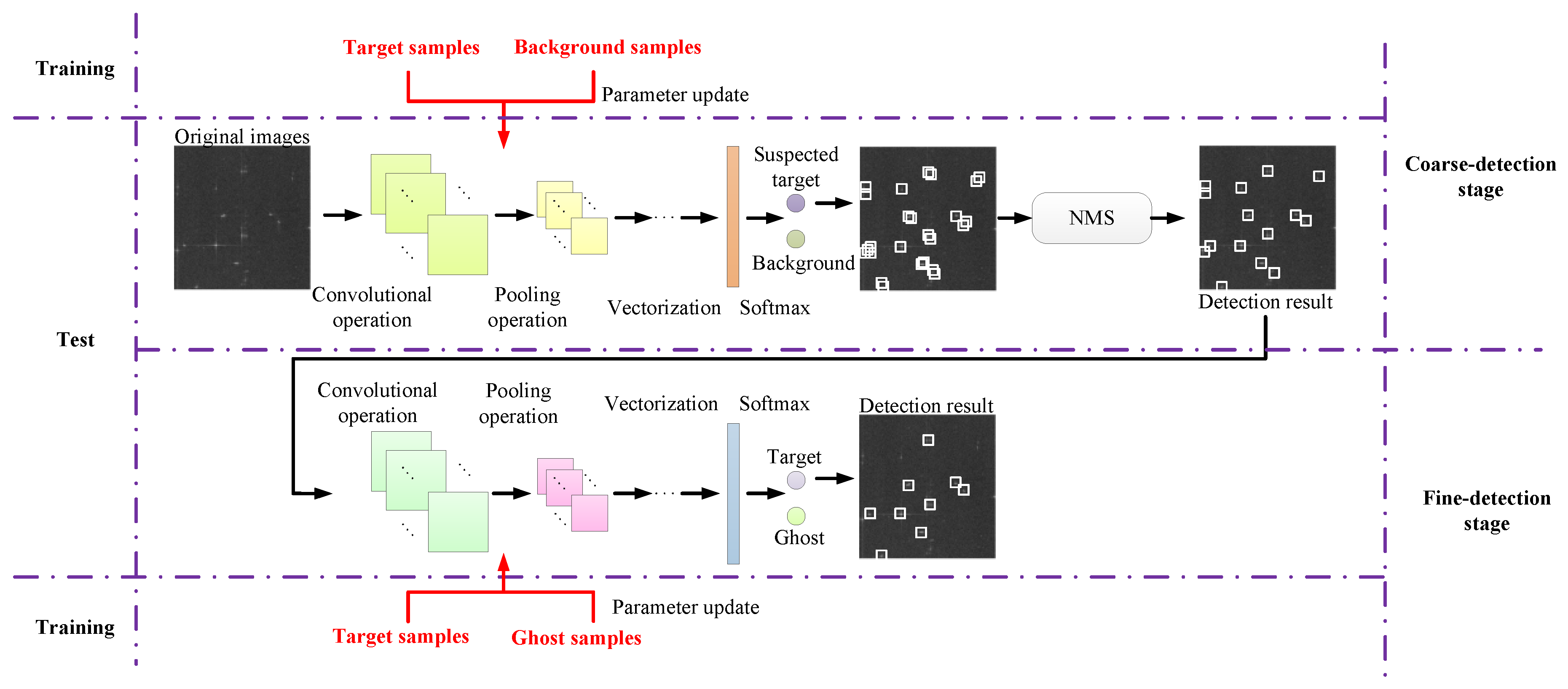
In this paper, we provide the H-CNN method for ship target detection in the spaceborne SAR imagery, with the hierarchical training pattern. The first coarse-detection stage of H-CNN was used to discriminate between ROIs and background. The ship targets were further determined from the interference of ghost replicas during the fine-detection stage. In the test phase, the whole SAR image was cut into several chips, and processed using coarse- and fine-detection stages, during which ship targets are extracted from the whole SAR. Here, all SAR chips were input in the coarse-detection stage. The chips were extracted when different from background. In order to further mitigate ghost interference, chips extracted after the coarse-detection stage were discriminated during the fine-detection stage for the ship target detection. It should be noted that large quantities of sea chips were always present. Therefore, the coarse detection could ease the computational burden for the following step by removing plenty of background chips. Furthermore, the fine-detection stage focuses on the elimination of ghost interference. However, since the sliding step is smaller than chip size, the overlapping phenomenon may occur. We used non-maximum suppression (NMS) [41] to further dispose of coarse-detection stage results. Architecture of the H-CNN model is shown in Figure 5.
During the coarse-detection stage, the network was trained using target and background samples. This part of the network mainly focuses on ROI extraction from a large imaged scene. Since unwanted ghost replicas are major interference sources that remain in ROIs, coarse-detection stage outputs are inputs into the fine-detection stage network, which facilitates the discrimination between real targets and ghosts. In the meantime, the fine-detection stage network is trained using target and ghost samples. NMS is disposed to all ROIs, which are extracted during the coarse-detection stage. Based on this process, ship target detection in spaceborne SAR imagery can be realized.
5. Experiments and Results
5.1. Dataset
In order to verify the effectiveness of proposed method, we applied it to Sentinel-1 SAR data [27]. Sentinel-1 satellite is an Earth observation satellite from the European Space Agency Copernicus Project. It consists of two satellites: Sentinel-1A and Sentinel-1B, and carries C-band SAR, which can provide continuous images in all-weather/all-day-and-night conditions. Nowadays, a series of operational services can be provided by Sentinel-1 SAR data, which include mapping of arctic sea ice and daily sea ice, marine environment monitoring, ground motion risk monitoring, forest mapping, etc. In this study, we collected data in the IW model, as shown in Figure 2. Its resolution was 5 m × 20 m, imaging field width is 250 km, and orbit altitude is 693 km.
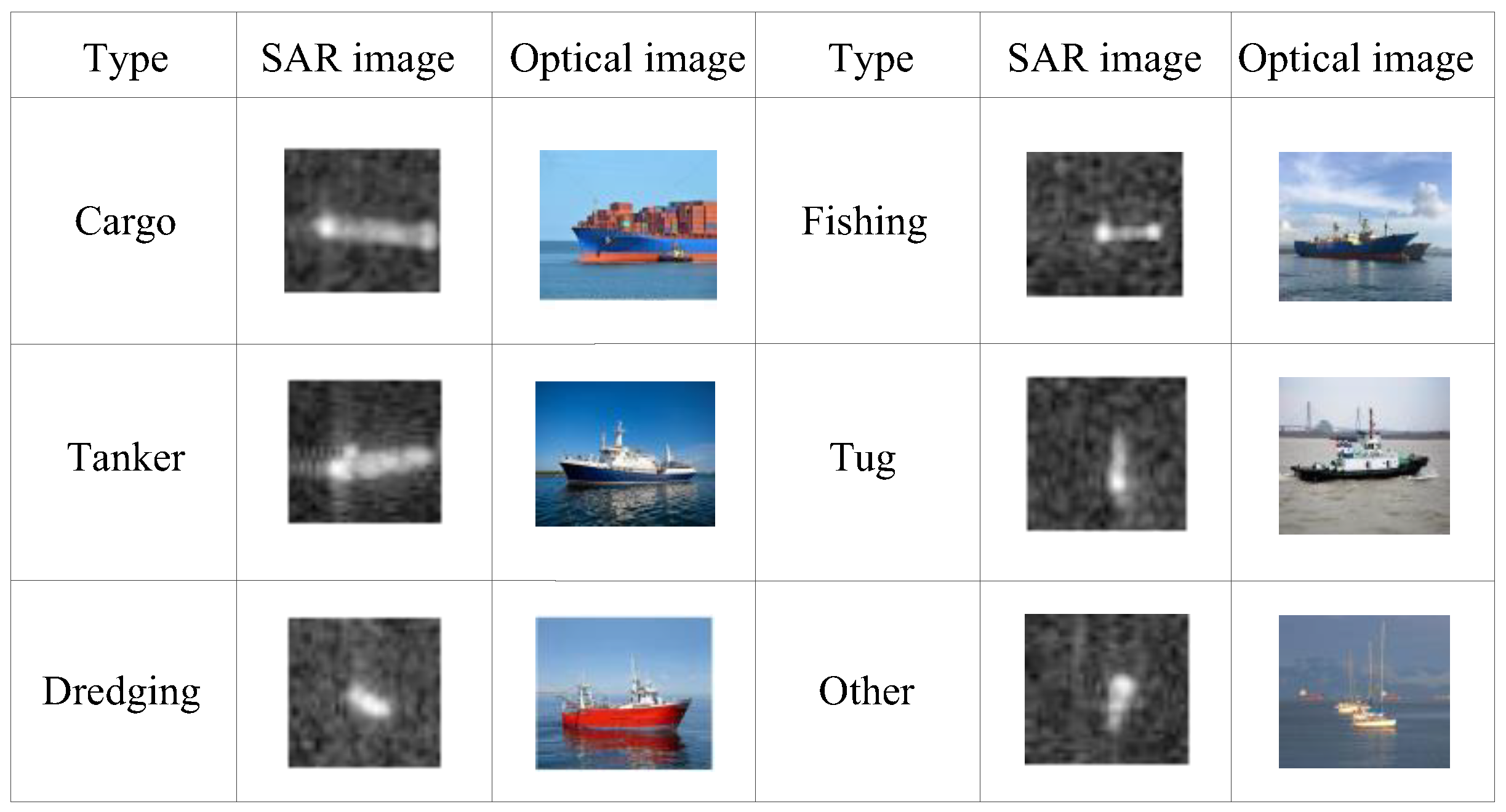
To further ensure the training samples’ reliability, each ship in the target sample set was verified using the Australian Maritime Safety Authority’s (AMSA) information [42]. These ship samples are collected in three Australian regions (North West, Great Australian Bight, and Bass Strait), which are indicated by white rectangles in Figure 6. To further guarantee the high diversity of ship types, we elaborate ship types using information provided on the AMSA website. For example, six-type ship SAR data are confirmed, i.e., cargo, tanker, dredging ship, fishing ship, tug, and other.
Some samples of SAR target images and their corresponding optical images are shown in Figure 7. In most cases, cargo and tanker are larger than other ships, and thus their structures in SAR images are obvious. On the other hand, the dredging ship is small, which is indicated by the SAR and optical images.
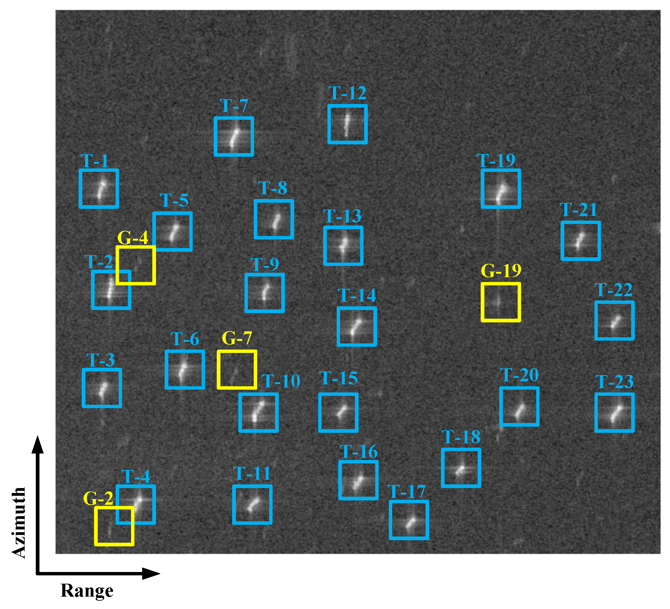
Ghost samples are extracted based on the corresponding target positions. Figure 8 shows a SAR image used in the test, where target chips and ghost replicas are highlighted by blue and yellow squares, respectively. In order to present the corresponding relationship, we labeled target as T-i, where the target chip is i. The ghost is labeled as G-i, where the ghost replica is i. We can identify 23 ship targets and 4 ghost replicas in this image. On this basis, target chips, ghost replicas, and background chips were collected, which contained 350 samples with the size of 40 pixels × 40 pixels, respectively, and were used for H-CNN training. Additional 149 Sentinel-1 SAR images with the size of 670 pixels × 643 pixels were applied to test the proposed networks performance. Altogether, 480 ships chips and 304 ghost replicas were present. To verify the effectiveness of H-CNN, training samples and test SAR images were acquired from different Sentinel-1 SAR data. The ship targets were confirmed by the maritime information on the AMSA website. Furthermore, we gained approximate corresponding ghost information based on the spaceborne SAR imaging theory, Sentinel-1 system parameters, and maritime information. The ghost confirmation method is shown in Section 2.
5.2. Discussion of Parameter Configuration of H-CNN
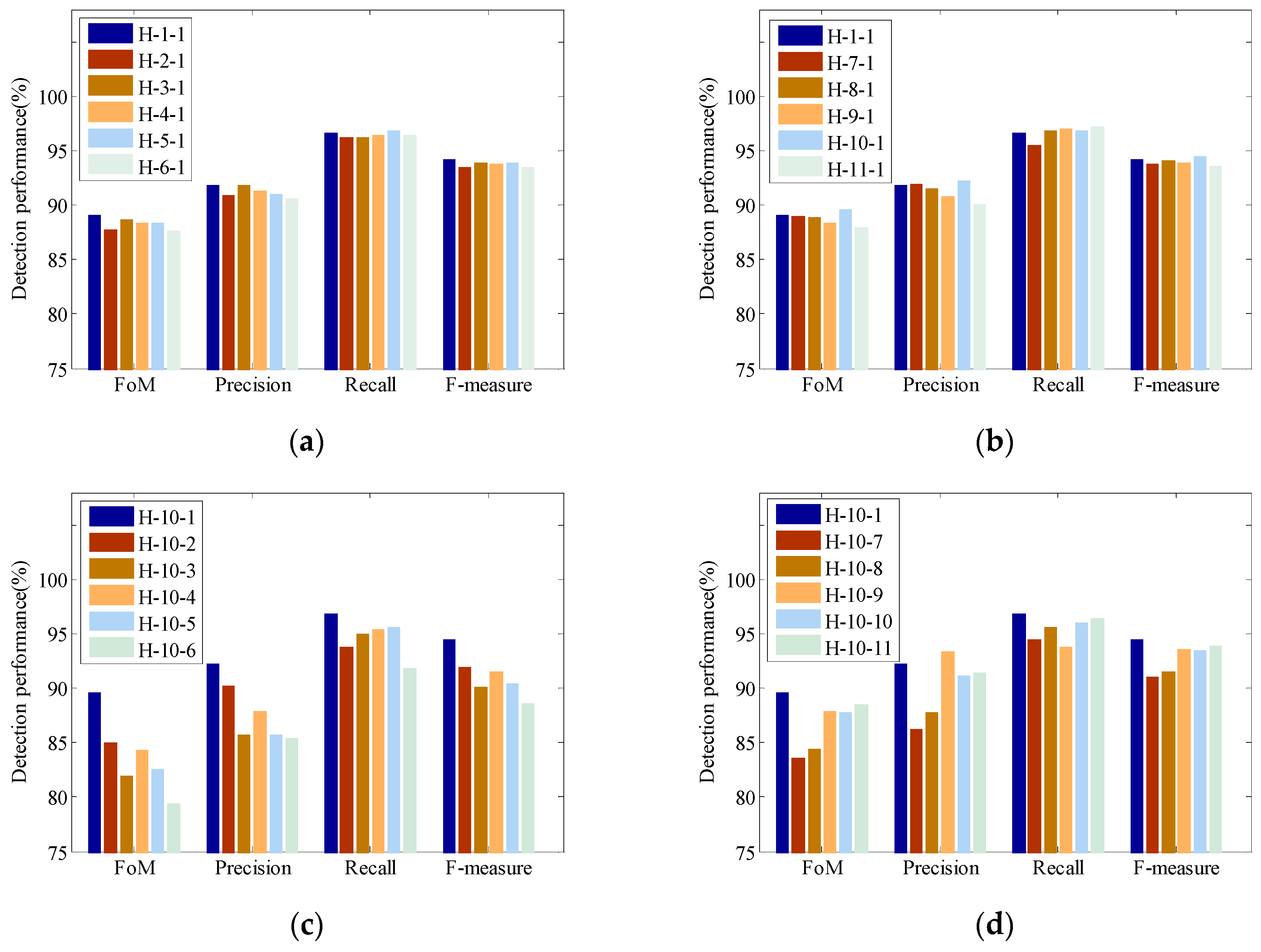
The key point of the proposed method is to mitigate the influence of ghost replicas on CNN models’ detection performance. Particularly, hyperparameters of convolutional kernels play a key role in the H-CNN performance. In this part, we studied H-CNN configurations with a variety of kernel hyperparameters to obtain its optimal detection performance. Details of kernel hyperparameters involved in H-CNN are shown in Table 2. In order to conveniently present different parameter configurations, we defined a brief description of network structure as H-i-j. It presents structure cases i and j in coarse- and fine-stage detection, respectively. We discuss the influence of kernel numbers and sizes during coarse- and fine-detection stages on detection performance, respectively. Moreover, in each layer, the structure is shown as A@B × B-Maxpool C × C formation, where kernel number is A, the kernel size is B × B, and max-pool is operated in each region of C × C. Different networks were trained by the same samples. We only changed kernel numbers of the coarse-detection stage and other parameters were fixed, as shown in Table 2a. According to the detection results, we confirmed the optimal kernel numbers and sizes during the coarse-detection stage using network comparisons shown in Table 2b. Similarly, kernel numbers and sizes during the fine-detection stage were confirmed using network comparisons shown in Table 2c,d. Detection performance was evaluated using four typical measures, including figure of merit (FoM), precision, recall, and F-measure [19,43], respectively. They are defined as follows:
where is the number of correct detected targets, denotes the number of falsely detected targets, and is the number of undetected targets.
Figure 9a illustrates detection results of H-1-1, H-2-1, H-3-1, H-4-1, H-5-1, and H-6-1. According to Table 2a, we identified differences in kernel numbers in stage1, while other parameters were similar. Hence, we could confirm kernel numbers during the coarse-detection stage by applying this comparison. Results in terms of FoM, precision, and F-measure showed that the optimal situation is H-1-1. As to the assessment in recall, H-1-1 is the second best one, but very close to H-5-1, which has the highest value in Figure 9a. It illustrates that compared to 4, 6, 8, 9, and 12, 3 is the best kernel number choice during coarse-detection stage. Therefore, the kernel number during coarse-detection stage was set to be 3 for the following comparison experiments.
According to Table 2b, kernel sizes alone during the coarse-detection stage in H-1-1, H-7-1, H-8-1, H-9-1, H-10-1, and H-11-1 were different. Hence, we could confirm this parameter via the detection results, which are shown in Figure 9b. Detection results of H-10-1 have a little superiority, i.e., best kernel size results are 11 × 11 and 8 × 8 in two layers of the coarse-detection stage.
On this basis, we further compared the results using different kernel numbers during the fine-detection stage, as shown in Table 2c. H-10-1 results are the best, indicating 3 as the kernel number during the fine-detection stage.
Finally, we discuss the influence of kernel size during the fine-detection stage on detection performance. According to Figure 9d, H-10-1 shows the best result, thus representing that the two layers kernel size during the fine-detection stage should be designed as 9 × 9.
5.3. Analyses of Feature Extraction by H-CNN
To analyze feature extraction quality, we first observed feature maps of target, background, and ghost chips. Figure 10 shows some feature map examples of H-CNN during the test. The target and ghost chips had clear boundaries compared to the background chip, thus the first layer’s feature maps both in coarse- and fine-detection stages had obvious texture in target and ghost chips. On the other hand, feature maps in the last layer presented abstract semantic information. We found that feature maps of target and ghost in the last layer were hardly discriminated during the coarse-detection stage. However, feature map differences between target and background were obvious, thus target and background discrimination was easy to detect during the coarse-detection stage. During the fine-detection stage, feature maps differences between target and ghost in the last layer became more obvious, thus their discrimination difficulty decreased.
In this part, we investigated the feature extraction quality of target chips and ghost replicas. If features are significantly different, the degree of distinction between two chips improves. The chips introduced in Section 3 were disposed by H-CNN and we collected their feature maps. The amplitude distribution was obtained by the same method. Distributions are shown in Figure 11. Amplitude for most focus points on the two regions, 0–0.02 and 0.96–1, are enlarged. The two distributions are dissimilar, especially in these two enlarged parts. Compared to Figure 4, distribution differences are obvious in Figure 11. It indicates that the distinguishable degree of features extracted by H-CNN is stronger than that of the original chips.
In order to further quantitatively analyze feature extraction quality, we introduced a linear discrimination analyses (LDA) theory. It is well known that LDA is aimed at maximizing between-class to within-class scatter matrices ratio. Here, two scatter matrices, called the within-class and between-class scatter matrices, are defined as [44]:
where is the within-class scatter matrices, is the between-class scatter matrices, is the samples i, is the mean value, is the type number, is the sample number ratio to all sample numbers, is the mean value matrix of samples, and is the mean value matrix of all samples.
Furthermore, there are two criteria for evaluating feature extraction quality, and , as follows:
where is the operation of calculate matrix trace. According to the LDA theory, the bigger and , the stronger distinguishable degree it has. Taking fine-stage detection for instance, we calculated and of a feature map in two layers as shown in Table 3. It is obvious that criteria values of the L2 layer were bigger than those of L1 layer. In other words, features in the L2 layer had a stronger distinguishable degree than those in the L1 layer.
5.4. Detection Result Comparison
Comparative analyses of CFAR, traditional CNN, low complex CNN, and the proposed network are presented herein to validate the H-CNN. In the CFAR method, we used the cell average CFAR (CA-CFAR) to detect above SAR images [45] where the false alarm rate was set as 1 10−3. Moreover, the traditional CNN model consisted of two convolutional layers, two pooling layers, and one fully connected layer. Its parameter configuration was confirmed by detection result comparisons of multiple networks. Moreover, a low complex CNN was introduced by [17]. H-CNN parameter configuration was set as aforementioned H-10-1.
In order to intuitively observe detection results based on different methods, we provided one instance as shown in Figure 12. It illustrates detection results of the SAR image of Figure 8, where targets and ghosts are labeled. We can see that all targets were detected, but the performance on ghosts was different. Hence, let us focus on the detection results of ghost replicas. G-2 was accurately detected as a ghost replica by these four methods. Other ghosts may be falsely detected by CFAR, traditional CNN, or low complexity CNN. For example, G-4 was identified as a target by CFAR, G-7 was also identified as a target by CFAR and traditional CNN. Only H-CNN was able to discriminate G-19 as a ghost replica. In other words, H-CNN could resist the interference of ghost replica and its detection performance outperforms other detection methods.
Furthermore, we calculated the statistical results to accurately illustrate detection performance. Detection results of CFAR, traditional CNN, low complexity CNN, and the proposed H-CNN are presented in Table 4. All the test data consisting of 149 Sentinel-1 SAR images with 480 ship targets and 304 ghost replicas are used herein. We can see that superiority of the proposed H-CNN is obvious. More specifically, the proposed method could achieve more than 13.83% and 4.57% improvement compared to the CFAR technique and traditional CNN model, respectively. In addition, compared with low complexity CNN, the increase of 3.51%, 3.47%, and 2.54% in FoM, recall, and F-measure, respectively, could be achieved by H-CNN.
6. Conclusions
A ship target detection method was proposed in this paper based on hierarchical CNN in the spaceborne SAR imagery. Its major contributions are twofold. First, a hierarchical pattern was designed to allow the single attention of each stage for the ship target detection against different interference, i.e., sea clutter and ghost replicas. Second, we adopted the statistical analyses of feature maps in the last layer, which may facilitate the understanding of these abstract features of ship targets and ghosts in spaceborne SAR images. Specifically, in the coarse-detection stage of H-CNN, ROIs can be extracted from whole images. Moreover, ship targets were detected against ghosts in the fine-detection stage. According to spaceborne SAR characteristics, we analyzed the ghost-generating principle, which conforms to the actual data situation. H-CNN designation was based on the amplitude information of SAR image chip in space dimension, and amplitude distribution differences between target and ghost were then discussed. Amplitude proportion differences were obvious, but the envelope forms of the two distributions were similar. In the experiments, we first discussed the parameter configuration of H-CNN as H-10-1 to obtain optimal detection results. Then, the feature extraction quality of H-CNN was studied. It was found that some detail texture features, and abstract semantic features, were extracted by different convolutional layers of H-CNN. Moreover, feature map amplitude distributions of target and ghost had different envelopes, which improved their distinguishable degree. Furthermore, the feature extraction quality during the fine-detection stage of H-CNN was quantitatively analyzed based on the LDA theory. Finally, we compared the proposed method with conventional CFAR technique, traditional CNN model, and low complexity CNN model using the same data. Detection results of H-CNN were optimal, and it achieved more than 13.83% and 4.57% improvement compared to CFAR and traditional CNN model, respectively. Additionally, compared with low complexity CNN, H-CNN increased by 3.51%, 3.47%, and 2.54% in FoM, recall, and F-measure, respectively. In other words, the proposed H-CNN could effectively resist the interference of sea clutter and ghost replicas. To probe deeper, we plan to explore the joint detection and classification of SAR ship targets based on DL methods in future work. The influence of more factors in practical applications will be considered and studied, such as multi-resolution, speckle noise interference, image with some defocused ROIs, etc.
Author Contributions
Conceptualization, T.Z. and P.L.; data curation, T.Z. and P.L.; investigation, J.W., T.Z., and P.L.; methodology, J.W., T.Z., P.L., and X.B.; project administration, J.W.; writing-original draft, T.Z. and P.L.; writing-review and editing, J.W., T.Z., P.L., and X.B.
Funding
This work was supported by the National Natural Science Foundation of China under Grant 61501011 and Grant 61671035.
Acknowledgments
The authors would like to thank the Editor and anonymous reviewers for their helpful comments and suggestions to improve the paper.
Conflicts of Interest
The authors declare no conflict of interest.
References
- Schwartz, G.; Alvarez, M.; Varfis, A.; Kourti, N. Elimination of false positives in vessels detection and identification by remote sensing. In Proceedings of the 2002 IEEE International Geoscience and Remote Sensing Symposium (IGARSS), Toronto, ON, Canada, 24–28 June 2002; pp. 116–118. [Google Scholar]
- Tu, S.; Su, Y.; Wang, W.; Xiong, B.; Li, Y. Automatic target recognition scheme for a high-resolution and large-scale synthetic aperture radar image. J. Appl. Remote Sens. 2015, 9, 096039. [Google Scholar] [CrossRef]
- Dale, A.A. Digital vs. optical techniques in synthetic aperture radar data processing. J. Appl. Remote Sens. 1977, 19, 238–257. [Google Scholar]
- El-Darymli, K.; McGuire, P.; Power, D.; Moloney, C.R. Target detection in synthetic aperture radar imagery: A state-of-the-art survey. J. Appl. Remote Sens. 2016, 7, 071598. [Google Scholar] [CrossRef]
- Wu, L.; Wang, L.; Min, L.; Hou, W.; Guo, Z.; Zhao, J.; Li, N. Discrimination of Algal-bloom using spaceborne SAR observations of Great Lakes in China. Remote Sens. 2018, 10, 767. [Google Scholar] [CrossRef]
- Santoro, M.; Cartus, O. Research pathways of forest above-ground biomass estimation based on SAR backscatter and interferometric SAR observations. Remote Sens. 2018, 10, 608. [Google Scholar] [CrossRef]
- Jin, T.T.; Qiu, X.L.; Hu, D.H.; Ding, C.B. An ML-based radial velocity estimation algorithm for moving targets in spaceborne high-resolution and wide-swath SAR systems. Remote Sens. 2017, 9, 404. [Google Scholar] [CrossRef]
- Zhao, R.; Zhang, G.; Deng, M.; Yang, F.; Chen, Z.; Zheng, Y. Multimode hybrid geometric calibration of spaceborne SAR considering atmospheric propagation delay. Remote Sens. 2017, 9, 464. [Google Scholar] [CrossRef]
- Xu, Y.; Hou, C.; Yan, S.; Li, J.; Hao, C. Fuzzy statistical normalization CFAR detector for non-Rayleigh data. IEEE Trans. Aerosp. Electron. Syst. 2015, 51, 383–396. [Google Scholar] [CrossRef]
- Hu, C.; Ferro-Famil, L.; Kuang, G. Ship discrimination using polarimetric SAR data and coherent time-frequency analysis. Remote Sens. 2013, 5, 6899–6920. [Google Scholar] [CrossRef]
- Yuan, X.; Tang, T.; Xiang, D.; Li, Y.; Su, Y. Target recognition in SAR imagery based on local gradient ratio pattern. J. Appl. Remote Sens. 2014, 35, 857–870. [Google Scholar] [CrossRef]
- Wang, C.; Jiang, S.; Zhang, H.; Wu, F.; Zhang, B. Ship detection for high-resolution SAR images based on feature analysis. IEEE Geosci. Remote Sens. Lett. 2014, 11, 119–123. [Google Scholar] [CrossRef]
- LeCun, Y.; Bengio, Y.; Hinton, G. Deep learning. Nature 2015, 521, 436–444. [Google Scholar] [CrossRef] [PubMed]
- Hwang, J.-I.; Jung, H.-S. Automatic ship detection using the artificial neural network and support vector machine from X-band SAR satellite images. Remote Sens. 2018, 10, 1799. [Google Scholar] [CrossRef]
- LeCun, Y.; Boser, J.; Denker, J.S.; Henderson, D.; Howard, R.E.; Hubbard, W.; Jackel, L.D. Backpropagation applied to handwritter zip code recognition. Neural Comput. 1989, 1, 541–551. [Google Scholar] [CrossRef]
- Liu, Y.; Zhang, M.-H.; Xu, P.; Guo, Z.-W. SAR ship detection using sea-land segmentation-based convolutional neural network. In Proceedings of the 2017 International Workshop on Remote Sensing with Intelligent Processing (RSIP 2017), Shanghai, China, 18–21 May 2017; pp. 1–4. [Google Scholar]
- Zhao, B.; Li, Z.; Zhao, B.; Feng, F.; Deng, C. Spaceborne SAR ship detection based on low complexity convolution neural network. J. Beijing Jiaotong Univ. 2017, 41, 1–7. [Google Scholar]
- Li, W.; Qu, C.; Shao, J. Ship detection in SAR images based on an improved faster R-CNN. In Proceedings of the 2017 SAR in Big Data Era: Models, Methods & Applications (BIGSARDATA 2017), Beijing, China, 13–14 November 2017; pp. 1–6. [Google Scholar]
- Jiao, J.; Zhang, Y.; Sun, H.; Yang, X.; Gao, X.; Hong, W.; Fu, K.; Sun, X. A densely connected end-to-end neural network for multiscale and multiscene SAR ship detection. IEEE Access 2018, 6, 20881–20892. [Google Scholar] [CrossRef]
- Cui, Z.; Dang, S.; Cao, Z.; Wang, S.; Liu, N. SAR target recognition in large scene images via region-based convolutional neural networks. Remote Sens. 2018, 10, 776. [Google Scholar] [CrossRef]
- Hamza, M.K.; Cai, Y.Z. Ship detection in SAR image using YOLOv2. In Proceedings of the 37th Chinese Control Conference (CCC 2018), Wuhan, China, 25–27 July 2018; pp. 9495–9499. [Google Scholar]
- Zénere, M.P. SAR Image Quality Assessment; Universidad Nacional de Córdoba: Córdoba, Argentina, 2012. [Google Scholar]
- Freeman, A. On Ambiguities in SAR Design. In Proceedings of the 6th European Conference on Synthetic Aperture Radar (EUSAR 2006), Dresden, Germany, 16–18 May 2006; pp. 1–4. [Google Scholar]
- Franceschetti, G.; Lanari, R.; Pascazio, V. Wide angle SAR processors and their quality assessment. In Proceedings of the 1991 IEEE International Geoscience and Remote Sensing Symposium (IGARSS), Espoo, Finland, 3–6 June 1991; pp. 287–290. [Google Scholar]
- Guarnieri, A.M. Adaptive removal of azimuth ambiguities in SAR images. IEEE Trans. Geosci. Electron. 2005, 43, 625–633. [Google Scholar] [CrossRef]
- Franceschetti, G.; Lanari, R. Synthetic Aperture Radar Processing, 2nd ed.; CRC Press, Inc.: Boca Raton, FL, USA, 2016. [Google Scholar]
- Copernicus Open Access Hub. Available online: https://scihub.copernicus.eu/ (accessed on 24 December 2018).
- Elachi, C.; Bicknell, T.; Jordan, R.L.; Wu, C. Spaceborne synthetic aperture imaging radars: Applications, techniques, and technology. Proc. IEEE 1982, 70, 1174–1209. [Google Scholar] [CrossRef]
- Yu, Z.; Wang, S.; Li, Z. An imaging compensation algorithm for spaceborne high-resolution SAR based on a continuous tangent motion model. Remote Sens. 2016, 8, 223. [Google Scholar] [CrossRef]
- Vespe, M.; Greidanus, H. SAR image quality assessment and indicators for vessel and oil spill detection. IEEE Trans. Geosci. Remote Sens. 2012, 50, 4726–4734. [Google Scholar] [CrossRef]
- Stastny, J.; Hughes, M.; Garcia, D.; Bagnall, B.; Pifko, K.; Buck, H.; Sharghi, E. A novel adaptive synthetic aperture radar ship detection system. In Proceedings of the OCEANS, Waikoloa, HI, USA, 19–22 September 2011; pp. 1–7. [Google Scholar]
- Liu, C.; Gierull, C.H. A new application for PolSAR imagery in the field of moving target indication/ship detection. IEEE Trans. Geosci. Remote Sens. 2007, 45, 3426–3436. [Google Scholar] [CrossRef]
- Bamler, R.; Runge, H. PRF-ambiguity resolving by wavelength diversity. IEEE Trans. Geosci. Remote Sens. 1991, 29, 997–1003. [Google Scholar] [CrossRef]
- Moreira, A. Suppressing the azimuth ambiguities in synthetic aperture radar images. IEEE Trans. Geosci. Remote Sens. 1993, 31, 885–895. [Google Scholar] [CrossRef]
- Avolio, C.; Constantini, M.; Martino, G.D.; Iodice, A.; Macina, F.; Ruello, G.; Riccio, D.; Zavagli, M. A method for the reduction of ship-detection false alarms due to SAR azimuth ambiguity. In Proceedings of the 2014 IEEE International Geoscience and Remote Sensing Symposium (IGARSS), Quebec City, QC, Canada, 13–18 July 2014; pp. 3694–3697. [Google Scholar]
- Chen, J.; Wang, K.; Yang, W.; Liu, W. Accurate reconstruction and suppression for azimuth ambiguities in spaceborne stripmap SAR images. IEEE Geosci. Remote Sens. Lett. 2017, 14, 102–106. [Google Scholar] [CrossRef]
- Hu, C.; Xiong, B.; Lu, J.; Li, Z.; Zhao, L.; Kuang, G. SAR azimuth ambiguities removal for ship detection using time-frequency techniques. In Proceedings of the 2014 IEEE International Geoscience and Remote Sensing Symposium (IGARSS), Quebec City, QC, Canada, 13–18 July 2014; pp. 982–985. [Google Scholar]
- Nair, V.; Hinton, G.E. Rectified linear units improve restricted Boltzmann machines. In Proceedings of the International Conference on International Conference on Machine Learning, Haifa, Israel, 21–24 June 2010; pp. 807–814. [Google Scholar]
- Xue, Z.; Du, P.; Su, H.; Zhou, S. Discriminative sparse representation for hyperspectral image classification: A semi-supervised perspective. Remote Sens. 2017, 9, 386. [Google Scholar] [CrossRef]
- Hollstein, A.; Segl, K.; Guanter, L.; Brell, M.; Enesco, M. Ready-to-use methods for the detection of clouds, cirrus, snow, shadow, water and clear sky pixels in Sentinel-2 MSI images. Remote Sens. 2016, 8, 666. [Google Scholar] [CrossRef]
- Neubeck, A.; Gool, L.J.V. Efficient non-maximum suppression. In Proceedings of the 18th International Conference on Pattern Recognition (ICPR 2006), Hong Kong, China, 20–24 August 2006. [Google Scholar]
- Australian Government. AMSA Online Service. Available online: http://www.operations.amsa.gov.au/ (accessed on 19 November 2018).
- Wang, Z.; Zhang, H.; Wang, C.; Wu, F. Ship surveillance with Radarsat-2 ScanSAR. In Proceedings of the SAR Image Analysis, Modeling & Techniques XIV., International Society for Optics and Photonics, Amsterdam, The Netherlands, 22–25 September 2014; pp. 41–45. [Google Scholar]
- Fukunaga, K. Introduction to Statistical Pattern Recognition, 2nd ed.; Academic Press: New York, NY, USA, 1990. [Google Scholar]
- Xing, X.; Ji, K.; Zou, H.; Sun, J. A fast ship detection algorithm in SAR imagery for wide area ocean surveillance. In Proceedings of the 2012 IEEE Radar Conference, Atlanta, GA, USA, 7–11 May 2012; pp. 570–574. [Google Scholar]
Figure 1.
Azimuth ambiguity illustration in SAR imaging.

Figure 2.
Geometry of the Sentinel-1 SAR satellite operation in interferometric wide (IW) mode: (a) imaging geometry of the Sentinel-1 SAR system; (b) interpretation of Sentinel-1 satellite in orbit.
Figure 2.
Geometry of the Sentinel-1 SAR satellite operation in interferometric wide (IW) mode: (a) imaging geometry of the Sentinel-1 SAR system; (b) interpretation of Sentinel-1 satellite in orbit.

Figure 3.
Illustration of a ship target and corresponding ghost replicas in a Sentinel-1 SAR image.

Figure 4.
Comparison of statistical amplitudes of ship target and ghost replica pixels in Sentinel-1 SAR images.
Figure 4.
Comparison of statistical amplitudes of ship target and ghost replica pixels in Sentinel-1 SAR images.

Figure 5.
Architecture of the hierarchical convolutional neural network (H-CNN) model.

Figure 6.
Location illustration: North West, Great Australian Bight, and Bass Strait of Australia, where Sentinel-1 SAR images are collected for the experiments.
Figure 6.
Location illustration: North West, Great Australian Bight, and Bass Strait of Australia, where Sentinel-1 SAR images are collected for the experiments.

Figure 7.
Samples of SAR and optical image chips of various types of ship targets.

Figure 8.
Ship targets and ghost replicas in a SAR image sample in test. Twenty-three ships and four azimuth ghosts are indicated by blue and yellow squares, respectively.
Figure 8.
Ship targets and ghost replicas in a SAR image sample in test. Twenty-three ships and four azimuth ghosts are indicated by blue and yellow squares, respectively.

Figure 9.
H-CNN detection performance comparison with respect to different kernel hyperparameters in terms of various assessment criteria: (a) number of kernels in the coarse-detection stage; (b) kernel size in the coarse-detection stage; (c) number of kernels in the fine-detection stage; and (d) kernel size in the fine-detection stage.

Figure 10.
Feature map examples in two stages of H-CNN for ship target, ghost replica, and sea clutter background in test.
Figure 10.
Feature map examples in two stages of H-CNN for ship target, ghost replica, and sea clutter background in test.

Figure 11.
Comparison of statistical amplitudes of ship target and ghost feature maps.

Figure 12.
Ship target detection results in Sentinel-1 SAR image samples: (a) constant false-alarm rate (CFAR); (b) traditional CNN; (c) low complexity CNN; and (d) H-CNN.
Figure 12.
Ship target detection results in Sentinel-1 SAR image samples: (a) constant false-alarm rate (CFAR); (b) traditional CNN; (c) low complexity CNN; and (d) H-CNN.


Table 1.
Some parameters of the Sentinel-1 satellite SAR system and a ship target in an imaged scene: (a) Sentinel-1 satellite SAR system parameters; (b) ship parameters.
Table 1.
Some parameters of the Sentinel-1 satellite SAR system and a ship target in an imaged scene: (a) Sentinel-1 satellite SAR system parameters; (b) ship parameters.
| (a) | |||||
| Parameters | Symbols | Values | Parameters | Symbols | Values |
| Altitude of satellite | R | 693 km | Radius of curvature | Rearth | 6371 km |
| Velocity in x direction | vx | 2.3455 103 m/s | Radar wavelength | λ | 5.55 10−2 m |
| Velocity in y direction | vy | −1.5613 103 m/s | PRF | fPRF1 | 1.717 kHz |
| Velocity in z direction | vz | 7.0588 103 m/s | fPRF2 | 1.452 kHz | |
| Elevation angle | β | 27.4967° | fPRF3 | 1.686 kHz | |
| Incidence angle | θ | 30.8312° | |||
| (b) | |||||
| Velocity of the ship | 17.2 nk | Type | Cargo ship | ||
| Latitude | −38.3061° | Time | 18/12/2016: 00:34:59 | ||
| Longitude | 144.8005° | ||||
Table 2.
Configurations of H-CNN with different network hyperparameters with respect to convolutional kernels: (a) number of kernels in the coarse-detection stage; (b) kernel size in the coarse-detection stage; (c) number of kernels in the fine-detection stage; and (d) kernel size in the fine-detection stage.
| (a) | ||||||||
| Case | H-1-1 | H-2-1 | H-3-1 | H-4-1 | H-5-1 | H-6-1 | ||
| Input | 40 × 40 | |||||||
| Coarse-detection stage | L1 | Conv. | 3@9 × 9 | 4@9 × 9 | 6@9 × 9 | 8@9 × 9 | 9@9 × 9 | 12@9 × 9 |
| Maxpool | 2 × 2 | |||||||
| L2 | Conv. | 3@9 × 9 | 4@9 × 9 | 6@9 × 9 | 8@9 × 9 | 9@9 × 9 | 12@9 × 9 | |
| Maxpool | 2 × 2 | |||||||
| L3 | Fully connection | |||||||
| Fine-detection stage | L1 | Conv. | 3@7 × 7 | |||||
| Maxpool | 2 × 2 | |||||||
| L2 | Conv. | 3@8 × 8 | ||||||
| Maxpool | 2 × 2 | |||||||
| L3 | Fully connection | |||||||
| Output | 2 × 1 | |||||||
| (b) | ||||||||
| Case | H-1-1 | H-7-1 | H-8-1 | H-9-1 | H-10-1 | H-11-1 | ||
| Input | 40 × 40 | |||||||
| Coarse-detection stage | L1 | Conv. | 3@9 × 9 | 3@3 × 3 | 3@5 × 5 | 3@7 × 7 | 3@11 × 11 | 3@13 × 13 |
| Maxpool | 2 × 2 | |||||||
| L2 | Conv. | 3@9 × 9 | 3@4 × 4 | 3@7 × 7 | 3@8 × 8 | 3@8 × 8 | 3@7 × 7 | |
| Maxpool | 2 × 2 | |||||||
| L3 | Fully connection | |||||||
| Fine-detection stage | L1 | Conv. | 3@7 × 7 | |||||
| Maxpool | 2 × 2 | |||||||
| L2 | Conv. | 3@8 × 8 | ||||||
| Maxpool | 2 × 2 | |||||||
| L3 | Fully connection | |||||||
| Output | 2 × 1 | |||||||
| (c) | ||||||||
| Case | H-10-1 | H-10-2 | H-10-3 | H-10-4 | H-10-5 | H-10-6 | ||
| Input | 40 × 40 | |||||||
| Coarse-detection stage | L1 | Conv. | 3@11 × 11 | |||||
| Maxpool | 2 × 2 | |||||||
| L2 | Conv. | 3@8 × 8 | ||||||
| Maxpool | 2 × 2 | |||||||
| L3 | Fully connection | |||||||
| Fine-detection stage | L1 | Conv. | 3@7 × 7 | 4@7 × 7 | 6@7 × 7 | 8@7 × 7 | 9@7 × 7 | 12@7 × 7 |
| Maxpool | 2 × 2 | |||||||
| L2 | Conv. | 3@8 × 8 | 4@8 × 8 | 6@8 × 8 | 8@8 × 8 | 9@8 × 8 | 12@8 × 8 | |
| Maxpool | 2 × 2 | |||||||
| L3 | Fully connection | |||||||
| Output | 2 × 1 | |||||||
| (d) | ||||||||
| Case | H-10-1 | H-10-7 | H-10-8 | H-10-9 | H-10-10 | H-10-11 | ||
| Input | 40 × 40 | |||||||
| Coarse-detection stage | L1 | Conv. | 3@11 × 11 | |||||
| Maxpool | 2 × 2 | |||||||
| L2 | Conv. | 3@8 × 8 | ||||||
| Maxpool | 2 × 2 | |||||||
| L3 | Fully connection | |||||||
| Fine-detection stage | L1 | Conv. | 3@7 × 7 | 3@3 × 3 | 3@5 × 5 | 3@9 × 9 | 3@11 × 11 | 3@13 × 13 |
| Maxpool | 2 × 2 | |||||||
| L2 | Conv. | 3@8 × 8 | 3@4 × 4 | 3@7 × 7 | 3@9 × 9 | 3@8 × 8 | 3@7 × 7 | |
| Maxpool | 2 × 2 | |||||||
| L3 | Fully connection | |||||||
| Output | 2 × 1 | |||||||
Table 3.
Quantitative evaluation of feature extraction for fine-detection in different layers.
| Layer | L1 | L2 |
|---|---|---|
| 0.1915 | 1.0728 | |
| 0.0306 | 0.0486 |
© 2019 by the authors. Licensee MDPI, Basel, Switzerland. This article is an open access article distributed under the terms and conditions of the Creative Commons Attribution (CC BY) license (http://creativecommons.org/licenses/by/4.0/).
Share and Cite
MDPI and ACS Style
Wang, J.; Zheng, T.; Lei, P.; Bai, X. A Hierarchical Convolution Neural Network (CNN)-Based Ship Target Detection Method in Spaceborne SAR Imagery. Remote Sens. 2019, 11, 620. https://0-doi-org.brum.beds.ac.uk/10.3390/rs11060620
AMA Style
Wang J, Zheng T, Lei P, Bai X. A Hierarchical Convolution Neural Network (CNN)-Based Ship Target Detection Method in Spaceborne SAR Imagery. Remote Sensing. 2019; 11(6):620. https://0-doi-org.brum.beds.ac.uk/10.3390/rs11060620
Chicago/Turabian StyleWang, Jun, Tong Zheng, Peng Lei, and Xiao Bai. 2019. "A Hierarchical Convolution Neural Network (CNN)-Based Ship Target Detection Method in Spaceborne SAR Imagery" Remote Sensing 11, no. 6: 620. https://0-doi-org.brum.beds.ac.uk/10.3390/rs11060620
Note that from the first issue of 2016, this journal uses article numbers instead of page numbers. See further details here.