Geographically Weighted Regression Effects on Soil Zinc Content Hyperspectral Modeling by Applying the Fractional-Order Differential

 ,
,  and
and
Abstract
:
1. Introduction
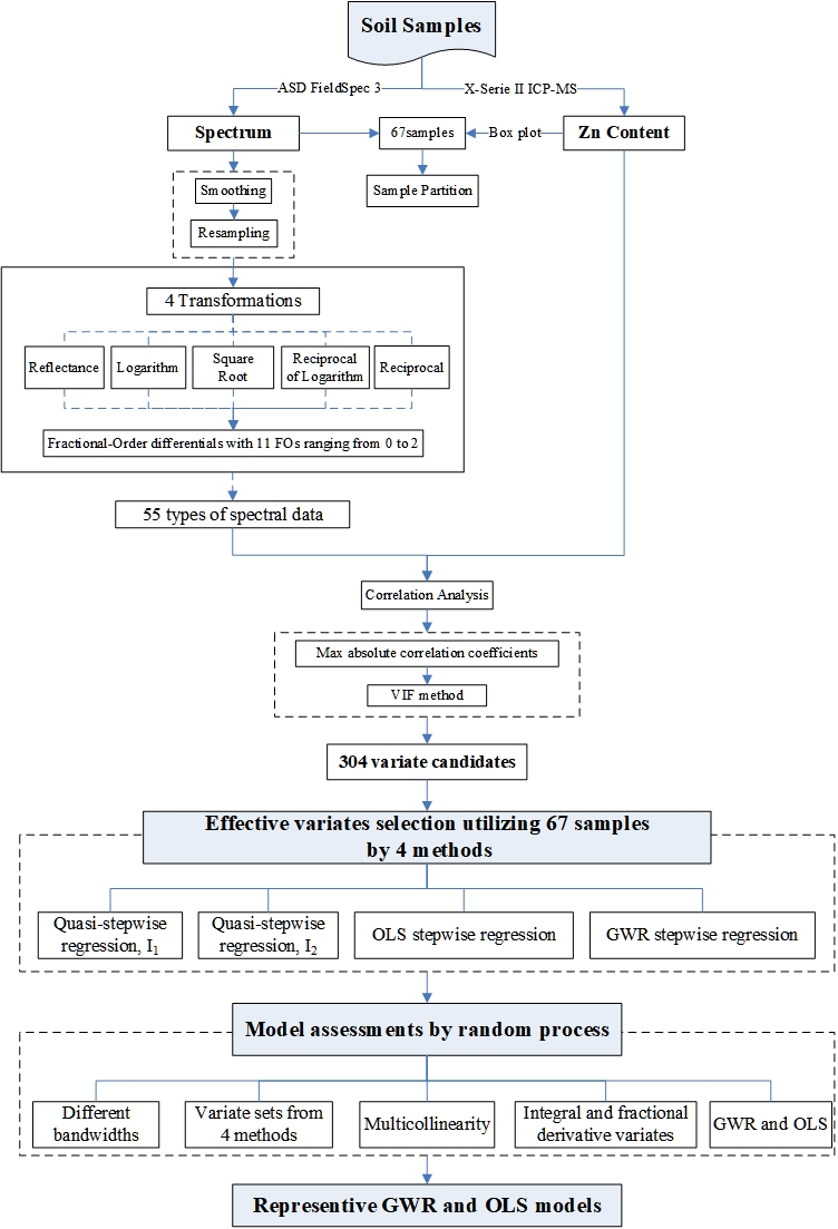
2. Materials and Methods
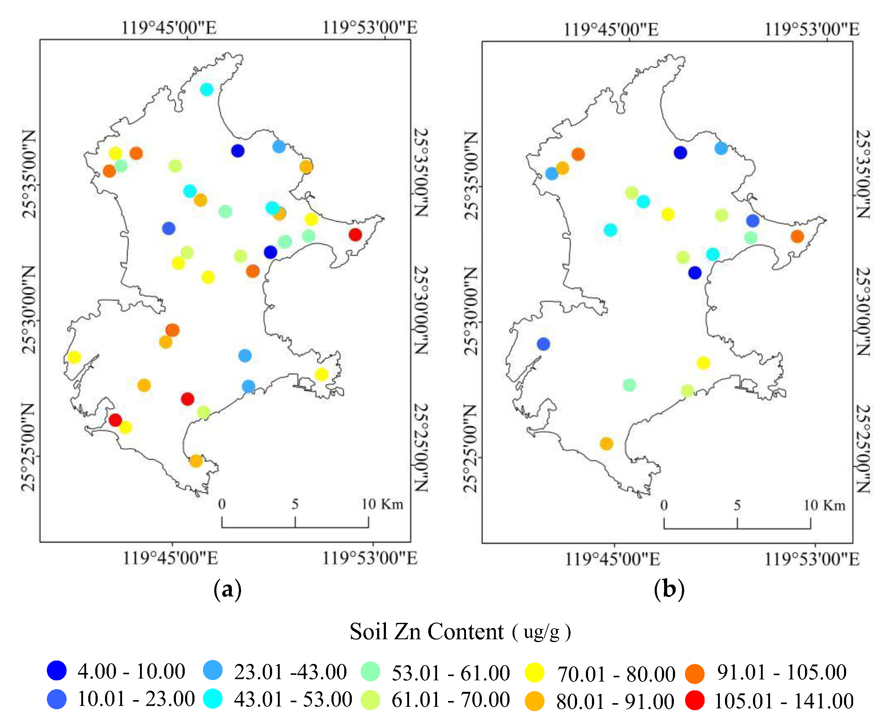
2.1. Study Site
2.2. Data Collection and Processing
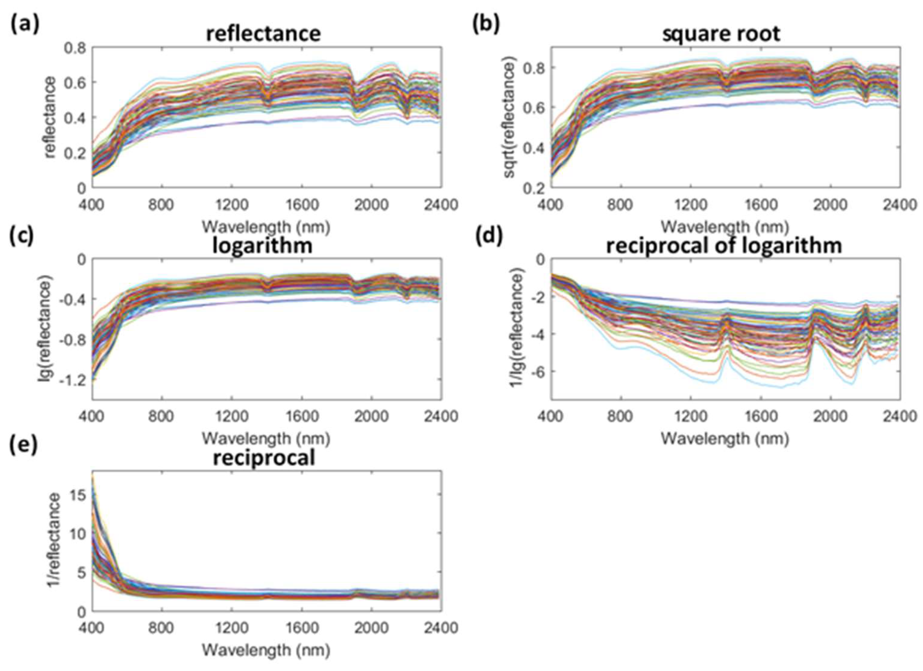
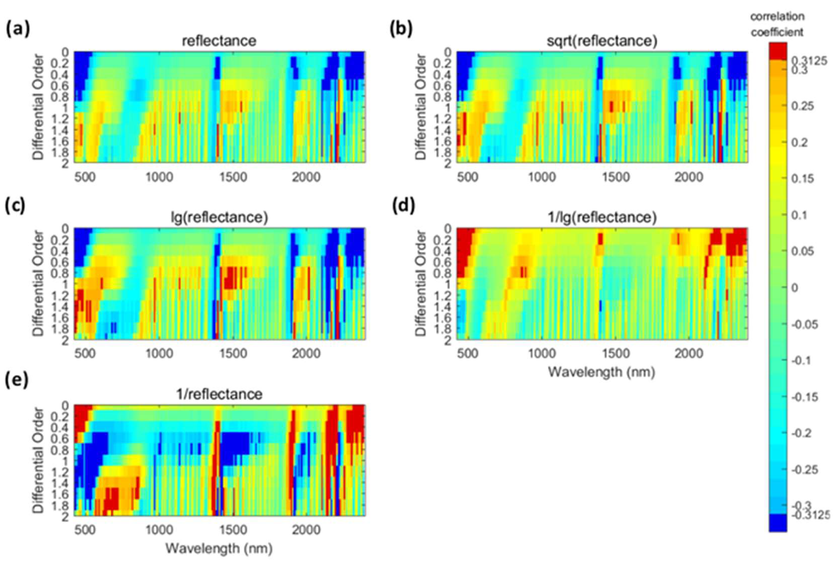
2.3. Data Transformations and Fractional-Order Differentials
2.4. Correlation Analyses and Data Sifting
2.5. Geographically Weighted Regression
3. Results and Discussion
3.1. Modeling Results of the 46 Samples
3.2. Variate Selections from 67 Samples
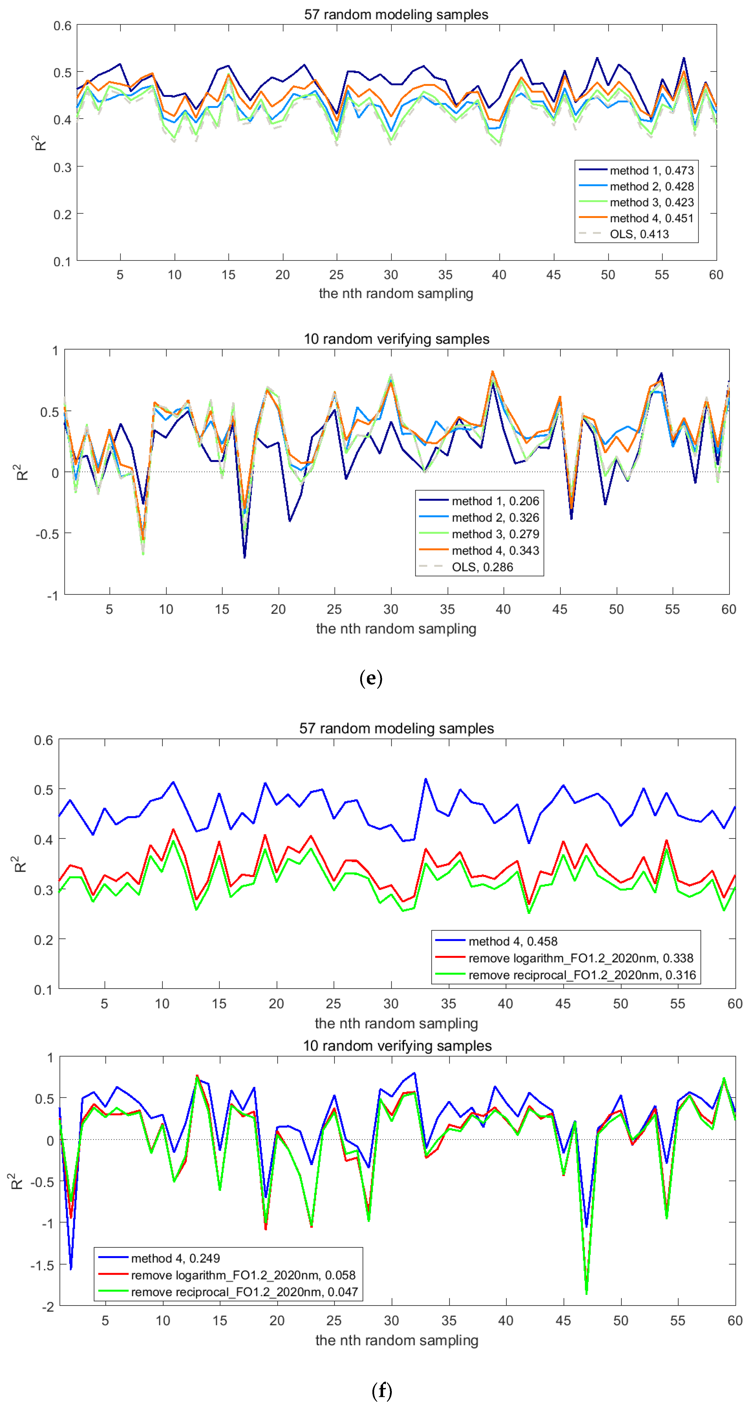
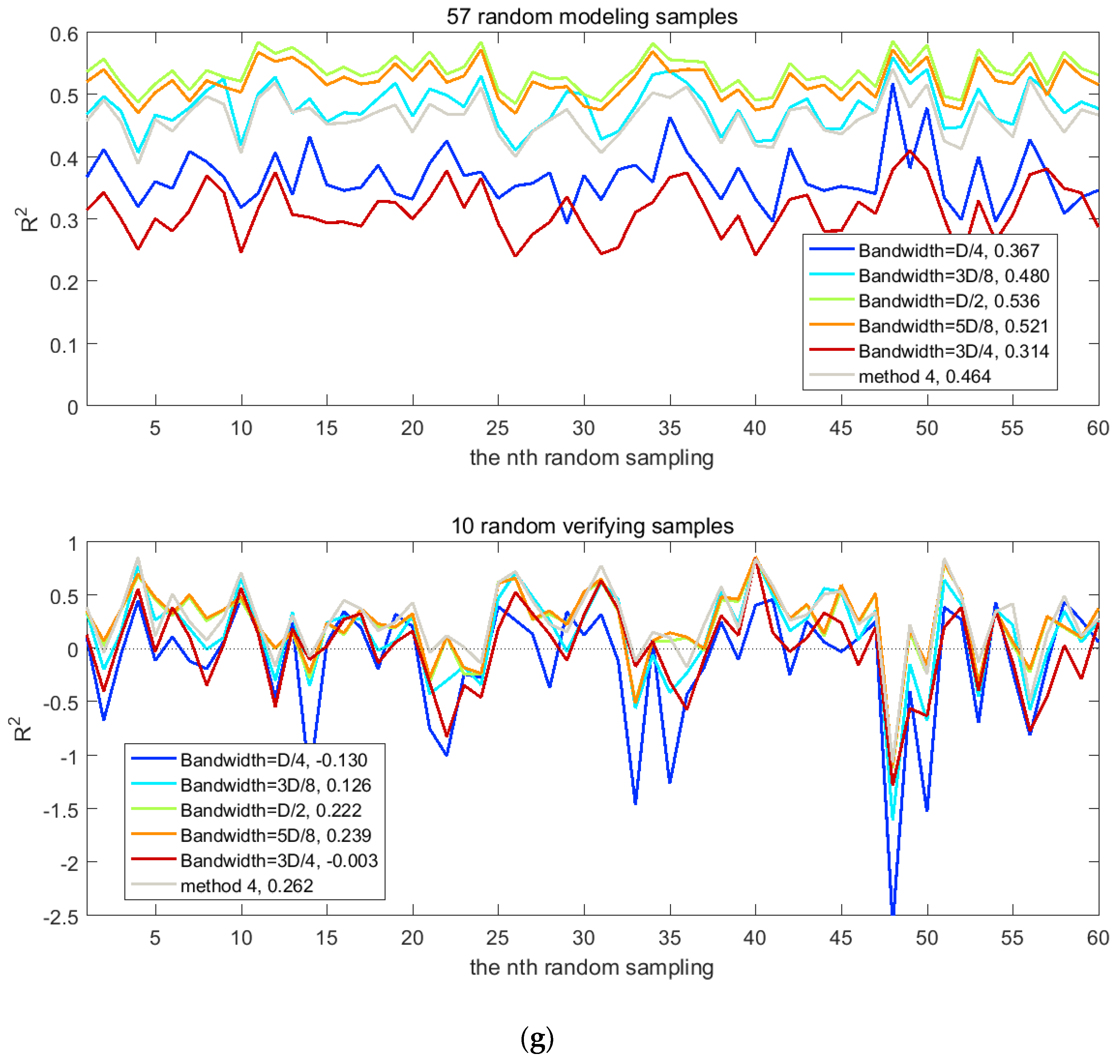
3.3. Model Assessments
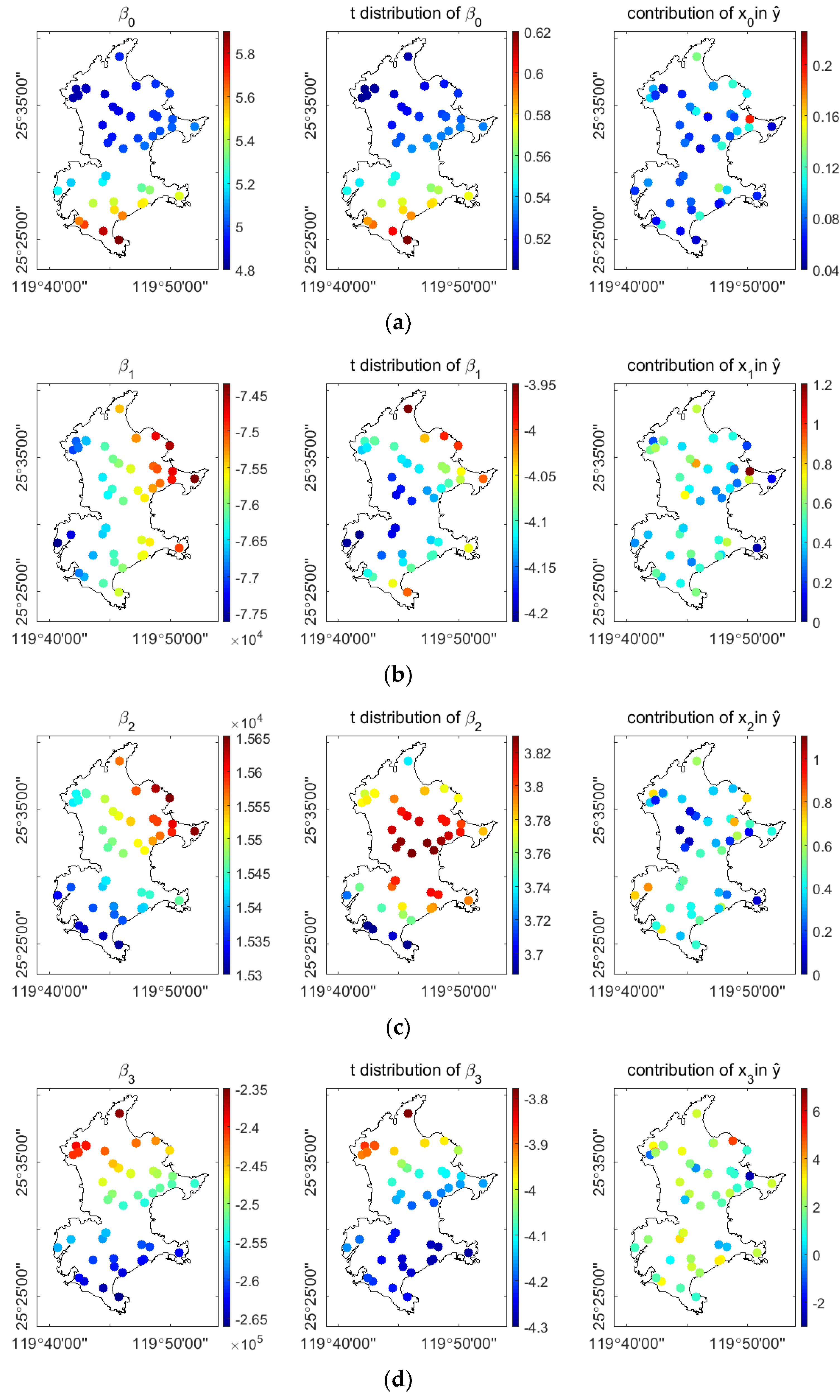
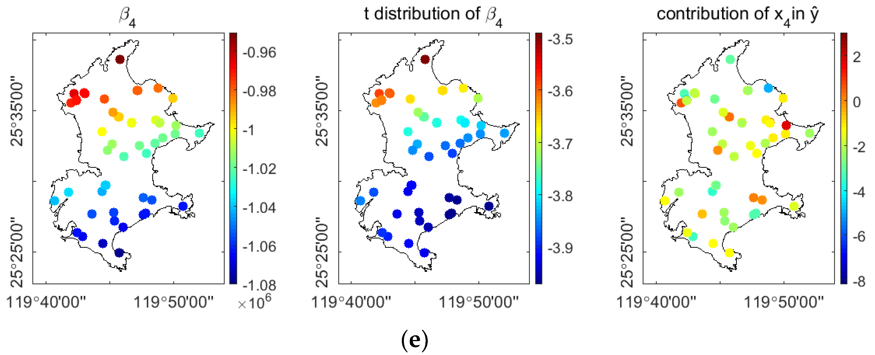
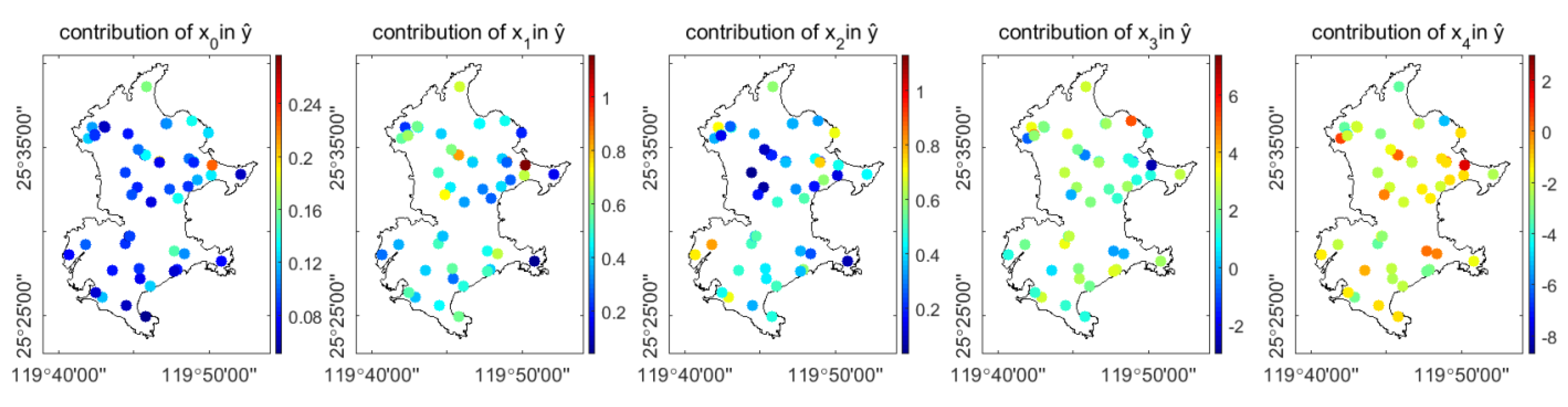
3.4. Analyses of Parameter Estimates
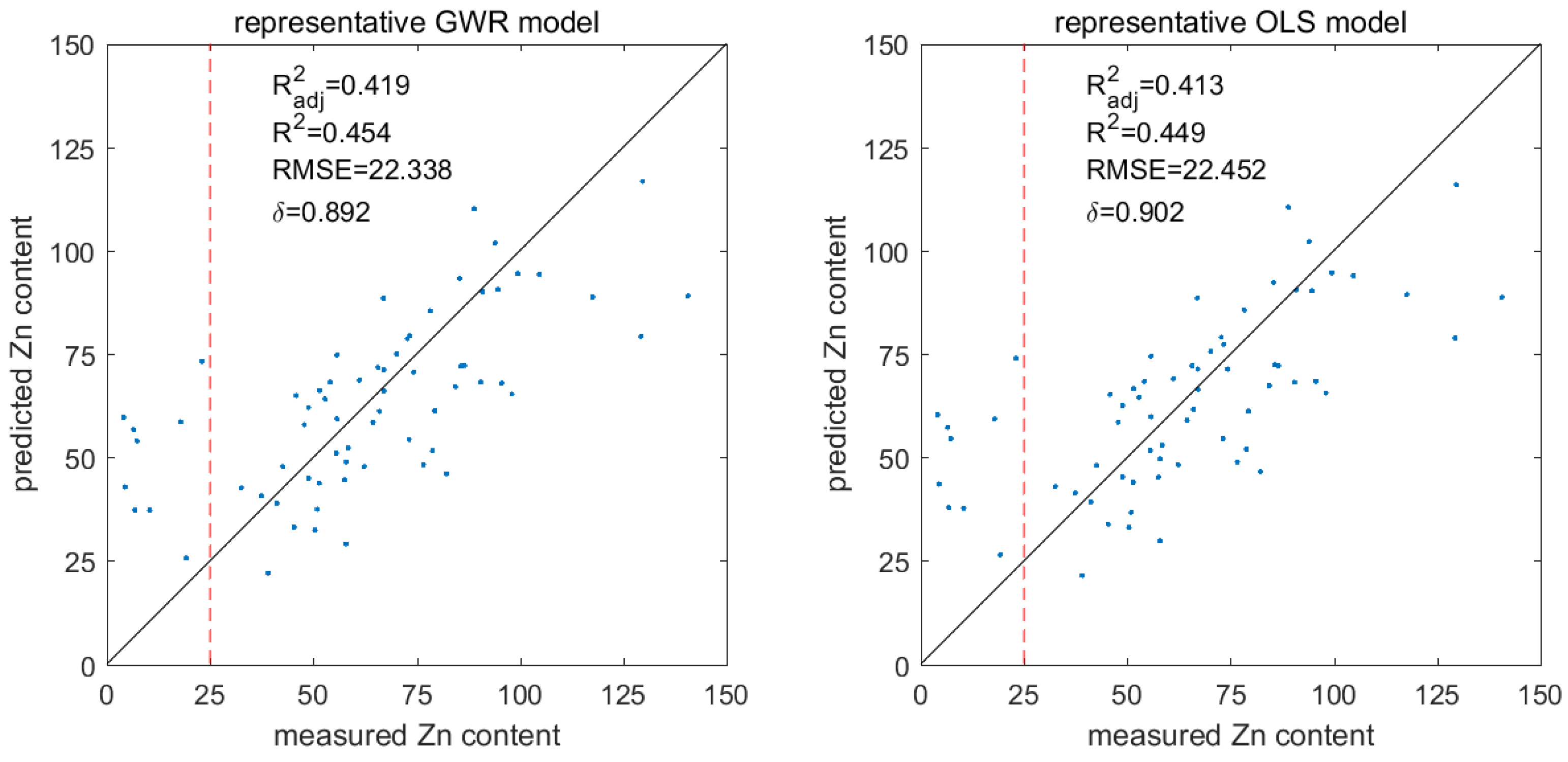
3.5. Performance of the Representative Models
3.6. Summary
4. Conclusions and Recommendations
Author Contributions
Funding
Acknowledgments
Conflicts of Interest
References
- He, J.; Zhang, S.; Zha, Y.; Jiang, J. Review of retrieving soil heavy metal content by hyperspectral remote sensing. Remote Sens. Technol. Appl. 2015, 30, 407–412. [Google Scholar] [CrossRef]
- Chi, G.; Guo, N.; Chen, X. Hyperspectral remote sensing monitoring on heavy metal contaminated farmland. Soils Crops 2017, 6, 243–250. [Google Scholar] [CrossRef]
- Wang, F.; Gao, J.; Zha, Y. Hyperspectral sensing of heavy metals in soil and vegetation: Feasibility and challenges. ISPRS J. Photogramm. Remote Sens. 2018, 136, 73–84. [Google Scholar] [CrossRef]
- Liu, J.; Dong, Z.; Sun, Z.; Ma, H.; Shi, L. Study on hyperspectral characteristics and estimation model of soil mercury content. IOP Conf. Ser. Mater. Sci. Eng. 2017, 274, 012030. [Google Scholar] [CrossRef]
- Wu, Y.Z.; Chen, J.; Ji, J.F.; Tian, Q.J.; Wu, X.M. Feasibility of reflectance spectroscopy for the assessment of soil mercury contamination. Environ. Sci. Technol. 2005, 39, 873–878. [Google Scholar] [CrossRef] [PubMed]
- Xia, F.; Peng, J.; Wang, Q.L.; Zhou, L.Q.; Shi, Z. Prediction of heavy metal content in soil of cultivated land: Hyperspectral technology at provincial scale. J. Infrared Millim. Waves 2015, 34, 593–598, 605. [Google Scholar] [CrossRef]
- Fotheringham, A.S.; Brunsdon, C.; Charlton, M. Geographically Weighted Regression: The Analysis of Spatially Varying Relationships; Wiley: Chichester, UK, 2002; ISBN 978-0-470-85525-6. [Google Scholar]
- Fotheringham, A.S.; Charlton, M.; Brunsdon, C. The geography of parameter space: An investigation of spatial non-stationarity. Int. J. Geogr. Inf. Syst. 1996, 10, 605–627. [Google Scholar] [CrossRef]
- Brunsdon, C.; Fotheringham, A.S.; Charlton, M.E. Geographically weighted regression: A method for exploring spatial nonstationarity. Geogr. Anal. 1996, 28, 281–298. [Google Scholar] [CrossRef]
- Jaber, S.M.; Al-Qinna, M.I. Global and local modeling of soil organic carbon using Thematic Mapper data in a semi-arid environment. Arab. J. Geosci. 2015, 8, 3159–3169. [Google Scholar] [CrossRef]
- Jiang, Z.; Yang, Y.; Sha, J. Application of GWR model in hyperspectral prediction of soil heavy metals. Acta Geogr. Sin. 2017, 72, 533–544. [Google Scholar] [CrossRef]
- Jiang, Z.L.; Yang, Y.S.; Sha, J.M. Study on GWR model applied for hyperspectral prediction of soil chromium in Fuzhou City. Acta Ecol. Sin. 2017, 37, 8117–8127. [Google Scholar] [CrossRef]
- Xu, J.; Feng, X.; Guan, L.; Wang, S.; Hu, Q. Fractional differential application in reprocessing infrared spectral data. Control Instrum. Chem. Ind. 2012, 39, 347–351. [Google Scholar] [CrossRef]
- Wang, J.; Tiyip, T.; Ding, J.; Zhang, D.; Liu, W.; Wang, F. Quantitative estimation of organic matter content in arid soil using Vis-NIR spectroscopy preprocessed by fractional derivative. J. Spectrosc. 2017, 2017, 1375158. [Google Scholar] [CrossRef]
- Wang, J.; Tiyip, T.; Zhang, D. Spectral detection of chromium content in desert soil based on fractional differential. Trans. Chin. Soc. Agric. Mach. 2017, 48, 152–158. [Google Scholar] [CrossRef]
- O’brien, R.M. A caution regarding rules of thumb for variance inflation factors. Qual. Quant. 2007, 41, 673–690. [Google Scholar] [CrossRef]
- Fotheringham, A.S.; Oshan, T.M. Geographically weighted regression and multicollinearity: Dispelling the myth. J. Geogr. Syst. 2016, 18, 303–329. [Google Scholar] [CrossRef]
- Standards Press of China. Classification and Codes for Chinese Soil; Standards Press of China: Beijing, China, 2009. [Google Scholar]
- Li, S.; Li, H.; Sun, D.; Zhou, L.; Bao, J. Characteristic and diagnostic bands of heavy metals in Beijing agricultural soils based on spectroscopy. Chin. J. Soil Sci. 2011, 42, 730–735. [Google Scholar] [CrossRef]
- Xie, X.; Sun, B.; Hao, H. Relationship between visible-near infrared reflectance spectroscopy and heavy metal of soil concentration. Acta Pedol. Sin. 2007, 44, 982–993. [Google Scholar] [CrossRef]
- Zhang, D.; Tiyip, T.; Zhang, F.; Kelimu, A.; Xia, N. Effect of fractional differential algorithm on hyperspectral data of saline soil. Acta Opt. Sin. 2016, 36, 0330002. [Google Scholar] [CrossRef]
- Chasco Yrigoyen, C.; García Rodríguez, I.; Vicéns Otero, J. Modeling spatial variations in household disposable income with geographically weighted regression(1). Estadística Española 2008, 50, 321–360. [Google Scholar]


| Heavy Metal Element | Min (mg/kg) | Max (mg/kg) | x (mg/kg) | SD (mg/kg) | cv (%) | Kurtosis | Skewness |
|---|---|---|---|---|---|---|---|
| Zn | 4 | 141 | 63.180 | 30.529 | 48.321 | 0.161 | 0.080 |
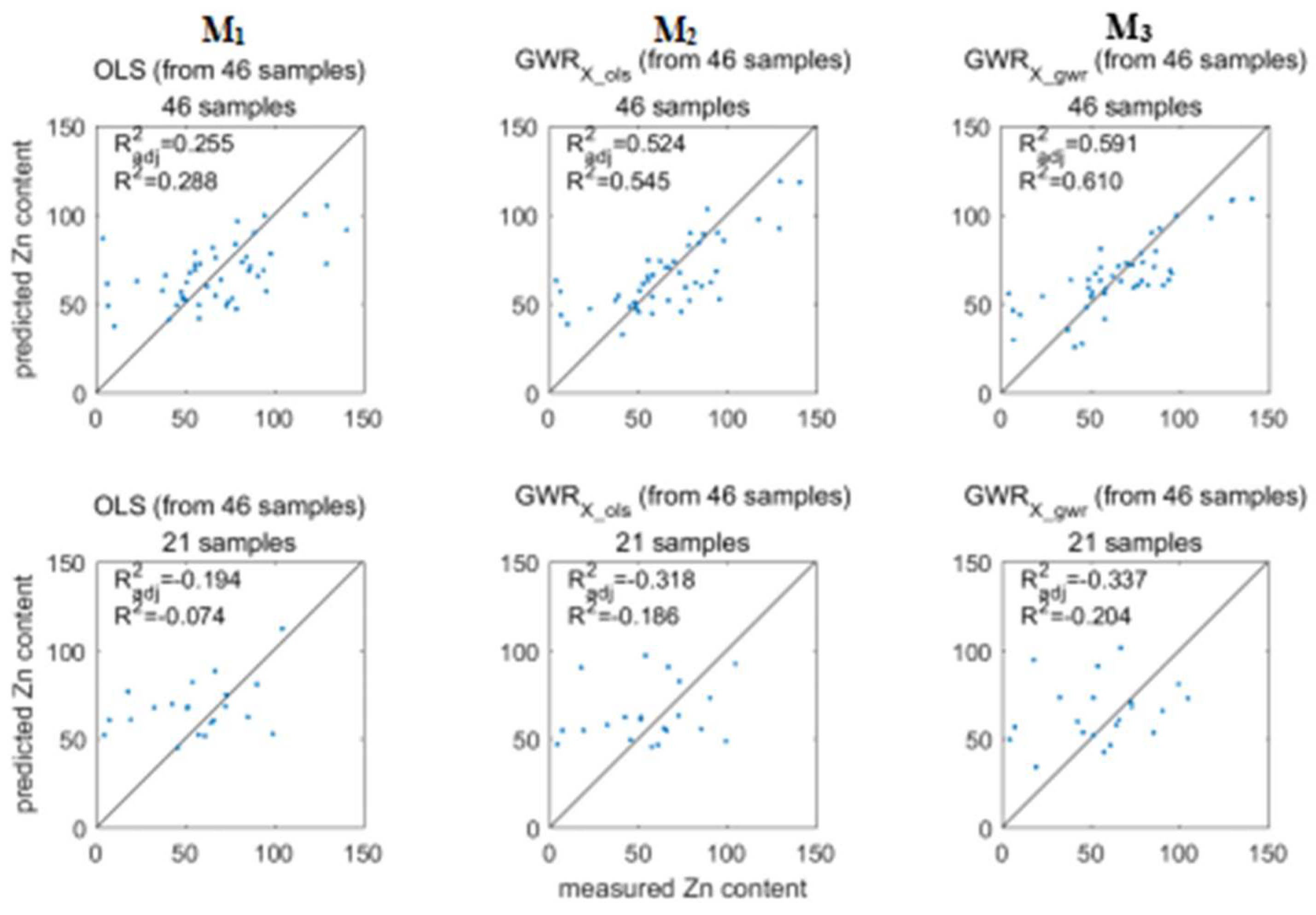
| M1 (OLS) | M2 (GWR) | M3 (GWR) | |||||
|---|---|---|---|---|---|---|---|
| D/4 | D/2 | 3D/4 | D/4 | D/2 | 3D/4 | ||
| Rm2 | 0.288 | 0.545 | 0.396 | 0.342 | 0.610 | 0.430 | 0.403 |
| Radj,m2 | 0.255 | 0.524 | 0.368 | 0.311 | 0.591 | 0.389 | 0.360 |
| Rv2 | –0.074 | –0.186 | –0.075 | –0.067 | –0.204 | –0.181 | –0.217 |
| Radj,v2 | –0.194 | –0.318 | –0.194 | –0.186 | –0.337 | –0.390 | –0.432 |
| x1 | reciprocal, FO = 0.8, 1560 nm | logarithm, FO = 1, 1140 nm | reciprocal, FO = 0.8, 1560 nm | ||||
| x2 | sqrt, FO = 1.2, 1140 nm | reciprocal, FO = 1, 2020 nm | reciprocal, FO = 0.8, 1010 nm | ||||
| x3 | reciprocal, FO = 0.6, 1010 nm | ||||||
| Bandwidth = D/4 | ||||
| Variates | I1 | tnew | Radj,m2 | Radj,v2 |
| reciprocal, FO = 1.6, 1510 nm | 0.0458 | 1.0826 | 0.2822 | 0.1498 |
| reciprocal, FO = 1.6, 1510 nm*; reciprocal, FO = 1, 1560 nm | 0.1421 | 1.8641 | 0.3916 | 0.1947 |
| reciprocal, FO = 1, 1560 nm; reciprocal, FO = 0.8, 2310 nm | 0.1634 | 1.743 | 0.4477 | 0.2094 |
| reciprocal, FO = 1, 1560 nm; reciprocal, FO = 0.8, 2310 nm*; reciprocal, FO = 0.8, 2020 nm | 0.1147 | 1.4718 | 0.4997 | 0.1559 |
| reciprocal, FO = 1, 1560 nm; reciprocal, FO = 0.8, 2020 nm; reciprocal, FO = 1.2, 970 nm | 0.0817 | 1.0291 | 0.5489 | 0.1446 |
| Bandwidth = D/2 | ||||
| Variates | I1 | tnew | Radj,m2 | Radj,v2 |
| logarithm, FO = 1, 1560 nm | 0.0236 | 2.6336 | 0.1794 | 0.0500 |
| logarithm, FO = 1, 1560 nm; reciprocal, FO = 2, 2200 nm | 0.0786 | 2.0766 | 0.2387 | 0.1587 |
| logarithm, FO = 1, 1560 nm; reciprocal, FO = 2, 2200 nm; sqrt, FO = 0.6, 1380 nm; | 0.0673 | 1.4093 | 0.2783 | 0.1717 |
| logarithm, FO = 1, 1560 nm; reciprocal, FO = 2, 2200 nm; sqrt, FO = 0.6, 1380 nm; reciprocal, FO = 1, 2200 nm | 0.1106 | 2.0686 | 0.3555 | 0.1504 |
| logarithm, FO = 1, 1560 nm; reciprocal, FO = 2, 2200 nm; sqrt, FO = 0.6, 1380 nm; reciprocal, FO = 1, 2200 nm; logarithm, FO = 1, 2200 nm | 0.0754 | 1.6947 | 0.3979 | 0.1119 |
| logarithm, FO = 1, 1560 nm; reciprocal, FO = 2, 2200 nm; sqrt, FO = 0.6, 1380 nm*; reciprocal, FO = 1, 2200 nm; logarithm, FO = 1, 2200 nm; reciprocal of logarithm, FO = 0.2, 1930 nm | 0.0659 | 1.0264 | 0.4062 | 0.1580 |
| logarithm, FO = 1, 1560 nm; reciprocal, FO = 2, 2200 nm; reciprocal, FO = 1, 2200 nm; logarithm, FO = 1, 2200 nm; reciprocal of logarithm, FO = 0.2, 1930 nm; logarithm, FO = 1.6, 2170 nm | 0.0885 | 1.1712 | 0.4224 | 0.1790 |
| Bandwidth = 3D/4 | ||||
| Variates | I1 | tnew | Radj,m2 | Radj,v2 |
| reciprocal, FO = 0.8, 2220 nm | 0.0160 | 2.6938 | 0.1473 | 0.0404 |
| reciprocal, FO = 0.8, 2220 nm; reciprocal, FO = 1, 1560 nm | 0.0525 | 2.1102 | 0.2116 | 0.1176 |
| reciprocal, FO = 0.8, 2220 nm; reciprocal, FO = 1, 1560 nm; sqrt, FO = 0.6, 1380 nm | 0.0399 | 1.2801 | 0.2269 | 0.1374 |
| reciprocal, FO = 0.8, 2220 nm; reciprocal, FO = 1, 1560 nm; sqrt, FO = 0.6, 1380 nm; reciprocal, FO = 1.2, 2020 nm | 0.0669 | 1.8941 | 0.2791 | 0.1265 |
| reciprocal, FO = 0.8, 2220 nm; reciprocal, FO = 1, 1560 nm; sqrt, FO = 0.6, 1380 nm; reciprocal, FO = 1.2, 2020 nm; logarithm, FO = 1.2, 2020 nm | 0.1016 | 1.8254 | 0.3257 | 0.1709 |
| reciprocal, FO = 0.8, 2220 nm*; reciprocal, FO = 1, 1560 nm; sqrt, FO = 0.6, 1380 nm *; reciprocal, FO = 1.2, 2020 nm; logarithm, FO = 1.2, 2020 nm; reciprocal of logarithm, FO = 1.8, 2200 nm | 0.0918 | 2.1128 | 0.3804 | 0.1143 |
| reciprocal, FO = 1, 1560 nm; reciprocal, FO = 1.2, 2020 nm; logarithm, FO = 1.2, 2020 nm; reciprocal of logarithm, FO = 1.8, 2200 nm; logarithm, FO = 1.8, 700 nm | 0.0827 | 1.4927 | 0.4124 | 0.1343 |
| Bandwidth = D/4 | |||||
| Variates | I2 | tnew | tmin | Radj,m2 | Radj,v2 |
| reciprocal, FO = 1, 1560 nm | 0.0174 | 1.9250 | 0.6434 | 0.3303 | 0.0424 |
| reciprocal, FO = 1, 1560 nm; reciprocal, FO = 2, 640 nm | 0.0415 | 1.8741 | 0.3729 | 0.4261 | 0.1395 |
| reciprocal, FO = 1, 1560 nm; reciprocal, FO = 2, 640 nm; reciprocal of logarithm, FO = 2, 2200 nm | 0.0179 | 1.3117 | 0.2945 | 0.4441 | 0.1041 |
| reciprocal, FO = 1, 1560 nm; reciprocal, FO = 2, 640 nm; reciprocal of logarithm, FO = 2, 2200 nm; logarithm, FO = 0.6, 2380 nm | 0.0076 | 1.1330 | 0.1056 | 0.5363 | 0.1182 |
| reciprocal, FO = 1, 1560 nm; reciprocal, FO = 2, 640 nm; reciprocal of logarithm, FO = 2, 2200 nm; logarithm, FO = 0.6, 2380 nm; reciprocal, FO = 1.8, 820 nm | 0.0125 | 1.3054 | 0.0673 | 0.6454 | 0.2198 |
| reciprocal, FO = 1, 1560 nm; reciprocal, FO = 2, 640 nm; reciprocal of logarithm, FO = 2, 2200 nm; logarithm, FO = 0.6, 2380 nm; reciprocal, FO = 1.8, 820 nm; reciprocal, FO = 1.2, 1970 nm | 0.1091 | 1.6182 | 0.7625 | 0.6897 | 0.1281 |
| Bandwidth = D/2 | |||||
| Variates | I2 | tnew | tmin | Radj,m2 | Radj,v2 |
| logarithm, FO = 1, 1560 nm | 0.0505 | 2.6336 | 2.1384 | 0.1794 | 0.05 |
| logarithm, FO = 1, 1560 nm; logarithm, FO = 2, 2200 nm; | 0.1249 | 2.1617 | 1.6863 | 0.2399 | 0.1428 |
| logarithm, FO = 1, 1560 nm; logarithm, FO = 2, 2200 nm; reflectance, FO = 1, 1560 nm | 0.064 | 1.9158 | 1.5799 | 0.2943 | 0.0719 |
| logarithm, FO = 1, 1560 nm; logarithm, FO = 2, 2200 nm; reflectance, FO = 1, 1560 nm; reciprocal, FO = 1.2, 2020 nm | 0.0467 | 1.7515 | 1.2311 | 0.3474 | 0.0623 |
| logarithm, FO = 1, 1560 nm; logarithm, FO = 2, 2200 nm; reflectance, FO = 1, 1560 nm; reciprocal, FO = 1.2, 2020 nm; logarithm, FO = 1.2, 2020 nm | 0.0410 | 1.1916 | 0.8381 | 0.3508 | 0.1170 |
| Bandwidth = 3D/4 | |||||
| Variates | I2 | tnew | tmin | Radj,m2 | Radj,v2 |
| reciprocal, FO = 0.8, 2220 nm | 0.0405 | 2.6938 | 2.5271 | 0.1473 | 0.0404 |
| reciprocal, FO = 0.8, 2220 nm; reciprocal, FO = 1, 1560 nm | 0.1010 | 2.1102 | 1.9241 | 0.2116 | 0.1176 |
| reciprocal, FO = 0.8, 2220 nm*; reciprocal, FO = 1, 1560 nm; reciprocal, FO = 1.2, 2020 nm | 0.0578 | 1.8003 | 1.5415 | 0.2590 | 0.0804 |
| reciprocal, FO = 1, 1560 nm; reciprocal, FO = 1.2, 2020 nm; reciprocal of logarithm, FO = 2, 2200 nm | 0.1100 | 2.0887 | 1.9006 | 0.3049 | 0.0909 |
| reciprocal, FO = 1, 1560 nm; reciprocal, FO = 1.2, 2020 nm; reciprocal of logarithm, FO = 2, 2200 nm; logarithm, FO = 1.2, 2020 nm | 0.2670 | 2.1087 | 1.8366 | 0.3591 | 0.1920 |
| reciprocal, FO = 1, 1560 nm; reciprocal, FO = 1.2, 2020 nm; reciprocal of logarithm, FO = 2, 2200 nm; logarithm, FO = 1.2, 2020 nm; logarithm, FO = 1.8, 680 nm | 0.1119 | 2.1072 | 1.7310 | 0.4132 | 0.0742 |
| reciprocal, FO = 1, 1560 nm; reciprocal, FO = 1.2, 2020 nm; reciprocal of logarithm, FO = 2, 2200 nm; logarithm, FO = 1.2, 2020 nm; logarithm, FO = 1.8, 680 nm; reciprocal of logarithm, FO = 0.4, 2140 nm | 0.0141 | 1.1922 | 1.0272 | 0.4263 | 0.0269 |
| reciprocal, FO = 1, 1560 nm; reciprocal, FO = 1.2, 2020 nm; reciprocal of logarithm, FO = 2, 2200 nm; logarithm, FO = 1.2, 2020 nm; logarithm, FO = 1.8, 680 nm; reciprocal of logarithm, FO = 0.4, 2140 nm; reciprocal, FO = 0.8, 1010 nm | 0.0204 | 1.3752 | 1.2141 | 0.4493 | 0.0271 |
| Method 1 (46 samples) | variates | reciprocal, FO = 1, 1560 nm; | reciprocal, FO = 0.8, 2310 nm | ||
| t | 1.657 | 1.743 | |||
| tmin | 0.119 | 0.001 | |||
| Method 1 (67 samples) | t | 2.305 | 2.312 | ||
| tmin | 0.142 | 0.060 | |||
| Method 2 (46 samples) | variates | reciprocal, FO = 1, 1560 nm | reciprocal, FO = 1.2, 2020 nm | reciprocal of logarithm, FO = 2, 2200 nm | logarithm, FO = 1.2, 2020 nm |
| t | 2.458 | 2.396 | 2.607 | 2.109 | |
| tmin | 2.234 | 2.101 | 2.449 | 1.837 | |
| Method 2 (67 samples) | t | 3.682 | 3.345 | 3.364 | 3.002 |
| tmin | 3.507 | 2.927 | 3.212 | 2.589 | |
| Method 3 (67 samples) | variates | reciprocal, FO = 0.8, 1560 nm | reciprocal, FO = 1.2, 2020 nm | logarithm, FO = 1.2, 2020 nm | reciprocal of logarithm, FO = 1.6, 2200 nm |
| t | 3.479 | 4.166 | 3.889 | 2.467 | |
| tmin | 3.219 | 3.938 | 3.667 | 2.405 | |
| OLS (67 samples) | t | −3.558 | −4.272 | −4.001 | 2.607 |
| Bandwidth | Variates | Rm2 | Radj,m2 |
|---|---|---|---|
| D/4 | reciprocal, FO = 0.8, 2020 nm | 0.3673 | 0.3576 |
| 3D/8 | reciprocal, FO = 1, 1560 nm; reciprocal of logarithm, FO = 2, 2200 nm; reciprocal, FO = 1.2, 2020 nm; logarithm, FO = 1.2, 2020 nm | 0.4644 | 0.4299 |
| D/2 | reciprocal, FO = 1, 1560 nm; reciprocal of logarithm, FO = 1.6, 2200 nm; reciprocal, FO = 1.2, 2020 nm; logarithm, FO = 1.2, 2020 nm | 0.4634 | 0.4288 |
| 5D/8 | reciprocal, FO = 1, 1560 nm; reciprocal of logarithm, FO = 1.6, 2200 nm; reciprocal, FO = 1.2, 2020 nm; logarithm, FO = 1.2, 2020 nm | 0.4572 | 0.4221 |
| 3D/4 | reciprocal, FO = 1, 1560 nm; reciprocal of logarithm, FO = 1.6, 2200 nm; reciprocal, FO = 1.2, 2020 nm; logarithm, FO = 1.2, 2020 nm | 0.4542 | 0.4190 |
| Bandwidth | Variates | Rm2 | Radj,m2 |
|---|---|---|---|
| D/4 | reciprocal, FO = 1, 2020 nm | 0.337 | 0.326 |
| 3D/8 | reciprocal, FO = 1, 2020 nm; reciprocal, FO = 1, 1560 nm; reciprocal of logarithm, FO = 2, 2200 nm; logarithm, FO = 1, 2020 nm | 0.457 | 0.422 |
| D/2 | reciprocal, FO = 1, 2020 nm; reciprocal, FO = 1, 1560 nm; reciprocal of logarithm, FO = 2, 2200 nm; logarithm, FO = 1, 2020 nm; reciprocal of logarithm, FO = 0, 2200 nm; sqrt, FO = 2, 640 nm | 0.518 | 0.469 |
| 5D/8 | reciprocal, FO = 1, 2020 nm; reciprocal, FO = 1, 1560 nm; reciprocal of logarithm, FO = 2, 2200 nm; logarithm, FO = 1, 2020 nm; reciprocal of logarithm, FO = 0, 2200 nm; sqrt, FO = 2, 640 nm | 0.506 | 0.456 |
| 3D/4 | reciprocal, FO = 2, 2200 nm; reciprocal, FO = 1, 1560 nm; | 0.294 | 0.272 |
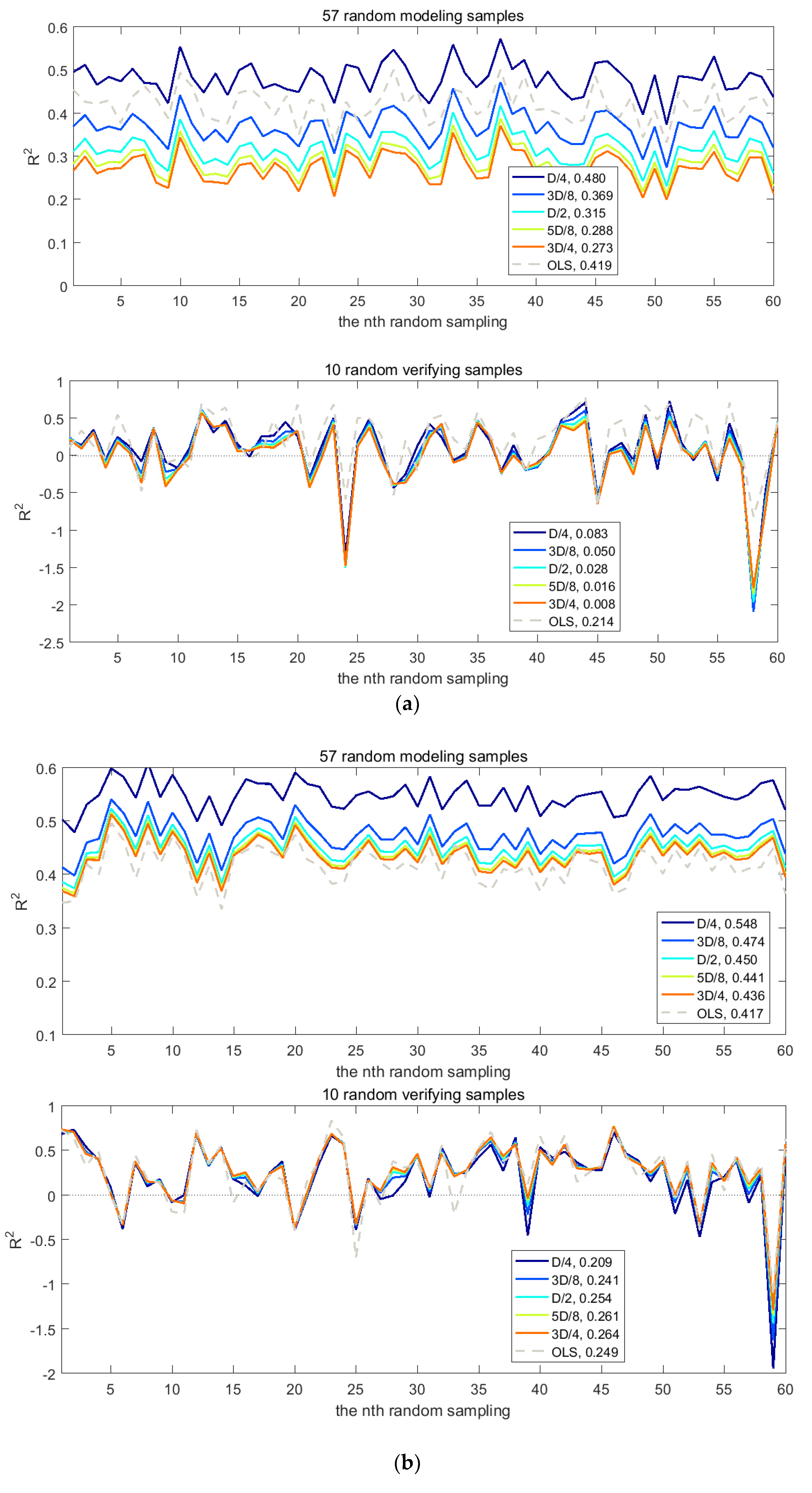
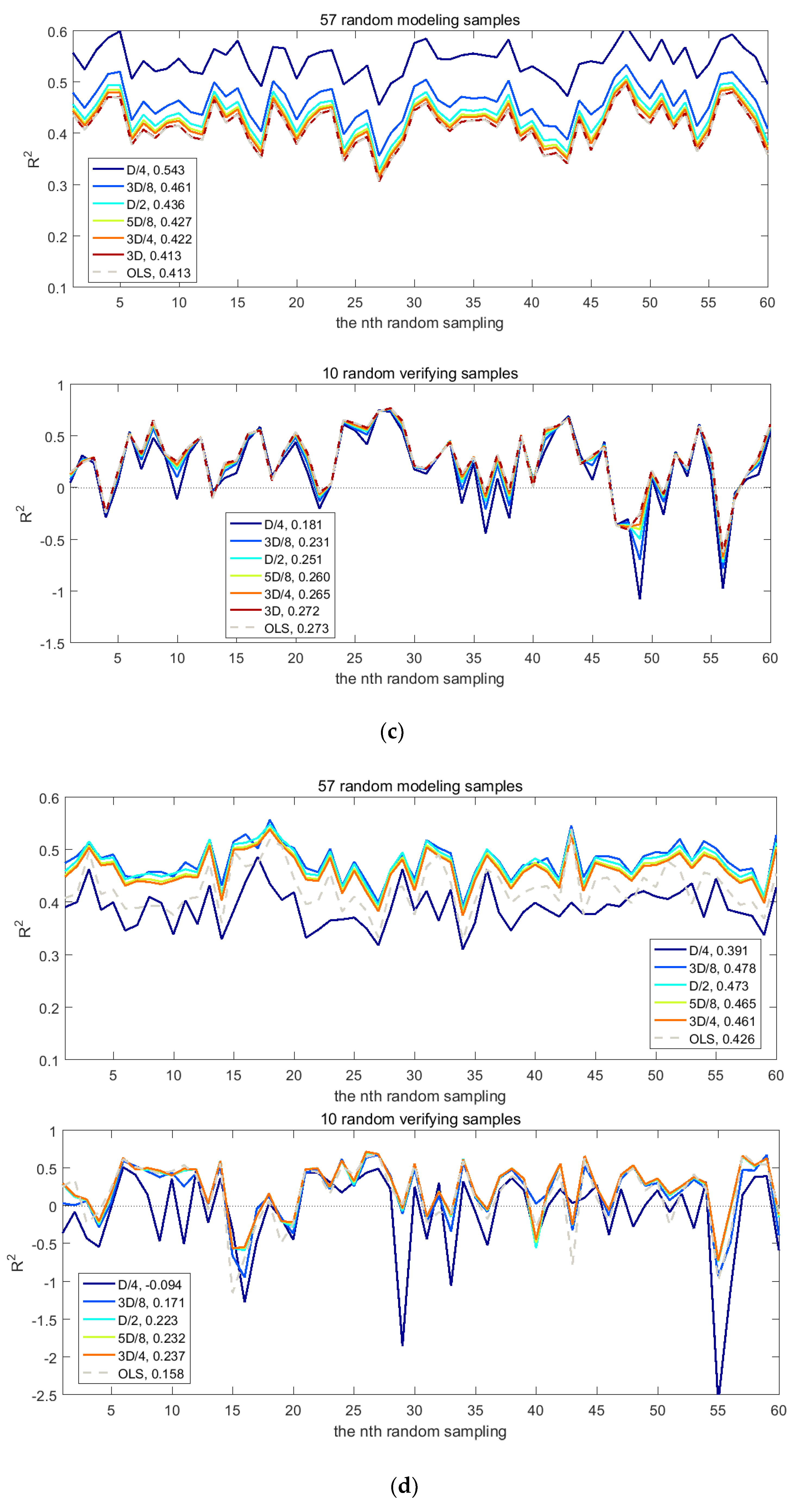
| Method 1 (D/4) | Method 2 (3D/4) | Method 3 (3D/4) | Method 4 (3D/4) | OLS | IO (5D/8) | IO (3D/4) | OLS-2 | OLS-3 | |
|---|---|---|---|---|---|---|---|---|---|
| Mean Rm2 | 0.480 | 0.438 | 0.432 | 0.459 | 0.423 | 0.519 | 0.510 | 0.452 | 0.488 |
| Mean Radj,m2 | 0.461 | 0.395 | 0.389 | 0.418 | 0.378 | 0.461 | 0.451 | 0.410 | 0.427 |
| Mean Rv2 | 0.082 | 0.205 | 0.163 | 0.242 | 0.175 | 0.220 | 0.228 | 0.253 | 0.244 |
| Mean Radj,v2 | −0.180 | −0.431 | −0.508 | −0.364 | −0.486 | −1.340 | −1.316 | −0.346 | −1.270 |
| Parameter | β0 | β1 | β2 | β3 | β4 |
|---|---|---|---|---|---|
| β | 5.922 | –7.460 × 10⁴ | 1.551 × 10⁴ | –2.515 × 10⁵ | –1.018 × 10⁶ |
| SE | 9.264 | 1.799 × 10⁴ | 3.989 × 10³ | 5.961 × 10⁴ | 2.604 × 10⁵ |
| t-value | 0.639 | −4.148 | 3.888 | −4.219 | −3.909 |
| Representative GWR model | Representative OLS model | |||||
|---|---|---|---|---|---|---|
| 67 samples | 9 samples (<25 mg/kg) | 58 samples (>25 mg/kg) | 67 samples | 9 samples (<25 mg/kg) | 58 samples (>25 mg/kg) | |
| Radj2 | 0.419 | –73.868 | 0.396 | 0.413 | –76.057 | 0.399 |
| R2 | 0.454 | –36.434 | 0.438 | 0.449 | –37.529 | 0.441 |
| RMSE | 22.338 | 40.977 | 17.773 | 22.452 | 41.571 | 17.725 |
| δ | 89.2% | 537.2% | 19.7% | 90.2% | 545.2% | 19.6% |
© 2019 by the authors. Licensee MDPI, Basel, Switzerland. This article is an open access article distributed under the terms and conditions of the Creative Commons Attribution (CC BY) license (http://creativecommons.org/licenses/by/4.0/).
Share and Cite
Lin, X.; Su, Y.-C.; Shang, J.; Sha, J.; Li, X.; Sun, Y.-Y.; Ji, J.; Jin, B. Geographically Weighted Regression Effects on Soil Zinc Content Hyperspectral Modeling by Applying the Fractional-Order Differential. Remote Sens. 2019, 11, 636. https://0-doi-org.brum.beds.ac.uk/10.3390/rs11060636
Lin X, Su Y-C, Shang J, Sha J, Li X, Sun Y-Y, Ji J, Jin B. Geographically Weighted Regression Effects on Soil Zinc Content Hyperspectral Modeling by Applying the Fractional-Order Differential. Remote Sensing. 2019; 11(6):636. https://0-doi-org.brum.beds.ac.uk/10.3390/rs11060636
Chicago/Turabian StyleLin, Xue, Yung-Chih Su, Jiali Shang, Jinming Sha, Xiaomei Li, Yang-Yi Sun, Jianwan Ji, and Biao Jin. 2019. "Geographically Weighted Regression Effects on Soil Zinc Content Hyperspectral Modeling by Applying the Fractional-Order Differential" Remote Sensing 11, no. 6: 636. https://0-doi-org.brum.beds.ac.uk/10.3390/rs11060636