Land Surface Temperature Retrieval from Sentinel-3A Sea and Land Surface Temperature Radiometer, Using a Split-Window Algorithm

Abstract

Land surface temperature (LST) is a crucial parameter in the interaction between the ground and the atmosphere. The Sentinel-3A Sea and Land Surface Temperature Radiometer (SLSTR) provides global daily coverage of day and night observation in the wavelength range of 0.55 to 12.0 μm. LST retrieved from SLSTR is expected to be widely used in different fields of earth surface monitoring. This study aimed to develop a split-window (SW) algorithm to estimate LST from two-channel thermal infrared (TIR) and one-channel middle infrared (MIR) images of SLSTR observation. On the basis of the conventional SW algorithm, using two TIR channels for the daytime observation, the MIR data, with a higher atmospheric transmittance and a lower sensitivity to land surface emissivity, were further used to develop a modified SW algorithm for the nighttime observation. To improve the retrieval accuracy, the algorithm coefficients were obtained in different subranges, according to the view zenith angle, column water vapor, and brightness temperature. The proposed algorithm can theoretically estimate LST with an error lower than 1 K on average. The algorithm was applied to northern China and southern UK, and the retrieved LST captured the surface features for both daytime and nighttime. Finally, ground validation was conducted over seven sites (four in the USA and three in China). Results showed that LST could be estimated with an error mostly within 1.5 to 2.5 K from the algorithm, and the error of the nighttime algorithm involved with MIR data was about 0.5 K lower than the daytime algorithm.

1. Introduction

Land surface temperature (LST), which is the key parameter in the interaction between the ground and the atmosphere, plays a significant role in the fields of agriculture, meteorology, ecology, and hydrology [1,2]. LST has a complex spatial and temporal distribution, due to the changing surface type and atmospheric conditions. Therefore, ground measurements cannot practically provide LST values at a large scale. Remote sensing data offer the only possibility of measuring LST around the globe with sufficiently high spatial and temporal resolution [3].

LST retrieval from remote sensing data can be traced back to the 1970s [4]. Many LST retrieval methods have been proposed for thermal infrared (TIR) data under different assumptions of atmosphere and emissivity in order to solve the problems identified when calculating LST from satellite data, as follows: Atmospheric correction from the sensor to the ground and the impact of land surface emissivity (LSE) [5]. Among all of these methods, the split-window (SW) algorithm is one of the most effective and widely used methods. The conventional SW algorithm utilizes linear or nonlinear combinations of the brightness temperature at the top of the atmosphere (TOA) of two adjacent TIR channels at around 11 and 12 μm to remove the atmospheric effect during radiative transfer and to estimate LST. It has been applied to retrieve LST from various sensors, such as Moderate Resolution Imaging Spectroradiometer (MODIS), Landsat 8, and Chinese FengYun-2C (FY-2C) [6,7,8]. On the basis of the conventional SW algorithm, if more than two TIR bands are available on the sensor, new forms of SW algorithms can be developed to make full use of the spectral information. For instance, Ye et al. [9] proposed a four-channel algorithm and applied it to Chinese Gaofen-5 (GF-5) satellite data. Sun and Pinker [10] proposed a three-channel algorithm that could be applied to any sensor with three TIR channels. Results show that multichannel algorithms provide a more accurate retrieval than conventional ones.

It is known that middle infrared (MIR) data, which also contain the thermal radiance information of land surface, according to the Planck’s law, can be used for LST retrieval. Moreover, MIR channels have lower atmospheric absorption and attenuation than TIR channels [10]. However, retrieving LST from MIR data is challenging and therefore not as developed as retrieval from TIR, because MIR data contain reflected solar irradiance during the daytime, which is difficult to separate from the land surface thermal radiance. MIR data observed at night can be used to retrieve LST because it does not contain solar irradiance. For instance, Zhao et al. [11] applied the SW algorithm to nighttime MIR observation and developed a modified algorithm for retrieving LST from two-channel MIR data at night. On the basis of this study, Zhao et al. [12] further proposed a method to estimate the solar irradiance during the daytime and established a new LST retrieval algorithm from daytime MIR data.

The European Commission Sentinels are a fleet of satellites designed to deliver the wealth of data and imagery that are central to the European Commission’s Copernicus program. Among all the satellites, Sentinel-3A was launched on 16 February 2016 and flies at an altitude of 814.5 km at a near-polar, sun-synchronous orbit with a descending node equatorial crossing at 10:00 of the mean local solar time [13]. It carries the Sea and Land Surface Temperature Radiometer (SLSTR), which follows on from the previous Along Track Scanning Radiometers (ATSR) series in terms of measuring the surface temperature of the earth. SLSTR observes the global surface daily in nine bands, of which three are in visible and near infrared ranges (VNIR, centered at 0.555, 0.659, and 0.865 μm), three are in short wave infrared ranges (SWIR, centered at 1.375, 1.610, and 2.25 μm), and three are in middle and thermal infrared ranges (MIR/TIR, centered at 3.74, 10.85, and 12.0 μm). Both VNIR and SWIR images are captured at a resolution of 0.5 km, whereas both MIR and TIR images are captured at a resolution of 1 km. The two TIR channels and one MIR channel on the SLSTR are designed to maintain a highly accurate earth surface temperature, but up to now, no publications about the LST retrieval algorithm and validation from those data are available. The existing SLSTR LST product only utilizes the two TIR channels using a nadir-only split-window algorithm based on a regression coefficient approach that relies on statistics to generate realistic retrieval coefficients, but the MIR channel observation is still not fully used. Moreover, the existing product directly puts water vapor and view zenith angle into the algorithm equation as parameters, which may make the retrieval result more sensitive to the error of water vapor and view zenith angle [14,15]. Therefore, it is necessary to develop and report a specified algorithm to retrieve LST from Sentinel-3A SLSTR by fully using the MIR and TIR data and reduce the sensitivity to the uncertainty of other auxiliary parameters. From this point of view, the study is the first to focus on this topic on the basis of the split-window algorithm. Sentinel-3B was launched on 25 April 2018 and has the same channel specification as Sentinel-3A. Thus, the LST algorithms developed in this paper will also be useful for Sentinel-3B. As a result, this study will be organized as follows: Section 2 presents the development of the new SW algorithm and the method to obtain the necessary parameters for LST retrieval. Section 3 shows the application of the proposed algorithm and its validation results, using ground-measured data. Finally, Section 4 presents discussions and conclusions.

2. Methodology

2.1. Theoretical Background

According to the thermal radiative transfer model, for a cloud-free atmosphere under local thermodynamic equilibrium, the thermal radiance observed at the TOA can be expressed as [3]

$$L_i=[{\epsilon }_i{B}_i\left(T_s\right)+\left(1-{\epsilon }_i\right)R_{ai}^{\downarrow }]{\tau }_i+R_{ai}^{\uparrow }$$

(1)

where ε_i is the emissivity of channel i, B_i(T_s) is the channel blackbody radiance at land surface temperature T_s, $R_{ai}^{\downarrow }$ is the downward atmospheric thermal radiance, $\left(1-{\epsilon }_i\right)R_{ai}^{\downarrow }$ represents the downward atmospheric thermal radiance reflected by the land surface, τ_i is the upward atmospheric transmittance from the surface to the sensor, and $R_{ai}^{\uparrow }$ is the upward atmospheric thermal radiance.

As seen from Equation (1), retrieving LST from the thermal radiance measured at the TOA must eliminate the influences of both atmosphere and emissivity. For the atmosphere part, we use a modified SW algorithm to remove its effect, while for the emissivity part, land classification product and vegetation cover information are used to estimate LSE. Figure 1 presents the technique process of the study, in which atmospheric profiles and surface spectra are first used to generate the simulation dataset. The simulation dataset is then divided into several subranges, according to the view zenith angle (VZA), column water vapor (CWV) and brightness temperature (BT), and the algorithm coefficient is calculated in each subrange separately. Finally, LST of each case can be estimated by using the corresponding algorithm coefficient. Details are introduced in the following part.

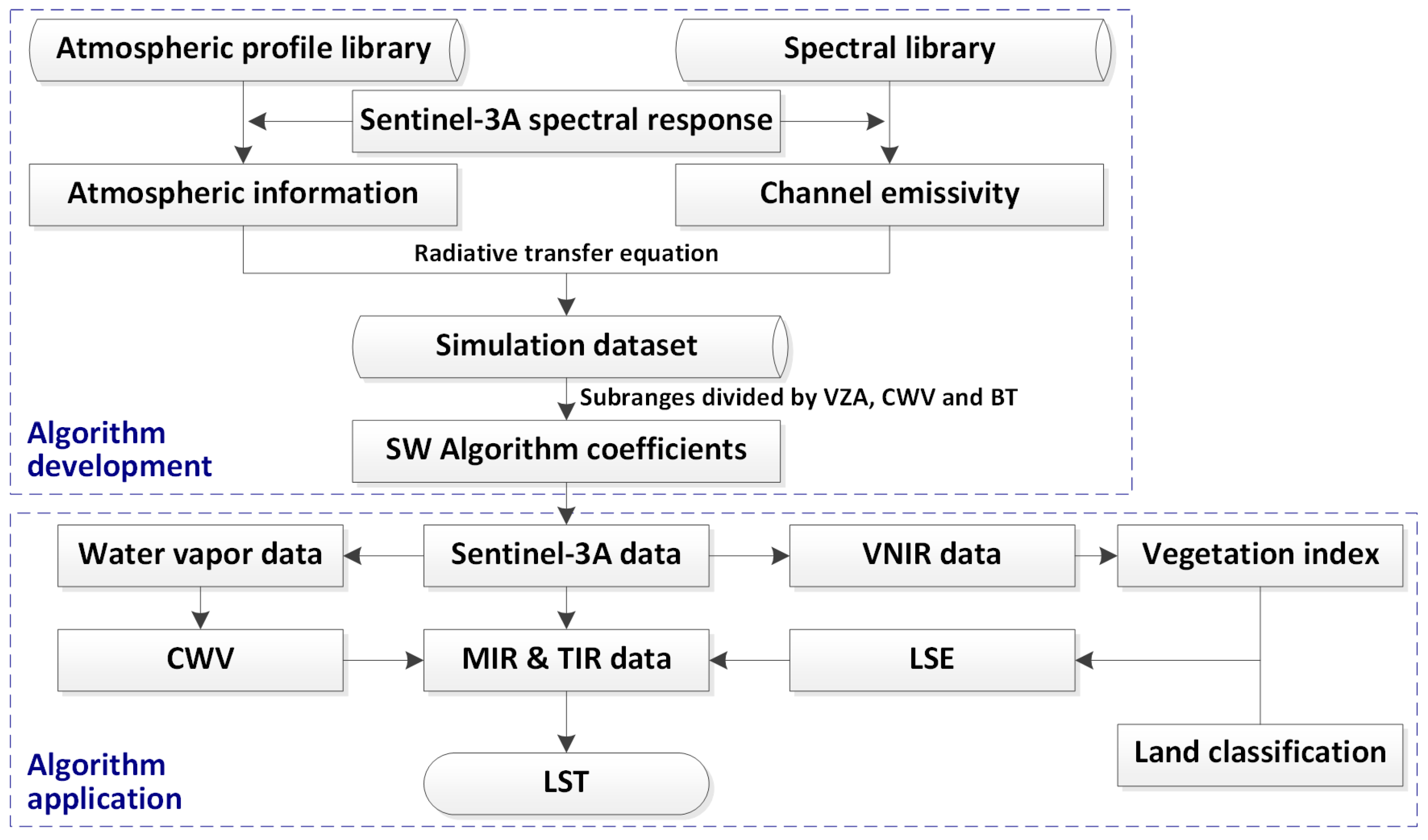
2.2. Algorithm Development

Among the existing retrieval algorithms, the split-window algorithm is an effective and widely used method for several sensors. With the assumption that LSE is known, LST can be retrieved by linear or nonlinear combinations of the brightness temperature at the TOA of two adjacent TIR channels to remove the atmospheric effect. A classical SW algorithm is applied to MODIS [16] and Landsat 8 [7], which can be expressed as follows:

$$LST=a_0+\left(a_1+a_2\frac{1-\epsilon }{\epsilon }+a_3\frac{\Delta \epsilon }{{\epsilon }^2}\right)\frac{T_i+T_j}{2}+\left(a_4+a_5\frac{1-\epsilon }{\epsilon }+a_6\frac{\Delta \epsilon }{{\epsilon }^2}\right)\frac{T_i-T_j}{2}+a_7{\left(T_i-T_j\right)}^2$$

(2)

where a_n (n = 0–7) are algorithm coefficients, which can be determined from the simulated dataset, i and j are two TIR channels centered at about 11 μm and 12 μm, T_i and T_j are the brightness temperatures of the two channels, ε is the average emissivity of the two channels (i.e., ε = (ε_i + ε_j)/2), and Δε is the emissivity difference between the two channels (i.e., Δε = ε_i − ε_j).

Similar to the TIR channel, the MIR channel also contains the information of land surface thermal radiance and can be used for LST retrieval. Moreover, the MIR channel has lower atmospheric attenuation and sensitivity to LSE. Mushkin et al. [17] found that if LSE has an error at 0.02, then it will cause 1 K error for the retrieved results from the TIR channel, but it will only cause 0.5 K error for the retrieved results from the MIR channel. In spite of the advantages of the MIR channel, LST retrieval from MIR data is underdeveloped, because MIR data additionally contain reflected solar irradiance during the daytime, which is nearly equal to and difficult to be separated from the land surface thermal radiance. To avoid the influence of the solar irradiance, the MIR data obtained from the nighttime observation, rather than the daytime observation, is utilized to estimate LST and improve the retrieval accuracy.

As stated above, the SLSTR has one MIR channel (Channel 7) and two TIR channels (Channels 8 and 9), whose spectral responses are shown in Figure 2. Since Channels 8 and 9 are conventional SW channels, the SW algorithm for their daytime data can be developed according to Equation (2). As for the nighttime observation, Channel 7 can be additionally taken into account to make full use of the MIR channel information. Sun and Pinker [18] proposed a new form of SW algorithm that utilizes the difference between the brightness temperatures of MIR and TIR channels, thereby breaking the conventional SW pattern where only the differences between TIR brightness temperatures are used. Inspired by their research and in combination with the algorithm proposed by Wan [16], the current study presents the nighttime algorithm equation as follows:

$$\begin{array}{cc}\hfill LST=b_0+(b_1& +b_2\frac{1-{\epsilon }_{89}}{{\epsilon }_{89}}+b_3\frac{\Delta {\epsilon }_{89}}{{\epsilon }_{89}^2})\frac{T_8+T_9}{2}+\left(b_4+b_5\frac{1-{\epsilon }_{89}}{{\epsilon }_{89}}+b_6\frac{\Delta {\epsilon }_{89}}{{\epsilon }_{89}^2}\right)\frac{T_8-T_9}{2}\hfill \\ & +b_7{\left(T_8-T_9\right)}^2+(b_8\frac{1-{\epsilon }_{78}}{{\epsilon }_{78}}+b_9\frac{\Delta {\epsilon }_{78}}{{\epsilon }_{78}^2})\frac{T_7-T_8}{2}+b_{10}{\left(T_7-T_8\right)}^2\hfill \\ & +b_{11}(\frac{1-{\epsilon }_{79}}{{\epsilon }_{79}}+b_{12}\frac{\Delta {\epsilon }_{79}}{{\epsilon }_{79}^2})\frac{T_7-T_9}{2}+b_{13}{\left(T_7-T_9\right)}^2\hfill \end{array}$$

(3)

where b_n (n = 0–13) are algorithm coefficients obtained from the simulated dataset, T_k (k = 7–9) are the brightness temperatures of channel k, εij is the average emissivity of channels i and j, and Δεij is the emissivity difference between channels i and j.

2.3. Simulation Dataset

To obtain the algorithm coefficients, 946 clear-sky atmospheric profiles of Thermodynamic Initial Guess Retrieval Version 3 (TIGR-3) [19,20], including tropical, mid-latitude, and polar atmospheric information, were selected as input parameters for the atmospheric radiative transfer model MODTRAN (MODerate spectral resolution atmospheric TRANsmittance and radiance code) Version 5.2 to simulate $R_{ai}^{\downarrow }$, $R_{ai}^{\uparrow }$, and τ_i in the three channels of SLSTR [21]. The principle of selection was that one profile was affected by the cloud if any level of relative humidity of the profile was greater than 90%. Among the selected atmospheric profiles, CWVs ranged from 0 to 6.5 g/cm², whereas air temperatures at the bottom layer of the profiles (T₀) ranged from 230 to 310 K [22]. Considering the difference between surface temperature and air temperature during the day and night, LSTs for simulation input were set to nine levels for the daytime algorithm, ranging from T₀ − 10 to T₀ + 30 K, with the step of 5 K, and set to seven levels for the nighttime algorithm, ranging from T₀ − 20 to T₀ + 10 K, with the step of 5 K. That aside, 60 emissivity spectra were selected for simulation from the Advanced Spaceborne Thermal Emission Reflection (ASTER) spectral library version 2 [23] and the University of California–Santa Barbara (UCSB) emissivity library [24], including 10 vegetation, 20 soil, 20 rock, 5 water, and 5 mineral spectra. Moreover, due to the large field of view (about 60°) and ground swath (about 1400 km) of Sentinel-3A images, data simulation was performed under five VZAs, i.e., 0°, 15°, 25°, 35°, and 45°, to reduce the angle effect on LST estimation. Finally, 2,554,200 groups of simulated data were obtained for the daytime algorithm development (946 atmospheric profiles × 9 LSTs × 60 emissivities × 5 VZAs), while 1,986,600 groups of simulated data were obtained for the nighttime algorithm development (946 atmospheric profiles × 7 LSTs × 60 emissivities × 5 VZAs). 70% of the simulated data were selected randomly as a training set to construct the retrieval algorithm, and another 30% of the simulated data were used to test the algorithm. Fully considering different atmosphere, surface, and view conditions, both the training set and the test set could sufficiently represent all the possible combinations.

2.4. Algorithm Coefficients and Analysis

The algorithm coefficients were calculated for each VZA by regression analysis on the basis of the simulation dataset under each condition of VZA. Considering that atmospheric water vapor content had an enormous influence on thermal radiance and caused uncertainty to LST retrieval, the CWVs of the 946 atmospheric profiles were divided into four subranges, in which algorithm coefficients were calculated, respectively. In order to avoid the discontinuity of retrieval results caused by different CWV subranges, an overlap of 0.5 g/cm² was set between two adjacent CWV subranges [7,8,9]. As a consequence, there were 812, 100, 76, and 51 profiles with CWV ranging from 0 to 2.5 g/cm², from 2 to 3.5 g/cm², from 3 to 4.5 g/cm², and from 4 to 6.5 g/cm², respectively.

Moreover, considering that LST might vary tremendously under different conditions, the simulated data were divided into several subranges, according to their temperature under each CWV subrange. Since the true LST was undetermined, brightness temperature (BT) was used for the division. Figure 3 shows the relationship between simulated LST and BT of the two TIR channels (denoted by BT8 and BT9, respectively). The root-mean-square error (RMSE) between simulated LST and BT was denoted by T_diff in Figure 3, from which it was found that BT8 was closer to LST, with a temperature difference of about 2.07 K. Therefore, BT8 was chosen for subrange division. For daytime and nighttime algorithms, BT8 was divided into four subranges, as follows: (0, 285) K, [285, 300) K, [300, 315) K, [315, +∞) K and (0, 280) K, [280, 290) K, [290, 300) K, [300, +∞) K, respectively. As a result, the simulated data were divided into 160 subranges, i.e., 5 VZAs × 4 CWVs × 4 BT8s × 2 times (day and night). For each subrange, the algorithm coefficients of Equations (2) and (3) were calculated by regression analysis separately and stored in a lookup table.

Table 1. Coefficients and root-mean-square errors (RMSEs) of different subranges for the daytime algorithm where view zenith angle (VZA) = 0°.

CWV (g/cm2)	BT (K)	a0	a1	a2	a3	a4	a5	a6	a7	RMSE (K)
										Without Noise	With Noise
[0, 2.5]	(0, 285)	−3.062	1.015	0.167	−0.323	3.559	3.865	15.789	−0.181	0.21	1.32
	[285, 300)	−4.826	1.020	0.192	−0.298	3.402	0.623	−5.283	0.055	0.33	1.43
	[300, 315)	2.899	0.994	0.191	−0.313	2.908	3.614	−13.992	0.144	0.31	1.75
	[315, +∞)	9.103	0.977	0.195	−0.319	2.548	3.524	−12.441	0.123	0.30	1.87
[2, 3.5]	(0, 285)	20.916	0.926	0.174	−0.263	5.756	−0.147	8.598	−0.254	0.43	1.27
	[285, 300)	13.663	0.951	0.187	−0.283	6.372	0.345	−0.756	−0.106	0.53	1.41
	[300, 315)	16.841	0.942	0.199	−0.299	5.041	1.398	−7.915	0.054	0.57	1.71
	[315, +∞)	25.420	0.915	0.214	−0.371	4.985	0.076	−1.549	0.036	0.51	1.93
[3, 4.5]	(0, 285)	47.842	0.829	0.155	−0.189	6.900	3.078	−5.235	−0.352	0.71	1.07
	[285, 300)	13.359	0.949	0.144	−0.178	6.660	6.447	−10.709	−0.042	0.59	1.12
	[300, 315)	9.721	0.964	0.164	−0.194	5.689	3.657	−10.460	0.030	0.81	1.52
	[315, +∞)	63.312	0.796	0.236	−0.256	4.489	−2.393	−9.569	0.084	1.02	1.94
[4, 6.5]	(0, 285)	−10.657	1.033	0.108	−0.117	6.780	−0.212	−8.853	−0.212	0.32	0.58
	[285, 300)	−0.600	0.995	0.121	−0.120	6.558	5.241	−9.541	0.033	0.78	1.07
	[300, 315)	8.622	0.968	0.138	−0.106	5.732	4.703	−14.378	0.053	1.04	1.51
	[315, +∞)	203.901	0.637	−0.332	1.179	−44.482	47.653	−130.253	1.732	1.28	2.08

and

Table 2. Coefficients and RMSEs of different subranges for the nighttime algorithm where VZA = 0°.

CWV (g/cm2)	BT (K)	b0	b1	b2	b3	b4	b5	b6	RMSE (K)
		b7	b8	b9	b10	b11	b12	b13	Without Noise	With Noise
[0, 2.5]	(0, 280)	−3.050	1.015	0.165	−0.281	3.394	−0.032	30.614	0.23	1.19
		−0.366	−6.978	−4.598	0.074	6.010	4.417	−0.091
	[280, 290)	1.036	0.999	0.183	−0.320	4.540	16.407	9.147	0.37	1.49
		−0.139	5.744	−2.027	0.089	−5.493	1.879	−0.078
	[290, 300)	−0.994	1.005	0.190	−0.297	4.420	−21.120	15.620	0.32	1.29
		−0.192	−8.156	2.550	−0.078	7.225	−3.717	0.106
	[300, +∞)	−2.965	1.014	0.196	−0.250	3.117	−30.338	13.061	0.25	1.07
		−0.140	−12.612	3.166	−0.101	11.758	−4.529	0.133
[2, 3.5]	(0, 280)	16.807	0.941	0.160	−0.311	4.809	21.523	−7.853	0.43	1.36
		−0.079	14.058	5.224	0.024	−12.160	−3.424	−0.075
	[280, 290)	15.340	0.947	0.163	−0.283	5.113	23.413	−16.580	0.50	1.37
		0.132	14.299	3.267	0.053	−10.967	−0.761	−0.109
	[290, 300)	10.520	0.962	0.175	−0.266	6.814	−13.047	16.083	0.50	1.14
		−0.409	1.226	7.296	−0.144	1.660	−5.080	0.094
	[300, +∞)	−9.796	1.030	0.203	−0.265	6.798	−38.554	35.950	0.31	0.82
		−0.572	−11.883	5.363	−0.138	13.938	−5.256	0.151
[3, 4.5]	(0, 280)	13.462	0.951	0.082	−0.238	3.172	17.880	−10.185	0.61	1.01
		−0.186	4.671	7.400	−0.076	−8.581	−6.134	−0.063
	[280, 290)	6.348	0.978	0.075	−0.218	5.772	17.963	3.681	0.64	1.11
		−0.195	7.061	10.284	−0.273	−8.638	−7.734	0.104
	[290, 300)	−2.472	1.006	0.121	−0.185	6.454	−2.422	9.853	0.57	0.89
		−0.378	3.098	9.329	−0.247	−0.664	−5.970	0.134
	[300, +∞)	−13.935	1.043	0.183	−0.172	7.051	−25.340	16.953	0.35	0.70
		−0.511	−5.771	5.698	−0.129	8.950	−4.591	0.123
[4, 6.5]	(0, 280)	−40.985	1.140	0.051	−0.156	2.083	11.440	−18.210	0.17	0.46
		−0.096	−7.460	4.087	−0.033	0.024	−4.227	−0.082
	[280, 290)	−31.370	1.110	−0.010	−0.136	5.085	20.570	6.600	0.65	0.88
		−0.363	−3.090	8.271	−0.392	−5.483	−7.983	0.167
	[290, 300)	−14.693	1.047	0.099	−0.121	8.147	−20.388	23.113	0.57	0.58
		−1.045	−6.059	13.139	−0.449	8.040	−9.678	0.302
	[300, +∞)	−32.582	1.102	0.141	−0.102	8.746	−22.234	12.728	0.29	1.00
		−0.708	−6.499	5.360	−0.132	9.772	−4.499	0.132

show the coefficients and the corresponding RMSEs when VZA = 0° for the daytime and nighttime algorithms, respectively. Considering that the retrieval accuracy might be sensitive to the uncertainty of LSE, a random noise of Gaussian distribution with zero mean and 0.01 standard deviation was introduced to LSE, and Equations (2) and (3) with original coefficients were then used to calculate a biased LST. The RMSEs with the random noise in LSE are also listed in Table 1 and Table 2. Figure 4 presents the histograms of LST residual errors (ΔT) for both algorithms. It can be discovered that the absolute value of most residual errors is less than 1 K. For the daytime algorithm, the ratio of $\left|\Delta T\right|$ < 1 K is 96.4%, while that for nighttime is 98.7%. Figure 5 presents the variation of the temperature RMSE (without noise) as the CWV changes under different VZAs. Results suggest that (i) the RMSE shows an increasing trend as the CWV increases, and decreases if the MIR channel is involved in the nighttime algorithm, especially with the case of a large CWV level; (ii) the RMSEs with noise are generally lower than 2 K for the daytime algorithm and 1.5 K for the nighttime algorithm, and the nighttime algorithm is less sensitive to the uncertainty of LSE; and (iii) a larger VZA leads to a larger RMSE. After constructing the algorithm, 30% of the simulated data are used as a test set to evaluate the algorithm. The test results are displayed in Figure 6. The retrieved LST and the simulated LST show a strong correlation with a small error. For the daytime algorithm, the regression determination coefficients are: R² is 0.9996, bias is 0.0033 K, and RMSE is 0.49 K, whereas for the nighttime algorithm, R² is 0.9997, bias is 0.0020 K, and RMSE is 0.38 K. It illustrates that LST can be estimated with the proposed algorithm, and the involvement of the MIR channel can reduce the algorithmic error and improve the retrieval accuracy in theory.

2.5. Acquisition of Algorithm Input Parameters

VZA, BT8, CWV, and LSE are the four vital input parameters for the practical application of the proposed LST retrieval algorithm. Among them, VZA images are provided in the SLSTR Level 1 product at a 10-km scale and can be resampled to a 1-km scale on the basis of the pixel location in the observed image. The BT8 can be directly obtained from surface thermal radiance. The water vapor information is also provided in the SLSTR Level 1 data, which is derived from the European Centre for Medium-Range Weather Forecasts (ECMWF) [15]. Therefore, the estimation of LSE will be introduced in the following discussion.

The classification-based method and the vegetation-index method are two frequently used methods for estimating LSE. Assuming that the same land cover type exhibits very similar emissivity, the classification-based method is a simple but accurate method, as long as the land surface is properly classified, and the emissivity of each class is well known [3,24]. The vegetation-index method is based on the relationship between LSE and the vegetation index, such as the normalized difference vegetation index (NDVI). This method assumes that the surface is only composed of soil and vegetation, and that LSE changes linearly with respect to the vegetation fraction in a pixel [25,26]. This study combines the two above-mentioned methods to obtain a more accurate LSE. Considering the seasonal impact on the classification product, it is assumed that each land class consists of a background component and a vegetation component, according to its feature and structure. The LSE of one pixel changes with a changing vegetation fraction. Thus, the LSE of each pixel can be calculated as follows [27]:

$$\epsilon =c+{\displaystyle \sum }{a}_{\lambda }·{\rho }_{\lambda },\mathrm{NDVI}<{\mathrm{NDVI}}_{\mathrm{s}}\left(\mathrm{barren}\mathrm{soil}\right)$$

(4)

$$\epsilon ={\epsilon }_{v}f+{\epsilon }_s\left(1-f\right)+4\mathrm{d}\epsilon ·f·\left(1-f\right),{\mathrm{NDVI}}_{\mathrm{s}}\le \mathrm{NDVI}\le {\mathrm{NDVI}}_{\mathrm{v}}\left(\mathrm{partly}\mathrm{vegetated}\right)$$

(5)

$$\epsilon ={\epsilon }_v+\mathrm{d}\epsilon ,\mathrm{NDVI}>{\mathrm{NDVI}}_{\mathrm{v}}\left(\mathrm{fully}\mathrm{vegetated}\right)$$

(6)

where a_λ and c are coefficients transferring band reflectance ρ_λ to emissivity [26]. ε_v and ε_s are channel emissivities of the vegetation and background components, respectively, which can be estimated from various emissivity samples in the spectral library. dε is the emissivity increment from the cavity effect, caused by multiple scattering in the pixel [28]. f represents the fractional vegetation cover (FVC), which can be calculated from NDVI [29] as follows:

$$f={\left(\frac{\mathrm{NDVI}-{\mathrm{NDVI}}_{\mathrm{s}}}{{\mathrm{NDVI}}_{\mathrm{v}}-{\mathrm{NDVI}}_{\mathrm{s}}}\right)}^2$$

(7)

where NDVI_v and NDVI_s are the NDVI of fully vegetated pixels and barren soil pixels, usually using the values of 0.86 and 0.2, respectively [30,31]. For the daytime observation, NDVI is calculated from the surface reflectance, which is obtained by applying atmospheric correction to the radiance observed at the TOA. For the nighttime observation, NDVI cannot be calculated from visual and near infrared data since no solar energy in those bands is available. In view of the fact that vegetation remains almost unchanged within a few days, the FVC image of the nighttime observation can be derived from the daytime observation, whose imaging time is close to it.

The MODIS Land Cover Type Product (MCD12Q1) is used in this study. MCD12Q1 is created by supervised classification of MODIS reflectance data [32,33]. It provides global maps of land cover with 500-m spatial resolution at annual time steps for six different land cover legends, including the International Geosphere–Biosphere Programme (IGBP) land cover classification [34,35], the University of Maryland (UMD) classification scheme [36], the Biome classification scheme [37], the LAI/fPAR Biome scheme [38], the Plant Functional Type scheme [39], and a new three-layer legend based on the Land Cover Classification System (LCCS) from the Food and Agriculture Organization [40,41]. The first land cover legend of MCD12Q1 (i.e., IGBP) is used to obtain the LSE for the proposed algorithm, and it contains 17 land cover types globally. To obtain the component emissivity of each land cover type in the MIR and TIR bands, some emissivity samples of various land surfaces are selected from the spectral library [27]. Different land cover types and the estimated emissivities of the three bands are listed in

Table 3. Component emissivities of different land cover types in the MIR and TIR bands.

Land Cover Types	εv			εs
	Ch-7	Ch-8	Ch-9	Ch-7	Ch-8	Ch-9
Evergreen Needleleaf Forests	0.981	0.983	0.982	0.855	0.970	0.975
Evergreen Broadleaf Forests	0.984	0.983	0.982	0.855	0.970	0.975
Deciduous Needleleaf Forests	0.981	0.983	0.982	0.855	0.970	0.975
Deciduous Broadleaf Forests	0.984	0.983	0.982	0.855	0.970	0.975
Mixed Forests	0.983	0.983	0.982	0.855	0.970	0.975
Closed Shrublands	0.983	0.982	0.983	0.776	0.971	0.974
Open Shrublands	0.983	0.982	0.983	0.776	0.971	0.974
Woody Savannas	0.984	0.983	0.983	0.816	0.971	0.975
Savannas	0.984	0.982	0.984	0.776	0.971	0.974
Grasslands	0.984	0.982	0.984	0.776	0.971	0.974
Permanent Wetlands	0.984	0.982	0.984	0.897	0.983	0.982
Croplands	0.984	0.982	0.984	0.827	0.974	0.978
Urban and Build-up	-	-	-	0.931	0.959	0.966
Cropland–Natural Vegetation Mosaics	0.984	0.982	0.984	0.827	0.974	0.978
Snow and Ice	-	-	-	0.979	0.990	0.974
Barren or Sparsely Vegetated	0.941	0.954	0.953	0.848	0.968	0.975
Water Bodies	-	-	-	0.973	0.991	0.986

.

3. Application and Validation

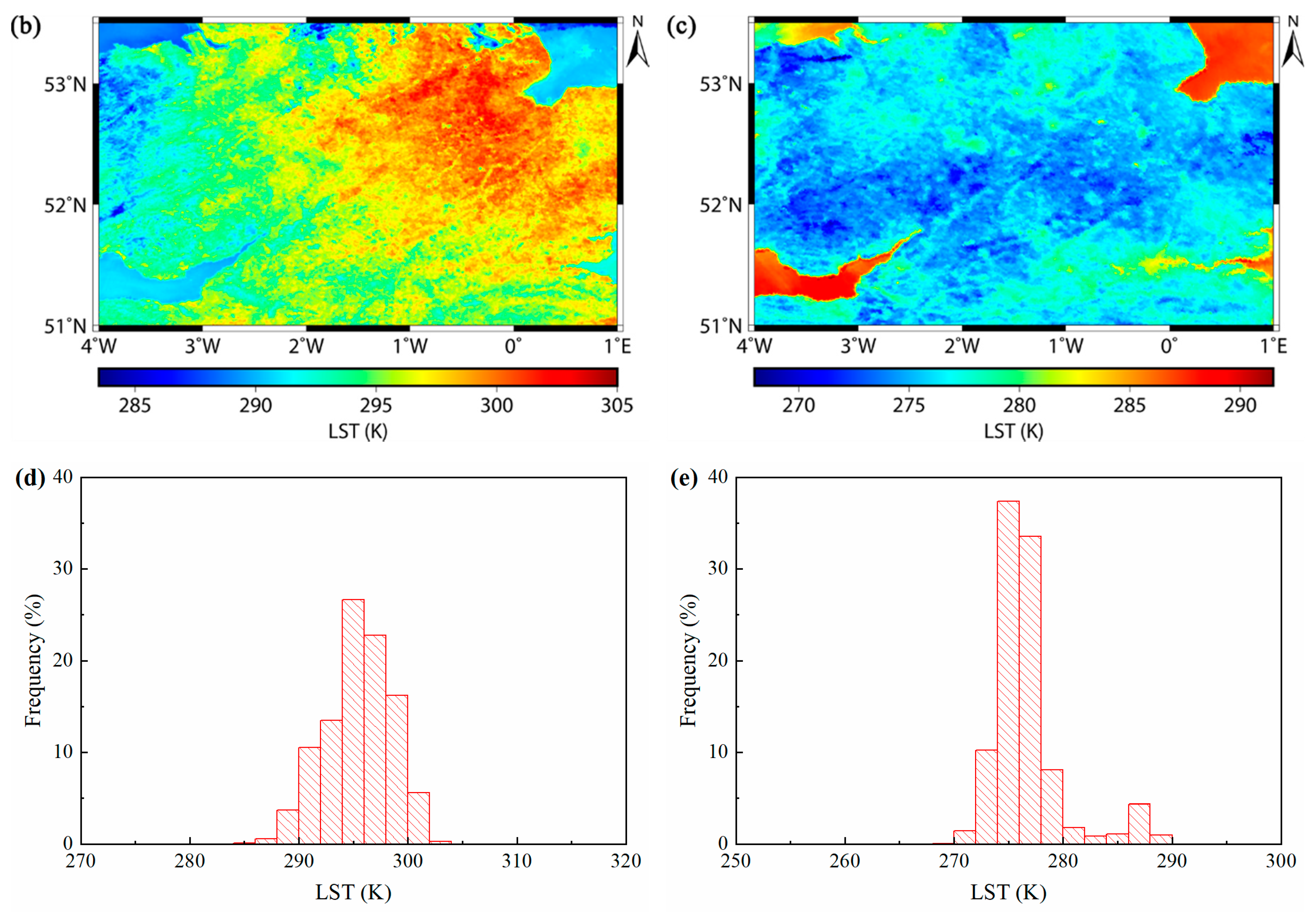
3.1. Application in LST Retrieval

The proposed algorithm is applied when retrieving the LSTs of two study areas for both daytime and nighttime observations as examples. The first study area is located in the north of China (denoted by Region 1), as shown in Figure 7a. The land of this region mostly contained forest (dark red) in the middle part, cropland (red) in the southeast part, grassland (light red) in the northwest part, urban areas (gray), and water surface (dark). The daytime and nighttime images were acquired on 24 and 23 September 2018, respectively. The LST retrieval results of the daytime and nighttime observations are shown in Figure 7b,c, respectively. Figure 7d,e shows the corresponding LST histograms. The second study area is located in the south of the UK (denoted by Region 2; see Figure 8a) and is mainly covered by forest, cropland, grassland, ocean surface, and built-up area. The daytime and nighttime images were acquired on 27 and 28 September 2018, respectively. The LST retrieval results of the daytime and nighttime observations are shown in Figure 8b,c, respectively, and the corresponding LST histograms are presented in Figure 8d,e. In Region 1, the LST of daytime and nighttime observations ranged from 280 to 310 K and 270 to 300 K, respectively. In the daytime image (Figure 7b), the LST of urban pixels was higher than that of the cropland, grassland, and water surface, but in the nighttime image, the LST of water surface got the largest value, because the water had heat capacity, and its cooling rate was consequently lower than that of other land covers. The urban surface still had larger LST in the nighttime image, due to the heat island effect. In Region 2, the urban surface similarly presented larger LST in the daytime than the nonurban areas and ocean surface, whereas the ocean surface had a higher temperature than the land surface in the nighttime. Note that although the split-window algorithm was primarily proposed to retrieve land surface temperature, it is also applied to estimating the surface temperature of the coastal ocean. In this case, the ocean surface atmosphere was assumed to have no remarkable difference to the land surface, and the pixel emissivity was regarded as that of a water body in Table 3.

3.2. Validation Using Ground-Based Measurement

To validate the retrieval result and evaluate the algorithm accuracy, the surface temperature is calculated from the ground flux measurement of several observation sites and regarded as the reference value of LST to make the comparison. Four Surface Radiation Budget Network (SURFRAD) sites in the USA [42] and three Peking University Land Surface Temperature Network (PKULSTNet) sites in China, whose detailed information is listed in

Table 4. Detailed information and validation results of each ground site.

Site Names	Project	Latitude	Longitude	Land Cover	Bias (K) Day/Night	RMSE (K) Day/Night
Bondville_IL (BND)	SURFRAD	40.05°N	88.37°W	Cropland	1.18/0.36	2.99/1.02
Goodwin_Creek_MS (GCM)	SURFRAD	34.25°N	89.87°W	Pasture	0.03/1.92	1.60/2.51
Penn_State_PA (PSU)	SURFRAD	40.72°N	77.93°W	Cropland	1.03/1.79	2.15/2.88
Sioux_Falls_SD (SXF)	SURFRAD	43.73°N	96.62°W	Cropland	0.96/0.77	1.62/1.27
Hebei_Chengde (HBC)	PKULSTNet	42.41°N	117.25°E	Grassland	−0.96/0.56	1.47/1.68
Henan_Hebi (HNH)	PKULSTNet	35.72°N	114.32°E	Cropland	−0.10/0.73	2.41/1.60
InnerMongolia_Baotou (IMB)	PKULSTNet	41.35°N	111.21°E	Grassland	1.81/−0.11	2.52/1.42

, are used to validate the result. The land cover types of the seven sites are cropland or grassland, which is relatively homogeneous and is beneficial for validating the retrieved LST.

For the SURFRAD sites, the LST can be calculated from longwave radiation measurement at an uncertainty of 0.2–0.5 K, given that the error of broadband emissivity is about ±0.02. Moreover, the pyrgeometer measurement error is about 3–5 W/m², equivalent to an error of 0.5–0.8 K in temperature. Therefore, the total ground LST error can be estimated as $e=\sqrt{e_1^2+e_2^2}$, which ranges from 0.53 to 0.94 K. The sites collect surface upward thermal infrared irradiance $L^{\uparrow }$ and atmospheric downward thermal infrared irradiance $R^{\downarrow }$ at the wavelength range of 3–50 μm per minute [42]. On the basis of the thermal radiative transfer equation of the near surface (in Equation (1), ${\tau }_i$ = 1 and $R_{ai}^{\uparrow }$ = 0) and the Stefan–Boltzmann law, the ground-measured reference surface temperature can be calculated as follows:

$$T_{\mathrm{ground}}={\left[\frac{L^{\uparrow }-\left(1-\overline{\epsilon }\right)R^{\downarrow }}{\overline{\epsilon }\sigma }\right]}^{\frac{1}{4}}$$

(8)

where σ is the Stefan–Boltzmann constant with a value of 5.67 × 10⁻⁸ W·m⁻²·K⁻⁴, and $\overline{\epsilon }$ is the ground broadband emissivity (BBE). We applied the technique in Equations (4)–(6) to estimate the BBE for the ground measurement, but unlike the pixel emissivity, the broadband (8–13.5 μm) component emissivity was used (rather than the channel component emissivity) for BBE calculation, which proved to be the best for estimating the net longwave radiation under clear-sky conditions. [27,43]. The NDVI and FVC for the ground observation are obtained from the corresponding satellite data.

For the PKULSTNet sites, the radiometer measurement error is 0.113 K, according to the instrument document. With the addition of the uncertainty of broadband emissivity, as mentioned above (0.2–0.5 K), the total ground LST error is about 0.23–0.51 K, in theory. The radiometers of PKULSTNet are sensitive to the wavelength, ranging from 8 to 14 μm, but unlike the SURFRAD sites, the measurement outputs of the PKULSTNet sites are the ground-leaving brightness temperature T₁ and the atmosphere brightness temperature T₂, rather than upward and downward irradiance. The integral of the Planck’s law over the wavelength from 8 to 14 μm can be defined as

$$M={\sigma }^{\prime }{T}^4$$

(9)

where M is the total irradiance over 8–14 μm, σ′ is a constant, which is not equal to the Stefan–Boltzmann constant, and T is temperature. Thus, T_ground can be calculated as

$$T_{\mathrm{ground}}={\left[\frac{{\sigma }^{\prime }{T}_1^4-\left(1-\overline{\epsilon }\right){\sigma }^{\prime }{T}_2^4}{\overline{\epsilon }{\sigma }^{\prime }}\right]}^{\frac{1}{4}}={\left[\frac{T_1^4-\left(1-\overline{\epsilon }\right)T_2^4}{\overline{\epsilon }}\right]}^{\frac{1}{4}}$$

(10)

Because the result of Equation (10) is independent of the value of σ′, we think that the calculation of T_ground will not be strongly influenced by using a spectral wavelength from 8 to 14 μm.

Over the seven sites, a total of 327 clear-sky SLSTR images were collected in 2017 and 2018, including 148 daytime images and 179 nighttime images, and their LSTs were then retrieved using the above proposed daytime and nighttime split-window algorithms, respectively. Meanwhile, in order to make a direct comparison, the corresponding ground-measured LST was calculated from Equations (8) and (10). Because the time of ground and satellite measurement cannot match exactly, the average of the 10-min ground-measured temperature before and after satellite overpassing was used as the reference surface temperature. Figure 9 displays the scatter diagrams between satellite-retrieved LST (denoted by LST_retrieval) and ground temperature (denoted by LST_ground) in both daytime and nighttime observations. Most points were along the 1:1 line. For the daytime and nighttime algorithm, the temperature bias was 0.62 K and 0.79 K and the RMSE was 2.24 K and 1.77 K, respectively. The above-mentioned results indicated that the nighttime algorithm showed higher retrieval accuracy (about 0.5 K) than the daytime algorithm. However, the temperature bias, larger than 0 for both daytime and nighttime, meant that the LST from the satellite was slightly overestimated, especially for high temperature in the nighttime.

Table 4 also lists the temperature bias and RMSE of each site. Three sites BND, SXF, and IMB had a relatively smaller temperature error in the nighttime, whereas the sites GCM and PSU had an RMSE larger than 2.0 K. Meanwhile, in the daytime, the sites GCM, SXF, and HBC had a temperature error lower than 2.0 K, and the rest had an error larger than 2.0 K, with the BND site having the largest error of about 3.0 K. The bias of each site was not as high as the RMSE. Five sites in seven had a bias less than 1.0 K, even with some near 0. According to the present validation results, the temperature error from the proposed split-window algorithms probably ranged from 1.5 to 2.5 K. However, the temperature error may be caused by the uncertainty of the split-window algorithm itself and the input parameters (water vapor and emissivity), and may also be affected by the surface inhomogeneity in the SLSTR 1-km pixel scale that resulted in the ground-point measurement not being able to stand for the pixel ground LST.

4. Discussions and Conclusions

The current study proposed a modified SW algorithm to retrieve LST from Sentinel-3A SLSTR MIR and TIR data to make full use of the spectral information and improve the retrieval accuracy. For the daytime observation, only TIR data (Channels 8 and 9) were used to develop the algorithm, similar to the conventional SW algorithm. On the other hand, for the nighttime observation, the MIR data (Channel 7), with a higher atmospheric transmittance and a lower sensitivity to land surface emissivity, was also considered to establish a new equation of the three-channel SW algorithm. To develop the new algorithm, atmospheric radiative transfer model MODTRAN was applied to generate quantities of simulated data, from which the algorithm coefficients were obtained by regression analysis. In order to improve the accuracy of the algorithm, the dataset was then divided into several subranges, according to viewing zenith angle, atmospheric water vapor, and observed brightness temperature, and consequently, the algorithm coefficients were calculated in each subrange separately. Simulation results showed that the proposed algorithm could estimate LST with accuracy better than 1 K on average.

The algorithms were applied to real images of northern China and southern UK, and the retrieval LST captured the surface features for both daytime and nighttime. For validation and evaluation, a total of 327 clear-sky Sentinel-3A SLSTR images, including 148 daytime and 179 nighttime images, were collected, and their retrieved LST was compared with ground-measured LSTs over seven sites. Results show that for the daytime algorithm, the bias of LST was 0.62 K and the RMSE of LST was 2.24 K, whereas for the nighttime algorithm, the bias and RMSE were 0.79 K and 1.77 K, respectively. Results showed that LST could be estimated with an error mostly within 1.5 K to 2.5 K, using the proposed algorithm, and the nighttime algorithm involved with MIR data had a lower error (about 0.5 K) than the daytime algorithm.

More investigations are expected to improve the LST retrieval accuracy. Future work will focus on investigating the influence of the atmosphere and the additional channel. First, as mentioned above, in the algorithm development, there were 812 atmospheric profiles whose CWV was less than 2.5 g/cm² among all of the 946 profiles. Therefore, dry atmospheric profiles took the major part in the simulation dataset, and the algorithm was established mainly based on dry atmosphere. The retrieval accuracy may decrease when the water vapor content is high. To minimize this effect, more representative profiles should be applied to optimize the current algorithm in future work. Moreover, since it is difficult to obtain the aerosol loading from SLSTR observation, especially for the nighttime, the current paper only used a default rural aerosol model (with a visibility of 23 km) in the simulation dataset for algorithm development. Although the error caused by the aerosol is slight compared with water vapor, it still has an impact on LST retrieval accuracy [44]. Therefore, further investigation will concern the impact of the aerosol or thin cloud on the retrieval result. Moreover, some local split-window algorithms that only use atmospheric profiles and surface emissivity over a specified area are promising for retrieval improvement. Although more channels can provide additional spectral information and the MIR channel has its unique advantages, the error introduced by using more channels should also be emphasized. More channels may bring additional errors, like observation, radiometric calibration, and LSE estimation error. Although the nighttime algorithm shows a better performance than the daytime algorithm, it remains necessary to find out how the additional channel influences the retrieval result, as it is the basis to further improve the algorithm.

References

1. Li, Z.-L.; Becker, F. Feasibility of land surface temperature and emissivity determination from AVHRR data. Remote Sens. Environ. 1993, 43, 67–85. [Google Scholar] [CrossRef]
2. Valor, E.; Caselles, V. Mapping land surface emissivity from NDVI: Application to European, African, and south American areas. Remote Sens. Environ. 1996, 57, 167–184. [Google Scholar] [CrossRef]
3. Li, Z.-L.; Tang, B.-H.; Wu, H.; Ren, H.; Yan, G.; Wan, Z.; Trigo, I.F.; Sobrino, J.A. Satellite-derived land surface temperature: Current status and perspectives. Remote Sens. Environ. 2013, 131, 14–37. [Google Scholar] [CrossRef]
4. Mcmillin, L.M. Estimation of sea surface temperatures from two infrared window measurements with different absorption. J. Geophys. Res. 1975, 80, 5113–5117. [Google Scholar] [CrossRef]
5. Ren, H.; Liu, R.; Yan, G.; Mu, X.; Li, Z.-L.; Nerry, F.; Liu, Q. Angular normalization of land surface temperature and emissivity using multiangular middle and thermal infrared data. IEEE Trans. Geosci. Remote Sens. 2014, 52, 4913–4931. [Google Scholar] [CrossRef]
6. Wan, Z.; Dozier, J. A generalized split-window algorithm for retrieving land-surface temperature from space. IEEE Trans. Geosci. Remote Sens. 1996, 34, 892–905. [Google Scholar] [CrossRef]
7. Du, C.; Ren, H.; Qin, Q.; Meng, J.; Zhao, S. A practical split-window algorithm for estimating land surface temperature from Landsat 8 data. Remote Sens. 2015, 7, 647–665. [Google Scholar] [CrossRef]
8. Tang, B.-H.; Bi, Y.; Li, Z.-L.; Xia, J. Generalized split-window algorithm for estimate of land surface temperature from Chinese geostationary FengYun meteorological satellite (FY-2C) data. Sensors 2008, 8, 933–951. [Google Scholar] [CrossRef]
9. Ye, X.; Ren, H.; Liu, R.; Qin, Q.; Liu, Y.; Dong, J. Land surface temperature estimate from Chinese gaofen-5 satellite data using split-window algorithm. IEEE Trans. Geosci. Remote Sens. 2017, 55, 5877–5888. [Google Scholar] [CrossRef]
10. Sun, D.; Pinker, R.T. Estimation of land surface temperature from a geostationary operational environmental satellite (GOES-8). J. Geophys. Res. Atmos. 2003, 108, 4326. [Google Scholar] [CrossRef]
11. Zhao, E.; Qian, Y.; Wang, N.; Ma, L.; Tang, L. Retrieval of night-time land surface temperature from two mid-infrared channels data. J. Infrared Millim. Waves 2014, 33, 303–310. [Google Scholar] [CrossRef]
12. Zhao, E.; Qian, Y.; Gao, C.; Huo, H.; Jiang, X.; Kong, X. Land surface temperature retrieval using airborne hyperspectral scanner daytime mid-infrared data. Remote Sens. 2014, 6, 12667–12685. [Google Scholar] [CrossRef]
13. Donlon, C.; Berruti, B.; Buongiorno, A.; Ferreira, M.-H.; Féménias, P.; Frerick, J.; Goryl, P.; Klein, U.; Laur, H.; Mavrocordatos, C.; et al. The global monitoring for environment and security (GMES) Sentinel-3 mission. Remote Sens. Environ. 2012, 120, 37–57. [Google Scholar] [CrossRef]
14. Ghent, D.J.; Corlett, G.K.; Göttsche, F.-M.; Remedios, J.J. Global land surface temperature from the along-track scanning radiometers. J. Geophys. Res. Atmos. 2017, 122, 12167–12193. [Google Scholar] [CrossRef]
15. Ruescas, A.B.; Jiménez-Muñoz, J.C.; Sobrino, J.A. SEN4LST DEV5: LST Retrieval—Algorithm Theoretical Basis Document (ATBD); Technical Report; The European Space Research and Technology Centre: Frascati, Italy, 2012. [Google Scholar] [CrossRef]
16. Wan, Z. New refinements and validation of the collection-6 MODIS land-surface temperature/emissivity product. Remote Sens. Environ. 2014, 140, 36–45. [Google Scholar] [CrossRef]
17. Mushkin, A.; Balick, L.K.; Gillespie, A.R. Extending surface temperature and emissivity retrieval to the mid-infrared (3–5 μm) using the multispectral thermal imager (MTI). Remote Sens. Environ. 2005, 98, 141–151. [Google Scholar] [CrossRef]
18. Sun, D.; Pinker, R.T. Retrieval of surface temperature from the MSG-SEVIRI observations: Part I. methodology. Int. J. Remote Sens. 2007, 28, 5255–5272. [Google Scholar] [CrossRef]
19. Chédin, A.; Scott, N.A.; Wahiche, C.; Moulinier, P. The improved initialization inversion method: A high resolution physical method for temperature retrievals from satellites of the TIROS-N series. J. Appl. Meteorol. 1985, 24, 128–143. [Google Scholar] [CrossRef]
20. Chevallier, F.; Chéruy, F.; Scott, N.A.; Chédin, A. A neural network approach for a fast and accurate computation of a longwave radiative budget. J. Appl. Meteorol. 1998, 37, 1385–1397. [Google Scholar] [CrossRef]
21. Berk, A.; Anderson, G.P.; Acharya, P.K.; Bernstein, L.S.; Muratov, L.; Lee, J.; Fox, M.; Adler-Golden, S.M.; Chetwynd, J.H.; Hoke, M.L.; et al. Modtran5: A reformulated atmospheric band model with auxiliary species and practical multiple scattering options. Multispectral Hyperspectral Remote Sens. Instrum. Appl. II 2005, 5655, 88–95. [Google Scholar] [CrossRef]
22. Ren, H.; Du, C.; Liu, R.; Qin, Q.; Yan, G.; Li, Z.-L.; Meng, J. Atmospheric water vapor retrieval from Landsat 8 thermal infrared images. J. Geophys. Res. Atmos. 2015, 120, 1723–1738. [Google Scholar] [CrossRef]
23. Baldridge, A.M.; Hook, S.J.; Grove, C.I.; Rivera, G. The ASTER spectral library version 2.0. Remote Sens. Environ. 2009, 113, 711–715. [Google Scholar] [CrossRef]
24. Snyder, W.C.; Wan, Z.; Zhang, Y.; Feng, Y.-Z. Classification-based emissivity for land surface temperature measurement from space. Int. J. Remote Sens. 1998, 19, 2753–2774. [Google Scholar] [CrossRef]
25. Sobrino, J.A.; Raissouni, N. Toward remote sensing methods for land cover dynamic monitoring: Application to morocco. Int. J. Remote Sens. 2000, 21, 353–366. [Google Scholar] [CrossRef]
26. Tang, B.-H.; Shao, K.; Li, Z.-L.; Wu, H.; Tang, R. An improved NDVI-based threshold method for estimating land surface emissivity using MODIS satellite data. Int. J. Remote Sens. 2015, 36, 4864–4878. [Google Scholar] [CrossRef]
27. Ren, H.; Liu, R.; Qin, Q.; Fan, W.; Yu, L.; Du, C. Mapping finer-resolution land surface emissivity using Landsat images in China. J. Geophys. Res. Atmos. 2017, 122, 6764–6781. [Google Scholar] [CrossRef]
28. Caselles, E.; Valor, E.; Abad, F.; Caselles, V. Automatic classification-based generation of thermal infrared land surface emissivity maps using AATSR data over Europe. Remote Sens. Environ. 2012, 124, 321–333. [Google Scholar] [CrossRef]
29. Carlson, T.N.; Ripley, D.A. On the relation between NDVI, fractional vegetation cover, and leaf area index. Remote Sens. Environ. 1997, 62, 241–252. [Google Scholar] [CrossRef]
30. Prihodko, L.; Goward, S.N. Estimation of air temperature from remotely sensed surface observations. Remote Sens. Environ. 1992, 60, 335–346. [Google Scholar] [CrossRef]
31. Tang, R.; Li, Z.-L.; Tang, B.-H. An application of the Ts-VI triangle method with enhanced edges determination for evapotranspiration estimation from MODIS data in arid and semi-arid regions: Implementation and validation. Remote Sens. Environ. 2010, 114, 540–551. [Google Scholar] [CrossRef]
32. Friedl, M.A.; Mciver, D.K.; Hodges, J.C.F.; Zhang, X.Y.; Muchoney, D.; Strahler, A.H.; Woodcock, C.E.; Gopal, S.; Schneider, A.; Cooper, A.; et al. Global land cover mapping from modis: Algorithms and early results. Remote Sens. Environ. 2002, 83, 287–302. [Google Scholar] [CrossRef]
33. Friedl, M.A.; Sulla-Menashe, D.; Tan, B.; Schneider, A.; Ramankutty, N.; Sibley, A.; Huang, X. Modis collection 5 global land cover: Algorithm refinements and characterization of new datasets. Remote Sens. Environ. 2010, 114, 168–182. [Google Scholar] [CrossRef]
34. Loveland, T.R.; Belward, A.S. The international geosphere biosphere programme data and information system global land cover data set (DISCover). Acta Astronaut. 1997, 41, 681–689. [Google Scholar] [CrossRef]
35. Belward, A.S.; Estes, J.E.; Kline, K.D. The IGBP-DIS global 1-km land-cover data set discover: A project overview. Photogramm. Eng. Remote Sens. 1999, 65, 1013–1020. [Google Scholar]
36. Hansen, M.C.; Defries, R.S.; Townshend, J.R.; Sohlberg, R. Global land cover classification at 1 km spatial resolution using a classification tree approach. Int. J. Remote Sens. 2000, 21, 1331–1364. [Google Scholar] [CrossRef]
37. Running, S.W.; Nemani, R.R.; Heinsch, F.A.; Zhao, M.; Reeves, M.C.; Hashimoto, H. A continuous satellite-derived measure of global terrestrial primary production. BioScience 2004, 54, 547. [Google Scholar] [CrossRef]
38. Myneni, R.B.; Hoffman, S.; Knyazikhin, Y.; Privette, J.L.; Glassy, J.; Tian, Y.; Wang, Y.; Song, X.; Zhang, Y.; Smith, G.R.; et al. Global products of vegetation leaf area and fraction absorbed PAR from year one of MODIS data. Remote Sens. Environ. 2002, 83, 214–231. [Google Scholar] [CrossRef]
39. Bonan, G.B. Landscapes as patches of plant functional types: An integrating concept for climate and ecosystem models. Glob. Biogeochem. Cycles 2002, 16, 1021. [Google Scholar] [CrossRef]
40. Di Gregorio, A. Land Cover Classification System: Classification Concepts and User Manual: LCCS; Number 8; Food and Agriculture Organization: Rome, Italy, 2005. [Google Scholar]
41. Sulla-Menashe, D.; Friedl, M.A.; Krankina, O.N.; Baccini, A.; Woodcock, C.E.; Sibley, A.; Sun, G.; Kharuk, V.; Elsakov, V. Hierarchical mapping of Northern Eurasian land cover using MODIS data. Remote Sens. Environ. 2011, 115, 392–403. [Google Scholar] [CrossRef]
42. Wang, K.; Liang, S. Evaluation of ASTER and MODIS land surface temperature and emissivity products using long-term surface longwave radiation observations at SURFRAD sites. Remote Sens. Environ. 2009, 113, 1556–1565. [Google Scholar] [CrossRef]
43. Ogawa, K.; Schmugge, T. Mapping surface broadband emissivity of the Sahara desert using ASTER and MODIS data. Earth Interact. 2004, 8, 1–14. [Google Scholar] [CrossRef]
44. Fan, X.; Tang, B.-H.; Wu, H.; Yan, G.; Li, Z.-L.; Zhou, G.; Shao, K.; Bi, Y. Extension of the generalized split-window algorithm for land surface temperature retrieval to atmospheres with heavy dust aerosol loading. IEEE J. Sel. Top. Appl. Earth Obs. Remote Sens. 2015, 8, 825–834. [Google Scholar] [CrossRef]
Figure 1. Technique process of the proposed algorithm.
Remotesensing 11 00650 g001
Figure 2. Spectral response filters of the middle infrared (MIR) and thermal infrared (TIR) channels of Sentinel-3A Sea and Land Surface Temperature Radiometer (SLSTR).
Remotesensing 11 00650 g002
Figure 3. Relationship between simulated land surface temperature (LST) and brightness temperature (BT) of the two TIR channels.
Remotesensing 11 00650 g003
Figure 4. Histograms of LST residual errors for (a) daytime algorithm and (b) nighttime algorithm.
Remotesensing 11 00650 g004
Figure 5. Variation of the temperature RMSE (without noise) as the column water vapor (CWV) changes under different VZAs for (a) daytime algorithm and (b) nighttime algorithm.
Remotesensing 11 00650 g005
Figure 6. Algorithm test results for (a) daytime algorithm and (b) nighttime algorithm.
Remotesensing 11 00650 g006
Figure 7. Application in Region 1. (a) Location and false-color image; (b) daytime LST result; (c) nighttime LST result; (d) daytime LST histogram; (e) nighttime LST histogram.
Remotesensing 11 00650 g007
Figure 8. Application in Region 2. (a) Location and false-color image; (b) daytime LST result; (c) nighttime LST result; (d) daytime LST histogram; (e) nighttime LST histogram.
Remotesensing 11 00650 g008aRemotesensing 11 00650 g008b
Figure 9. Ground validation in different sites for (a) daytime algorithm and (b) nighttime algorithm.
Remotesensing 11 00650 g009