Enhanced Back-Projection as Postprocessing for Pansharpening

1
School of Mathematics and Statistics, Xi’an Jiaotong University, Xi’an 710049, China
2
School of Mathematics and Computer Application, Shangluo University, Shangluo 726000, China
*
Author to whom correspondence should be addressed.
Remote Sens. 2019, 11(6), 712; https://0-doi-org.brum.beds.ac.uk/10.3390/rs11060712
Submission received: 22 February 2019
/
Revised: 21 March 2019
/
Accepted: 21 March 2019
/
Published: 25 March 2019
(This article belongs to the Special Issue Advances in Remote Sensing Image Fusion)
Abstract
:Pansharpening is the process of integrating a high spatial resolution panchromatic image with a low spatial resolution multispectral image to obtain a multispectral image with high spatial and spectral resolution. Over the last decade, several algorithms have been developed for pansharpening. In this paper, a technique, called enhanced back-projection (EBP), is introduced and applied as postprocessing on the pansharpening. The proposed EBP first enhances the spatial details of the pansharpening results by histogram matching and high-pass modulation, followed by a back-projection process, which takes into account the modulation transfer function (MTF) of the satellite sensor such that the pansharpening results obey the consistency property. The EBP is validated on four datasets acquired by different satellites and several commonly used pansharpening methods. The pansharpening results achieve substantial improvements by this postprocessing technique, which is widely applicable and requires no modification of existing pansharpening methods.
1. Introduction
Due to physical and technical constraints [1], current optical earth observation satellites such as QuickBird, IKONOS, GeoEye-1, and WorldView-2, instead of providing images with both high spatial and spectral resolutions, can only produce a high spatial resolution panchromatic (PAN) image and a low spatial resolution multispectral (MS) image over the same area. The spatial and spectral resolutions allow identifying structures in the images through the electromagnetic spectrum and geometrical information, and thus are very important to many remote sensing tasks, such as change detection [2], digital soil mapping [3], and visual image analysis [4]. In order to benefit from these two kinds of information, the PAN and MS images can be integrated to get a MS image with both high spatial and spectral resolutions. This integrating process is classically referred to as pansharpening, which can be viewed as a special kind of image fusion [5] or super-resolution, Loncan15.
In the last two decades, many methods have been developed in the literature of pansharpening. They can be divided into two main groups: component substitution (CS) and multiresolution analysis (MRA) [6]. The CS group is usually called spectral class as the details that shall be injected into the upsampled MS bands are extracted from the PAN image by means of a spectral transformation of MS pixels, whereas the MRA group is also named spatial class as the injected details are extracted with respect to a spatial transformation of the PAN image, mostly relying on linear shift-invariant digital filters [7]. Classic methods of the CS or spectral family include the generalized Intensity-Hue-Saturation (GIHS) [8], the principal component analysis (PCA) [9], the Gram–Schmidt (GS) decomposition [10] and its adaptive version (GSA) [11], the partial replacement adaptive component substitution (PRACS) [12], the band-dependent spatial-detail (BDSD) [13], among many others [14,15,16]. Although these methods are easy to implement and can acquire outstanding spatial details, they may suffer from spectral distortion. On the contrary, the MRA or spatial class usually achieves a better spectral quality in the pansharpening result than that of the CS class. The representative methods belonging to the MRA class are high-pass modulation (HPM) [17], which is also named smoothing filter-based intensity modulation (SFIM) [18], generalized Laplacian pyramid (GLP) [19], morphological-based fusion (MF) [20], among many others [21,22]. However, the MRA methods may make the fused results produce ring artifacts, leading to spatial distortion.
There is in fact a tradeoff between the classes of CS and MRA methods in the improvement of spatial quality and the maintain of spectral information. In order to take advantage of the complimentary performances of the two classes, researchers have explored the hybrid methods of the two classes. For example, Núñez et al. [23] have proposed the additive wavelet luminance proportional (AWLP) method by combining the “à trous” wavelet transform with the GIHS method. Liao et al. [24] have proposed the guided filter PCA (GFPCA) method, which applies a guided filter in the PCA domain. Shah et al. [25] have proposed a combined adaptive PCA algorithm based on the discrete contourlet transform. In addition, the performances of the CS and/or MRA methods can also be improved by considering the modulation transfer function (MTF) (The MTF is a function of spatial resolution, and in theory the MTF decreases as the spatial resolution increase [26].) of the instruments [19] or by the elaborate design of injection gains in a context-adaptive manner [27].
In general, the restoration of ideal high resolution MS image from its degraded version is an ill-posed inverse problem. Different from the CS, MRA and hybrid classes, many regularization- and/or optimization-based methods have been proposed to resolve this ill-posed inverse problem [28], such as the total variation [29,30] or sparse regularization [31,32,33,34,35,36]. These methods usually achieve a better pansharpening quality, however, the high computational complexity makes them unsuitable for practical applications. There are still some works which rely on Bayesian framework [37] to solve this problem. Very recently, deep learning methods have been introduced into remote sensing problems [38,39], and several methods have been proposed to address pansharpening [40,41,42]. However, their performances would degrade if there are not enough training images. Detailed surveys of pansharpening methods can be found in [6]. Moreover, pansharpening methods have been recently expanded to sharp the hyperspectral images by either the high resolution PAN or MS images [43,44].
Although the recently developed methods provide practical advantages, it is not quite adequate to solve the spectral distortions originating from the spectral mismatch between the PAN and MS images. To reduce this problem, statistical matching (also known as histogram matching) technique is performed, explicitly or implicitly through the detail injection model. Several works [11,12] have utilized the histogram matching as a preprocessing or necessary step of pansharpening to boost the spectral accuracy, empirically indicating that the histogram matching can reduce the spectral distortions. Despite the effectiveness of histogram matching, it, until recently, has been analyzed theoretically and explicitly in [45,46]. On the other hand, the high-pass modulation (HPM) injection scheme [21,45,47,48] has recently been employed to improve the spatial details of the fusion products. However, these products will always be with a loss of spatial accuracy presented as a contrary to the spatial consistency property based on Wald’s protocol [49], which requires that the fused image should be as identical as possible to the original image once spatially degraded to its original scale. To satisfy this consistency property, the modulation transfer function (MTF)-matched filter [19], estimated by taking the appropriate cutoff frequency of the MS or PAN instruments into account, have been utilized to enhance the spatial resolution of the fused images while preserving the spectral characteristics of the original MS images in the most effective methods [6,13].
Motivated by the effectiveness of the histogram matching, HPM, and MTF-matched filter to improve the quality of the fused product, and the fact that the strategies of integrating these three techniques have not yet been investigated, a postprocessing algorithm, called enhanced back-projection (EBP), is proposed for pansharpening by integrating the three techniques into the back-projection process [50], which is well known and has been used to improve the quality of fused images in the field of traditional image super-resolution [51,52]. Our proposed EBP first enhances the fused results by both the histogram matching and HPM, then iteratively projects the reconstruction error back to tune the quality of fused images. To be spatial consistency, the MTF-matched filters are employed in the EBP to guide the back-projection process. Extensive experiments are carried out on four real datasets acquired by GeoEye-1, WorldView-1, QuickBird and IKONOS sensors at both the reduced and full scales, results of eight benchmark pansharpening methods with postprocessing by the our EBP indicate that the proposed EBP can further improve the fusion quality.
To summarize, the main contribution of this paper are in three-fold:
- A simple yet effective postprocessing framework is proposed for pansharpening. The proposed method is widely applicable and requires no modification of existing pansharpening methods.
- It has been shown that the back-projection process with the MTF-matched filter as the filter kernel can refine high-frequency texture details and make the pansharpening results satisfying the spatial consistency to some extent.
- Extensive experiments on four kinds of datasets have been conducted and show that the pansharpening results achieve substantial improvements by the proposed method.
2. Background
The mathematical notation used hereafter is defined in the following. Images are indicated in a vectorial form by bold lowercase, e.g., , with the ith element indicated as . In this paper, let indicate the ith band of the high resolution MS image, be its low resolution MS band obtained by spatially blurred and downsampled of , and be the interpolated MS band from , i.e., the low resolution MS image at the scale of its high resolution one, where the superscript “ms” denotes the multispectral image. The PAN image with high and low resolutions are indicated by and , respectively.
Given the observed low-resolution MS band and high-resolution PAN image , to obtain the high-resolution MS band , a general formulation is given by
where n is the number of multispectral bands and are the missing high-resolution spatial details of the kth MS band . Usually, one assumes the missed spatial details can be extracted from the weighed high-frequency component of the PAN image as
where is the injection gain corresponding to the kth band and is a low-pass-filtered version of the PAN image and/or a combination of the MS bands (i.e., intensity component ). Different ways used to generate the low resolution image (or intensity component ) yield different pansharpening methods [6]. Due to the difference between the MS sensors and the PAN sensor, the extracted spatial details from the PAN image are easy to be redundant resulting spectral distortion or deficient resulting in insufficient spatial quality of the fusion products. To overcome these drawbacks, the following three techniques are usually adopted in the filed of pansharpening.
2.1. Histogram Matching
Histogram matching (HM) is a process where a time series, image or higher dimension scalar data is adjusted such that its histogram matches that of another reference dataset. A common application of HM is to match the images from two sensors to balance their different responses. In the field of pansharpening, due to the difference between MS and PAN sensor, HM is often used to compensate for the radiometry differences between the MS and PAN images as a relative sensor calibration technique. For example, the high resolution PAN image is preliminarily histogram matched to the intensity component as for the case of CS class. To ensure a global preservation of radiometry and be band-dependent, the PAN image is histogram-matched to each interpolated MS band as for the case of MRA class in the following way
where is the histogram-matched PAN image to the kth interpolated MS band , and denote the mean and standard deviation of an image, respectively. By doing this, the histogram-matched PAN , once degraded to the low resolution as that of the kth interpolated MS band , is expected to exhibit the same mean and variance as . Although HM is not required, many studies [11,12,45,46] have shown that a correct HM is the key to achieve extra performance from established methods and can help to reduce the spectral distortion.
2.2. High-Pass Modulation
The principle of high-pass modulation (HPM) is to transfer the high-frequency components of the high-resolution PAN image to the MS bands with modulation coefficients being the ratio between each low-resolution MS band and the low-resolution PAN [21,47,53], formulated as
According to above formulation, the HPM assumes that each pixel of the fused MS band is simply proportional to the corresponding high-resolution image at each pixel. This proportionality is a spatially variable injection gain. The HPM is a successful method in image fusion, and recent works in [6,21,47] have confirmed its capability for improving the quality of the fused product. Although the HPM can help to get very appealing visual features, some possible numerical issues could appear due to division operator, e.g., creating some fused pixels with very high values, resulting in spatial distortion.
2.3. MTF-Matched Filter
Characteristics of the imaging instrument carried on a satellite are important to describe the geometry of the landscape. Each imaging instrument features its own spatial and spectral model embodied by the modulation transfer function (MTF), which is the amplitude spectrum of the system point spread function (PSF). The MTF determines the upper limits of image quality. In practice, the MTFs of the imaging instrument are different from each other for both MS and PAN imaging sensors. Thus, a special structure of the MTF should be taken into account when sharpening the MS image to the resolution of the PAN image. However, the exact filter responses of the MTF for each sensor are not provided by the instrument manufactures. Fortunately, the filter gains at Nyquist cutoff frequency of the MTFs are provided by the manufacturers. Using this information, the MTF filters for MS and Pan sensors can be estimated based on the assumption that the frequency response of each filter is approximately Gaussian-shaped and matched to the gain at Nyquist cutoff frequency of the exact MTF filter [19]. By taking use of the MTF-matched filters, several improved methods, such as the BDSD [13], GLP with MTF-matched filter (MTF-GLP) [19], MTF-GLP-HPM [21], and recently proposed methods [22,54,55], have been developed, and proving its effectiveness [47].
3. The Enhanced Back-Projection Applied to Pansharpening
The strategy used for our proposed post-processing method is based on the well-known back-projection algorithm [50,56]. Thus, in this section, the back-projection method is first introduced and then the proposed EBP algorithm is described in details.
3.1. Back-Projection
The generation process of an low-resolution image can be modeled by a combination of a blur effect and a down-sampling operator to an ideal high-resolution image , i.e., formulated as follows
where is the blurring filter caused by the optical imaging system, * is the convolution operator, and is the down-sampling operator with a scaling factor of r (typically 4 in the literature of pansharpening). Based on the above image acquisition model, back-projection (BP) was firstly proposed by Iranni and Peleg in [50,57] to reconstruct the ideal high resolution image . It is a popular method and applied successfully in the field of image super-resolution [58,59,60].
The BP is originally designed for the image super-resolution reconstruction problem with multiple low resolution inputs [57], and then specialized for the case with single input [56]. The main idea of BP is to iteratively compute the reconstruction error and then fuse it back to tune the estimated high-resolution image of . By starting with an initial estimation of high-resolution image , the updating procedure of BP can be summarized as repeatedly doing the following two steps:
where is the estimated high resolution image at the tth iteration, and is a back-projection filter, ↑ is the upsampling operator, until the differences between the simulated low resolution image and the input low resolution image are small enough. The combination of the above two step is referred to as BP algorithm.
It has been shown in the following theorem [50,56] that, under certain conditions, the BP algorithm can converge to the desired deblurred image, which satisfies the image acquisition model Equation (5). Although the BP has been proven to improve the image quality [52,61], because of the ill-conditional nature of the generation process model, it is very sensitivity to (inappropriate) selection of initial high resolution image and the filters and , thus leading to failure to converge and variability in results.
3.2. EBP as Postprocessing for Pansharpening
Motivation. According to Theorem 1, the result of BP will converge to an image that satisfies the generation model Equation (5), which can also be seen as the model of how the low-resolution MS band be generated from the corresponding high-resolution MS band . This just fulfill the spatial consistency property of Wald’s protocol, which requires that the fused MS band, once spatially degraded to its original scale, should be as identical as possible to the original MS band [49,62]. However, the BP is sensitivity to the initial choice of image and the blur operators and , usually leading to variability in results and failure in convergence. In the literature of pansharpening, the blur operators and can be estimated by the MTF-matched filters for each MS band as stated previously, and a natural choice for the initial image is the result obtained by other pansharpening methods since it is more closer to the ideal high resolution MS image.
On the other hand, HM can reduce the spectral distortion and HPM can improve the spatial quality, especially when the image to be matched or modulated is as close as possible to the reference. All of these motivate us to exploit them to further improve the fusion results. Therefore, by considering the characteristics of the imaging instrument (i.e., the MTF-matched filter), careful design of using the above three techniques of HM, HPM, and BP as postprocessing steps will significantly improve the quality of the fusion results.
Method. With the aforementioned motivation in mind, by integrating these techniques previously described into the BP method, an enhanced back-projection (EBP) method as postprocessing for pansharpening is proposed. The proposed EBP consists of two stages: enhancement stage and back-projection stage, which are described in detail below.
- 1.
- Enhancement stage-This stage is to further adjust the spectral accuracy by HM and improve the spatial quality by HPM. Given the initial HR MS band obtained by another existing method, panchromatic image , and the observed low resolution MS band , , the enhancement stage is formed by the following two consecutive steps:
- 1.1
- Histogram matching: The panchromatic image is histogram-matched to each interpolated low-resolution MS band by the following equation
- 1.2
- High-pass modulation: Each initial HR MS band is modulated by the corresponding histogram-matched PAN image as followswhere is an low-resolution version of panchromatic image obtained by low-pass filtering the .
- 2.
- Back-projection stage-This stage is to tune the spatial details injected into the estimated high resolution MS band . Although the HPM can significantly improve the injected high-resolution spatial details, the fusion results usually sharpen too much to comply with the spatial consistency property. Therefore, in order to assure the fusion results to be consistent with the low resolution MS band, for each MS band iteratively doing the following two steps:
- 2.1
- Compute the tth iteration reconstruction error between the original low-resolution MS band and the the back-projected low-resolution MS band as followswhere is a corresponding MTF-matched filter to the kth MS band.
- 2.2
- Back-project the error to adjust the fused MS band as followswhere is a back-projection filter corresponding to the MTF-matched filter .
With this approach, the following two main aspects should be pointed out.
- Currently, pansharpening postprocessing has not received sufficient attention. To the best of our knowledge, the integration of the above three techniques for pansharpening postprocessing is lacking. It will be shown that the proposed EBP as a refinement of the fusion results obtained by existing methods can enhance the quality of fusion product.
- It should be pointed out that the aim of a HM procedure (i.e., Equation (8)) is to obtain a PAN with the same mean of a MS band, but not with the same standard deviation. This is because the PAN is a high spatial resolution image with a large quality of details at high resolution, whereas the MS bands are low-resolution images without details at high resolution. Therefore, the standard deviation is higher than the one of MS band, and the normalization of HM usually has to be made with respect to the standard deviation of a low-pass version of the PAN, not the one of the PAN itself. Here the high resolution PAN is used in the PM procedure because this paper aims at the postprocessing of the high resolution MS bands and this will results in better scores in the experiments.
- The proposed EBP has been designed as a postprocessing approach, and hence, it does not require any modifications for the existing pansharpening methods. Additionally, promising results can be obtained by the proposed EBP efficiently.
4. Experimental Results and Analysis
In this section, several experiments on four kinds of real datasets at both reduced and full scales are conducted to demonstrate the effectiveness of our proposed postprocessing method (i.e., EBP) in enhancing the performances of other pansharpening methods. And the following eight benchmark pansharpening methods are selected to evaluate the proposed EBP:
- BDSD [13], which obtains the optimal minimum mean square error (MMSE) joint estimation of the spectral weights and injection gains at a reduced resolution by using the MTF of the MS sensor.
- GFPCA [24], which is a hybrid method of the CS and MRA classes by applying the guided filter in the PCA domain.
- MF [20], which is based on the nonlinear decomposition scheme of morphological operators.
- Nonlinear IHS (NLIHS) [63], which estimates the intensity component via local and global synthesis approaches.
- PRACS [12], which generates high resolution details by partial replacement and uses statistical ratio-based injection gains.
- SFIM [18], which is base on the idea of using the ratio between the high resolution PAN image and its low resolution version obtained by low-pass filtering.
- CNN-based Pansharpening (PNN) [41], which adapts a three-layer convolutional neural networks (CNN) to perform the pansharpening task. Note that its results for QuickBird dataset are not reported since the trained model for QuickBird sensor is not provided.
All of the parameters for the above eight methods are set in accordance with the authors’ statements in their papers. It should be pointed out that the results of these eight methods reported in the following experiments have been obtained by the public available toolbox or the source codes kindly provided by the original authors. For example, the implementations of BDSD, GSA, PRACS and SFIM is from the pansharpening Matlab toolbox (Available online: https://openremotesensing.net/knowledgebase/a-critical-comparison-among-pansharpening-algorithms/ (accessed on 8 May 2012), Vivone15), and the source codes of NIHS and MF can also be found at https://openremotesensing.net/, the codes of GFPCA and PNN are provided by the original authors.
4.1. Datasets
The fusion results are evaluated on several datasets acquired by four different satellites. These datasets cover a variety of scenes. The parameters of the four satellites (IKONOS, QuickBird, WorldView-2, GeoEye-1) are reported in Table 1, where the MTF gain for each band is also shown in parentheses and in blue. And the details of the datasets are described below.
- IKONOS Data Set: This dataset is composed of a pair of MS and PAN images, which are acquired by the IKONOS satellite in Sichuan, China, on 16 November 2000 and can be downloaded from http://glcf.umiacs.umd.edu. The IKONOS satellite can produce a PAN image with 1-m spatial resolution and MS images with 4-m spatial resolution. Each MS image has four different bands, namely blue, green, red, and nearinfrared (NIR). This test site contains abundant objects such as mountainous and farmland, roads, and some houses after an earthquake.
- QuickBird Data Set: The second dataset is collected by the QuickBird satellite on an areas of Shatin, Hong Kong, on 7 January 2007. Similar to the IKONOS dataset, the QuickBird dataset also has the MS image with four bands (blue, green, red and NIR) and a PAN image, and with the spatial resolution of 0.6-m for the MS images and of 2.4-m for the PAN image. The test scene covers a number of large buildings such as skyscrapers, commercial and industrial structures, and a number of small objects such as cars, small housings, a playground and so on.
- WorldView-2 Data Set: This dataset has been acquired by the WorldView-2 satellite on 3 April 2011 and can be downloaded from http://cms.mapmart.com/Samples.aspx. The WorldView-2 satellite was launched on 8 October 2009. Different from the above two satellites, the WorldView-2 satellite can provide the MS images with 8 bands, including 4 standard bands (red, green, blue, and NIR1) and 4 new bands (coastal, yellow, red edge, and NIR2), refer to Table 1 for more details. And it produces 0.46-m spatial resolution for the PAN image and 1.84-m spatial resolution for the MS images. The land cover types of the test PAN and MS images for this dataset are mainly some buildings with shadows and some trees.
- GeoEye-1 Data Set: The last dataset is provided by the GeoEye-1 satellite, which is capable of acquiring data at 0.41-m for PAN and 1.65-m for the MS images. Similar to the IKONOS and QuickBird imagery, the GeoEye-1 imagery is also composed of four bands covering visible and near-infrared for the MS images. This test site contains both homogeneous and heterogeneous areas with a lot of fine spatial details.
In our experiments, the PAN images are of size and the MS images are of size .
4.2. Quality Evaluation
The quality of the pansharpening results can be evaluated subjectively and/or objectively. For subjective evaluation, a visual analysis on a color display of the fused image is often performed to see whether the fused objects are more clear than the original MS image and their colors are natural and similar to those of their low resolution ones. While the objective evaluation is a challenging problem since the reference image (i.e., the ideal high-resolution MS images , ) are not available in practice. Currently, there are two ways to quantitatively measure the fusion results. One is Wald’s protocol [49], which is based on the assumption of scale invariance, i.e., the quantitative evaluation is performed on a reduced scale such that the original MS image can be used to as a reference and to compare with the pansharpenend MS image. Another is to make the quantitative evaluation without a reference at a full scale. In this case, the quantitative metrics are designed by exploiting both the relationship between the pansharpened MS images and the original MS images and the relationship between the pansharpened MS image and the original PAN image [64].
Over the past decays, a lot of quantitative metrics were developed to measure the results based on Wald’s protocol. In our experiments, four metrics are used to quantitatively evaluate the performance of the proposed EBP on the above four datasets. They are defined as follows:
- Correlation Coefficient (CC) [5]where and are the reference and fused MS images with size of p pixels.
- Erreur Relative Globale Adimensionnelle de Synthése (ERGAS, or relative dimensionless global error in synthesis) [66] is defined aswhere n is the number of bands, is the scale ratio between the PAN and the original MS images and is the mean of the kth reference MS band .
- Spectral Angle Mapper (SAM) [67] between two spectral vectors and is defined aswhere denotes the inner product and denotes the -norm.
- Q4/Q8 [68,69] is an extension of the universal image quality index (UIQI) [70], and Q4 is given bywhere , , and are the kth band of the reference and fused MS images, respectively. Here, and k are imaginary units, and are the mean and variance of variable , and is the covariance between and . is usually calculated using a sliding window (typically or ) and averaged on the entire image. Q4 has been extended to Q8 index such that it is suitable for images whose number of bands is any power of two, refer to [69] for more details.
Among them, CC, RMSE, and SAM are usually averaged over all of the MS bands to yield an overall score. The closer to 1 the values of CC and Q4 are, the better are the quality of the pansharpened MS images. For SAM, RMSE and ERGAS, the ideal values are 0.
Additionally, the Quality with No Reference (QNR) metric proposed by Alparone et al. in [64] is applied to perform the quantitative assessment at a full scale. The QNR metric is defined as follows
where is a spectral distortion metric, given by
and is a spatial quality metric, defined by
Here Q denotes the universal image quality index (UIQI) [70]. The optimal values of and are 0, and thus the closer to 1 the value of QNR is, the better is the quality of the fused product. Note that the implementations of the quality indices used in the experiments are also from the above pansharpening Matlab toolbox.
4.3. Result Analysis
Experiments were carried out at both reduced and full scales. As for the reduced scale experiments, one can follow Wald’s protocol [49] where the original MS and PAN images are degraded by a low-pass Gaussian filters with the gains at the Nyquist frequency (as reported in Table 1) being the same as those of the sensors. As stated above, the results are evaluated by visual analysis and quantitative measures, respectively.
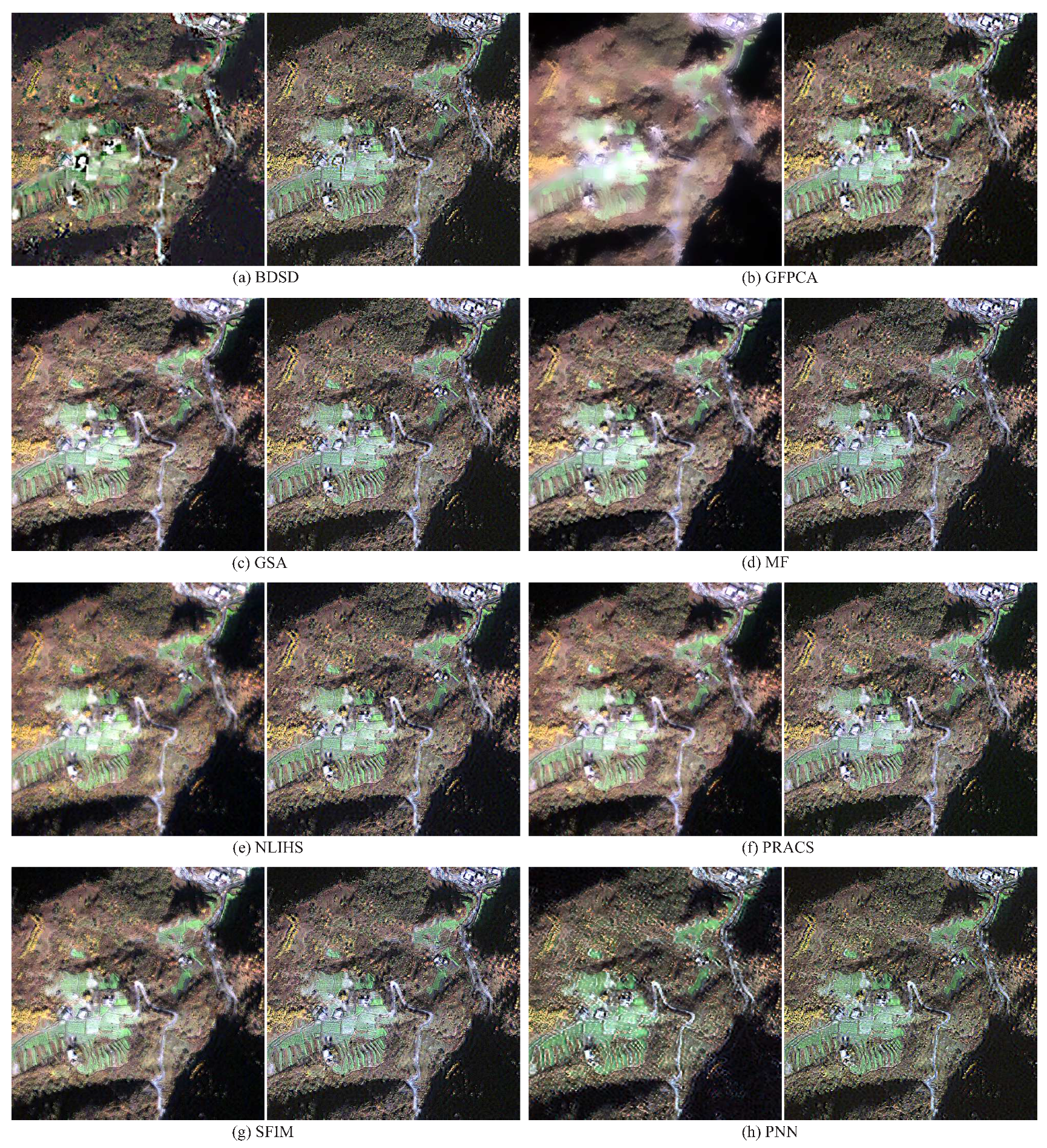
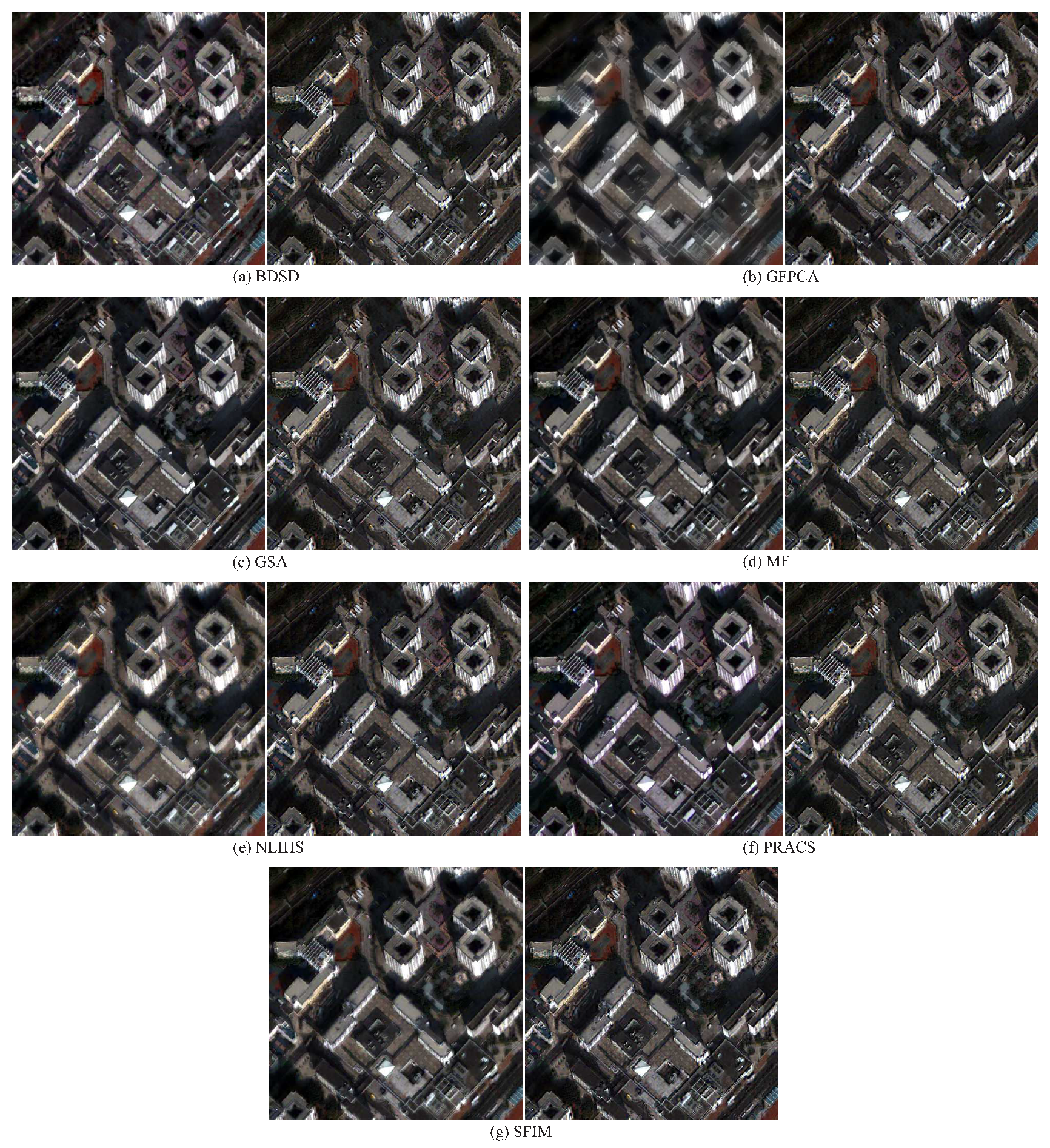
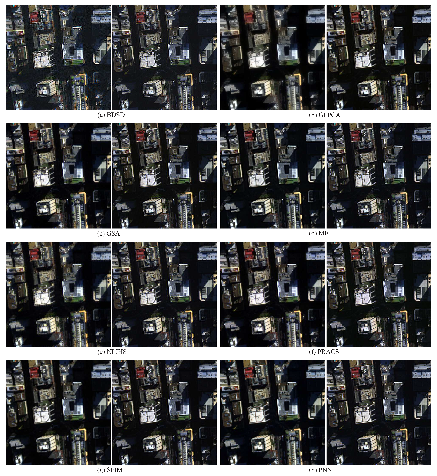
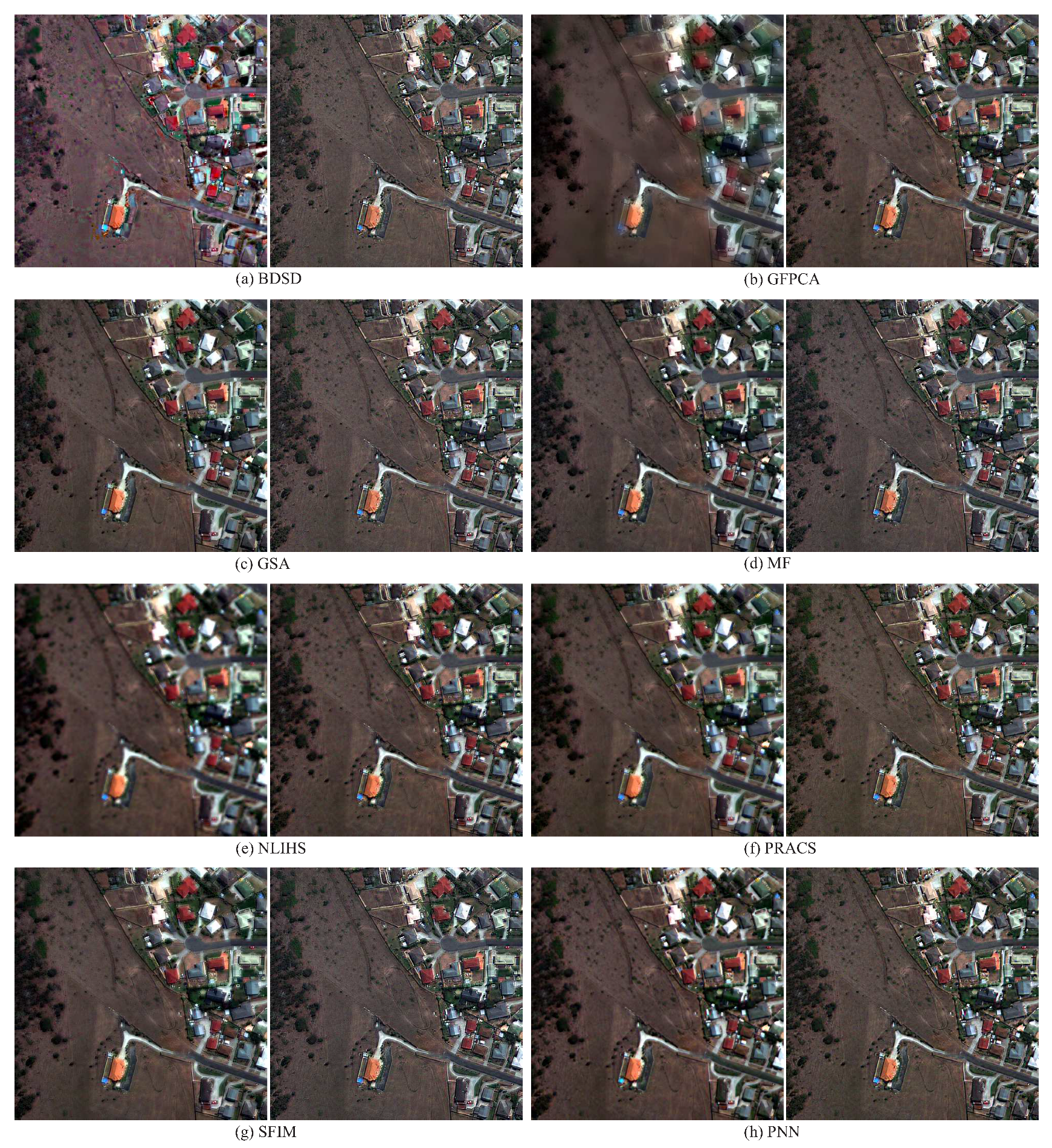
Visual Analysis. The pansharpened images on all the four datasets for the eight methods with and without our proposed EBP as postprocessing are shown in Figure 1, Figure 2, Figure 3 and Figure 4, where the RGB bands are displayed for visual comparison. It is worth noting that the conclusions are similar for both reduced and full scales. For the sake of brevity and the limitation of space, we don’t show the visual results at the reduced scale.
All the eight methods can effectively sharp the expanded MS image by bicubic interpolation as in their paper [11,12,13,18,19,20,24,35,63]. However, as one can see from these figures, the pansharpened images obtained by the eight methods with our proposed EBP as postprocessing, as shown on the right side of each subfigure, have better spatial and color quality than those of methods without EBP, as shown on the left side of each sugfigure. The proposed EBP can significantly improve the spatial details of the fused images obtained by other methods, this is clearly visible on the edges of the buildings, especially for GFPCA and NLIHS, which produce fused images with very strong blurring for the mountains in Figure 1 and the buildings in Figure 2 and Figure 3, as well as on the houses and ground surface in Figure 4. Although some methods such as BDSD can produce the better results with less blurring, they sometimes suffer from strong spectral distortions, as shown in Figure 4, the false RGB colors indicate that the results after postprocessing by our proposed EBP can preserve well the spectral information, as also confirmed by the following quantitative comparisons. As for the GSA, MF, PNN methods, although they have a good balance between the injected spatial details and the maintain of original spectral information, their results with the EBP postprocessing can obtain more spatial details and more pleasant colors that those of without EBP postprocessing, see the displays in Figure 1, Figure 2, Figure 3 and Figure 4 for comparisons.
As a summary of the visual analysis, the proposed EBP algorithm can significantly enhance the performances of other methods for improving the spatial details while presenting natural and pleasant visual results.
Quantitative Analysis. Quantitative evaluation further helps explaining the conclusions drawn from the visual analysis. The quantitative results by the considered metrics are provided as an objective evaluation. Specially, Table 2 reports the results for the four datasets obtained by eight benchmark methods with and without postprocessing by our proposed EBP at full scale. Besides, Table 3 presents the corresponding results by the aforementioned five numeric metrics at a reduced scale based on Wald’s protocol [49]. Note that the best result for each method with and without our proposed EBP as postprocessing is shown in boldface blue. According to the two tables, one can see that the eight benchmark methods produce fusion products that resulted in better quantitative scores for those five metrics at reduced scale and the three metrics at full scale when our proposed EBP algorithm was used for postprocessing, compared by those obtained without our proposed EBP as postprocessing, except that the original results of GFPCA and PRACS have a relatively better spectral quality (corresponding to the metrics ) for the IKONOS datasets and the NLIHS for the QuickBird dataset in the full scale experiments. As for the GeoEye-1 dataset in the full scale experiments, although the results of GSA, MF and NLIHS methods after postprocessing by our proposed EBP have a little bit precision loss in spectral quality, they have much better performances on the whole as shown by the value of the index QNR in Table 2. Another interesting observation, however, can be made for BDSD method on GeoEye-1 dataset in the full scale experiments. In this case, we find that the BDSD algorithm did not seem to benefit from the postprocessing, resulting in higher while lower QNR scores. This effect may be due to the severer spectral distortion of the fused products of BDSD as shown in Figure 4a. This reveals that additional attention must be taken when using the proposed method to process significantly spectral distortion images.
As for the reduced scale experiments, it is shown in Table 3 that the results of eight benchmark methods with our proposed EBP as postprocessing can almost always obtain the improved performances with the five metrics except for the PRACS method for the IKONOS and QuickBird datasets and the PNN method for the IKONOS dataset.
Overall, the results in Table 2 and Table 3 suggest that the use of our proposed EBP as postprocessing can be beneficial since a clear pattern of improvement based on visual inspection (as shown in Figure 1, Figure 2, Figure 3 and Figure 4) and quantitative comparison on five metrics at the reduced scale and three metrics at the full scale for four kinds of satellite datasets were observed for eight benchmark algorithms.
5. Conclusions
Pansharpening is an important preprocessing step for a variety of applications based on high resolution multispectral images. Over the past decades, lots of techniques, e.g., HM, HPM, the MTF-matched filter, and so on, have been proposed in this literature. However, the postprocessing for pansharpening has not received sufficient attention. Specifically, the integration of the HM, HPM and MTF-matched filter for pansharpening postprocessing is rarely investigated. In this paper, a post-processing method, called enhanced back-projection (EBP), which strives to integrate the HM, HPM and MTF-matched filters into the back-projection algorithm, is present and applied to pansharpening. Eight most benchmark pansharpening methods were selected and several experiments on four different kinds of satellite datasets were carried out to verify the effectiveness of the proposed EBP. The experimental results have shown that although our proposed EBP as postprocessing does not always guarantee better results, but it does frequently produce results that are equal to or better than the results without using our proposed EBP as postprocessing. Additionally, it should be noted that the proposed EBP as postprocessing works as an independent but complementary postprocessing module for pansharpening and thus does not need any modification of the existing pansharpening methods, which is a highly desirable feature. As is well-known, radiometric calibration (except the spectral and spatial) information is relevant to classification accuracy of remote sensing data. Thus, the studies on whether the radiometric calibration is maintained or lost after applying the post-processing pansharpening algorithm may be the focus of future studies.
Author Contributions
J.L., J.M. and R.F. conceived the experiments; J.L. and J.Z. structued and drafted the manuscript with assistance from H.L. and R.F.; J.M. and R.F. generated the graphics assisted by H.L.
Funding
This research was funded by the National Natural Science Foundation of China grant number 61877049, 61572393, 11671317, and 11601415.
Acknowledgments
The authors would like to thank Liao for sharing their codes of GFPCA in [24], to Giuseppe Scarpa for providing their codes of PNN in [41], to Gemine Vivone for sharing the pansharpening Matlab toolbox, and to the editors and the anonymous reviewers for their valuable comments and suggestions, which led to a substantial improvement of this paper.
Conflicts of Interest
The authors declare no conflict of interest.
References
- Shaw, G.; Burke, H.K. Spectral imaging for remote sensing. Linc. Lab. J. 2003, 14, 3–28. [Google Scholar]
- Bovolo, F.; Bruzzone, L.; Capobianco, L.; Garzelli, A.; Marchesi, S.; Nencini, F. Analysis of the effects of pansharpening in change detection on VHR image. IEEE Geosci. Remote Sens. Lett. 2010, 7, 53–57. [Google Scholar] [CrossRef]
- Xu, Y.; Smith, S.E.; Grunwald, S.; Abd-Elrahman, A.; Wani, S.P. Effects of image pansharpening on soil total nitrogen prediction models in South India. Geoderma 2018, 320, 52–66. [Google Scholar] [CrossRef]
- Laporterie-Déjean, F.; de Boissezon, H.; Flouzat, G.; Lefèvre-Fonollosa, M.-J. Thematic and statistical evaluations of five panchromatic/multispectral fusion methods on simulated PLEIADES-HR images. Inf. Fusion 2005, 6, 193–212. [Google Scholar] [CrossRef]
- Alparone, L.; Wald, L.; Chanussot, J.; Thomas, C.; Gamba, P.; Bruce, L.M. Comparison of pansharpening algorithms: Outcome of the 2006 GRS-S data-fusion contest. IEEE Trans. Geosci. Remote Sens. 2007, 45, 3012–3021. [Google Scholar] [CrossRef]
- Vivone, G.; Alparone, L.; Chanussot, J.; Mura, M.D.; Garzelli, A.; Licciardi, G.A.; Restaino, R.; Wald, L. A critical comparison among pansharpenig algorithms. IEEE Trans. Geosci. Remote Sens. 2015, 53, 2565–2586. [Google Scholar] [CrossRef]
- Aiazzi, B.; Alparone, L.; Baronti, S.; Carlà, R.; Garzelli, A.; Santurri, L. Sensitivity of pansharpening methods to temporal and instrumental changes between multispectral and panchromatic datasets. IEEE Trans. Geosci. Remote Sens. 2017, 55, 308–319. [Google Scholar] [CrossRef]
- Tu, T.; Su, S.; Shyu, H.; Huang, P. A new look at IHS-like image fusion methods. Inf. Fusion 2001, 2, 177–186. [Google Scholar] [CrossRef]
- Chavez, P.; Kwarteng, A. Extracting spectral contrast in Landsat thematic mapper image data using selective principal component analysis. Photogramm. Eng. Remote Sens. 1989, 55, 339–348. [Google Scholar]
- Laben, C.A.; Brower, B.V. Process for Enhancing the Spatial Resolution of Multispectral Imagery Using Pan-Sharpening. U.S. Patent 6011875, 4 January 2000. [Google Scholar]
- Aiazzi, B.; Baronti, S.; Selva, M. Improving component substitution pansharpening through multivariate regression of MS+Pan data. IEEE Trans. Geosci. Remote Sens. 2007, 45, 3230–3239. [Google Scholar] [CrossRef]
- Choi, J.; Yu, K.; Kim, Y. A new adaptive component-substitution-based satellite image fusion by using partial replacement. IEEE Trans. Geosci. Remote Sens. 2011, 49, 295–309. [Google Scholar] [CrossRef]
- Garzelli, A.; Nencini, F.; Capobianco, L. Optimal MMSE pan sharpening of very high resolution multispectral images. IEEE Trans. Geosci. Remote Sens. 2008, 46, 228–236. [Google Scholar] [CrossRef]
- Kang, X.; Li, S.; Benediktsson, J.A. Pansharpening with matting model. IEEE Trans. Geosci. Remote Sens. 2014, 52, 5088–5099. [Google Scholar] [CrossRef]
- Liu, J.; Liang, S. Pan-sharpening using a guided filter. Int. J. Remote Sens. 2016, 37, 1777–1800. [Google Scholar] [CrossRef]
- Leung, Y.; Liu, J.; Zhang, J. An improved adaptive intensity-hue-saturation method for the fusion of remote sensing images. IEEE Geosci. Remote Sens. Lett. 2014, 11, 985–989. [Google Scholar] [CrossRef]
- Schowengerdt, R.A. Remote Sensing: Models and Methods for Image Processing, 2nd ed.; Academic: Orlando, FL, USA, 1997. [Google Scholar]
- Liu, J.G. Smoothing filter based intensity modulation: A spectral preserve image fusion technique for improving spatial details. Int. J. Remote Sens. 2000, 21, 3461–3472. [Google Scholar] [CrossRef]
- Aiazzi, B.; Alparone, L.; Baronti, S.; Garzelli, A.; Selva, M. MTF-tailored multiscale fusion of high-resolution MS and Pan imagery. Photogramm. Eng. Remote Sens. 2006, 72, 591–596. [Google Scholar] [CrossRef]
- Restaino, R.; Vivone, G.; Mura, M.D.; Chanussot, J. Fusion of multispectral and panchromatic images based on morphological operators. IEEE Trans. Image Process. 2016, 25, 2882–2895. [Google Scholar] [CrossRef] [PubMed]
- Lee, J.; Lee, C. Fast and efficient panchromatic sharpening. IEEE Trans. Geosci. Remote Sens. 2010, 48, 155–163. [Google Scholar]
- Liu, J.; Hui, Y.; Zan, P. Locally linear detail injection for pansharpening. IEEE Access 2017, 5, 9728–9738. [Google Scholar] [CrossRef]
- Núñez, J.; Otazu, X.; Fors, O.; Prades, A.; Palà, V.; Arbiol, R. Multiresolution-based image fusion with additive wavelent decomposition. IEEE Trans. Geosci. Remote Sens. 1999, 37, 1204–1211. [Google Scholar] [CrossRef]
- Liao, W.; Huang, X.; van Coillie, F.; Gautama, S.; Pižurica, A.; Philips, W.; Liu, H.; Zhu, T.; Shimoni, M.; Moser, G.; et al. Processing of multiresolution thermal hyperspectral and digital color data: Outcome of the 2014 IEEE GRSS Data Fusion Contest. IEEE J. Sel. Top. Appl. Earth Obs. Remote Sens. 2015, 8, 2984–2996. [Google Scholar] [CrossRef]
- Shah, V.P.; Younan, N.H.; King, R.L. An efficient pan-sharpening method via a combined adaptive PCA approach and contourlets. IEEE Trans. Geosci. Remote Sens. 2008, 46, 1323–1335. [Google Scholar] [CrossRef]
- Smith, W.J. Chapter 15.8 The Modulation Transfer Function. In Modern Optical Engineering, 4th ed.; McGraw-Hill Education: New York, NY, USA, 2008; pp. 385–390. [Google Scholar]
- Aiazzi, B.; Baronti, S.; Lotti, F.; Selva, M. A comparison between global and context-adaptive pansharpening of multispectral images. IEEE Geosci. Remote Sens. Lett. 2009, 6, 302–306. [Google Scholar] [CrossRef]
- Li, Z.H.; Leung, H. Fusion of multispectral and panchromatic images using a restoration-based method. IEEE Trans. Geosci. Remot Sens. 2009, 46, 228–236. [Google Scholar]
- Palsson, F.; Sveinsson, J.R.; Ulfarsson, M.O. A new pansharpening algorithm based on total variation. IEEE Geosci. Remot Sens. Lett. 2014, 11, 318–322. [Google Scholar] [CrossRef]
- He, X.; Condat, L.; Bioucas-Dias, J.; Chanussot, J.; Xia, J. A new pansharpening method based on spatial and spectral sparsity priors. IEEE Trans. Image Process. 2014, 23, 4160–4174. [Google Scholar] [CrossRef]
- Li, S.; Yang, B. A new pansharpening method using a compressed sensing technique. IEEE Trans. Geosci. Remote Sens. 2011, 49, 738–746. [Google Scholar] [CrossRef]
- Zhu, X.X.; Bamler, R. A sparse image fusion algorithm with application to pan-sharpening. IEEE Trans. Geosci. Remote Sens. 2013, 51, 2827–2836. [Google Scholar] [CrossRef]
- Jiang, C.; Zhang, H.; Shen, H.; Zhang, L. Two-step sparse coding for the pan-sharpening of remote sensing images. IEEE Sel. Top. Appl. Earth Obs. Remote Sens. 2014, 7, 1792–1805. [Google Scholar] [CrossRef]
- Li, S.; Yin, H.; Fang, L. Remote sensing image fusion via sparse representations over learned dictionaries. IEEE Trans. Geosci. Remote Sens. 2013, 51, 4779–4789. [Google Scholar] [CrossRef]
- Vicinanza, M.R.; Restaino, R.; Vivone, G.; Mura, M.D.; Chanussot, J. A pansharpening method based on the sparse representation of injected details. IEEE Geosci. Remote Sens. Lett. 2015, 12, 180–184. [Google Scholar] [CrossRef]
- Zhu, X.X.; Grohnfeldt, C.; Bamler, R. Exploiting joint sparsity for pansharpening: The j-sparsefi algorithm. IEEE Trans. Geosci. Remote Sens. 2016, 54, 2664–2681. [Google Scholar] [CrossRef]
- Fasbender, D.; Radoux, J.; Bogaert, P. Bayesian data fusion for adaptable image pansharpening. IEEE Trans. Geosci. Remote Sens. 2008, 46, 1847–1857. [Google Scholar] [CrossRef]
- Zhu, X.; Tuia, D.; Mou, L.; Xia, G.; Zhang, L.; Xu, F.; Fraundorfer, F. Deep learning in remote sensing: A comprehensive review and list of resources. IEEE Geosci. Remote Sens. Mag. 2017, 5, 8–36. [Google Scholar] [CrossRef]
- Zhang, L.; Zhang, L.; Du, B. Deep learning for remote sensing data: A technical tutorial on the state of the art. IEEE Geosci. Remote Sens. Mag. 2016, 4, 22–40. [Google Scholar] [CrossRef]
- Huang, W.; Xiao, L.; Wei, Z.; Liu, H.; Tang, S. A new pan-sharpening method with deep neural networks. IEEE Geosci. Remote Sens. Lett. 2015, 12, 1037–1041. [Google Scholar] [CrossRef]
- Masi, G.; Cozzolino, D.; Verdoliva, L.; Scarpa, G. Pansharpening by convolutional neural networks. Remote Sens. 2016, 8, 594. [Google Scholar] [CrossRef]
- Wei, Y.; Yuan, Q.; Shen, H.; Zhang, L. Boosting the accuracy of multispectral image pansharpening by learning a deep residual network. IEEE Geosci. Remote Sens. Lett. 2017, 14, 1795–1799. [Google Scholar] [CrossRef]
- Loncan, L.; de Almeida, L.B.; Bioucas-Dias, J.M.; Briottet, X.; Chanussot, J.; Dobigeon, N.; Fabre, S.; Liao, W.; Licciardi, G.A.; Simoes, M.; et al. Hyperspectral pansharpening: A review. IEEE Geosci. Remote Sens. Mag. 2015, 3, 27–46. [Google Scholar] [CrossRef]
- Picone, D.; Restaino, R.; Vivone, G.; Addesso, P.; Dalla Mura, M.; Chanussot, J. Band assignment approaches for hyperspectral sharpening. IEEE Geosci. Remote Sens. Lett. 2017, 14, 739–743. [Google Scholar] [CrossRef]
- Alparone, L.; Garzelli, A.; Vivone, G. Intersensor statistical matching for pansharpening: Theoretical issues and practical solutions. IEEE Trans. Geosci. Remote Sens. 2017, 55, 4682–4695. [Google Scholar] [CrossRef]
- Xie, B.; Zhang, H.K.; Huang, B. Revealing implicit assumptions of the component substitution pansharpening methods. Remote Sens. 2017, 9, 443. [Google Scholar] [CrossRef]
- Vivone, G.; Restaino, R.; Mura, M.D.; Licciardi, G.; Chanussot, J. Contrast and error-based fusion schemes for multispectral image pansharpening. IEEE Geosci. Remote Sens. Lett. 2014, 11, 930–934. [Google Scholar] [CrossRef]
- Vivone, G.; Restaino, R.; Chanussot, J. A regression-based high-pass modulation pansharpening approach. IEEE Trans. Geosci. Remote Sens. 2018, 56, 984–996. [Google Scholar] [CrossRef]
- Wald, L.; Ranchin, T.; Mangolini, M. Fusion of satellite images of different spatial resolutions: Assessing the quality of resulting images. Photogramm. Eng. Remote Sens. 1997, 63, 691–699. [Google Scholar]
- Irani, M.; Peleg, S. Motion analysis for image enhancement: resolution, occlusion and transparency. J. Vis. Commun. Image Represent. 1993, 4, 324–335. [Google Scholar] [CrossRef]
- Haris, M.; Shakhnarovich, G.; Ukita, N. Deep back-projection networks for superresolution. arXiv, 2018; arXiv:1803.02735. [Google Scholar]
- Timofte, R.; Rothe, R.; Van Gool, L. Seven ways to improve example-based single image super resolution. In Proceedings of the IEEE Conference on Computer Vision and Pattern Recognition, Las Vegas, NV, USA, 27–30 June 2016; pp. 1865–1873. [Google Scholar]
- Wang, Z.; Zou, D.; Armenakis, C.; Li, D.; Li, Q. A comparative analysis of image fusion methods. IEEE Trans. Geosci. Remote Sens. 2005, 43, 1391–1402. [Google Scholar] [CrossRef] [Green Version]
- Kallel, A. MTF-adjust pansharpening approach based on coupled multiresolution decompositions. IEEE Trans. Geosci. Remote Sens. 2015, 53, 3124–3145. [Google Scholar] [CrossRef]
- Hallabia, H.; Kallel, A.; Ben Hamida, A.; Le Hegarat-Mascle, S. High spectral quality pansharpening approach based on MTF-matched filter banks. Multidimens. Syst. Signal Process. 2016, 27, 831–861. [Google Scholar] [CrossRef]
- Dai, S.; Han, M.; Wu, Y.; Gong, Y. Bilateral back-projection for single image super resolution. In Proceedings of the 2007 IEEE International Conference on Multimedia and Expo (ICME’07), Beijing, China, 2–5 July 2007; pp. 1039–1042. [Google Scholar]
- Irani, M.; Peleg, S. Improving resolutin by image registration. CVGIP Graph. Models Image Process. 1991, 53, 231–239. [Google Scholar] [CrossRef]
- Zhao, Y.; Wang, R.; Jia, W.; Wang, W.; Gao, W. Iterative projection reconstruction for fast and efficient image upsampling. Neurocomputing 2017, 226, 200–211. [Google Scholar] [CrossRef]
- Haris, M.; Widyanto, M.R.; Nobuhara, H. First-order derivative-based super-resolution. Signal Image Video Process. 2017, 11, 1–8. [Google Scholar] [CrossRef]
- Dong, W.; Zhang, L.; Shi, G.; Wu, X. Nonlocal back-projection for adaptive image enlargement. In Proceedings of the 2009 16th IEEE International Conference on Image Processing (ICIP), Cairo, Egypt, 7–10 November 2009; pp. 349–352. [Google Scholar]
- Yang, J.; Wright, J.; Huang, T.; Ma, Y. Image super-resolution via sparse representation. IEEE Trans. Image Process. 2010, 19, 2861–2873. [Google Scholar] [CrossRef]
- Selva, M.; Santurri, L.; Baronti, S. On the use of the expanded image in quality assessment of pansharpening images. IEEE Geosci. Remote Sens. Lett. 2018, 15, 320–324. [Google Scholar] [CrossRef]
- Ghahremani, M.; Ghassemian, H. Nonlinear IHS: A promising method for pan-sharpening. IEEE Geosci. Remote Sens. Lett. 2016, 13, 1606–1610. [Google Scholar] [CrossRef]
- Alparone, L.; Aiazzi, B.; Baronti, S.; Garzelli, A.; Nencini, F.; Selva, M. Multispectral and panchromatic data fusion assessment without reference. Photogramm. Eng. Remote Sens. 2008, 74, 193–200. [Google Scholar] [CrossRef]
- Yocky, D. Multiresolution wavelet decomposition image merger of Landsat Thematic Mapper and SPOT panchromatic data. Photogramm. Eng. Remote Sens. 1996, 62, 1067–1074. [Google Scholar]
- Wald, L. Quality of high resolution synthesised images: Is there a simple criterion? In Proceedings of the Third Conferences on Fusion of Earth Data: Merging Point Measurements, Raster Maps and Remotely Sensed Images, Sophia Antipolis, France, 26–28 January 2000; pp. 99–103. [Google Scholar]
- Yuhas, R.; Boardman, J. Discrimination among semi-arid landscape endmembers using the Spectral Angle Mapper (sam) algorithm. In Proceedings of the 3rd Annual JPL Airborne Geoscience Workshop, JPL Publication, Pasadena, CA, USA, 1–5 June 1992; pp. 147–149. [Google Scholar]
- Alparone, L.; Baronti, S.; Garzelli, A.; Nencini, F. A global quality measurement of pan-sharpened multispectral imagery. IEEE Geosci. Remote Sens. Lett. 2004, 1, 313–317. [Google Scholar] [CrossRef]
- Garzelli, A.; Nencini, F. Hypercomplex quality assessment of multi/hyperspectral images. IEEE Geosci. Remote Sens. Lett. 2009, 6, 662–665. [Google Scholar] [CrossRef]
- Wang, Z.; Bovik, A.C. A universal image quality index. IEEE Signal Process. Lett. 2002, 9, 81–84. [Google Scholar] [CrossRef]
Figure 1.
Visual comparison of the fused images obtained by eight methods with and without the proposed EBP as postprocessing on the IKONOS dataset, (a) BDSD; (b) GFPCA; (c) GSA; (d) MF; (e) NLIHS; (f) PRACS; (g) SFIM; (h) PNN. In contrast, the results with EBP postprocessing (on the right side of each subfigure) have more spatial details and more pleasant colors than those of without EBP (on the left side of each subfigure). Best zoomed in on screen for visual comparison.

Figure 2.
Visual comparison of the fused images obtained by eight methods with and without the proposed EBP as postprocessing on the QuickBird dataset, (a) BDSD; (b) GFPCA; (c) GSA; (d) MF; (e) NLIHS; (f) PRACS; (g) SFIM. In contrast, the results with EBP postprocessing (on the right side of each subfigure) have more spatial details and more pleasant colors than those of without EBP (on the left side of each subfigure). Best zoomed in on screen for visual comparison.

Figure 3.
Visual comparison of the fused images obtained by eight methods with and without the proposed EBP as postprocessing on the WorldView-2 dataset, (a) BDSD; (b) GFPCA; (c) GSA; (d) MF; (e) NLIHS; (f) PRACS; (g) SFIM; (h) PNN. In contrast, the results with EBP postprocessing (on the right side of each subfigure) have more spatial details and more pleasant colors than those of without EBP (on the left side of each subfigure). Best zoomed in on screen for visual comparison.

Figure 4.
Visual comparison of the fused images obtained by eight methods with and without the proposed EBP as postprocessing on the GeoEye-1 dataset, (a) BDSD; (b) GFPCA; (c) GSA; (d) MF; (e) NLIHS; (f) PRACS; (g) SFIM; (h) PNN. In contrast, the results with EBP postprocessing (on the right side of each subfigure) have more spatial details and more pleasant colors than those of without EBP (on the left side of each subfigure). Best zoomed in on screen for visual comparison.


Table 1.
Parameters of different satellites. Note that the gains at Nyquist cutoff frequency of the MTFs (MTF gain) are reported in parentheses and in blue.
Table 1.
Parameters of different satellites. Note that the gains at Nyquist cutoff frequency of the MTFs (MTF gain) are reported in parentheses and in blue.
| Parameters | IKONOS | QuickBird | WorldView-2 | GeoEye-1 | |
|---|---|---|---|---|---|
| Launch date | 24 September 1999 | 18 October 2001 | 8 October 2009 | 6 September 2008 | |
| Temporal resolution | <3 days | 1–5 days | 1.1 day | <3 days | |
| Radiometric resolution | 11 | 11 | 11 | 11 | |
| Spatial resolution | MS | 4 m | 2.4 m | 1.84 m | 1.84 m |
| PAN | 1 m | 0.6 m | 0.46 m | 0.46 m | |
| Spectral range (MTF gain) | Blue | 445–516 nm (0.27) | 450–520 nm (0.34) | 450–510 nm (0.35) | 450–510 nm (0.23) |
| Green | 506–595 nm (0.28) | 520–600 nm (0.32) | 510–580 nm (0.35) | 510–580 nm (0.23) | |
| Red | 632–698 nm (0.29) | 630–690 nm (0.30) | 630–690 nm (0.35) | 655–690 nm (0.23) | |
| NIR1 | 757–900 nm (0.28) | 760–900 nm (0.22) | 770–895 nm (0.35) | 780–920 nm (0.23) | |
| Red edge | 705–745 nm (0.35) | ||||
| Coastal | 400–450 nm (0.35) | ||||
| Yellow | 585–625 nm (0.27) | ||||
| NIR2 | 860–1040 nm (0.35) | ||||
| PAN | 450–900 nm (0.17) | 450–900 nm (0.15) | 450–800 nm (0.11) | 450–800 nm (0.16) |
Table 2.
Quantitative comparison for the eight methods without (denoted by ✗ ) and with (denoted by ✓) postprocessing by our proposed EBP on four kinds of satellite datasets in the full scale. Note that, for better comparison, the results improved by EBP are highlighted in blue, otherwise the original results are colored in green.
| Datasets | Metrics | EBP | BDSD | GFPCA | GSA | MF | NLIHS | PRACS | SFIM | PNN |
|---|---|---|---|---|---|---|---|---|---|---|
| IKONOS | ✗ | 0.010 | 0.020 | 0.054 | 0.041 | 0.028 | 0.021 | 0.034 | 0.082 | |
| ✓ | 0.010 | 0.041 | 0.030 | 0.022 | 0.012 | 0.028 | 0.021 | 0.020 | ||
| ✗ | 0.066 | 0.129 | 0.454 | 0.244 | 0.103 | 0.236 | 0.143 | 0.242 | ||
| ✓ | 0.062 | 0.056 | 0.171 | 0.152 | 0.116 | 0.119 | 0.141 | 0.123 | ||
| QNR | ✗ | 0.925 | 0.854 | 0.517 | 0.724 | 0.872 | 0.748 | 0.828 | 0.696 | |
| ✓ | 0.928 | 0.906 | 0.804 | 0.830 | 0.873 | 0.856 | 0.841 | 0.859 | ||
| QuickBird | ✗ | 0.039 | 0.035 | 0.031 | 0.035 | 0.006 | 0.037 | 0.021 | - | |
| ✓ | 0.019 | 0.020 | 0.013 | 0.010 | 0.011 | 0.025 | 0.009 | - | ||
| ✗ | 0.022 | 0.079 | 0.065 | 0.036 | 0.060 | 0.061 | 0.025 | - | ||
| ✓ | 0.020 | 0.024 | 0.018 | 0.027 | 0.022 | 0.019 | 0.020 | - | ||
| QNR | ✗ | 0.940 | 0.889 | 0.907 | 0.930 | 0.935 | 0.904 | 0.954 | - | |
| ✓ | 0.962 | 0.957 | 0.969 | 0.962 | 0.967 | 0.956 | 0.972 | - | ||
| WorldView-2 | ✗ | 0.033 | 0.037 | 0.009 | 0.015 | 0.009 | 0.013 | 0.009 | 0.028 | |
| ✓ | 0.006 | 0.010 | 0.008 | 0.007 | 0.009 | 0.018 | 0.005 | 0.013 | ||
| ✗ | 0.092 | 0.048 | 0.044 | 0.017 | 0.038 | 0.039 | 0.026 | 0.030 | ||
| ✓ | 0.045 | 0.012 | 0.009 | 0.015 | 0.004 | 0.009 | 0.006 | 0.011 | ||
| QNR | ✗ | 0.878 | 0.916 | 0.947 | 0.969 | 0.953 | 0.948 | 0.965 | 0.943 | |
| ✓ | 0.949 | 0.978 | 0.982 | 0.979 | 0.987 | 0.973 | 0.989 | 0.976 | ||
| GeoEye-1 | ✗ | 0.200 | 0.126 | 0.111 | 0.163 | 0.004 | 0.035 | 0.177 | 0.037 | |
| ✓ | 0.228 | 0.102 | 0.154 | 0.174 | 0.007 | 0.025 | 0.175 | 0.036 | ||
| ✗ | 0.056 | 0.125 | 0.172 | 0.155 | 0.055 | 0.116 | 0.139 | 0.051 | ||
| ✓ | 0.031 | 0.080 | 0.034 | 0.035 | 0.051 | 0.081 | 0.037 | 0.038 | ||
| QNR | ✗ | 0.755 | 0.765 | 0.736 | 0.708 | 0.941 | 0.853 | 0.709 | 0.914 | |
| ✓ | 0.748 | 0.827 | 0.817 | 0.797 | 0.942 | 0.896 | 0.794 | 0.927 |
Table 3.
Quantitative comparison for the eight methods without (denoted by ✗) and with (denoted by ✓) postprocessing by our proposed EBP on four kinds of satellite datasets in the reduced scale. Note that, for better comparison, the results improved by EBP are highlighted in blue, otherwise the original results are colored in green.
| Datasets | Metrics | EBP | BDSD | GFPCA | MF | GSA | NLIHS | PRACS | SFIM | PNN |
|---|---|---|---|---|---|---|---|---|---|---|
| IKONOS | CC | ✗ | 0.923 | 0.916 | 0.937 | 0.933 | 0.922 | 0.946 | 0.942 | 0.931 |
| ✓ | 0.940 | 0.948 | 0.941 | 0.939 | 0.930 | 0.943 | 0.942 | 0.937 | ||
| ERGAS | ✗ | 3.234 | 3.620 | 3.051 | 3.016 | 3.372 | 2.887 | 3.019 | 2.906 | |
| ✓ | 2.878 | 2.592 | 2.730 | 2.773 | 2.733 | 2.704 | 2.703 | 3.038 | ||
| SAM | ✗ | 3.989 | 4.429 | 3.599 | 3.773 | 4.323 | 3.523 | 3.663 | 3.572 | |
| ✓ | 3.155 | 3.082 | 3.017 | 3.125 | 3.244 | 3.111 | 3.071 | 3.429 | ||
| RMSE | ✗ | 21.43 | 23.93 | 20.19 | 19.99 | 22.45 | 19.05 | 19.89 | 19.21 | |
| ✓ | 19.16 | 17.32 | 18.22 | 18.48 | 18.65 | 18.13 | 18.04 | 19.99 | ||
| Q4 | ✗ | 0.854 | 0.768 | 0.860 | 0.832 | 0.815 | 0.873 | 0.862 | 0.843 | |
| ✓ | 0.876 | 0.884 | 0.878 | 0.858 | 0.854 | 0.879 | 0.878 | 0.860 | ||
| QuickBird | CC | ✗ | 0.846 | 0.917 | 0.929 | 0.938 | 0.926 | 0.945 | 0.931 | - |
| ✓ | 0.928 | 0.954 | 0.949 | 0.945 | 0.949 | 0.940 | 0.947 | - | ||
| ERGAS | ✗ | 3.945 | 3.923 | 2.912 | 2.816 | 3.517 | 2.626 | 3.080 | - | |
| ✓ | 3.214 | 2.309 | 2.509 | 2.615 | 2.385 | 2.773 | 2.471 | - | ||
| SAM | ✗ | 4.391 | 3.444 | 2.514 | 2.942 | 2.981 | 2.796 | 2.649 | - | |
| ✓ | 2.269 | 2.089 | 2.090 | 2.187 | 2.183 | 2.269 | 2.144 | - | ||
| RMSE | ✗ | 55.55 | 53.29 | 39.64 | 38.47 | 47.48 | 36.20 | 41.70 | - | |
| ✓ | 44.14 | 31.71 | 34.43 | 35.90 | 33.06 | 38.78 | 33.94 | - | ||
| Q4 | ✗ | 0.838 | 0.755 | 0.904 | 0.891 | 0.834 | 0.912 | 0.882 | - | |
| ✓ | 0.902 | 0.933 | 0.932 | 0.924 | 0.930 | 0.917 | 0.929 | - | ||
| WorldView-2 | CC | ✗ | 0.868 | 0.947 | 0.964 | 0.972 | 0.961 | 0.975 | 0.965 | 0.974 |
| ✓ | 0.954 | 0.985 | 0.984 | 0.985 | 0.984 | 0.985 | 0.984 | 0.983 | ||
| ERGAS | ✗ | 11.481 | 7.534 | 4.863 | 4.939 | 6.383 | 4.625 | 5.297 | 4.332 | |
| ✓ | 6.601 | 3.138 | 3.348 | 3.057 | 2.990 | 3.201 | 3.213 | 3.375 | ||
| SAM | ✗ | 12.179 | 5.547 | 3.476 | 3.879 | 4.692 | 3.881 | 3.736 | 4.542 | |
| ✓ | 5.152 | 2.702 | 2.899 | 2.763 | 3.039 | 3.161 | 2.909 | 3.163 | ||
| RMSE | ✗ | 121.64 | 79.62 | 51.80 | 52.12 | 66.92 | 45.97 | 56.01 | 46.36 | |
| ✓ | 70.03 | 33.16 | 35.37 | 32.37 | 32.40 | 35.16 | 33.99 | 35.43 | ||
| Q8 | ✗ | 0.860 | 0.847 | 0.953 | 0.947 | 0.908 | 0.958 | 0.937 | 0.965 | |
| ✓ | 0.939 | 0.979 | 0.979 | 0.981 | 0.979 | 0.980 | 0.979 | 0.978 | ||
| GeoEye-1 | CC | ✗ | 0.852 | 0.795 | 0.894 | 0.863 | 0.875 | 0.890 | 0.892 | 0.908 |
| ✓ | 0.903 | 0.922 | 0.912 | 0.914 | 0.917 | 0.921 | 0.910 | 0.918 | ||
| ERGAS | ✗ | 3.724 | 4.309 | 2.982 | 3.278 | 3.586 | 3.177 | 3.157 | 2.783 | |
| ✓ | 3.002 | 2.539 | 2.706 | 2.676 | 2.592 | 2.515 | 2.707 | 2.623 | ||
| SAM | ✗ | 5.276 | 5.152 | 3.920 | 4.661 | 4.018 | 3.848 | 3.943 | 3.591 | |
| ✓ | 3.549 | 3.389 | 3.411 | 3.517 | 3.444 | 3.421 | 3.429 | 3.422 | ||
| RMSE | ✗ | 34.82 | 39.86 | 27.74 | 30.59 | 32.81 | 29.86 | 29.21 | 25.95 | |
| ✓ | 27.97 | 23.73 | 25.33 | 25.06 | 24.27 | 23.63 | 25.30 | 24.41 | ||
| Q4 | ✗ | 0.833 | 0.573 | 0.823 | 0.796 | 0.722 | 0.781 | 0.790 | 0.842 | |
| ✓ | 0.875 | 0.882 | 0.875 | 0.884 | 0.871 | 0.883 | 0.868 | 0.880 |
© 2019 by the authors. Licensee MDPI, Basel, Switzerland. This article is an open access article distributed under the terms and conditions of the Creative Commons Attribution (CC BY) license (http://creativecommons.org/licenses/by/4.0/).
Share and Cite
MDPI and ACS Style
Liu, J.; Ma, J.; Fei, R.; Li, H.; Zhang, J. Enhanced Back-Projection as Postprocessing for Pansharpening. Remote Sens. 2019, 11, 712. https://0-doi-org.brum.beds.ac.uk/10.3390/rs11060712
AMA Style
Liu J, Ma J, Fei R, Li H, Zhang J. Enhanced Back-Projection as Postprocessing for Pansharpening. Remote Sensing. 2019; 11(6):712. https://0-doi-org.brum.beds.ac.uk/10.3390/rs11060712
Chicago/Turabian StyleLiu, Junmin, Jing Ma, Rongrong Fei, Huirong Li, and Jiangshe Zhang. 2019. "Enhanced Back-Projection as Postprocessing for Pansharpening" Remote Sensing 11, no. 6: 712. https://0-doi-org.brum.beds.ac.uk/10.3390/rs11060712
Note that from the first issue of 2016, this journal uses article numbers instead of page numbers. See further details here.