Extraction of Urban Objects in Cloud Shadows on the basis of Fusion of Airborne LiDAR and Hyperspectral Data


1
College of Geography and Environment, Shandong Normal University, Jinan 250014, China
2
Department of Geography and the Environment, University of North Texas, Denton, TX 76203, USA
*
Author to whom correspondence should be addressed.
Remote Sens. 2019, 11(6), 713; https://0-doi-org.brum.beds.ac.uk/10.3390/rs11060713
Submission received: 1 February 2019
/
Revised: 20 March 2019
/
Accepted: 22 March 2019
/
Published: 25 March 2019
(This article belongs to the Special Issue Hyperspectral Imagery for Urban Environment)
Abstract
:Feature extraction in cloud shadows is a difficult problem in the field of optical remote sensing. The key to solving this problem is to improve the accuracy of classification algorithms by fusing multi-source remotely sensed data. Hyperspectral data have rich spectral information but highly suffer from cloud shadows, whereas light detection and ranging (LiDAR) data can be acquired from beneath clouds to provide accurate height information. In this study, fused airborne LiDAR and hyperspectral data were used to extract urban objects in cloud shadows using the following steps: (1) a series of LiDAR and hyperspectral metrics were extracted and selected; (2) cloud shadows were extracted; (3) the new proposed approach was used by combining a pixel-based support vector machine (SVM) and object-based classifiers to extract urban objects in cloud shadows; (4) a pixel-based SVM classifier was used for the classification of the whole study area with the selected metrics; (5) a decision-fusion strategy was employed to get the final results for the whole study area; (6) accuracy assessment was conducted. Compared with the SVM classification results, the decision-fusion results of the combined SVM and object-based classifiers show that the overall classification accuracy is improved by 5.00% (from 87.30% to 92.30%). The experimental results confirm that the proposed method is very effective for urban object extraction in cloud shadows and thus improve urban applications such as urban green land management, land use analysis, and impervious surface assessment.
1. Introduction
With the acceleration of urbanization, the problems of urban population expansion, resource shortage and traffic congestion are becoming increasingly serious. The trend in urban development is the increasing construction of smart cities according to appropriate spatial information, thereby improving the efficiency of urban management. The ability to acquire information about urban objects quickly and accurately is an important factor to ensure the smooth progress of intelligent cities. With the advantages of providing a synoptic view and rich spatial and spectral information, remote sensing can accurately obtain urban object information at various scales [1,2,3,4,5,6,7,8,9], and is becoming one of the most effective tools for urban object extraction [10].
Up to now, many scholars have carried out relevant studies on the extraction of urban objects with medium- and high-resolution optical images. With the accelerating process of urbanization, the types of urban objects are becoming increasingly complex, which makes urban object extraction more challenging. Examples of such challenges are as follows: (1) similar spectral characteristics are shared by many different urban land types, such as cement pavements, parking_lots, roads, rooftops, sidewalks, and buildings. Remote sensing data from a single source cannot meet the needs of current remote sensing applications [11,12]; (2) high-resolution optical remote sensing images may encounter serious problems with shadows, such as building shadows and cloud shadows; (3) medium-resolution optical remote sensing images have the mixed pixel problem; (4) the acquisition of optical remote sensing images is easily affected by the weather, which leads to weak spectral information in shadow areas. To overcome these limitations of single-source remote sensing data, studies have been carried out on urban object extraction that is based on multi-source remote sensing data [7,8,9,13].
With the continuous development of sensor technology, we can obtain different remote sensing images more conveniently and quickly, and this provides a prerequisite for multi-source image data fusion. Airborne hyperspectral data can acquire hundreds of continuous spectral bands that can provide the precise spectral information of land objects [14]. High-density light detection and ranging (LiDAR) point cloud data can provide precise height information [15]. These two data sources are complementary to each other, so their combination is very helpful for obtaining spectral and height information classification [16]. Up to now, many scholars have applied fused airborne LiDAR and hyperspectral data in various studies for a variety of purposes such as tree species classification [17,18,19,20,21], forest biomass estimation [22,23,24,25], and urban object extraction [26,27,28,29,30,31,32,33,34,35,36]. These studies have mainly concentrated on the following aspects: (1) Extraction of feature parameters, such as attribute profile parameters [26] and morphological attribute profile [27]. (2) Fusion methods, such as pixel-level [28,29,30,31,32], feature-level [27,30,33], and decision-level fusion [34,35,36,37]. Among them, pixel-level fusion mainly uses layer stacked feature parameters. Luo et al. [31] fused LiDAR and hyperspectral data by layer stacking, and they employed the maximum likelihood and support vector machine (SVM) classifiers to classify urban objects. Compared with the classification results of hyperspectral data alone, the overall accuracy of layer stacking fused hyperspectral and LiDAR data was improved by about 9.00%. Feature-level fusion is a method in which features are derived first, and comprehensive analysis and processing are then carried out. Man et al. [30] proposed new methods to fuse LiDAR and hyperspectral data in pixel-level and feature-level fusion, and they used object-based and SVM classifiers to extract urban land use information. In comparison with hyperspectral data alone, hyperspectral-LiDAR data fusion improved the overall accuracy by 6.80% (from 81.70% to 88.50%) when the SVM classifier was used. Meanwhile, compared with the SVM classifier alone, the combined SVM and object-based method improved the overall accuracy by 7.10% (from 87.60% to 94.70%). Zhang et al. [27] fused LiDAR and hyperspectral data in feature-level fusion, and improved the overall accuracy from 80.49% to 89.93% in comparison with hyperspectral data alone. Decision level fusion is used to classify and identify each image individually, and then get the optimal decision results. Zhong et al. [36] fused LiDAR and hyperspectral data in decision-level fusion, and improved the overall accuracy from 87.80% to 90.80% when compared with hyperspectral data alone. Bigdeli et al. [34] applied a decision-fusion method based on multiple support vector machine system for fusing hyperspectral and LiDAR data, the overall accuracy was improved from 88.00% to 91.00% in comparison with hyperspectral data alone. (3) Classification methods have included spectral angle mapping [28], random forest [32,38,39], maximum likelihood classification [28,29,31,33,36,40], support vector machine [29,31,34,36,38,39,40], and object-based classification [41,42]. In general, many studies have shown that LiDAR and hyperspectral data fusion could overcome some of the limitations of using a single data source for object extraction [43].
Although many studies have fused LiDAR and hyperspectral data for urban object extraction and obtained improved classification results [31], there are still some problems that need to be further investigated. For example, few studies have focused on urban object extraction in shadows by using hyperspectral and LiDAR data. Against the background of accelerated urbanization, it is essential to make full use of the advantages of multi-source remotely sensed data to improve the overall accuracy of urban object extraction and support intelligent cities and urban planning activities. While the pixel-based SVM classifier works well with high-dimensional data classification, it is difficult to achieve high classification accuracy using the pixel-based SVM classifier in shadow areas because of missing spectral information. Besides that, the advantage of LiDAR height information is not fully utilized. Therefore, there is a need to explore other methods for fusing LiDAR and hyperspectral data. Object-based classification is an evolving technology that is driven by the understanding of objects rather than pixels [44]. This study aims to extract urban objects in shadows using fused airborne LiDAR and hyperspectral data, and utilizes the advantages of LiDAR data in shadows to improve the overall accuracy of urban object extraction. We propose a new workflow to fuse hyperspectral and LiDAR data for the classification of remotely sensed scenes with cloud shadows. The proposed method comprises the following steps. Firstly, cloud shadow areas are extracted. Secondly, a multi-scale object-based classification method is used to classify cloud shadow areas. Thirdly, the whole study area is classified with pixel-based support vector machine algorithms. Finally, decision-level fusion is conducted to improve the overall classification accuracy of the whole study area, including the cloud shadow areas.
2. Study Area and Data
2.1. Study Site
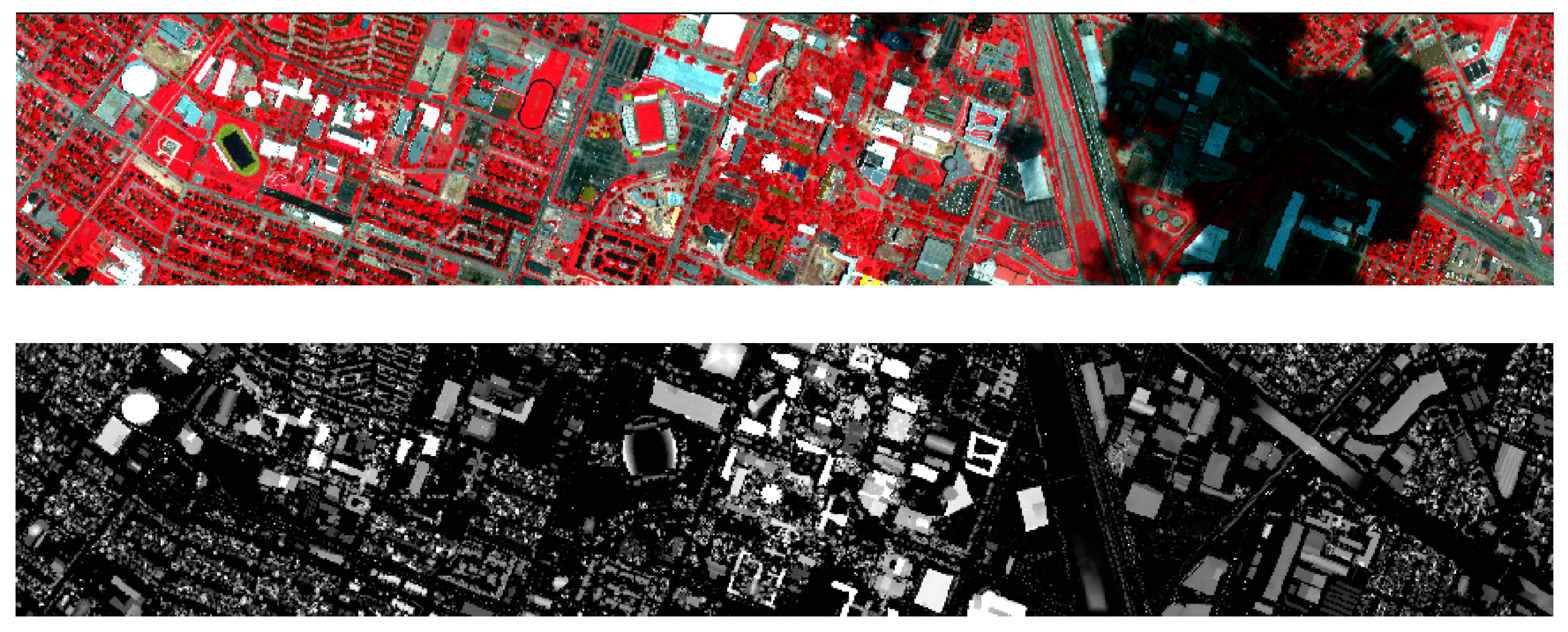
The study area is in Houston in the southeast of Texas, USA (Figure 1), covering an area of approximately 4 km2, extending from 95°19′13.56″W to 95°22′9.94″W and 29°43′0.96″N to 29°43′32.34″N.
2.2. Datasets
The datasets used in this study are provided by the 2013 IEEE GRSS Data Fusion Contest [43] (URL: http://www.grssieee.org/community/technical-commitees/data-fusion/) and include airborne hyperspectral imagery, LiDAR point cloud data, training data and validation data.
2.2.1. LiDAR Data
The LiDAR data used in the present study were acquired on 22 June 2012 between the times 14:37:55 and 15:38:10 UTC (Coordinated Universal Time). The sensor recorded five returns and intensity information at a platform altitude of 609.6 m, with an average point spacing of 0.74 m. In this study, the intensity of LiDAR data was not calibrated, and the atmospheric effects were not considered.
2.2.2. Hyperspectral Data
The hyperspectral imagery data were acquired on 23 June 2012 between the times of 17:37:10 and 17:39:50 UTC. The sensor is CASI and its above ground height is 1676.4 m. There are 144 spectral bands in the 380-1050 nm region. The hyperspectral imagery was calibrated to at-sensor spectral radiance units (SRUs), which are equivalent to units of μWcm−2sr−1nm−1. The spectral and spatial resolutions were 4.8 nm and 2.5 m, respectively.
2.2.3. Training and Validation Data
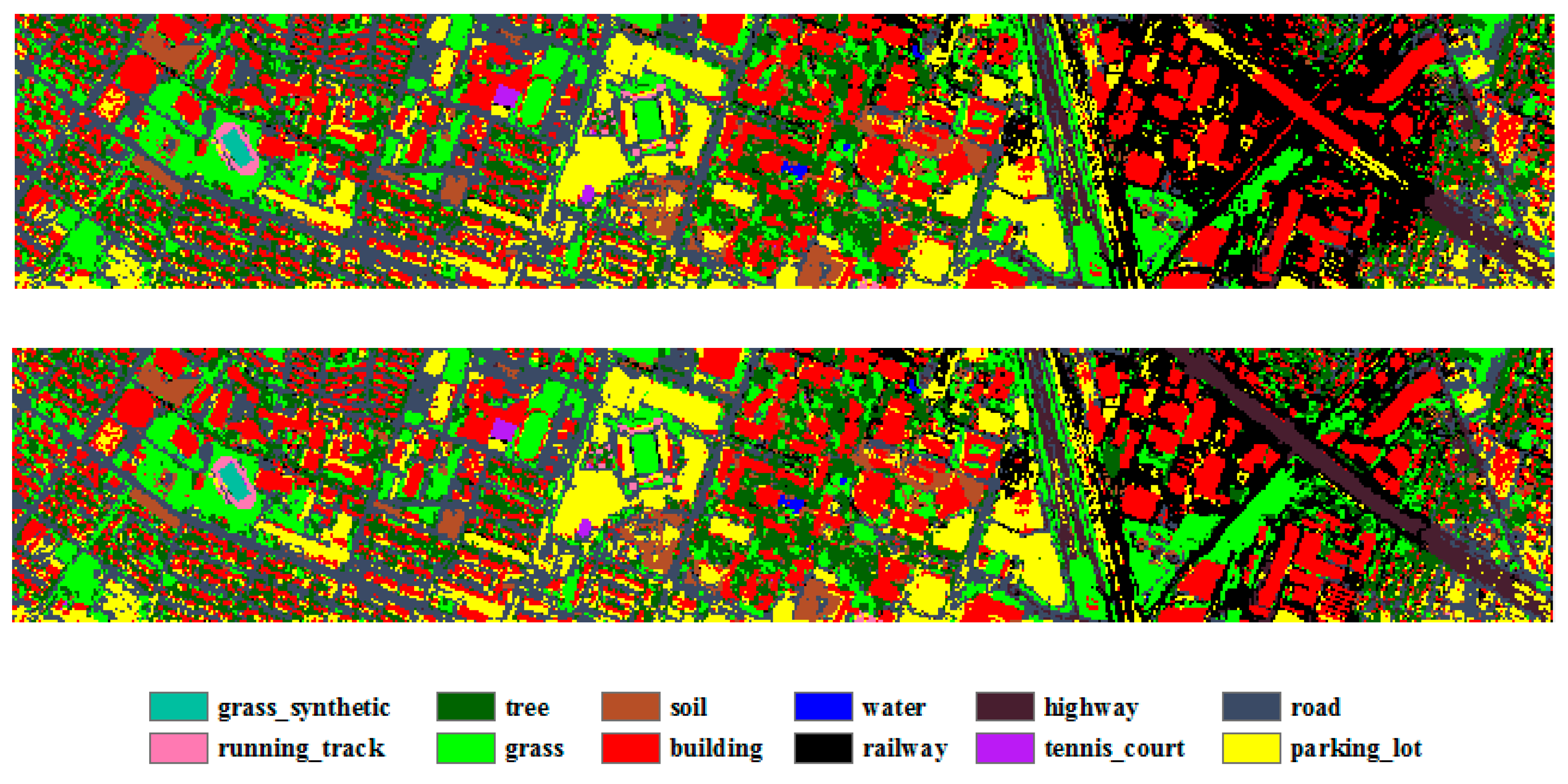
In this study, 12 classes were identified: (1) grass; (2) grass_synthetic; (3) road; (4) soil; (5) railway; (6) parking_lot; (7) tennis_court; (8) running_track; (9) water; (10) trees; (11) building; and (12) highway. Training and validation samples for classification were both provided by the 2013 IEEE GRSS Data Fusion Contest [43] (URL: http://www.grss-ieee.org/community/technical-commitees/data-fusion/). Table 1 shows detailed information on the training and validation samples.
3. Methodology
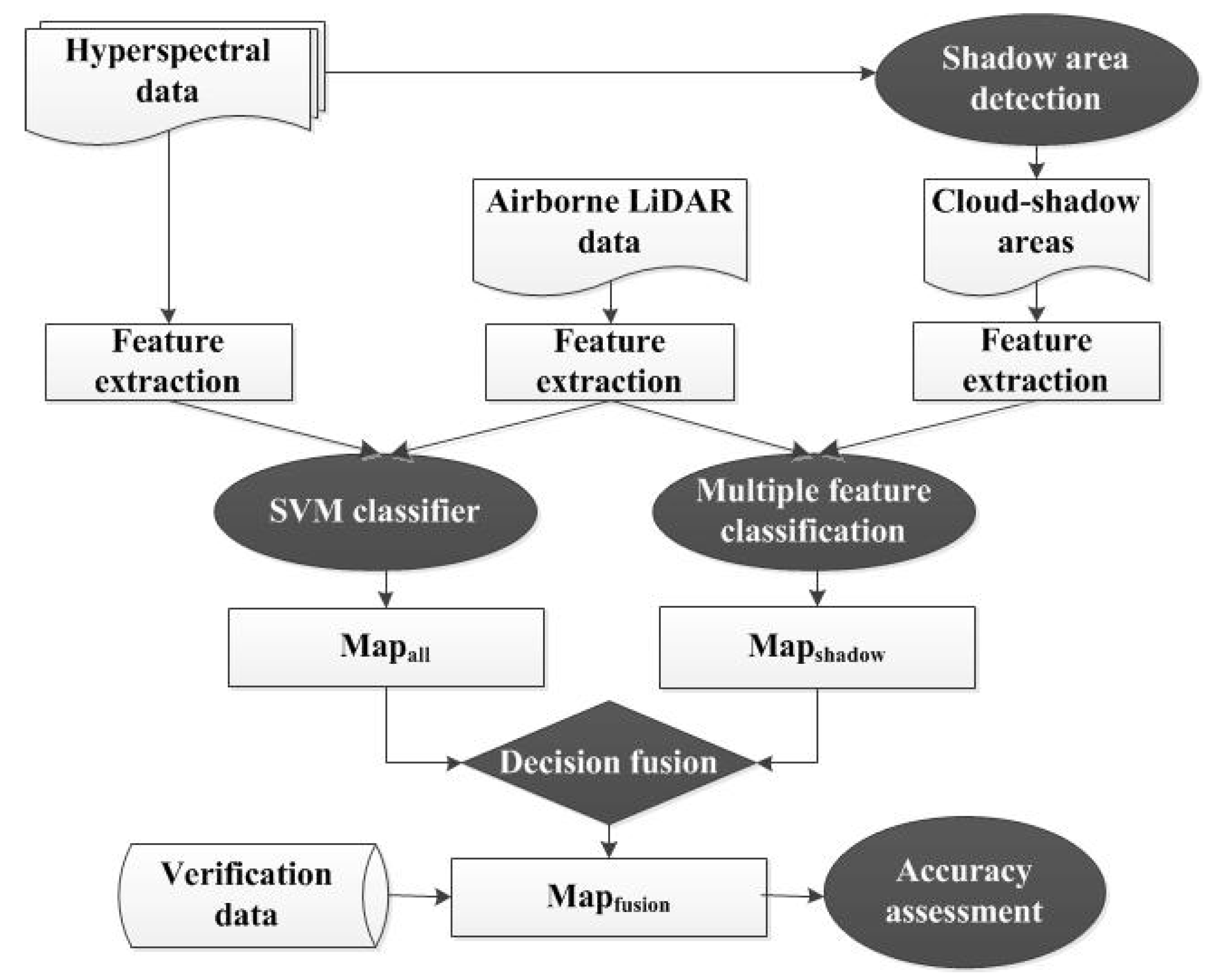
The methodology flowchart consists of six major parts: (1) data preprocessing; (2) cloud shadow extraction; (3) extraction of urban objects from cloud shadow areas using a multi-scale object-based classifier; (4) extraction of urban objects from the whole study area using a pixel-based SVM classifier; (5) decision fusion of the classification results of shadow areas and the whole study area; (6) accuracy assessment for evaluating the performance of the proposed method.
3.1. Data Preprocessing
The LiDAR point clouds were processed into four raster datasets: a digital surface model (DSM), a digital elevation model (DEM), a normalized digital surface model (nDSM), and intensity imagery. The detailed steps are as follows: (1) Terrasolid software was used to filter the raw point cloud data into ground and non-ground points. (2) Inverse distance weighted interpolation (IDW) was used to interpolate ground points to the DEM. (3) The first returns of the LiDAR point cloud data were interpolated to create the DSM. (4) The nDSM was generated by subtracting the DEM from the DSM. Finally, the intensity values of the LiDAR point cloud data were interpolated by IDW in ArcGIS 10.2. The spatial resolution of the four raster datasets was 2.5 × 2.5 m.
Since the hyperspectral imagery has 144 narrow spectral bands, and some of these bands are particularly affected by atmospheric effects, atmospheric correction is necessary during the preprocessing of hyperspectral data. In this study, atmospheric correction was applied to the hyperspectral data using the FLAASH model in ENVI 5.1. Then the hyperspectral imagery after atmospheric correction was processed to generate the normalized difference vegetation index (NDVI). In order to avoid band redundancy [45,46,47], the 144 spectral bands of hyperspectral imagery were processed using the minimum noise fraction rotation (MNF) and principal component analysis (PCA) in ENVI 5.1. It has been demonstrated that the textural features derived from the gray-level co-occurrence matrix (GLCM) can significantly improve the classification accuracy of satellite images [48,49]. Therefore, the first band of PCA was used to generate the GLCM for texture analysis.
The first 22 bands of MNF (MNF22), nDSM, intensity, GLCM homogeneity, GLCM dissimilarity, and GLCM entropy were selected for urban land use classification. The pixel size of the above parameters was 2.5 × 2.5 m. Figure 2 shows the flowchart of the whole study.
3.2. Shadow Area Extraction
Usually, shadows refer to areas in which the imaging rays are completely or partially obscured by obstacles. The pixel value of a shadow area is generally lower than that of the surrounding imaged area. The loss of spectral information of ground objects in shadow areas increases the difficulty of classification. To improve the accuracy of urban object extraction in shadow areas, it is necessary to investigate new methods.
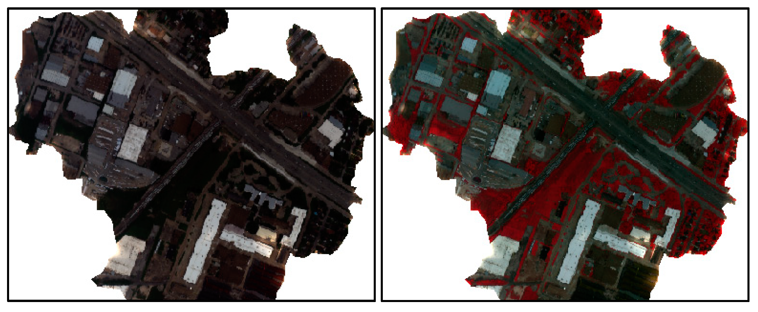
In recent years, many scholars have proposed a variety of shadow detection methods, such as model based and shadow attribute-based detection methods [41,50,51,52,53]. Because the cloud shadow area is very large in our study, and the derivation of the shadow area is not the primary goal of this work, a simple shadow detection method based on area attribute filters was employed [50]. The attribute filters are connected operators. On the basis of a given criterion, attribute filters operate on the connected components that compose an image. Each component of the image is evaluated by the criterion. An arbitrary attribute (e.g., area, volume, etc.) of component C is compared with a given reference value , which is the filter parameter. Taking as an example, if the criterion is verified, the regions remain unaffected; otherwise, they will be set to the gray level of a darker or brighter surrounding region, depending on the transformation used (i.e., thickening or thinning). In this study, by gradually increasing the threshold of the area attribute, progressively more bright objects were filtered out, leaving dark shadow areas. In this study area, two shadow areas were detected: one is large and dark, and the other is small. As we conducted decision fusion of the classification results, the small shadow area was found to be too small to conduct classification individually, let alone decision fusion of the final results. Therefore, only the large main shadow area was chosen for the study. Then, the shadow areas were binarized and used as masks for the subsequent object extraction. M = {} denotes the cloud-shadow mask, with pixel values of = 0 in the cloud-shadow region and = 1 in the shadow-free region. Figure 3 shows the hyperspectral imagery in the shadow area in the true color display and false color display. The vegetation in the shadow area is more apparent in the false color display of the hyperspectral data.
3.3. Extraction of Urban Objects in Cloud Shadow Areas
Information extraction from shadow areas has been a difficult problem in the field of remote sensing. This study mainly utilizes the advantage of airborne LiDAR data and an object-based classification method to improve fusion classification accuracy.
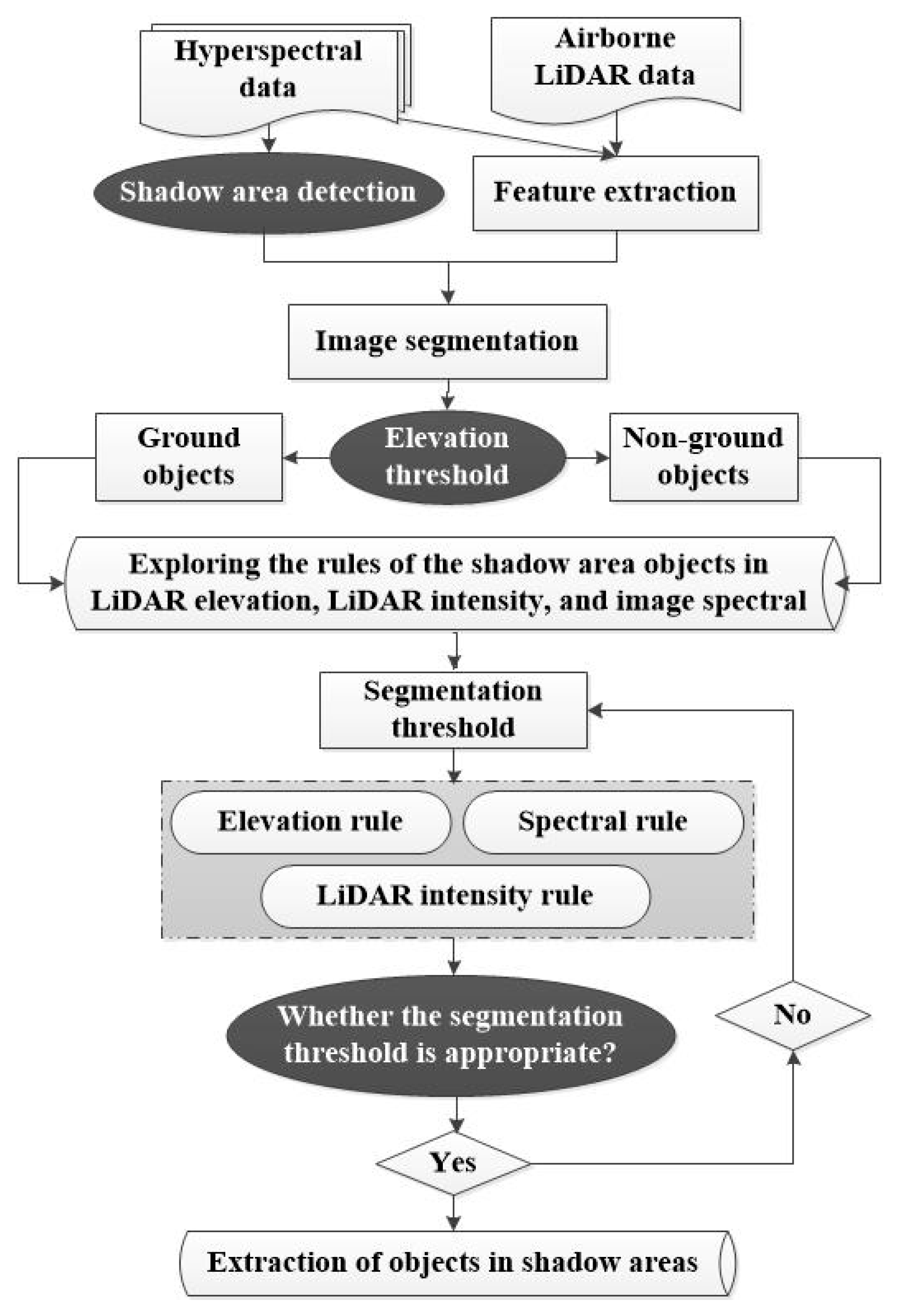
Compared with traditional pixel-based classification methods, object-based classification is an evolving technology that can make full use of spatial, texture, spectral, and other information of the fused data, and it also can reduce the “salt and pepper effect”. Firstly, a multi-resolution segmentation algorithm was used to segment imageries with a certain scale level. Secondly, threshold segmentation classification was conducted to extract urban objects in shadow areas using attributes such as shape, length, and area. As the process is complicated, more detailed information is given in the following sections, which illustrate the images used in the segmentation and the parameters used in the classification. Figure 4 shows a detailed flowchart of the object-based classification in the shadow areas.
3.3.1 Image Segmentation
In object-based classification, segmentation aggregates pixels into objects according to their similarity [44]. As the accuracy of image segmentation significantly influences the classification accuracy [54], the process was performed using the multi-resolution segmentation algorithm (FNEA, fractal net evolution approach) in Trimble eCognition® Developer 9.0. In order to avoid the subjectivity of scale parameter selection and the time-consuming trial-and-error method, the estimation of scale parameter 2 (ESP2) tool was selected to obtain the optimal scale parameter [55,56,57,58]. As an automated tool for segmentation assessment, ESP2 can automatically identify suitable segmentation parameters (SPs) for multi-resolution segmentation on the basis of local variance across scales. The advantages of this strategy are that: (1) different layers have different weights; (2) the attribute (pixel value) and shape of objects are taken into account in the segmentation process; (3) the method is flexible and can make full use of the fused data. After image segmentation, different features were extracted from spectral images to classify the urban objects in the cloud shadows.
3.3.2. Classification Algorithms
(1) Extraction of Buildings
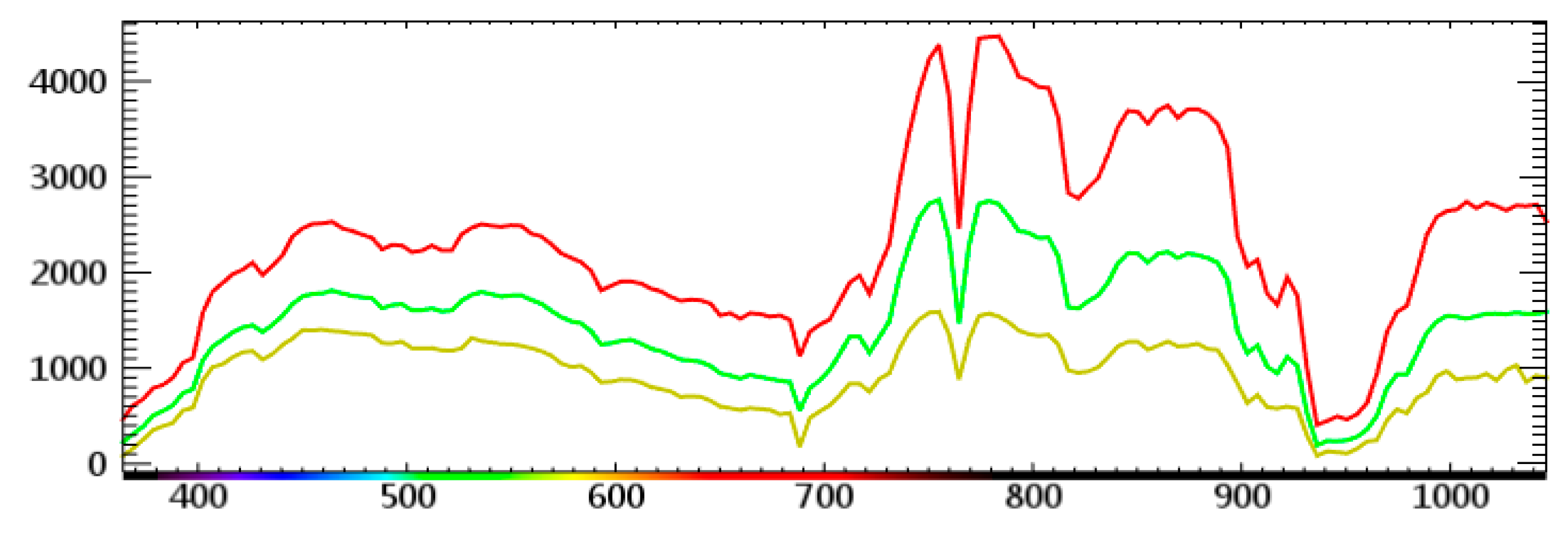
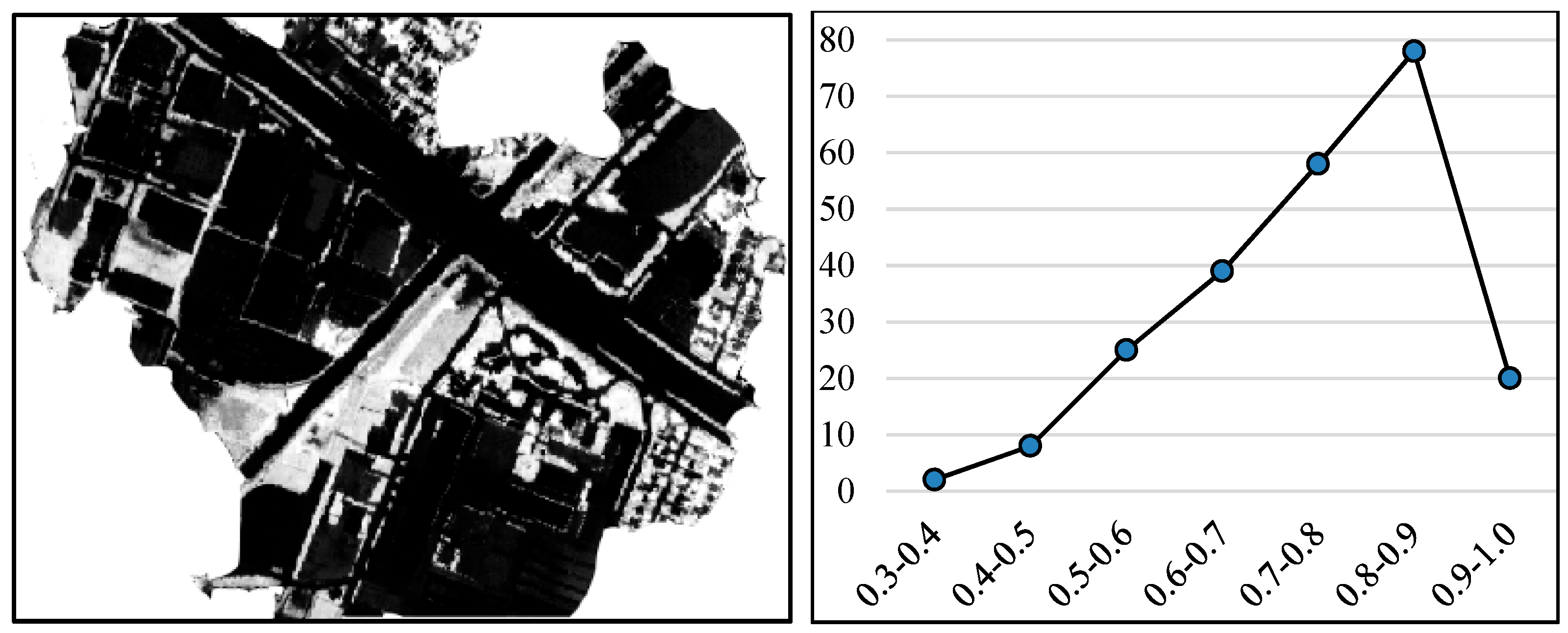
In the hyperspectral imagery, much of the spectral information of shadow areas was lost, so the extraction of objects in shadow areas was difficult. However, some features were still identifiable; for example, vegetation could be identified due to its strong reflectance in the near infrared band. Therefore, we first analyzed the distribution of trees using the normalized difference vegetation index (NDVI), and we then determined the threshold for separating vegetation and non-vegetation on the basis of the NDVI image, which provided a theoretical basis for the subsequent classification. Figure 5 shows the spectral reflectance curves of vegetation in shadow areas. Figure 6 (left) shows the NDVI imagery of the shadow areas. Then, vegetation samples were selected randomly to get their distribution in NDVI imagery, and Figure 6 (right) shows the distribution of vegetation samples in different intervals of NDVI imagery. According to the statistics of sample spectral characteristics, vegetation information in shadow areas was apparent, and the NDVI of vegetation in shadows was greater than 0.3. In addition, the LiDAR height data could assist in the extraction of objects in the shadows. Therefore, the fusion of hyperspectral and LiDAR data could produce better classification results in shadow areas. In order to extract buildings, the nDSM data were first segmented into homogeneous regions using the multi-resolution segmentation method (MRS). The MRS algorithm was run using a shape parameter of 0.4 and a compactness parameter of 0.2. The optimal segmentation scale is 2 according to the calculation of ESP2. Here “scale” means the size of segmented objects, and “shape” and “compactness” are heterogeneity criteria used for merging neighboring objects. Firstly, nDSM was segmented, and then height and NDVI thresholds were used to separate non-ground objects from trees. Secondly, the extracted small objects were merged into large objects. Finally, the geometry parameters (e.g., area, length) were used to separate buildings from other non-ground urban objects. The rules for extracting buildings were set as follows:
- Mean nDSM ≥ 2 m and Mean NDVI ≤ 0.4;
- Merge the extracted segments;
- Length ≤ 450 m and Length/Width ≤ 10;
- Area ≥ 95 m2.
(2) Extraction of trees
In shadow areas, urban objects with height information include buildings, trees, and highways. Therefore, trees were extracted using height information of the nDSM and NDVI. The nDSM data were first segmented into homogeneous regions. Then, the scale, shape, and compact parameters were set as 2, 0.4, and 0.2, respectively. After the nDSM was segmented, the height and NDVI thresholds were used to separate trees from non-ground objects. Then, the extracted small objects were merged into large objects. Finally, the geometry parameters (e.g., area, length) were used to separate trees from other non-ground urban objects. The detailed rules were set as follows:
- Mean NDVI ≥ 0.4 and Mean nDSM ≥ 1 m;
- Merge the extracted segments;
- Area ≥ 5 m2.
(3) Extraction of grass
In shadow areas, the NDVI could be used to separate vegetation and non-vegetation. In addition, the height information of the nDSM could be used to separate trees and grass. Therefore, the rules for the extraction of grass were set as follows:
- Mean NDVI ≥ 0.4 and Mean nDSM < 0.5 m;
- Assign the non-extracted objects to unclassified.
(4) Extraction of highways
Because of the spectral similarity, it is difficult to extract highways, railways, and roads, especially in cloud shadow areas. Here, the unclassified areas were first used as a mask; then, the combined image (Intensity + NDVI + PCA3) was segmented into homogeneous regions using the multi-resolution segmentation method (MRS). The MRS algorithm was run using a shape parameter of 0.1 and a compactness parameter of 0.5. The optimal segmentation scale is 60 according the calculation of ESP2. Finally, the rules were set as follows:
- 10 ≤ Intensity ≤ 71;
- Merge the extracted segments;
- Length ≥ 750 m;
- 2100 m2 < Area < 55,000 m2.
(5) Extraction of railways and roads
Because of the spectral similarity and cloud shadow effect, it is difficult to separate roads from railways. Using the same processing steps as (4) above, the scale, shape, and compact parameters were set as 5, 0.1, and 0.5. Finally, the rules for railway extraction were set as:
- Mean nDSM ≥ 0 m;
- 55 < Intensity < 100;
- Merge the extracted segments;
- 125 m ≤ Length ≤ 500 m;
- 2.2 ≤ compactness ≤ 2.4.
(6) The rules for road extraction were set as:
- Mean nDSM ≥ 0m;
- Mean Intensity ≥ 10;
- 100 m ≤Length ≤ 300 m;
3.4. Extraction of Urban Objects in the Whole Study Area
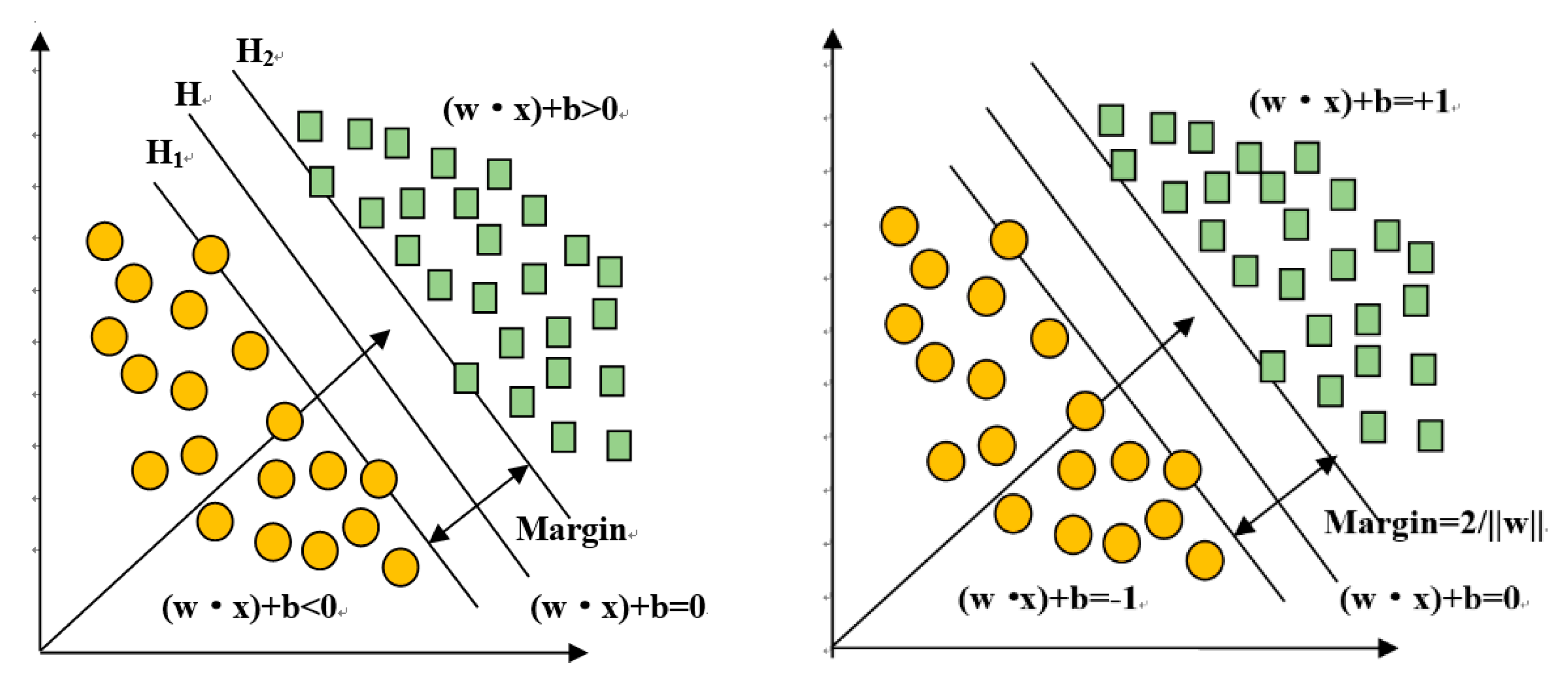
As high-dimensional, multi-source data were used in this study, the traditional parametric classifiers would have been inadequate. The support vector machine (SVM) classifier is a nonparametric algorithm that can produce better classification results with limited training samples [59]. SVM is a supervised machine learning method based on a set of theoretical machine learning algorithms [44,60]. The SVM classification method is dependent on finding a separating hyperplane that provides the best classification between two classes in a multi-dimensional feature space. In an Rn classification situation, the hyperplane can be determined by the following expression. Here, (, ) is a training sample; i = 1, 2, ……n; and w is a vector that is perpendicular to the classification hyperplane.
The hyperplane should maximize the distance between itself and the margin (Figure 7). Here, the margin means the distance from hyperplane to the nearest sample. The larger the margin, the lower the error of classification.
where is the distance from the nearest point to the hyperplane. The function can also be written as:
Finally, the classification plane that can produce the lowest is the optimal hyperplane.
In SVM, the linear and radial basis function (RBF) is frequently used [44,61], and therefore, RBF was used in this study. The input parameters of SVM in the ENVI 5.1 software include “gamma” (γ), “penalty parameter”, “pyramid levels”, and “classification probability threshold”. Since SVM is sensitive to the selection of parameters, cross-validation was used to determine the optimal parameters for the SVM classifier in this study. All of the samples were divided into five parts equally. Each part of the samples was set as an individual validation sample, and the remaining parts were set as training samples. Finally, the average of the five classification accuracies was used as the performance index of the classifier. Using the MATLAB platform, the search range of “penalty parameter” and “gamma” (γ) was set as 0.01–32,768. After cross-validation, the optimal penalty parameter (C) was 1024, the optimal gamma parameter (γ) was 0.045, and the accuracy of cross-validation was 98.70%. In this study, the γ parameter was set to 0.045, the penalty parameter was set to 1024, the pyramid parameter was set to 0, and the classification probability threshold was set to 0.
3.5. Decision Fusion
The definition of image fusion is the combination of two or more different images into a new image using certain algorithms. On the basis of the stage at which fusion happens, image fusion can be divided into three levels: pixel-level, feature-level, and decision-level [62,63]. Decision-level fusion is performed by classifying and identifying each image individually and then getting the optimal decision results. In this study, decision-level fusion was used to make full use of the rich spectral information of hyperspectral data and the advantages of airborne LiDAR data for urban object extraction in shadow areas. As expressed in Equation (4), the final classification map is obtained by the fusion of the two maps:
In the above function, means the final classification map after the decision fusion; Mapall means the classification result obtained by using the SVM classifier and the training samples; Mapshadow means the classification results in shadow areas obtained by using the object-based classifier. The decision fusion process was conducted in ArcGIS 10.2 software. As shown in Table 1, each number (class code) represents a type of urban object: for example, 1 represents grass, and 10 represents tree. The detailed fusion steps are as follows:
- (1)
- Subset with the boundary of the shadow areas;
- (2)
- The class code of the urban objects in defined as trees, buildings, grass, highway, and railway was set to 0, and the class code of the other objects was set to 1;
- (3)
- The raster calculator in ArcGIS 10.2 software was used to multiple (1) by (2);
- (4)
- The class code of the other objects was set to 0;
- (5)
- The raster calculator was used to add (3) and (4).
3.6. Accuracy Assessment
To evaluate the effectiveness of the integration of hyperspectral data and LiDAR data for the classification of urban shadow areas, confusion matrix analysis and the accuracy index (AI) were used [64]. The confusion matrix provides the overall accuracy (OA), the user’s accuracy (UA), and the producer’s accuracy (PA) [30,65]. The confusion matrix is composed of m columns by m rows. By using the confusion matrix, one could determine the number of samples and the number of misclassified samples/missing samples and then analyze the accuracy. The formula for calculating the AI coefficient is shown in Equation (5) [66]:
where OE represents omission error, and CE represents commission error.
In addition, McNemar’s test is conducted to assess the levels of statistically significant difference for all the classification accuracies [44,67,68,69,70]. McNemar’s test is a nonparametric test applied to confusion matrices which have a 2 × 2 dimension. The test is based on chi-square () statistics, which is computed from two error matrices and given as Equation (6) [44].
Here, represents the number of cases that are wrongly classified by classifier 1 but are correctly classified by classifier 2, while represents the number of cases that are correctly classified by classifier 1 but are wrongly classified by classifier 2.
4. Results and Discussion
4.1. Classification Results of Cloud Shadow Areas
The classified image in the shadow area is shown in Figure 8. The results show the capability of the proposed object-based method in hyperspectral and LiDAR data fusion for mapping objects in shadow areas. The proposed object-based classification method can employ the attribute (pixel value) and the shape of objects to make full use of the advantages of the height information from LiDAR data and the spectral information from hyperspectral data. In addition, the proposed method can mitigate the effect of shadows. As can be seen, the nDSM imagery in Figure 9 shows the exact distribution of urban objects with height information, such as buildings and trees, while the hyperspectral imagery in Figure 9 shows the urban objects in shadow areas, especially vegetation in false color display. Therefore, by visual comparison of Figure 8 and Figure 9, the proposed method can classify buildings, trees, and grasses more accurately than the SVM classifier.
4.2. The Decision-fusion Result of the Whole Study Area
The nDSM data are relatively consistent and stable across heterogeneous urban areas, so it is possible to extract objects with height information using the object-based classification method. The decision fusion result of the two classifiers is much better than that of the SVM classifier. The resulting classified images of the whole study area are shown in Figure 10. The decision-fusion results of SVM and OB (object-based classifier) are much better than those of SVM only.
4.3. Accuracy Assessment of the Final Decision Fusion Result
In order to quantify the performance of the proposed method in shadow object extraction, the SVM classification results of the whole study area and the final decision fusion result were compared for accuracy assessment. The accuracy assessments of the classification results are shown in Table 2 and Table 3. Table 2 indicates that, compared with the SVM classifier only, the fused SVM and OB classifier improved the overall accuracy by 5.00% (from 87.30% to 92.30%). The error statistics of the accuracy assessment for 12 classes are listed in Table 3. Since the overall classification results using the kappa-statistic were close, the significance of the results using McNemar’s test statistic was valuated. A total of 14,202 pixels were compared for the accuracy assessment. The non-diagonal cells in the error matrix that represent incorrectly classified pixels after classification with the SVM classifier include 2868 pixels, and the proposed method results include 1473 pixels. In contrast, the diagonal totals that represent the correctly classified values for SVM include 12,412 pixels, and those for the proposed method’s classification include 13,109 pixels. A two-by-two contingency matrix was constructed for the above correctly classified and incorrectly classified pixels and then evaluated using McNemar’s test. The results indicate a chi-square test statistic value of 1304.18, which exceeds the chi-square test critical value of 11.07 (alpha = 0.05) [44]. Thus, the superiority of the proposed method over SVM is accepted. As mentioned earlier, the same training and validation samples were used for all of the classification experiments. Therefore, the proposed method (SVM + OB) significantly improves the classification accuracy, which also means that the proposed object-based classification method can effectively extract urban objects in shadow areas with fused hyperspectral and LiDAR data.
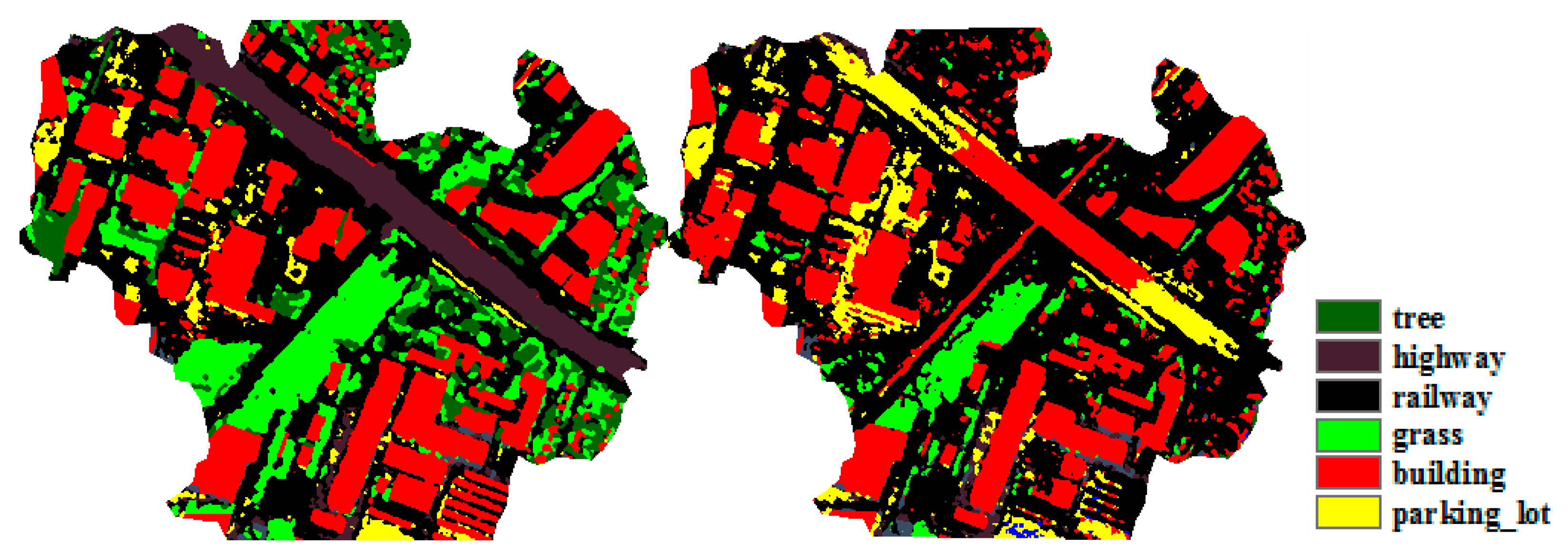
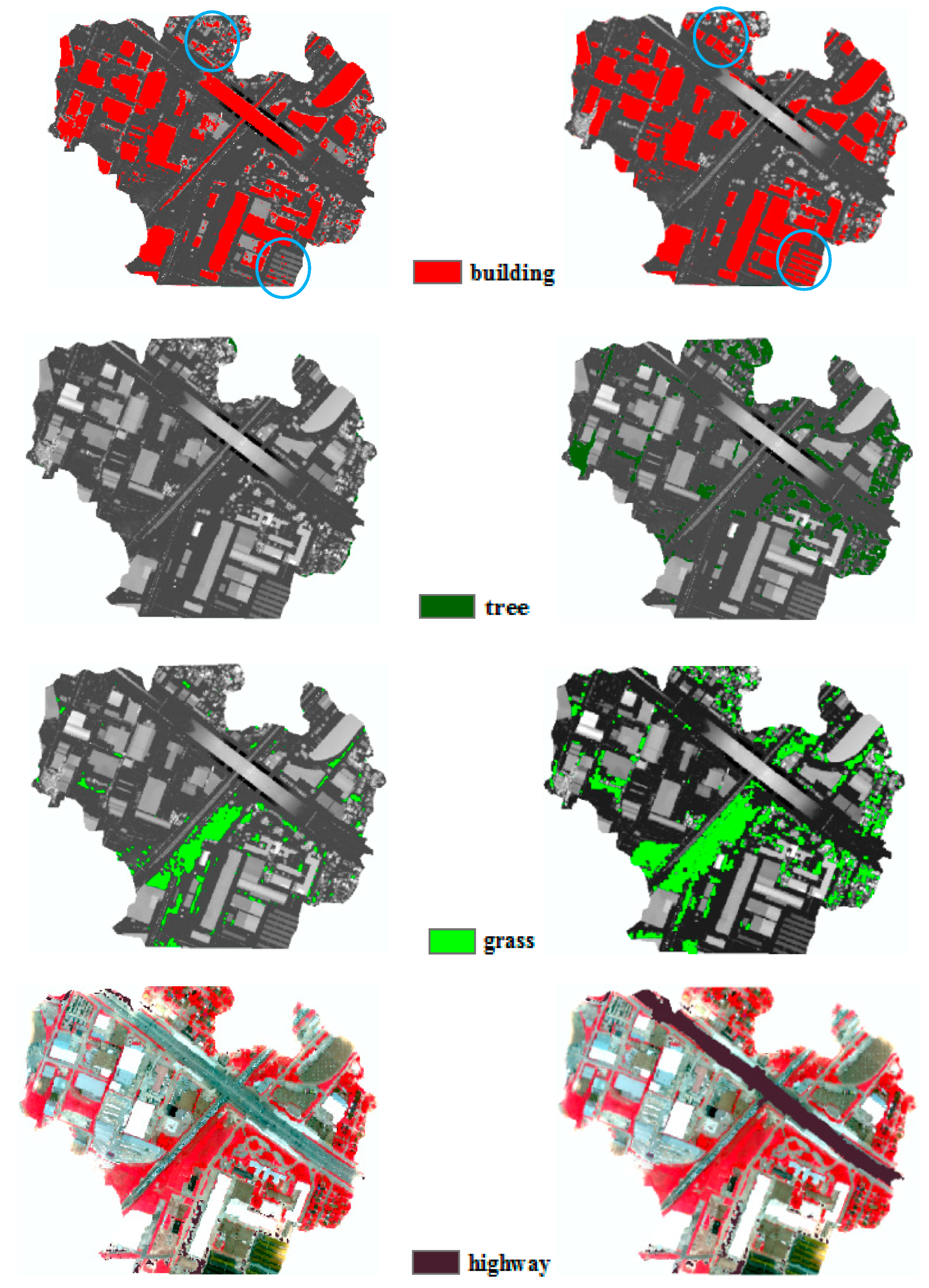
As seen in Table 3, all classes reach a high accuracy except the road, railway, highway, parking_lot, and building classes. Compared with the SVM classifier only, the proposed method improves AI of trees from 88.71% to 93.49%, the AI of highways from 6.76% to 75.72%, the AI of railways from 56.58% to 78.81%, the AI of grass from 93.38% to 98.17%, and the AI of buildings from 63.64% to 86.08%. Using the proposed method to extract shadow area objects improves the overall accuracy from 87.30% to 92.30%, and it also improves the AI of the tree, highway, railway, grass, and building classes by 4.78%, 68.96%, 22.23%, 4.79%, and 22.44%, respectively. In order to better display the performance of object-based classification, the classification results of buildings, trees, grass, and highway using SVM and object-based classifiers are shown in Figure 11. Figure 11 compares the classified urban objects in shadow areas (especially buildings, trees, grass, and highway) resulting from the proposed object-based classification method with those resulting from the traditional pixel-based SVM classifier. As shown in Figure 11 (the blue circle), more buildings (especially residential areas) have been extracted. In addition, the shapes of the buildings are more complete. As shown in Figure 11, it was not possible to extract trees in shadow areas using the traditional pixel-based SVM classifier, whereas the object-based classifier could extract most of the trees in shadow areas. This is mainly because the object-based classifier can make full use of the height information in the nDSM and spectral information of the NDVI imagery, as is the case for the grass. Highways are difficult to extract from hyperspectral imagery, let alone highways in shaded areas. In this study, intensity imagery derived from LiDAR data was also used to extract highways.
4.4. Discussion
In cloud shadow areas, the spectra of the objects are missing, making it difficult to extract urban objects. In this study, two different types of remotely sensed data and a proposed classification method were used to extract objects in cloud shadow areas. The advantages of the method are that: (1) the pixel-based SVM classifier is effective for high -dimensional data classification; (2) the object-based classification method is suitable for classifying nDSM data [71]; (3) decision fusion can fuse different types of data from different sensors, and it is independent of errors in data registration. In this respect, the decision-fusion method is much better than fusion at other levels [72,73]. The object-based classification method uses LiDAR elevation data and shape attributes to separate buildings, trees, and elevated roads. Usually, these are always above ground and part of the highway is aboveground. The elevation information of the nDSM was used to extract the above objects from others. Furthermore, although some spectral information was missing, the NDVI of trees and grass was still obvious and valuable for the separation of vegetation and non-vegetation areas. Therefore, the height information of the nDSM, the spectral information of the NDVI, and the flexible parameters of the object-based classification method were used for the object extraction from cloud shadows. Table 2 shows that the overall accuracy increases from 87.30% to 92.30%. Table 3 shows increased accuracy for buildings, highways, trees, grasses, and railways. Figure 11 also shows the advantage of the object-based classification method in cloud shadow areas using fused hyperspectral-LiDAR data. All of these results indicate the effectiveness of the proposed method.
The results from this study can also be compared with other classifications using fused hyperspectral and LiDAR data. Man et al. [30] fused LiDAR and hyperspectral data in a pixel-level and feature-level fusion strategy, and the overall accuracy of the classification was improved to 94.70%. Because different segmentation methods and spectral band combinations were used, the threshold values are a little different between the two studies. Luo et al. [50] classified the cloud-shadow area with fused hyperspectral and LiDAR data. This study mainly focused on the selection of training data in cloud-shadow areas. The proposed method improves the overall accuracy by 5.00% for the whole study area. However, the scale parameter of the segmentation was unsuitable for all classes. Different urban objects have different heterogeneities. In order to satisfy the best segmentation effect of different urban objects, it is necessary to find the most suitable segmentation scale and obtain different types of image objects. Therefore, the multi-resolution segmentation method was used for the segmentation and the subsequent classification. In summary, the method proposed in this study is valuable for improving the accuracy of urban land cover classification in cloud shadows.
5. Conclusions
The aims of this study are to explore the performance of a proposed method for the extraction of objects in shadow areas using fused hyperspectral and LiDAR data. Although previous studies have evaluated the performance of fused hyperspectral and LiDAR data in urban land use classification, to our knowledge, few studies have attempted to explore the fused hyperspectral and LiDAR data in shadow areas, especially using the object-based hierarchical classification method. This study combined a pixel-based SVM classifier and an object-based hierarchical classifier to extract urban objects in shadow areas using fused hyperspectral and LiDAR data. The following conclusions can be drawn on the basis of these results.
(1) The proposed method yields better accuracy and is confirmed by visual interpretation in urban shadow areas. The decision fusion results of the SVM and object-based classifiers improve the overall classification accuracy by 5.00% (from 87.30% to 92.30%). The overall accuracy improvement mainly occurs in the extraction of objects in the shadow area. In particular, this was observed for the classes of tree (AI increased from 88.71% to 93.49%), highway (AI increased from 6.76% to 75.72%), railway (AI increased from 56.58% to 78.81%), grass (AI increased from 93.38% to 98.17%), and building (AI increased from 63.64% to 86.08%). This is mainly because of the height information of the LiDAR datasets and the flexibility of the object-based classifier, which was very helpful for the separation of trees and low vegetation, buildings, and roads. Overall, the results from this study suggest that the combination of the pixel-based SVM classifier and object-based classifier with fused hyperspectral and LiDAR data has considerable potential to achieve high classification accuracy in urban land use classification, especially for urban object extraction in shadow areas.
(2) Compared with the pixel-level fusion of hyperspectral and LiDAR data, the decision-level fusion of pixel- and object-based classifications is very effective for urban object extraction in shadow areas. However, the segmentation threshold values and rules used in this study may not be readily applicable to other urban areas using the same remotely sensed data.
(3) In the future, the object-based classifier will be applied to the whole study area, and decision level will be fused with the pixel-based SVM classifier in order to obtain a better result and further evaluate the performance of the proposed method for the whole study area. Furthermore, more classification algorithms and multi-source remote sensing data will also be considered to further improve the classification results of the shadow areas.
Author Contributions
Q.M. conceived and designed the methodology of the study, performed the data analysis and wrote the original draft preparation; P.D. reviewed and edit the draft preparation.
Funding
This research is funded by Natural Science Foundation of Shandong Province (NO. ZR2016DB19) for developing a new method for urban object extraction in shadow areas.
Acknowledgments
The first author would like to thank the Hyperspectral Image Analysis group and the NSF-Funded Center for Airborne Laser Mapping (NCALM) at the University of Houston for providing the data sets used in this study, and the IEEE GRSS Data Fusion Technical Committee for organizing the 2013 Data Fusion Contest.
Conflicts of Interest
The authors declare no conflict of interest. The funding sponsors had no role in the design of the study; in the collection, analyses, or interpretation of data; in the writing of the manuscript, and in the decision to publish the results.
References
- Franke, J.; Roberts, D.A.; Halligan, K.; Menz, G. Hierarchical Multiple Endmember Spectral Mixture Analysis (MESMA) of Hyperspectral Imagery for Urban Environments. Remote Sens. Environ. 2009, 113, 1712–1723. [Google Scholar] [CrossRef]
- Ben-Dor, E.; Levin, N.; Saaroni, H.A. Spectral Based Recognition of The Urban Environment Using the Visible and Near-Infrared Spectral Region (0.4–1.1 µm). A Case Study over Tel-Aviv, Israel. Int. J. Remote Sens. 2001, 22, 2193–2218. [Google Scholar] [CrossRef]
- Herold, M.; Roberts, D.A. Spectral Characteristics of Asphalt Road Aging and Deterioration: Implications for Remote-Sensing Applications. Appl. Opt. 2005, 44, 4327–4334. [Google Scholar] [CrossRef]
- Powell, R.L.; Roberts, D.A.; Dennison, P.E.; Hess, L.L. Sub-Pixel Mapping of Urban Land Cover Using Multiple Endmember Spectral Mixture Analysis: Manaus, Brazil. Remote Sens. Environ. 2007, 106, 253–267. [Google Scholar] [CrossRef]
- Cavalli, R.M.; Fusilli, L.; Pascucci, S.; Pignatti, S.; Santini, F. Hyperspectral Sensor Data Capability for Retrieving Complex Urban Land Cover in Comparison with Multispectral Data: Venice City Case Study (Italy). Sensors 2008, 8, 3299–3320. [Google Scholar] [CrossRef] [PubMed]
- Jensen, J.R.; Cowen, D.C. Remote Sensing of Urban Suburban Infrastructure and Socio-Economic Attributes. Photogramm. Eng. Remote Sens. 1999, 65, 611–622. [Google Scholar]
- Small, C. Estimation of Urban Vegetation Abundance by Spectral Mixture Analysis. Int. J. Remote Sens. 2001, 2, 1305–1334. [Google Scholar] [CrossRef]
- Small, C. High Spatial Resolution Spectral Mixture Analysis of Urban Reflectance. Remote Sens. Environ. 2003, 88, 170–186. [Google Scholar] [CrossRef]
- Small, C. A Global Analysis of Urban Reflectance. Int. J. Remote Sens. 2005, 26, 661–681. [Google Scholar] [CrossRef]
- Chen, Y.; Su, W.; Li, J.; Sun, Z. Hierarchical Object Oriented Classification Using Very High Resolution Imagery and Lidar Data over Urban Areas. Adv. Space Res. 2009, 43, 1101–1110. [Google Scholar] [CrossRef]
- Clapham, W.B., Jr. Continuum-Based Classification of Remotely Sensed Imagery to Describe Urban Sprawl on a Watershed Scale. Remote Sens. Environ. 2003, 86, 322–340. [Google Scholar] [CrossRef]
- Ji, M.; Jensen, J.R. Effectiveness of Sub-Pixel Analysis in Detecting and Quantifying Urban Imperviousness from Landsat Thematic Mapper Imagery. Geocarto Int. 1999, 14, 33–41. [Google Scholar] [CrossRef]
- Ghanbari, Z.; Sahebi, M.R. Improved IHS Algorithm for Fusing High Resolution Satellite Images of Urban Areas. J. Indian Soc. Remote Sens. 2014, 42, 689–699. [Google Scholar] [CrossRef]
- Xu, D.; Ni, G.; Jiang, L.; Shen, Y.; Li, T.; Ge, S.; Shu, X. Exploring for Natural Gas Using Reflectance Spectra of Surface Soils. Adv. Space Res. 2008, 41, 1800–1817. [Google Scholar] [CrossRef]
- Gamba, P.; Houshmand, B. Joint Analysis of SAR, LIDAR and Aerial Imagery for Simultaneous Extraction of Land Cover, DTM and 3D Shape of Buildings. Int. J. Remote Sens. 2002, 23, 4439–4450. [Google Scholar] [CrossRef]
- Koetz, B.; Morsdorf, F.; Van Der Linden, S.; Curt, T.; Allgöwer, B. Multi-Source Land Cover Classification for Forest Fire Management Based on Imaging Spectrometry and Lidar Data. For. Ecol. Manag. 2008, 256, 263–271. [Google Scholar] [CrossRef]
- Dalponte, M.; Ørka, H.O.; Ene, L.T.; Gobakken, T.; Næsset, E. Tree Crown Delineation and Tree Species Classification in Boreal Forests Using Hyperspectral and ALS Data. Remote Sens. Environ. 2014, 140, 306–317. [Google Scholar] [CrossRef]
- Ghosh, A.; Fassnacht, F.E.; Joshi, P.K.; Koch, B. A Framework for Mapping Tree Species Combining Hyperspectral and LiDAR data: Role of Selected Classifiers and Sensor across Three Spatial Scales. Int. J. Appl. Earth Obs. 2014, 26, 49–63. [Google Scholar] [CrossRef]
- Zhang, Z.; Kazakova, A.; Moskal, L.; Styers, D. Object-Based Tree Species Classification in Urban Ecosystems Using LiDAR and Hyperspectral Data. Forests 2016, 7, 122. [Google Scholar] [CrossRef]
- Shen, X.; Cao, L. Tree-Species Classification in Subtropical Forests Using Airborne Hyperspectral and LiDAR Data. Remote Sens. 2017, 9, 1180. [Google Scholar] [CrossRef]
- Pontius, J.; Hanavan, R.P.; Hallett, R.A.; Cook, B.D.; Corp, L.A. High Spatial Resolution Spectral Unmixing for Mapping Ash Species Across A Complex Urban Environment. Remote Sens. Environ. 2017, 199, 360–369. [Google Scholar] [CrossRef]
- Man, Q.; Dong, P.; Guo, H. Light Detection and Ranging and Hyperspectral Data for Estimation of Forest Biomass: A review. J. Appl. Remote Sens. 2014, 8, 081598. [Google Scholar] [CrossRef]
- Luo, S.; Wang, C.; Xi, X.; Pan, F.; Peng, D.; Zou, J.; Nie, S.; Qin, H. Fusion of Airborne LiDAR Data and Hyperspectral Imagery for Aboveground and Belowground Forest Biomass Estimation. Ecol. Indic. 2017, 73, 378–387. [Google Scholar] [CrossRef]
- Brovkina, O.; Novotny, J.; Cienciala, E.; Zemek, F.; Russ, R. Mapping Forest Aboveground Biomass Using Airborne Hyperspectral and LiDAR Data in The Mountainous Conditions of Central Europe. Ecol. Eng. 2017, 100, 219–230. [Google Scholar] [CrossRef]
- Wang, J.; Liu, Z.; Yu, H. Mapping Spartina Alterniflora Biomass Using LiDAR and Hyperspectral Data. Remote Sens. 2017, 9, 589. [Google Scholar] [CrossRef]
- Zhang, Y.; Yang, H.L.; Prasad, S.; Pasolli, E.; Jung, J.; Crawford, M. Ensemble Multiple Kernel Active Learning for Classification of Multisource Remote Sensing Data. IEEE J. Sel. Top. Appl. Earth Obs. Remote Sens. 2017, 8, 845–858. [Google Scholar] [CrossRef]
- Zhang, M.; Ghamisi, P.; Li, W. Classification of Hyperspectral and LIDAR Data Using Extinction Profiles with Feature Fusion. Remote Sens. Lett. 2017, 8, 957–966. [Google Scholar] [CrossRef]
- Forzieri, G.; Tanteri, L.; Moser, G.; Catani, F. Mapping Natural and Urban Environments using Airborne Multi-sensor ADS40-MIVIS-LiDAR Synergies. Int. J. Appl. Earth Obs. 2013, 23, 313–323. [Google Scholar] [CrossRef]
- Wang, H.; Glennie, C. Fusion of Waveform LiDAR Data and Hyperspectral Imagery for Land Cover Classification. ISPRS J. Photogramm. 2015, 108, 1–11. [Google Scholar] [CrossRef]
- Man, Q.; Dong, P.; Guo, H. Pixel- and Feature-level Fusion of Hyperspectral and LiDAR Data for Urban Land-use Classification. Int. J. Remote Sens. 2015, 36, 1618–1644. [Google Scholar] [CrossRef]
- Luo, S.; Wang, C.; Xi, X.; Zeng, H.; Li, D.; Xia, S.; Wang, P. Fusion of Airborne Discrete-Return LiDAR and Hyperspectral Data for Land Cover Classification. Remote Sens. 2015, 8, 3. [Google Scholar] [CrossRef]
- Ghamisi, P.; Wu, D.; Cavallaro, G.; Benediktsson, J.A.; Phinn, S.; Falco, N. An Advanced Classifier for The Joint Use of LiDAR and Hyperspectral data: Case Study in Queensland, Australia. In Proceedings of the 2015 IEEE International Geoscience and Remote Sensing Symposium (IGARSS), Milan, Italy, 26–31 July 2015; pp. 2354–2357. [Google Scholar]
- Abbasi, B.; Arefi, H.; Bigdeli, B.; Motagh, M.; Roessner, S. Fusion of Hyperspectral and LiDAR Data Based on Dimension Reduction and Maximum Likelihood. ISPRS Arch. 2015, 40, 569. [Google Scholar] [CrossRef]
- Bigdeli, B.; Samadzadegan, F.; Reinartz, P. A Decision Fusion Method Based on Multiple Support Vector Machine System for Fusion of Hyperspectral and LIDAR Data. IJIDF 2014, 5, 196–209. [Google Scholar] [CrossRef]
- Samadzadegan, F. Feature Grouping-based Multiple Fuzzy Classifier System for Fusion of Hyperspectral and LIDAR Data. J. Appl. Remote Sens. 2014, 8, 083509. [Google Scholar]
- Zhong, Y.; Cao, Q.; Zhao, J.; Ma, A.; Zhao, B.; Zhang, L. Optimal Decision Fusion for Urban Land-Use/Land-Cover Classification Based on Adaptive Differential Evolution Using Hyperspectral and LiDAR Data. Remote Sens. 2017, 9, 868. [Google Scholar] [CrossRef]
- Licciardi, G.; Pacifici, F.; Tuia, D.; Prasad, S.; West, T.; Giacco, F.; Thiel, C.; Inglada, J.; Christophe, E.; Chanussot, J.; et al. Decision Fusion for the Classification of Hyperspectral Data: Outcome of the 2008 GRS-S Data Fusion Contest. IEEE Trans. Geosci. Remote Sens. 2009, 47, 3857–3865. [Google Scholar] [CrossRef] [Green Version]
- Yoon, J.S.; Shin, J.I.; Lee, K.S. Land Cover Characteristics of Airborne LiDAR Intensity Data: A Case Study. IEEE Geosci. Remote Sens. 2008, 5, 801–805. [Google Scholar] [CrossRef]
- Rasti, B.; Ghamisi, P.; Plaza, J.; Plaza, A. Fusion of Hyperspectral and LiDAR Data Using Sparse and Low-Rank Component Analysis. IEEE Trans. Geosci. Remote Sens. 2017, 55, 6354–6365. [Google Scholar] [CrossRef]
- Bigdeli, B.; Samadzadegan, F.; Reinartz, P. Fusion of Hyperspectral and LIDAR Data Using Decision Template-based Fuzzy Multiple Classifier System. Int. J. Appl. Earth Obs. 2015, 38, 309–320. [Google Scholar] [CrossRef]
- Liu, W.; Yamazaki, F. Object-based Shadow Extraction and Correction of High-resolution Optical Satellite Images. IEEE J. Sel. Top. Appl. Earth Obs. Remote Sens. 2012, 5, 1296–1302. [Google Scholar] [CrossRef]
- Bhaskaran, S.; Paramananda, S.; Ramnarayan, M. Per-Pixel and Object-Oriented Classification Methods for Mapping Urban Features Using IKONOS Satellite Data. Appl. Geogr. 2010, 30, 650–665. [Google Scholar] [CrossRef]
- Debes, C.; Merentitis, A.; Heremans, R.; Hahn, J.; Frangiadakis, N.; Kasteren, T.; Liao, W.; Bellens, R.; Pižurica, A.; Gautama, S.; et al. Hyperspectral and LiDAR Data Fusion: Outcome of the 2013 GRSS Data Fusion Contest. IEEE J. Sel. Top. Appl. Earth Obs. Remote Sens. 2014, 7, 2405–2418. [Google Scholar] [CrossRef]
- Petropoulos, G.P.; Kalaitzidis, C.; Prasad Vadrevu, K. Support Vector Machines and Object-Based Classification for Obtaining Land-Use/Cover Cartography from Hyperion Hyperspectral Imagery. Comput. Geosci. 2012, 41, 99–107. [Google Scholar] [CrossRef]
- Pengra, B.W.; Johnston, C.A.; Loveland, T.R. Mapping an Invasive Plant, Phragmites Australis, in Coastal Wetlands Using the EO-1 Hyperion Hyperspectral Sensor. Remote Sens. Environ. 2007, 108, 74–81. [Google Scholar] [CrossRef]
- Binal, C.; Krishnayya, N.S.R. Classification of Tropical Trees Growing in a Sanctuary Using Hyperion (EO-1) and SAM Algorithm. Curr. Sci. 2009, 96, 1601–1607. [Google Scholar]
- Pignatti, S.R.M.; Cavalli, R.M.; Cuomo, V.; Fusilli, L.; Pascucci, S.; Poscolieri, M.; Santini, F. Evaluating Hyperion Capability for Land Cover Mapping in a Fragmented Ecosystem: Pollino National Park, Italy. Remote Sens. Environ. 2009, 113, 622–634. [Google Scholar] [CrossRef]
- Gianinetto, M.; Rusmini, M.; Candiani, G.; Dalla Via, G.; Frassy, F.; Maianti, P.; Marchesi, A.; Rota Nodari, F.; Dini, L. Hierarchical Classification of Complex Landscape with VHR Pan-sharpened Satellite Data and OBIA Techniques. Eur. J. Remote Sens. 2014, 47, 229–250. [Google Scholar] [CrossRef]
- Aguilar, M.A.; Saldaña, M.M.; Aguilar, F.J. GeoEye-1 and WorldView-2 Pan-sharpened Imagery for Object-based Classification in Urban Environments. Int. J. Remote Sens. 2013, 34, 2583–2606. [Google Scholar] [CrossRef]
- Luo, R.; Liao, W.; Zhang, H.; Zhang, L.; Scheunders, P.; Pi, Y.; Philips, W. Fusion of Hyperspectral and LiDAR Data for Classification of Cloud-Shadow Mixed Remote Sensed Scene. IEEE J. Sel. Top. Appl. Earth Obs. Remote Sens. 2017, 10, 3768–3781. [Google Scholar] [CrossRef]
- Wang, Q.; Yan, L.; Yuan, Q.; Ma, Z. An Automatic Shadow Detection Method for VHR Remote Sensing Orthoimagery. Remote Sens. 2017, 9, 469. [Google Scholar] [CrossRef]
- Alireza, S.; Mehdi, M.; Mohammad, V.Z. Shadow-Based Hierarchical Matching for the Automatic Registration of Airborne LiDAR Data and Space Imagery. Remote Sens. 2016, 8, 466. [Google Scholar] [Green Version]
- Shahtahmassebi, A.R.; Yang, N.; Wang, K.; Moore, N.; Shen, Z. Review of Shadow Detection and De-shadowing Methods in Remote Sensing. Chin. Geogr. Sci. 2013, 23, 403–420. [Google Scholar] [CrossRef]
- Kiani, K.; Mojaradi, B.; Esmaeily, A.; Salehi, B. Urban Area Object-based Classification by Fusion of Hyperspectral and LiDAR Data. In Proceedings of the 2014 IEEE Geoscience and Remote Sensing Symposium, Quebec City, QC, Canada, 13–18 July 2014; pp. 4832–4835. [Google Scholar]
- Drǎguţ, L.; Tiede, D.; Levick, S.R. ESP: A Tool to Estimate Scale Parameter for Multiresolution Image Segmentation of Remotely Sensed Data. Int. J. Geogr. Inf. Sci. 2010, 24, 859–871. [Google Scholar] [CrossRef]
- Belgiu, M.; Csillik, O. Sentinel-2 Cropland Mapping Using Pixel-based and Object-based Time-Weighted Dynamic Time Warping Analysis. Remote Sens. Environ. 2017, 204, 509–523. [Google Scholar] [CrossRef]
- Drăguţ, L.; Csillik, O.; Eisank, C.; Tiede, D. Automated Parameterisation for Multi-scale Image Segmentation on Multiple Layers. ISPRS J. Photogramm. Remote Sens. 2014, 88, 119–127. [Google Scholar] [CrossRef]
- Novelli, A.; Aguilar, M.; Aguilar, F.; Nemmaoui, A.; Tarantino, E. AssesSeg-A Command Line Tool to Quantify Image Segmentation Quality: A Test Carried Out in Southern Spain from Satellite Imagery. Remote Sens. 2017, 9, 40. [Google Scholar] [CrossRef]
- Karimi, Y.; Prasher, S.O.; Patel, R.M.; Kim, S.H. Application of Support Vector Machine Technology for Weed and Nitrogen Stress Detection in Corn. Comput. Electron. Agric. 2006, 51, 99–109. [Google Scholar] [CrossRef]
- Fauvel, M.; Benediktsson, J.A.; Chanussot, J.; Sveinsson, J.R. Spectral and Spatial Classification of Hyperspectral Data Using SVMs and Morphological Profiles. IEEE Trans. Geosci. Remote Sens. 2008, 46, 3804–3814. [Google Scholar] [CrossRef] [Green Version]
- Petropoulos, G.P.; Arvanitis, K.; Sigrimis, N. Hyperion Hyperspectral Imagery Analysis Combined with Machine Learning Classifiers for Land Use/Cover Mapping. Expert Syst. Appl. 2012, 39, 3800–3809. [Google Scholar] [CrossRef]
- Pohl, C.; Van Genderen, J.L. Review Article Multisensor Image Fusion in Remote Sensing: Concepts, Methods and Applications. Int. J. Remote Sens. 1998, 19, 823–854. [Google Scholar] [CrossRef]
- Geerling, G.W.; Labrador-Garcia, M.; Clevers, J.; Ragas, A.M.J.; Smits, A.J.M. Classification of Floodplain Vegetation by Data Fusion of Spectral (CASI) and LiDAR Data. Int. J. Remote Sens. 2007, 28, 4263–4284. [Google Scholar] [CrossRef]
- Antonarakis, A.S.; Richards, K.S.; Brasington, J. Object-Based Land Cover Classification Using Airborne LiDAR. Remote Sens. Environ. 2008, 112, 2988–2998. [Google Scholar] [CrossRef]
- Congalton, R.G. A Review of Assessing the Accuracy of Classifications of Remotely Sensed Data. Remote Sens. Environ. 1991, 37, 35–46. [Google Scholar] [CrossRef]
- Pouliot, D.A.; King, D.J.; Bell, F.W.; Pitt, D.G. Automated Tree Crown Detection and Delineation in High-Resolution Digital Camera Imagery of Coniferous Forest Regeneration. Remote Sens. Environ. 2002, 82, 322–334. [Google Scholar] [CrossRef]
- Bradley, J.V. Distribution-Free Statistical Test; Prentice-Hall: EnglewoodCliffs, NJ, USA, 1968. [Google Scholar]
- Agresti, A. An Introduction to Categorical Data Analysis; Wiley: New York, NY, USA, 1996. [Google Scholar]
- Onojeghuoa, A.O.; Onojeghuo, A.R. Object-based Habitat Mapping Using Very High Spatial Resolution Multispectral and Hyperspectral Imagery with LiDAR Data. Int. J. Appl. Earth Obs. 2017, 59, 79–91. [Google Scholar] [CrossRef]
- Shao, G.; Pauli, B.P.; Haulton, G.S.; Zollner, P.A.; Shao, G. Mapping Hardwood Forests Through a Two-stage Unsupervised Classification by Integrating Landsat Thematic Mapper and Forest Inventory Data. J. Appl. Remote Sens. 2014, 8, 083546. [Google Scholar] [CrossRef]
- Zhou, W. An Object-Based Approach for Urban Land Cover Classification: Integrating LiDAR Height and Intensity Data. IEEE Geosci. Remote Sens. 2013, 10, 928–931. [Google Scholar] [CrossRef]
- Du, P.; Liu, S.; Xia, J.; Zhao, Y. Information Fusion Techniques for Change Detection from Multi-temporal Remote Sensing Images. Inform. Fusion 2013, 14, 19–27. [Google Scholar] [CrossRef]
- Dong, J.; Zhuang, D.; Huang, Y.; Fu, J. Advances in Multi-sensor Data Fusion: Algorithms and Applications. J. Sens. 2009, 9, 7771–7784. [Google Scholar] [CrossRef]
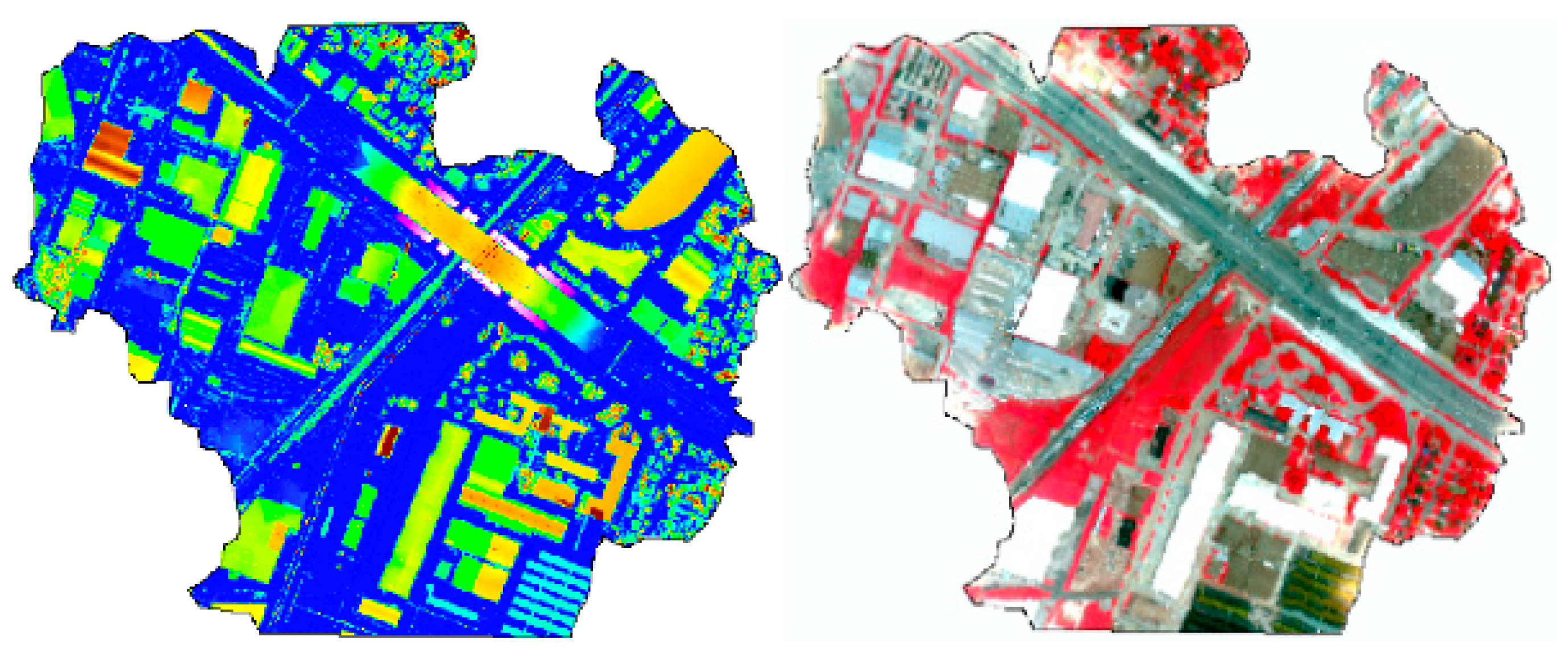
Figure 1.
False color composite of hyperspectral imagery (top) and the normalized digital surface model (nDSM) derived from LiDAR data (bottom).
Figure 1.
False color composite of hyperspectral imagery (top) and the normalized digital surface model (nDSM) derived from LiDAR data (bottom).

Figure 2.
Flowchart of the proposed method.

Figure 3.
Hyperspectral imagery in cloud-shadow areas, true color display (left) and false color display (right).
Figure 3.
Hyperspectral imagery in cloud-shadow areas, true color display (left) and false color display (right).

Figure 4.
The flowchart of urban object extraction from shadow areas with the fusion of airborne light detection and ranging (LiDAR) and hyperspectral data.
Figure 4.
The flowchart of urban object extraction from shadow areas with the fusion of airborne light detection and ranging (LiDAR) and hyperspectral data.

Figure 5.
Spectral curve of vegetation in shadow areas. Here, red/green/yellow lines represent max/mean/min values of hyperspectral data, respectively. The longitudinal axis represents radiance, and the transverse axis represents wavelength (nm).
Figure 5.
Spectral curve of vegetation in shadow areas. Here, red/green/yellow lines represent max/mean/min values of hyperspectral data, respectively. The longitudinal axis represents radiance, and the transverse axis represents wavelength (nm).

Figure 6.
Normalized difference vegetation index (NDVI) imagery of the shadow area (left) and the distribution of vegetation samples in different intervals of the NDVI (right). Here, longitudinal and transverse axes represent the number of samples and NDVI, respectively.
Figure 6.
Normalized difference vegetation index (NDVI) imagery of the shadow area (left) and the distribution of vegetation samples in different intervals of the NDVI (right). Here, longitudinal and transverse axes represent the number of samples and NDVI, respectively.

Figure 7.
Optimal classified hyperplane (left) and Normalization Optimal classified hyperplane (right).
Figure 7.
Optimal classified hyperplane (left) and Normalization Optimal classified hyperplane (right).

Figure 8.
Classified maps in the shadow area obtained from object-based classification (left) and the traditional pixel-based support vector machine (SVM) classifier (right).
Figure 8.
Classified maps in the shadow area obtained from object-based classification (left) and the traditional pixel-based support vector machine (SVM) classifier (right).

Figure 9.
The nDSM imagery of the cloud shadow area (left) and the hyperspectral data of the cloud shadow area (right).
Figure 9.
The nDSM imagery of the cloud shadow area (left) and the hyperspectral data of the cloud shadow area (right).

Figure 10.
The traditional pixel-based SVM classified map of the whole study area (top) and the final decision fusion classification map (bottom).
Figure 10.
The traditional pixel-based SVM classified map of the whole study area (top) and the final decision fusion classification map (bottom).

Figure 11.
A comparison of the classified results in the shadow area between the traditional pixel-based SVM classifier (left) and the proposed object-based classification method (right).
Figure 11.
A comparison of the classified results in the shadow area between the traditional pixel-based SVM classifier (left) and the proposed object-based classification method (right).


Table 1.
Details of training and validation samples used for classification.
| Sample No. | Class | Training | Validation | ||
|---|---|---|---|---|---|
| No. of Polygons | No. of Pixels | No. of Polygons | No. of Pixels | ||
| 1 | grass | 27 | 352 | 50 | 1731 |
| 2 | grass_synthetic | 2 | 192 | 1 | 505 |
| 3 | road | 14 | 140 | 35 | 891 |
| 4 | soil | 13 | 186 | 20 | 1056 |
| 5 | railway | 1 | 31 | 7 | 293 |
| 6 | parking_lot | 26 | 376 | 33 | 1306 |
| 7 | tennis_ court | 2 | 181 | 3 | 247 |
| 8 | running_track | 2 | 187 | 5 | 473 |
| 9 | water | 7 | 182 | 7 | 143 |
| 10 | trees | 15 | 173 | 49 | 880 |
| 11 | building | 51 | 341 | 100 | 1289 |
| 12 | highway | 5 | 109 | 7 | 299 |
Table 2.
Comparison of overall accuracy of SVM and SVM + OB (object-based) decision-fusion results using fused hyperspectral and LiDAR data. OA means overall accuracy.
Table 2.
Comparison of overall accuracy of SVM and SVM + OB (object-based) decision-fusion results using fused hyperspectral and LiDAR data. OA means overall accuracy.
| Data | SVM | SVM + OB | ||
|---|---|---|---|---|
| OA (%) | Kappa Coefficient | OA (%) | Kappa Coefficient | |
| hyperspectral + LiDAR | 87.30% | 0.85 | 92.30% | 0.91 |
Table 3.
Classification results at the class level using SVM and SVM + OB classifiers. PA, producer’s accuracy; UA, user’s accuracy; AI, accuracy index.
Table 3.
Classification results at the class level using SVM and SVM + OB classifiers. PA, producer’s accuracy; UA, user’s accuracy; AI, accuracy index.
| Classes | SVM | SVM + OB | ||||
|---|---|---|---|---|---|---|
| PA (%) | UA (%) | AI (%) | PA (%) | UA (%) | AI (%) | |
| grass_synthetic | 98.94 | 100.00 | 98.93 | 98.94 | 100.00 | 98.93 |
| tree | 90.61 | 99.09 | 88.71 | 97.12 | 96.58 | 93.49 |
| soil | 100.00 | 98.23 | 98.20 | 100.00 | 98.23 | 98.20 |
| water | 98.60 | 100.00 | 98.58 | 98.60 | 100.00 | 98.58 |
| road | 71.42 | 88.85 | 47.42 | 71.42 | 88.85 | 47.42 |
| highway | 57.58 | 83.63 | 6.76 | 89.54 | 88.82 | 75.72 |
| railway | 96.85 | 71.35 | 56.58 | 96.02 | 85.44 | 78.81 |
| tennis_court | 100.00 | 92.31 | 91.66 | 100.00 | 92.31 | 91.66 |
| running_track | 98.77 | 99.65 | 98.40 | 98.77 | 99.65 | 98.40 |
| grass | 94.18 | 99.57 | 93.38 | 98.98 | 99.22 | 98.17 |
| building | 88.95 | 80.69 | 63.64 | 94.50 | 92.85 | 86.08 |
| parking_lot | 81.02 | 75.57 | 44.25 | 81.02 | 79.75 | 51.18 |
© 2019 by the authors. Licensee MDPI, Basel, Switzerland. This article is an open access article distributed under the terms and conditions of the Creative Commons Attribution (CC BY) license (http://creativecommons.org/licenses/by/4.0/).
Share and Cite
MDPI and ACS Style
Man, Q.; Dong, P. Extraction of Urban Objects in Cloud Shadows on the basis of Fusion of Airborne LiDAR and Hyperspectral Data. Remote Sens. 2019, 11, 713. https://0-doi-org.brum.beds.ac.uk/10.3390/rs11060713
AMA Style
Man Q, Dong P. Extraction of Urban Objects in Cloud Shadows on the basis of Fusion of Airborne LiDAR and Hyperspectral Data. Remote Sensing. 2019; 11(6):713. https://0-doi-org.brum.beds.ac.uk/10.3390/rs11060713
Chicago/Turabian StyleMan, Qixia, and Pinliang Dong. 2019. "Extraction of Urban Objects in Cloud Shadows on the basis of Fusion of Airborne LiDAR and Hyperspectral Data" Remote Sensing 11, no. 6: 713. https://0-doi-org.brum.beds.ac.uk/10.3390/rs11060713
Note that from the first issue of 2016, this journal uses article numbers instead of page numbers. See further details here.