A Non-Reference Temperature Histogram Method for Determining T_c from Ground-Based Thermal Imagery of Orchard Tree Canopies

Abstract

Obtaining average canopy temperature (T_c) by thresholding canopy pixels from on-ground thermal imagery has historically been undertaken using ‘wet’ and ‘dry’ reference surfaces in the field (reference temperature thresholding). However, this method is extremely time inefficient and can suffer inaccuracies if the surfaces are non-standardised or unable to stabilise with the environment. The research presented in this paper evaluates non-reference techniques to obtain average canopy temperature (T_c) from thermal imagery of avocado trees, both for the shaded side and sunlit side, without the need of reference temperature values. A sample of 510 thermal images (from 130 avocado trees) were acquired with a FLIR B250 handheld thermal imaging camera. Two methods based on temperature histograms were evaluated for removing non-canopy-related pixel information from the analysis, enabling T_c to be determined. These approaches included: 1) Histogram gradient thresholding based on temperature intensity changes (HG); and 2) histogram thresholding at one or more standard deviation (SD) above and below the mean. The HG method was found to be more accurate (R² > 0.95) than the SD method in defining canopy pixels and calculating T_c from each thermal image (shaded and sunlit) when compared to the standard reference temperature thresholding method. The results from this study present an alternative non-reference method for determining T_c from ground-based thermal imagery without the need of calibration surfaces. As such, it offers a more efficient and computationally autonomous method that will ultimately support the greater adoption of non-invasive thermal technologies within a precision agricultural system.

1. Introduction

In agriculture, the average canopy temperature (T_c) extracted from digital thermal imagery (TI) is increasingly being used to non-destructively quantify plant water status and therefore help in the more efficient irrigation of crops [1,2,3,4,5]. In order to achieve this, thermal images have to be pre-processed to exclude non-leaf pixels (tree stems, shiny leaves, background sky, and other material) depending on the angle of view [6,7].

Currently, specialised image analysis software that often accompanies the thermal cameras, e.g., FLIR QuickReport®, Reporter Pro®, and FLIR ThermaCAM™ Researcher software (FLIR Systems, USA) [7,8], can be used to undertake a limited amount of thermal image pre-processing. However, these software packages generally provide only basic computation functions such as providing mean, maximum, and minimum temperatures from specified regions of interests (ROI) that are typically manually defined by the user for each image [7,9]. Furthermore, these packages provide additional features such as exporting thermal image temperature values (degrees Celsius) into .CSV file formats for a single image at a time. This approach becomes challenging and time consuming when processing large numbers of thermal images (bulk processing), or if the spatial processing requirements vary from image to image, such as when segregating canopy pixels from non-leaf pixels (e.g., background sky). A methodology to sort the canopy pixels in thermal imagery is the use of coincident red, green, and blue (RGB) colour images [10,11]. However, this process does require an RGB image to be acquired at precisely the same time as the thermal image, to account for slight changes in orientation as a result of external factors such as wind. Both the RGB and thermal images have to be accurately aligned spatially, and an RGB ROI or mask needs to be additionally developed to then be applied to the thermal image. If the mask is not accurate, then the extracted T_c may be influenced by the inclusion of non-canopy-specific and mixed pixels.

Another common method used for differentiating (thresholding) canopy from non-canopy pixels is the use of both ‘wet’ (T_wet) and ‘dry’ (T_dry) temperature values, measured from reference panels included in the thermal image of the plant canopy. These T_wet and T_dry values are assumed to correspond to the temperature of the leaf/canopy with and without the cooling effects of transpiration, respectively [12]. Several methods have been proposed to measure both T_wet and T_dry in situ, and these include: (a) Using energy balance algorithms with ancillary weather variables recorded from a weather station [7], (b) direct measurements of leaf/canopy temperature by an IR thermometer to provide the lowest (T_min) and highest (T_max) temperature points of the canopy [13], and (c) use of ‘wet’ and ‘dry’ calibration panels (reference surfaces) [6]. Of these methods, reference surfaces are the most commonly used to threshold canopy pixels under varying environmental conditions [5,6,8]. Typically, several leaves from the canopy are sprayed with soapy water to act as a wet reference (T_wetRef), whilst other leaves are coated with petroleum jelly to restrict transpiration, thus providing a dry reference (T_dryRef). Both are included in the field of view of each subsequent thermal image of a target plant canopy [7]. The reference surfaces allow T_min and T_max values to be calculated from each canopy image, with pixels outside of this range identified as non-canopy specific. With the removal of non-canopy-related pixel information, T_c can be derived by averaging the remaining pixels (which are associated with the canopy). Although this method has been proven to be accurate, the use of reference panels is time consuming, and therefore not ideal when large sample sets are required. As such, automated non-reference methods offer the advantage of applicability.

Although there have been several attempts to automate the pre-processing of thermal imagery, these methods still require inputs from reference surfaces and/or additional measures of canopy temperature for spatial filtering. Fuentes et al. [7] automated part of the filtering process in MATLAB® 2010b (MathWorks Inc., USA) by incorporating the T_wetRef and T_dryRef values obtained from a handheld FLIR B360 camera. However, this method still required the manual delineation of the reference panels and the extraction of average reference values from each image. A similar semi-automated method was attempted by García-Tejero et al. [14], using the C program. However, this process required the input of T_min and T_max temperatures measured from each canopy before processing each image. Measures of T_wet and T_dry are critical for obtaining T_c, but to achieve complete automation without the need for reference panels or additional point source temperature measures, an alternative technique that is exclusively based on digital thermal image itself is desirable.

The aim of this work is to develop a simple, but robust computational technique to automatically threshold canopy specific pixels from the temperature histograms of thermal imagery and to subsequently derive T_c without the need for physical reference targets. This automated method would significantly increase time efficiencies in the collection of canopy temperature data and support scalability, as well as reduce potential errors associated with non-standardised calibration targets. These outcomes support the increased use of on-ground thermal imagery in agriculture.

2. Materials and Methods

This research was conducted as a component of a larger project reported in Salgadoe et al. [15]. The field site was a commercial avocado orchard (cv. Haas), located near Childers (Bundaberg region), Queensland, Australia (24°51′0″S, 152°21′0″E). Avocado trees were of the same age, but canopy densities varied (closed to opened) as the result of Phytophthora root rot (PRR) disease. Further details of the field study site can be found in Salgadoe et al. [15]. A flow diagram of methodologies carried out in this study is shown in Figure 1.

2.1. Ground Thermal Image Acquisition

2.1.1. Canopies

Thermal images of avocado tree canopies were acquired with a handheld thermal camera (FLIR B250; FLIR^® Systems, USA, 7.5–13 µm, 200 × 150 pixel resolution with a thermal sensitivity: 0.07 °C @ +30 °C / 70 mK, field of view (FOV): 25° x 19°). A total of 510 canopy images were obtained from both sides (shaded and sunlit) of 130 avocado trees.

A camera-to-tree distance of 4 m was maintained for all sampled trees to produce comparable 320 × 240 pixel resolution JPEG images. A camera elevation angle of 45° above the horizontal was adopted to ensure only canopy features with clear sky (no sun disk) were included in the background of each image. Due to the orientation of tree rows (north–south direction) there was a high possibility of including sun disk in the camera view, which could distort the canopy image. This view angle also ensured that tree canopies from adjacent rows behind the selected target trees were not included [15]. All images were acquired during mid-day from 1100 h to 1400 h (AEST) with minimal wind conditions and clear skies, conditions that coincide with the maximum evapotranspiration demand of the canopies [7]. Relative humidity and air temperature at mid-canopy level was measured using a hygrometer throughout the image survey (Analog P2501, GH Zeal Ltd., England).

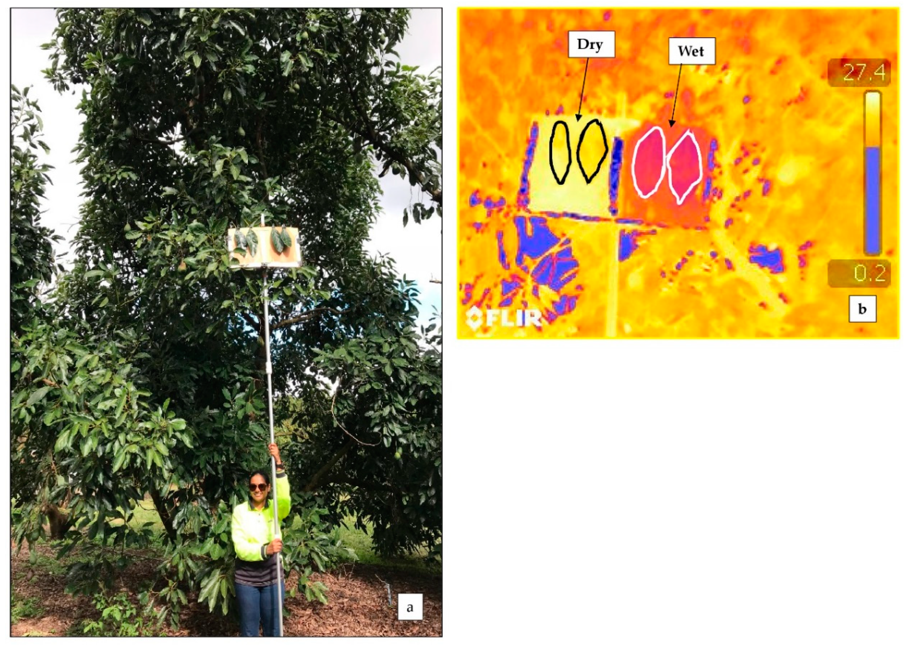
2.1.2. Reference Surfaces

To calibrate and then validate the non-reference methods, thermal images of ‘dry’ and ‘wet’ reference surfaces were acquired during the image survey. These reference surfaces were prepared according to Jones et al. [6] using four mature leaves detached from the canopy. Two leaves serving as ‘dry’ references had a layer of liquid petroleum jelly (Vaseline) applied to both the abaxial and adaxial sides 1 minute before image acquisition. The two ‘wet’ reference leaves had a solution of water and detergent 0.01 % (v/v) applied. These references were then clipped onto a flat panel attached to a steel telescopic pole (>4 m) and positioned beside the tree canopy so as to ensure that they were included in the field of view (FOV) of each respective thermal image (Figure 2a). Precise orientation of tree rows enabled the capture of references on both shaded and sunlit sides of the trees. Thermal images of reference surfaces were only obtained every 3-4 trees, as opposed to every individual tree. The ‘wet’ and ‘dry’ values for those trees that did not have reference surfaces in the FOV were inferred from interpolation of those nearest tree values from either side of them, as outlined below.

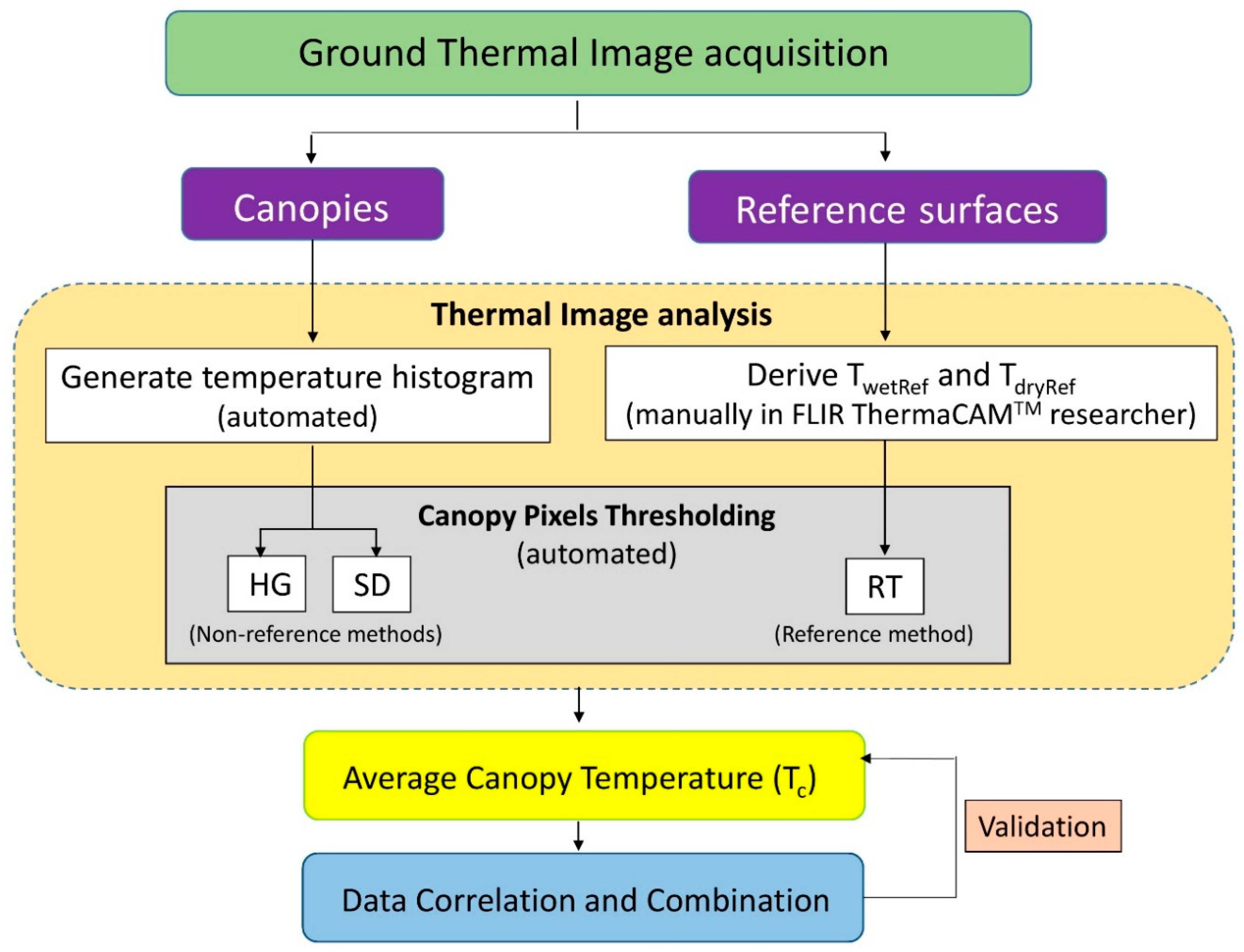
2.2. Thermal Image Analysis

Obtained thermal images of canopies and reference surfaces were analysed separately to derive surface temperatures (degrees Celsius). Canopy thermal images were bulk processed by a custom-coded script [16] to output a temperature data file and construct a temperature histogram for each image. Thermal images of reference surfaces were processed manually by using commercially available software FLIR ThermaCAM^™ researcher (FLIR Systems, USA) to obtain temperatures T_wetRef and T_dryRef for each side of each tree (namely sunlit and shaded) [7].

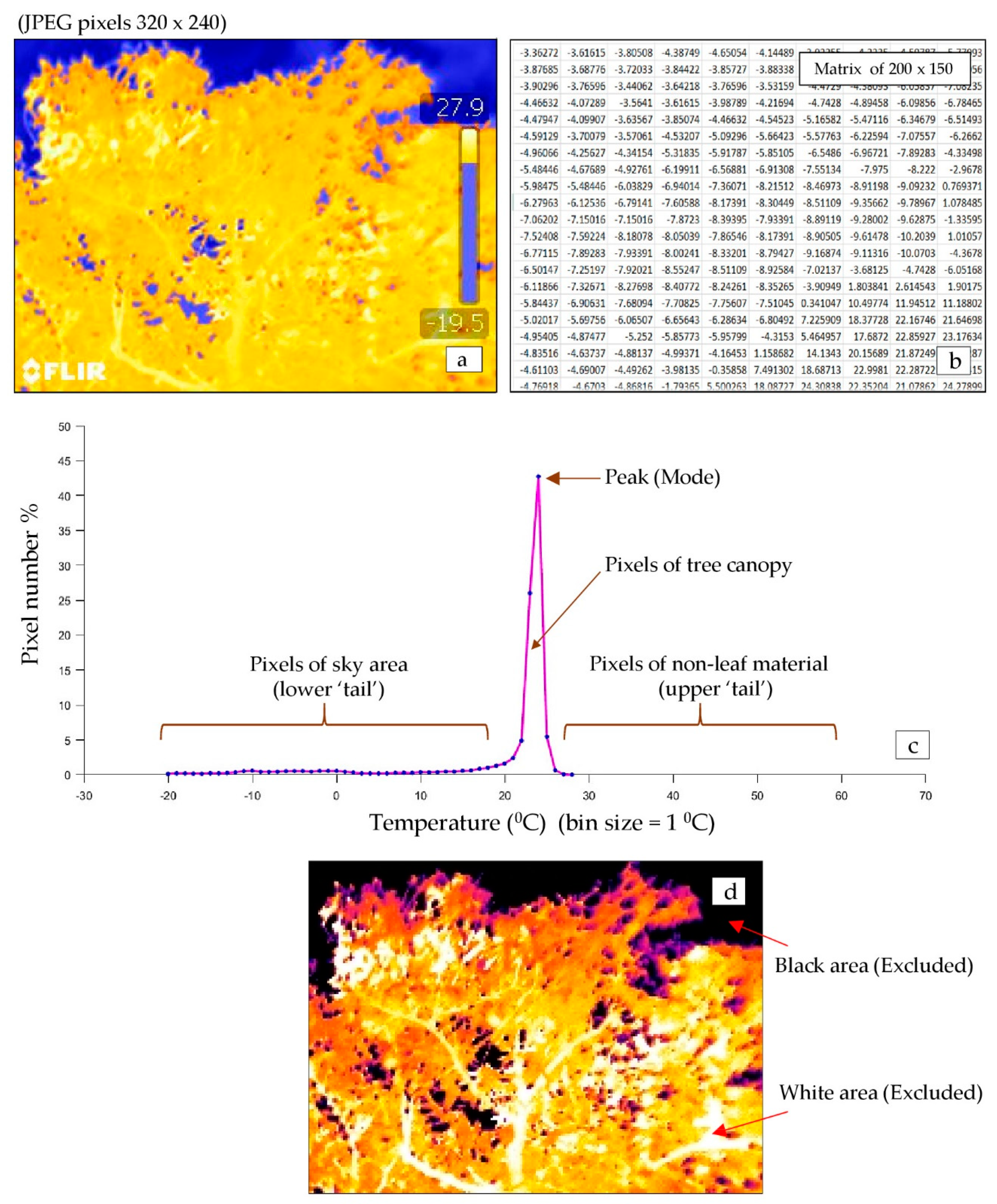
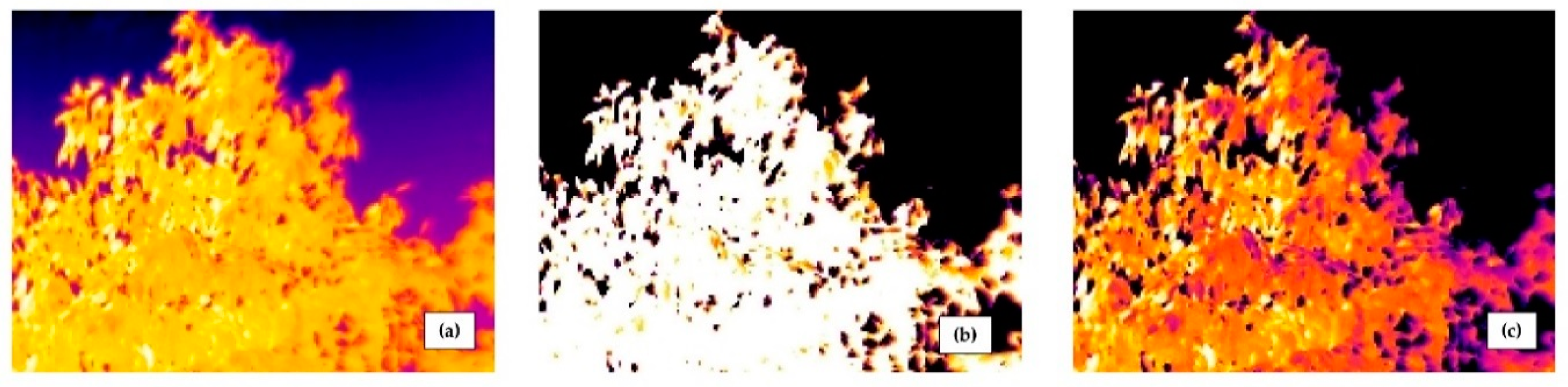
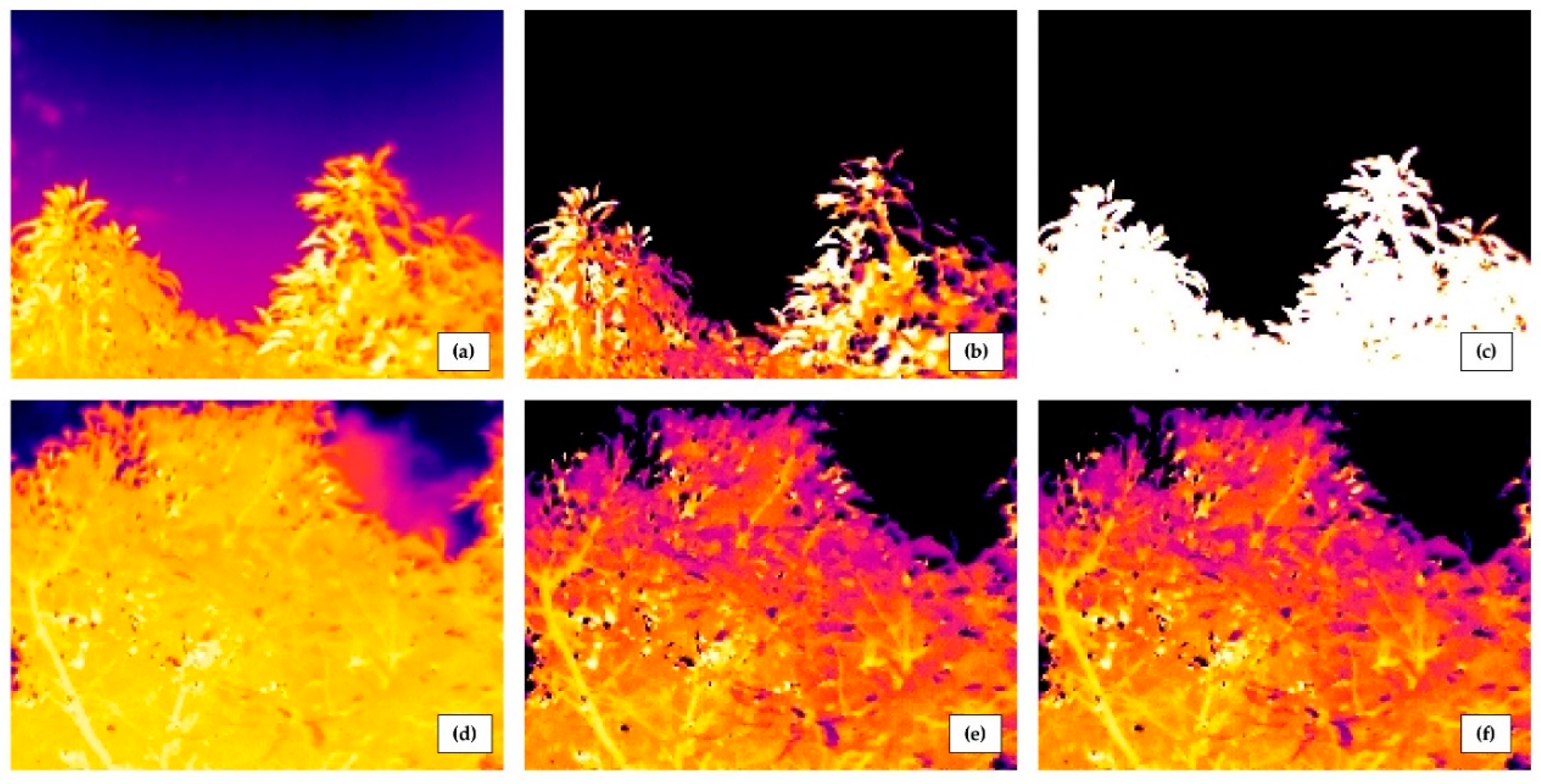
2.2.1. Canopy Images: Generating Temperature Histograms

In order to generate a temperature histogram for each image, the 510 FLIR JPEG images (pixels 320 × 240) of the 130 tree canopies (Figure 3a) were initially saved as 16 bit PNG images before the data values were extracted as image digital numbers (DN) using ‘Exiftool’ in R (RStudio 1.1, Inc., Austria) [17]. The DN images were then rectified using the ImageMagick® 7.0 (ImageMagick Studio, LLC) function in the command line from R, and then converted to temperature (degrees Celsius), assuming a surface emissivity of 0.98 for natural vegetation [18] and applying the measured object distance, relative humidity, and ambient temperature. Images were processed in R [16] using the ‘EBImage’ package [19] with a 2D matrix (200 × 150) of temperature values in .CSV file format generated for each image to support further processing (Figure 3b).

A custom code [16] written in MATLAB read each .CSV file and constructed histograms by re-organising the temperature pixel values from each file into equal-interval class bins (one degree Celsius) and calculating pixel number % (number of temperature pixels as a percentage of total image pixels) for each class. The 1 °C interval of class bins was considered as optimal to avoid over fitting the histogram shape and smoothing of important features [20]. Histogram values were normalised to 0% to 100% and the x-axis range was standardised to −30 to 70 °C for all the images. The resultant temperature histograms were typically unimodal (Figure 3c). The peak (mode) and main body of the histogram was assumed to be associated with the temperature profile of the tree canopy pixels, whilst lower and upper ‘tails’ of the histogram were assumed to correspond to the sky and non-leaf (namely non-transpiring) material pixels, respectively (Figure 3a,c).

2.2.2. Reference Surfaces: Deriving Temperatures T_wetRef and T_dryRef

The average surface temperatures T_wetRef and T_dryRef, from the ‘wet’ and ‘dry’ references, were extracted using FLIR ThermaCAM^™ researcher Pro 2.10 software (FLIR Systems, USA). Polygons were manually drawn within the extents of the reference leaves, and emissivity was set to 0.98 as the surfaces were of natural leaves [18], an approach consistent with that reported by Fuentes et al. [7] and Jones et al. [6] (Figure 2b). As these images were acquired in sequence, a time-based interpolation between these images was carried out to derive corresponding T_wetRef and T_dryRef for those trees that were imaged without the referenced panels included in the FOV. The time-based interpolation was used to account for any changes in evapotranspiration demand (for example, as effected by ambient temperature, relative humidity, and wind speed) that may have occurred to the trees during the image acquisition windows. To achieve this, a polynomial curve was fitted (poly 1 or 2) to existing referenced temperature values with time, using the ‘polyfit()’ function in MATLAB^® 2017a (MathWorks Inc., USA) and the T_wetRef and T_dryRef values extracted from the curve corresponding to the image acquisition time of those non-referenced trees.

2.3. Canopy Pixels Thresholding and Obtaining T_c

The value of T_c was obtained from the post-processed images using three methods, one of them being the conventionally (and widely) used standard reference method (using physical reference panels) [7]. Each of the methods was adopted using custom code [16] written in MATLAB^® 2017a (MathWorks Inc., USA). These methods were as follows:

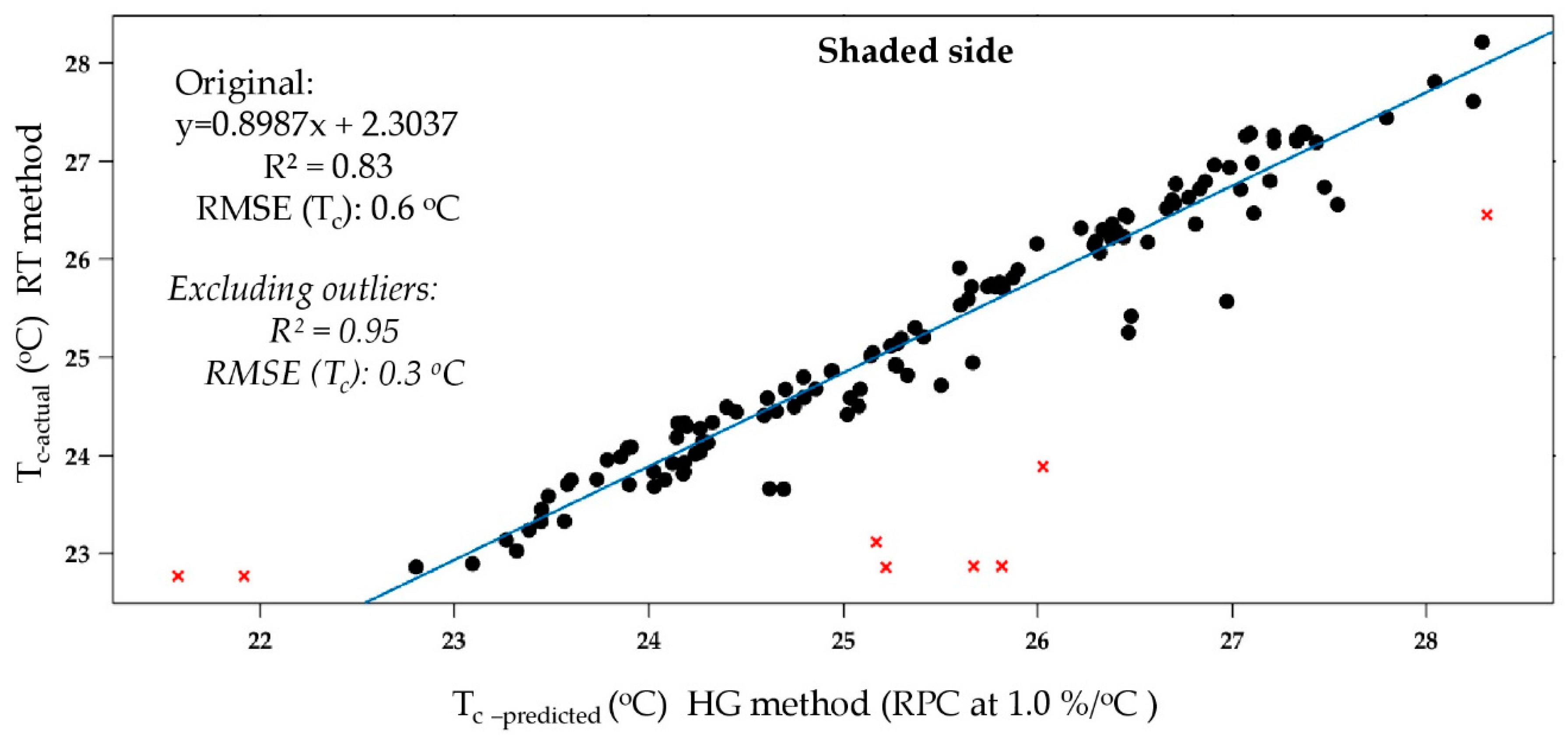
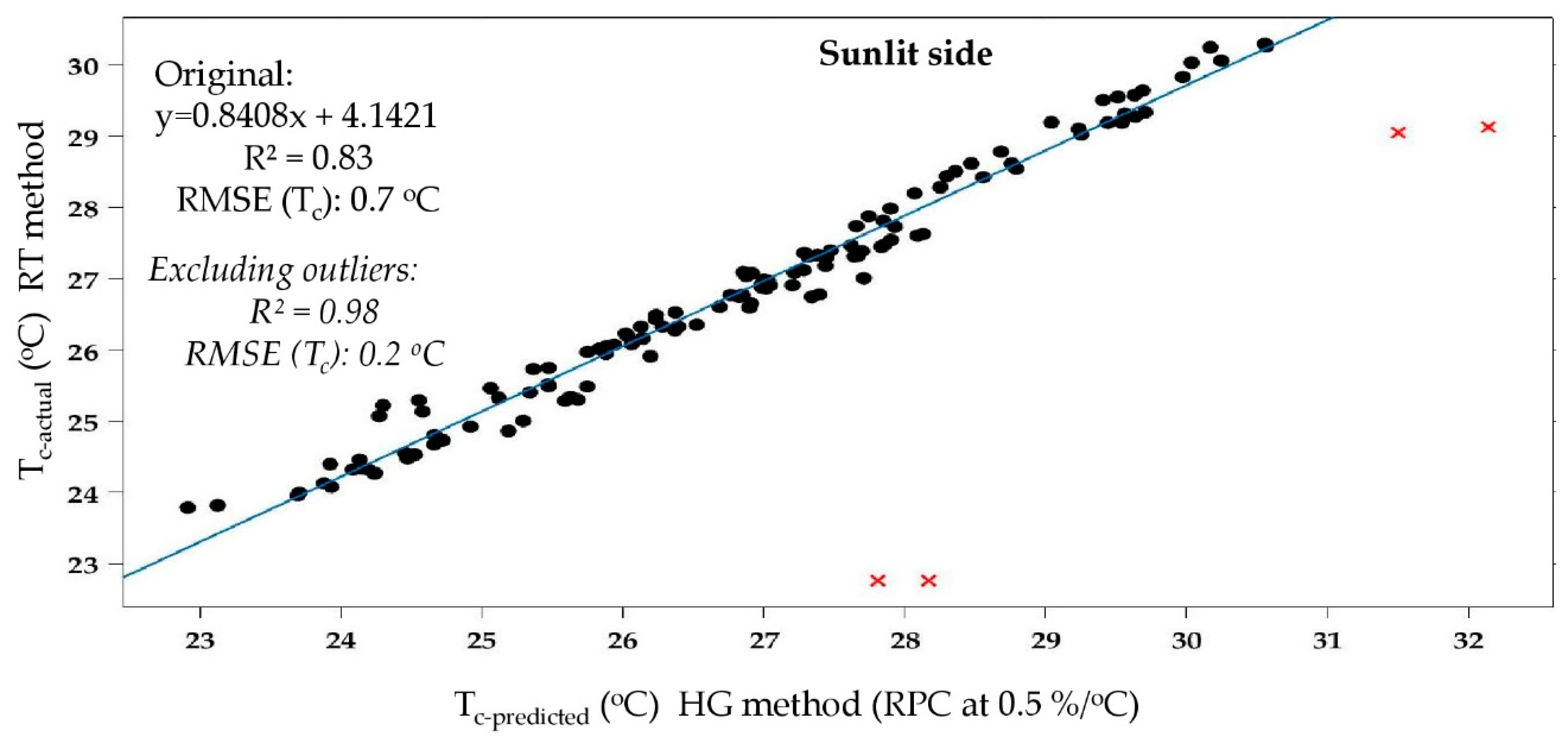
• Reference temperature (RT) thresholding: Using the derived temperature values T_wetRef and T_dryRef from the reference surfaces, all pixel values with temperatures lower than the T_wetRef or exceeding T_dryRef were removed [6,7], and from the remaining pixel values, the population average canopy temperature (T_c) was calculated for each tree. The T_c value for each tree (sunlit and shaded sides) was retained as the calibration/validation standard for the other two processing methods.
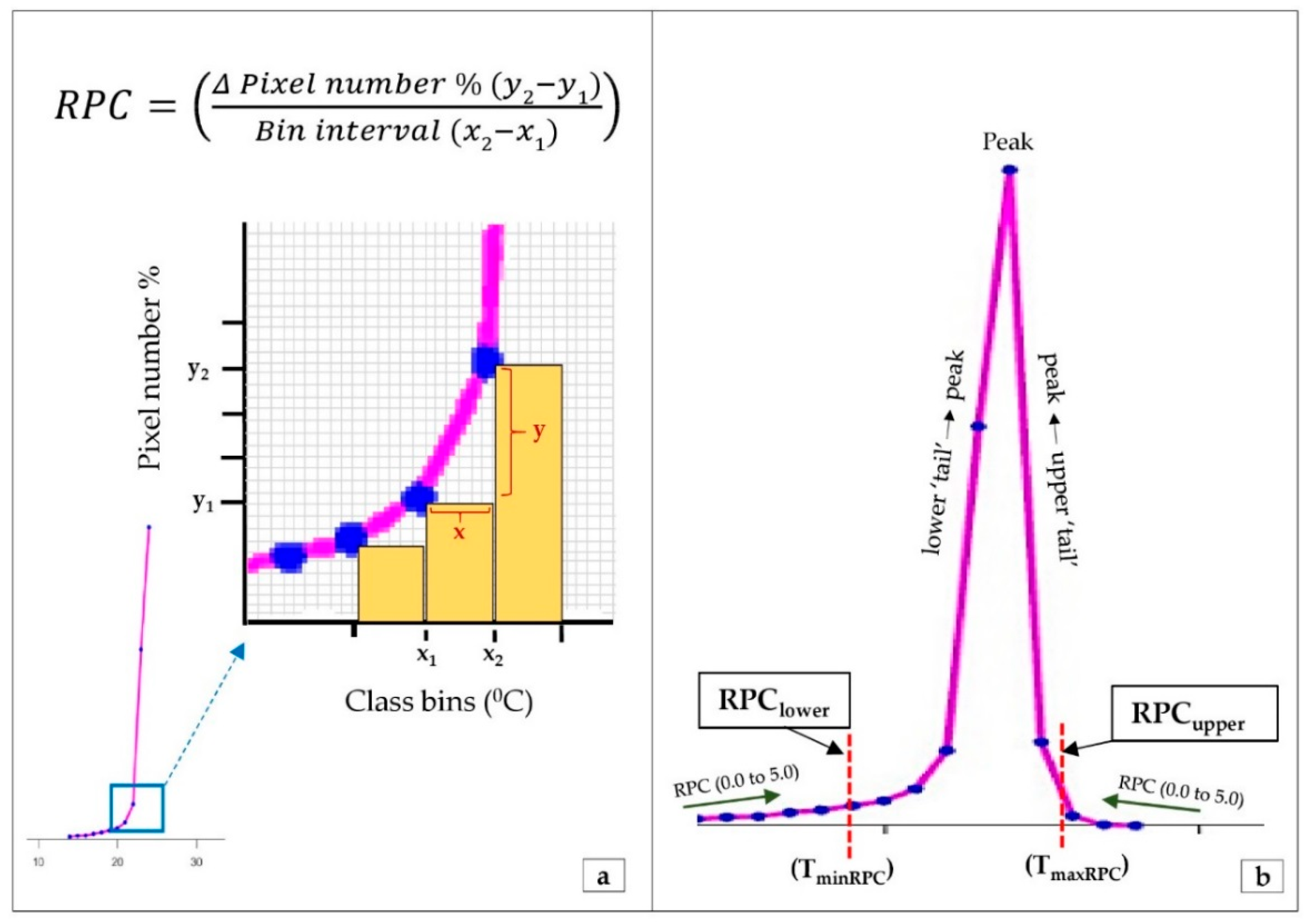
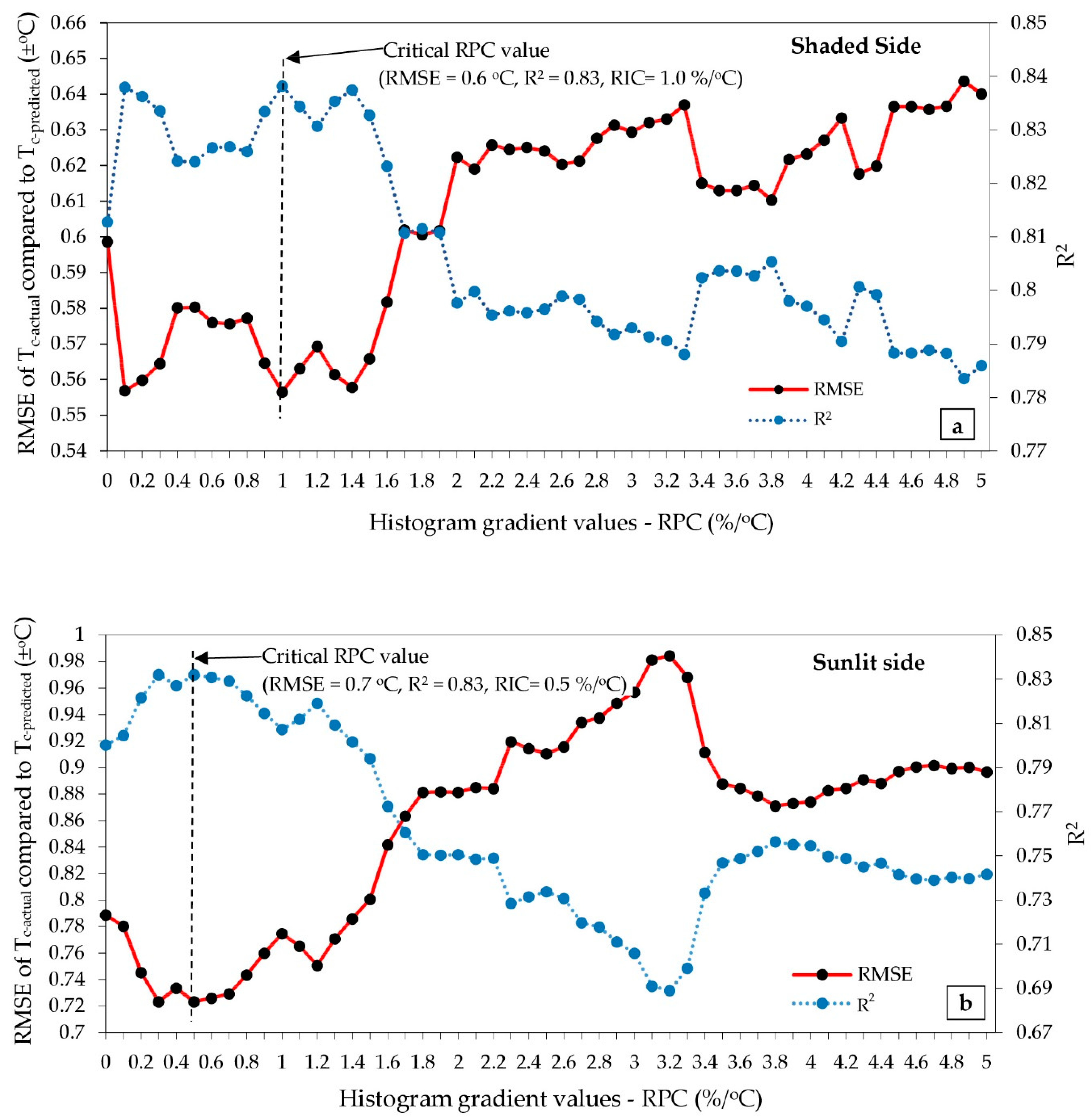
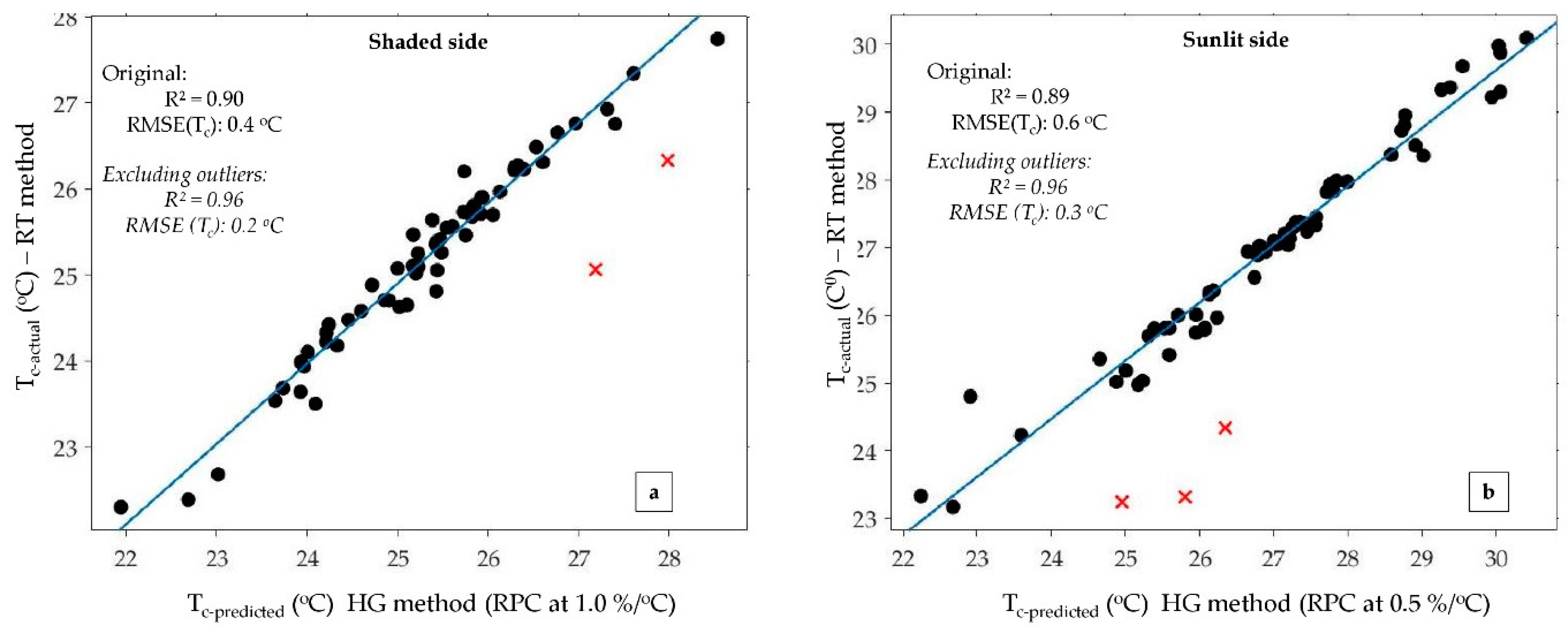
• Histogram gradient (HG) thresholding: This non-reference method is based on the identification of canopy upper and lower points (roughly corresponding to the T_dry and T_wet values, respectively) based on a pre-defined local gradient of the temperature histogram (Equation 1 and Figure 4a). Once assigned, the local gradient values, hitherto defined as ‘ratio pixel change—RPC’, were used to determine the corresponding temperature limits (RPC_lower → T_minRPC; RPC_upper → T_maxRPC) from which a value of T_c could be derived from the population average of the pixel temperatures between the two end values (Figure 4b). An iterative process was used to symmetrically and incrementally change the predefined gradient value from 0 %/°C (corresponding to the flat portions of the histogram tails) to the maximum gradient value (~50 %/°C). At each pair of RPC values, the value of T_c (T_c-predicted) was calculated as the population average and compared to the actual T_c value (T_c-actual) derived from the standard RT method above.

  $$\mathrm{Ratio}\mathrm{pixel}\mathrm{change}\left(\mathrm{RPC}\right)=\frac{\mathsf{\Delta }\mathrm{pixel}\mathrm{number}\%}{\mathrm{Class}\mathrm{bin}\mathrm{interval}}$$

  (1)
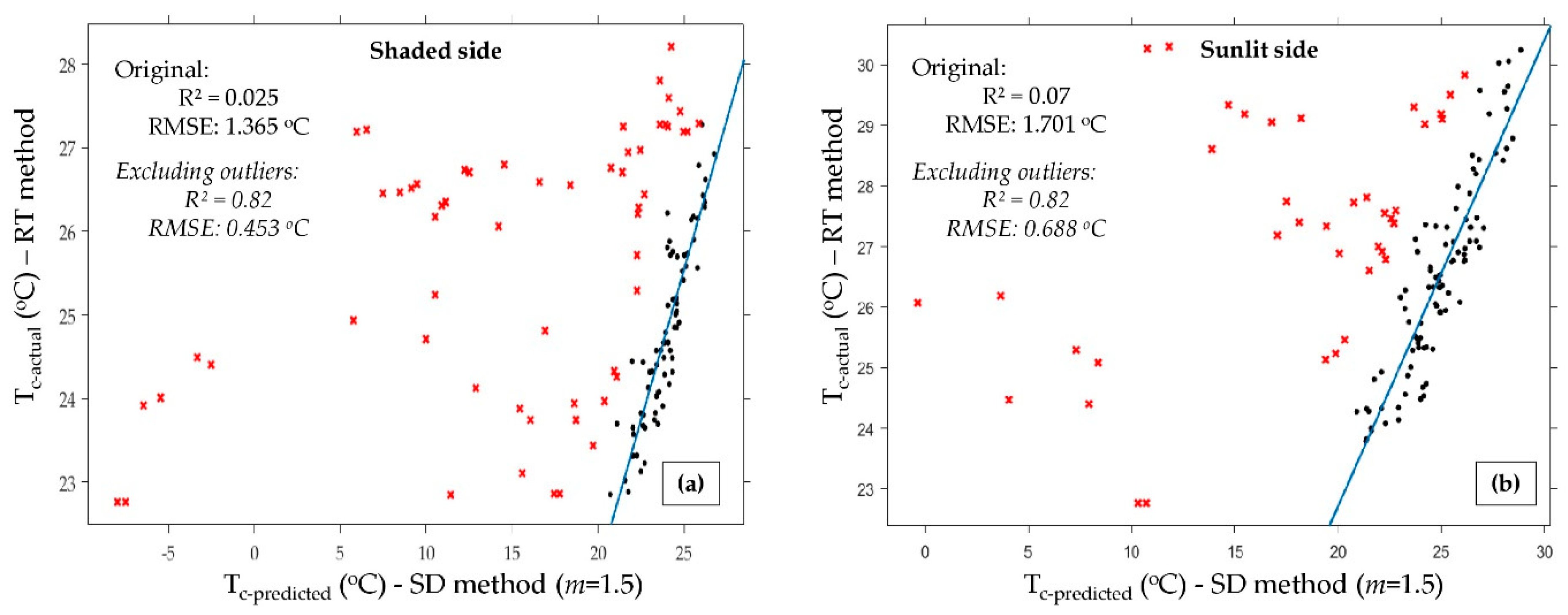
• Standard deviation (SD) envelope thresholding: This is a non-reference method based on the standard deviation envelope filtering method of Sepúlveda-Reyes et al. [5]. In each temperature data file, the canopy T_min (T_wet) and T_max (T_dry) were assumed to be a numeric multiplier (m) of the standard deviation (SD) above and below the unfiltered mean temperature (T_nf), respectively. The multiplier values ranged from m = ±0.0 (T_nf) through to ±2.0 (corresponding to the maximum and minimum values of the temperature file). Again, T_c-predicted was calculated as the population average value between T_min and T_max for each number m and compared to the standard RT method above.

2.4. Statistical Analysis

Each of the two non-reference methods (HG and SD) required iterations to determine the optimum value of the conditioning parameter, namely RPC or m, respectively. In order to determine these optimum values, 357 of the 510 images were used to ‘calibrate’ the methods insofar as producing T_c-predicted as a function of RPC or m for comparison with the reference-derived T_c-actual values of the same trees. The optimum values of RPC or m were then identified on the basis of the minimum root mean square error (RMSE). Furthermore, to select the best method of predicting T_c, T_c-predicted was derived again by each method (HG and SD) at their optimum RPC and m, respectively, and a linear regression analysis was performed with the corresponding T_c-actual values (using ‘fitlm()’ function in Curve Fitting Toolbox^® in MATLAB), from which R² and root mean square error (RMSE) were derived. The best method with strong correlation (R²) and minimum RMSE was then further validated using the remaining 153 images.

3. Results

3.1. Histogram Gradient Determination of T_c

The result of iterating the RPC values from 0 to 50.0 %/°C on the derived value of T_c (T_c-predicted) is depicted in Figure 5a,b for shaded and sunlit sides of the tree canopy, respectively (only RPC range 0 to 5.0 %/°C is shown for clear illustration). Here, the RMSE and R² values are plotted as a function of the tested RPC values. It is noteworthy that in both Figure 5a,b, there exist two obvious minima: In Figure 5a (0.1 %/°C and 1.0 %/°C), and the similar (although less distinct) minima in Figure 5b (0.3 %/°C and 0.5 %/°C). The lower-valued minima of each graph correspond to temperature bin numbers closer to the extremes of the histograms, namely the blue sky (lower end) and non-photosynthetic material/sun-glint (higher end). Given the likelihood that these pixels are non-canopy related (allowing for sun-glint from the shiny leaf surfaces to be included here), then the upper of the two minima should be used in each case. Consequently, for the shaded-side images, the lowest RMSE (T_c) (±0.6 °C) and highest R² (0.83) were reported when T_c was obtained at RPC 1.0 %/°C (Figure 5a). For the sunlit-side images, the lowest RMSE (T_c) (±0.7 °C) and highest R² (0.83) occurred for T_c obtained at RPC 0.5 %/°C (Figure 5b).

An examination of the scatterplots (Figure 6 and Figure 7) of T_c-actual versus T_c-predicted for each of the optimum values of RPC (shaded: 1.0 %/°C; sunlit: 0.5 %/°C) reveals a strong linearity (R² = 0.83) although there are a small number of prominent outliers (marked in red).

Outliers were further evaluated by visually observing the threshold limits obtained by each method in FLIR ThermaCAM^™ researcher Pro 2.10 software (FLIR Systems, USA) (Figure 8). It was clear that the RT method had performed the incorrect thresholding by excluding a large proportion of the canopy pixels (white area) (Figure 8a), whereby the HG method canopy pixels were correctly thresholded (Figure 8c). This error reported by the RT method might be due to sudden environmental changes (e.g., wind, broken sunlight) which may result in alteration of actual T_c. The removal of these outliers increased the R² to 0.96 and 0.97 in both shaded and sunlit sides, respectively (Figure 6 and Figure 7).

3.2. Standard Deviation-Based Threshold Determination of T_c

From the result of iterating the m values from ±0.0 to ±2.0 on the derived value of T_c (T_c-predicted), at m = ±1.5 a minimum RMSE was recorded for both shaded- and sunlit-side images (results not shown). When examining the scatterplots (Figure 9a,b) of T_c-actual versus T_c-predicted for the optimum value of m = 1.5, poor correlations were revealed for both shaded and sunlit sides (shaded: R² = 0.02; sunlit: R² = 0.07) with a large number of outliers (marked in red).

It was found that the outliers corresponded with thermal images with partial canopy inclusions (Figure 10). When comparing Figure 10a–c, during a smaller canopy situation, thresholding was poorly performed by the SD method (exclusion of canopy: White area in Figure 10c). In the cases of large canopy situations (Figure 10d–f), the SD method was able to correctly threshold the canopy pixels (Figure 10f). The removal of these outliers increased the R² to 0.82 in both shaded and sunlit sides, respectively (Figure 9a,b).

A summary of the statistical results obtained for both shaded and sunlit sides by HG and SD methods are shown in

Table 1. Summary of statistical output of histogram gradient (HG) and standard deviation (SD) thresholding methods for obtaining T_c.

		Shaded			Sunlit
Total Images	Method	Optimum value	RMSE (Tc) ±°C	R2	Optimum Value	RMSE (Tc) ±°C	R2
357	HG	RPC at 1.0	±0.6	0.83	RPC at 0.5	±0.7	0.83
357	SD	Tnf ± (SD*1.5)	±1.4	0.02	Tnf ± (SD*1.5)	1.7	0.07

HG—histogram gradient method, RPC—ratio of pixels change, SD—standard deviation, T_nf—unfiltered mean temperature

.

The HG method was found to be far more accurate than the SD method in the prediction of T_c for both the shaded (R² = 0.83) and sunlit (R² = 0.83) sides of the tree (Table 1).

3.3. Validation Results

The results from the calibration work indicated the potential of the newly proposed HG thresholding method for predicting T_c. To validate this outcome, the analysis was repeated on additional canopy images. According to Figure 11a,b, strong linearity was observed for both shaded (R² = 0.90) and sunlit (R² = 0.89) side images, similarly to the calibration results. There were few outliers resulting from the error in T_{c_actual} (marked in red), where removal of them improved the correlation to R² = 0.96 for both sides (Figure 11a,b).

Therefore, the resulting ‘optimum thresholds’ for the HG method were found to be consistent with the threshold temperature histogram at RPC 1.0 %/°C and 0.5 %/°C for shaded and sunlit images, respectively. This was true even for different canopy sizes.

4. Discussion

In order to determine the average temperature of a tree canopy (T_c), it is necessary to remove non-canopy-related pixels, such as stem parts, sky, and leaves exhibiting specular reflection from thermal imagery. Historically, the inclusion of both T_wetRef and T_dryRef within each thermal image has been used to achieve this thresholding. Although effective, this method is time consuming and labour intensive, and therefore prohibitive to the collection of thermal information for many trees, i.e., commercial orchards at any one time. The histogram gradient (HG) method presented in this study offers a histogram method for thresholding canopy pixels from thermal images that produces results comparable to those from the accepted reference temperature (RT) thresholding method. The development of the unimodal histogram for each image and the subsequent removal of the left and right ‘tails’ (e.g., thresholding limits T_min and T_max of the canopy) successfully removed pixel information associated with non-canopy-related features. The consistency of histograms derived from each image was maintained by including the sky, without the sun disc or canopies from surrounding trees, in each image. The consistent angle of view and 4 m distance between the camera and the tree canopy also supported a standardised spatial scaling.

The FLIR B250 camera has a low IR resolution of 200 × 150 pixels, which may result in a lesser number of pixels of the target than could be obtained from a high-resolution camera. However, the proposed method should be applicable even across different camera resolutions as far as the histogram is constructed with one degree Celsius class bins and the number of pixels per class bin is presented as a percentage of the total number of pixels in the image.

Whilst Sepúlveda-Reyes et al. [5] achieved encouraging results using the SD method for thresholding aerial thermal images of tree canopies, the same result was not achieved in this study using ground-based thermal images. This may be due to the temperature histograms from ground thermal images being skewed left (Figure 3c) due to the inclusion of lower-temperature pixels from the sky. Furthermore, a Gaussian mixture method was previously suggested by Wang et al. [3] to derive T_c from ground thermal images, but it required the temperature pixel distribution to be normalised, which was not required in this HG method.

The limitations of the new HG thresholding method are that it requires the maintenance of consistency during image acquisition (viewing angle, distance to tree, and clear sky), and the background temperature must be distinguishable (either low or high) from canopy temperature. As a future improvement, additional non-reference procedures based on histogram thresholding could be tested. This may include Gaussian mixture distribution extraction [3,21], colour intensity histograms [22], or using deep machine learning algorithms such as convolution neural networks [23]. Additionally, in future the performance of the new method should be evaluated over tree species other than avocado, different environmental situations such as early morning and late afternoon, cloudy conditions, and on different platforms such as mounted on a ground vehicle

However, the histogram gradient threshold presents as a new and easy way of thresholding canopy pixels in ground canopy thermal imagery, enabling the monitoring of individual trees for changes in water status caused by abiotic and biotic factors. Therefore, this method offers great benefit to future agriculture processes (precision farming) that rely on large volumes of thermal remotely sensed imagery.

5. Conclusions

The results from this study present an alternative, histogram method for thresholding canopy area from ground-based thermal imagery without the need of temperatures from reference surfaces. By developing a unimodal histogram for each image and then removing the left and right ‘tails’ associated with non-canopy-related features based on histogram gradients (e.g., T_wet and T_dry boundaries) predictions of average canopy temperature (T_c) were achieved. These predictions of T_c were found to be highly comparable to T_c produced from the commonly used method (reference temperature thresholding), which requires the inclusion of physical ‘wet’ and ‘dry’ references within each image. This novel ‘histogram gradient thresholding’ method offers a more time-efficient and labour-saving method, and is a potentially automated method of calculating canopy temperature from thermal imagery, allowing large volumes of images to be processed in a short time. This result was not previously possible with either the reference method or the manual digitisation of canopy specific pixels within each image. With the ever increasing interest in remote sensing technologies for monitoring tree health, this outcome offers significant benefit for the rapid and standardised analysis of thermal imagery.

References

1. Mahlein, A.-K. Plant Disease Detection by Imaging Sensors—Parallels and Specific Demands for Precision Agriculture and Plant Phenotyping. Plant Dis. 2016, 100, 241–251. [Google Scholar] [CrossRef] [PubMed]
2. Stoll, M.; Schultz, H.R.; Baecker, G.; Berkelmann-Loehnertz, B. Early pathogen detection under different water status and the assessment of spray application in vineyards through the use of thermal imagery. Precis. Agric. 2008, 9, 407–417. [Google Scholar] [CrossRef]
3. Wang, X.; Yang, W.; Wheaton, A.; Cooley, N.; Moran, B. Automated canopy temperature estimation via infrared thermography: A first step towards automated plant water stress monitoring. Comput. Electron. Agric. 2010, 73, 74–83. [Google Scholar] [CrossRef]
4. Poblete-Echeverría, C.; Ortega-Farías, S.; Lobos, G.A.; Romero, S.; Ahumada, L.; Escobar, A.; Fuentes, S. Non-invasive method to monitor plant water potential of an olive orchard using visible and near infrared spectroscopy analysis. Acta Hortic. 2014, 363–368. [Google Scholar] [CrossRef]
5. Sepúlveda-Reyes, D.; Ingram, B.; Bardeen, M.; Zúñiga, M.; Ortega-Farías, S.; Poblete-Echeverría, C. Selecting Canopy Zones and Thresholding Approaches to Assess Grapevine Water Status by Using Aerial and Ground-Based Thermal Imaging. Remote Sens. 2016, 8, 822. [Google Scholar] [CrossRef]
6. Jones, H.G.; Stoll, M.; Santos, T.; de Sousa, C.; Chaves, M.M.; Grant, O.M. Use of infrared thermography for monitoring stomatal closure in the field: Application to grapevine. J. Exp. Bot. 2002, 53, 2249–2260. [Google Scholar] [CrossRef] [PubMed]
7. Fuentes, S.; De Bei, R.; Pech, J.; Tyerman, S. Computational water stress indices obtained from thermal image analysis of grapevine canopies. Irrig. Sci. 2012, 30, 523–536. [Google Scholar] [CrossRef]
8. Cohen, Y.; Alchanatis, V.; Meron, M.; Saranga, Y.; Tsipris, J. Estimation of leaf water potential by thermal imagery and spatial analysis. J. Exp. Bot. 2005, 56, 1843–1852. [Google Scholar] [CrossRef] [PubMed]
9. García-Tejero, I.; Ortega-Arévalo, C.; Iglesias-Contreras, M.; Moreno, J.; Souza, L.; Tavira, S.; Durán-Zuazo, V. Assessing the Crop-Water Status in Almond (Prunus dulcis Mill.) Trees via Thermal Imaging Camera Connected to Smartphone. Sensors 2018, 18, 1050. [Google Scholar] [CrossRef] [PubMed]
10. Leinonen, I.; Jones, H.G. Combining thermal and visible imagery for estimating canopy temperature and identifying plant stress. J. Exp. Bot. 2004, 55, 1423–1431. [Google Scholar] [CrossRef] [PubMed]
11. Moller, M.; Alchanatis, V.; Cohen, Y.; Meron, M.; Tsipris, J.; Naor, A.; Ostrovsky, V.; Sprintsin, M.; Cohen, S. Use of thermal and visible imagery for estimating crop water status of irrigated grapevine. J. Exp. Bot. 2006, 58, 827–838. [Google Scholar] [CrossRef] [PubMed]
12. Costa, J.M.; Grant, O.M.; Chaves, M.M. Thermography to explore plant–environment interactions. J. Exp. Bot. 2013, 64, 3937–3949. [Google Scholar] [CrossRef] [PubMed]
13. Jones, H.G. Use of infrared thermometry for estimation of stomatal conductance as a possible aid to irrigation scheduling. Agric. For. Meteorol. 1999, 95, 139–149. [Google Scholar] [CrossRef]
14. García-Tejero, I.; Durán-Zuazo, V.H.; Arriaga, J.; Hernández, A.; Vélez, L.M.; Muriel-Fernández, J.L. Approach to assess infrared thermal imaging of almond trees under water-stress conditions. Fruits 2012, 67, 463–474. [Google Scholar] [CrossRef]
15. Salgadoe, S.; Robson, A.; Lamb, D.; Dann, E.; Searle, C. Quantifying the Severity of Phytophthora Root Rot Disease in Avocado Trees Using Image Analysis. Remote Sens. 2018, 10, 226. [Google Scholar] [CrossRef]
16. Thermal Image_processing. Available online: https://gitlab.une.edu.au/asalgado/thermalimage_processing/tree/Master (accessed on 22 February 2019).
17. Dunnington, D.; Harvey, P. exifr: EXIF Image Data in R. R Package Version 0.1.1, 2016.
18. Calderón, R.; Navas-Cortés, J.; Zarco-Tejada, P. Early Detection and Quantification of Verticillium Wilt in Olive Using Hyperspectral and Thermal Imagery over Large Areas. Remote Sens. 2015, 7, 5584–5610. [Google Scholar] [CrossRef]
19. Pau, G.; Fuchs, F.; Sklyar, O.; Boutros, M.; Huber, W. EBImage—An R package for image processing with applications to cellular phenotypes. Bioinformatics 2010, 26, 979–981. [Google Scholar] [CrossRef] [PubMed]
20. Lindblad, J. Histogram thresholding using kernel density estimates. In Proceedings of the Swedish Society for Automated Image Analysis (SSAB) Symposium on Image Analysis, Halmstad, Sweden, March 2000; pp. 41–44. [Google Scholar]
21. Raza, S.-A.; Smith, H.K.; Clarkson, G.J.J.; Taylor, G.; Thompson, A.J.; Clarkson, J.; Rajpoot, N.M. Automatic Detection of Regions in Spinach Canopies Responding to Soil Moisture Deficit Using Combined Visible and Thermal Imagery. PLoS ONE 2014, 9, e97612. [Google Scholar] [CrossRef] [PubMed]
22. Yang, N.; Yuan, M.; Wang, P.; Zhang, R.; Sun, J.; Mao, H. Tea Diseases Detection Based on Fast Infrared Thermal Image Processing Technology. J. Sci. Food Agric. 2019. [Google Scholar] [CrossRef] [PubMed]
23. De Oliveira, D.; Wehrmeister, M. Using Deep Learning and Low-Cost RGB and Thermal Cameras to Detect Pedestrians in Aerial Images Captured by Multirotor UAV. Sensors 2018, 18, 2244. [Google Scholar] [CrossRef] [PubMed]
Figure 1. Flow diagram of methodologies used in the study; HG—histogram gradient thresholding, SD—standard deviation envelope thresholding, and RT—reference temperature thresholding.
Remotesensing 11 00714 g001
Figure 2. ‘Dry’ and ‘wet’ reference surfaces. (a) Practical implementation of the panel with reference surfaces; (b) extracting temperature by manually drawn polygons on thermal image.
Remotesensing 11 00714 g002
Figure 3. Sequence of canopy thermal image processing; (a) original thermal imagery (blue: Sky area; yellow: Tree canopy, bright yellow: Non-leaf material), (b) extracted temperature matrix, (c) unimodal histogram of the temperature matrix, and (d) pictorial interpretation of a threshold thermal image (black: Excluded sky area; white area: Excluded hot stem parts; and colored: Leaf material).
Remotesensing 11 00714 g003
Figure 4. Graphical interpretation of the histogram gradient thresholding (HG) technique; (a) calculating ratio pixel change (RPC) in the lower ‘tail’, (b) RPC points with corresponding temperature bin values.
Remotesensing 11 00714 g004
Figure 5. Root mean squared error (RMSE) and R2 of Tc reported by the histogram gradient (HG) method at different RPC gradients tested in the histogram for (a) shaded-side and (b) sunlit-side images.
Remotesensing 11 00714 g005
Figure 6. Shaded-side image thresholding for Tc, HG vs reference temperature (RT) method.
Remotesensing 11 00714 g006
Figure 7. Sunlit-side image thresholding for Tc, HG vs reference temperature (RT) method.
Remotesensing 11 00714 g007
Figure 8. Pictorial representation of outliers (HG vs RT thresholding); (a) original thermal image (coloured: canopy and sky), (b) incorrect threshold by RT method (white: canopy incorrectly excluded; black: excluded sky), (c) correct threshold by HG method (coloured: canopy; black: excluded sky).
Remotesensing 11 00714 g008
Figure 9. Thresholding for Tc. Standard deviation (SD) method vs reference tempererature (RT) thresholding; (a) shaded-side images, (b) sunlit-side images.
Remotesensing 11 00714 g009
Figure 10. Comparison of outliers (SD method vs RT method); smaller canopy situation (a, b, and c); (a) original thermal image (coloured: canopy and sky), (b) correct threshold by RT method (coloured: canopy; black: excluded sky), (c) incorrect threshold by SD method (white: canopy incorrectly excluded; black: excluded sky). Larger canopy situation (d, e, and f); (d) original thermal image (coloured: canopy and sky), (e) correct threshold by RT method (coloured: canopy; black: excluded sky), (f) correct threshold by SD method (coloured: canopy; black: excluded sky).
Remotesensing 11 00714 g010
Figure 11. Validation results of Tc from the HG method; (a) shaded-side images, (b) sunlit-side images.
Remotesensing 11 00714 g011