Determining the AMSR-E SST Footprint from Co-Located MODIS SSTs


1
Graduate School of Oceanography, University of Rhode Island, 215 South Ferry Road, Narragansett, RI 02882, USA
2
Department of Computer Science and Statistics, University of Rhode Island, 9 Greenhouse Road, Suite 2, Kingston, RI 02881, USA
3
Earth and Space Research, Seattle, WA 98121, USA
*
Author to whom correspondence should be addressed.
Remote Sens. 2019, 11(6), 715; https://0-doi-org.brum.beds.ac.uk/10.3390/rs11060715
Submission received: 19 February 2019
/
Revised: 10 March 2019
/
Accepted: 21 March 2019
/
Published: 25 March 2019
(This article belongs to the Special Issue Sea Surface Temperature Retrievals from Remote Sensing)
Abstract
:This study was undertaken to derive and analyze the advanced microwave scanning radiometer-Earth observing satellite (EOS) (AMSR-E) sea surface temperature (SST) footprint associated with the remote sensing systems (RSS) level-2 (L2) product. The footprint, in this case, is characterized by the weight attributed to each km square contributing to the SST value of a given (AMSR-E) pixel. High-resolution L2 SST fields obtained from the moderate-resolution imaging spectroradiometer (MODIS), carried on the same spacecraft as AMSR-E, are used as the sub-resolution “ground truth” from which the AMSR-E footprint is determined. Mathematically, the approach is equivalent to a linear inversion problem, and its solution is pursued by means of a constrained least square approximation based on the bootstrap sampling procedure. The method yielded an elliptic-like Gaussian kernel with an aspect ratio ≈1.58, very close to the AMSR-E channel aspect ratio, ≈1.74. (The channel is the primary spectral frequency used to determine SST.) The semi-major axis of the estimated footprint is found to be aligned with the instantaneous field-of-view of the sensor as expected from the geometric characteristics of AMSR-E. Footprints were also analyzed year-by-year and as a function of latitude and found to be stable—no dependence on latitude or on time. Precise knowledge of the footprint is central for any satellite-derived product characterization and, in particular, for efforts to deconvolve the heavily oversampled AMSR-E SST fields and for studies devoted to product validation and comparison. A preliminary analysis suggests that use of the derived footprint will reduce the variance between AMSR-E and MODIS fields compared to the results obtained ignoring the shape and size of the footprint as has been the practice in such comparisons to date.

SST NASA
1. Introduction
Sea surface temperature (SST), one of the ten ocean surface essential climate variables (ECVs) [1], is measured from satellite-borne sensors in both the microwave portion of the electromagnetic spectrum and the infrared portion of the spectrum. The current generation of infrared instruments provide very high-resolution, , SST fields contributing significantly to the study of small scale features at the ocean surface and their impact on large scale phenomena [2]. However, infrared radiometers only supply an SST estimate when they view the sea surface under cloud-free skies. This limitation severely reduces the coverage of the global oceans by infrared sensors, coverage that is strongly dependent on location and season, with some areas experiencing cloud free conditions less than 5% of the time for extended periods (months). By contrast, with the exception of regions of heavy rainfall, the atmosphere is relatively transparent to radiation in significant portions of the microwave spectrum; i.e., SST retrievals through clouds are possible with satellite-borne instruments measuring in the microwave. The downside of microwave SST retrievals is that to achieve a reasonable accuracy, the sensor must sample a large area—the spatial resolution of these fields is generally quite coarse, . Another important characteristic of SST fields derived from extant microwave sensors is the large overlap in pixels. As will be discussed below (Section 2.1) the sensors of interest sample approximately every 10 km in both the along- and across-track directions, while the radiometer footprint is . These two characteristics of microwave SST retrievals, large pixel size and significant overlap in adjacent pixels, lead to some interesting problems/possibilities, one related to instrument-to-instrument comparisons and the other to enhanced resolution of the microwave SST field.
Microwave-to-infrared SST comparisons. Of interest to the work presented herein are two sensors, the advanced microwave scanning radiometer-Earth observing satellite (EOS) (AMSR-E), a microwave instrument, and the moderate-resolution imaging spectroradiometer (MODIS), an infrared instrument, both carried on the National Aeronautics and Space Administration’s (NASA’s) Aqua satellite, launched in May 2002 [3]. The collocation of these two instruments on the same satellite platform offers the interesting possibility of providing passive microwave and infrared radiometer data, and SST fields retrieved from these data, very nearly simultaneously. A number of investigators have taken advantage of this to compare the performance of the two instruments, e.g., [4,5,6]. This has been done in the context of AMSR-E/MODIS matchup datasets, sets of high quality, simultaneous retrievals from the two instruments. However, in their analyses of these matchup datasets, the authors of these studies did not take into account the mismatch in the shape and size of the region sampled by each sensor. Specifically, one must average the higher resolution MODIS SSTs to the AMSR-E grid (the coarsest grid) at a similar spatial resolution in order to eliminate the MODIS high spatial variability. Given that the power spectral density of SST in the open ocean decreases linearly in log-log space with a slope of [7,8], the variation of SST is a factor of 50 or more on the scale of microwave SST pixels as it is on the scale of infrared pixels. This means that SST can vary significantly from one MODIS sized region in the AMSR-E pixel to another when compared to the variation within a MODIS pixel—ignoring the shape and size of the AMSR-E SST pixel will overestimate the root-mean-square difference between the two observations.
Enhanced spatial resolution. The AMSR-E SST retrieval algorithms developed by remote sensing systems (RSS), provide SST on a 10 km grid for their L2 products and on a 25 km for their L3 product, but the region contributing to the recorded SST at each of these grid locations is, as noted above, thought to be . This means that each point in the ocean is seen by pixels. It should therefore be possible to deconvolve the AMSR-E SST field yielding a true 10 km product.
The AMSR-E footprint. In both of the cases outlined above, an accurate estimate of the shape and size of the region contributing to the AMSR-E SST retrievals will benefit the analyses. For example, the use of a footprint (the weighting function mapping the temperature distribution at the ocean surface to a retrieved SST value) that is not representative of the AMSR-E SST product will result in artifacts in the differences between AMSR-E SST fields and MODIS SST, increasing the variance of the difference, as will be shown. Microwave SST data deconvolution also requires incorporation of the footprint to meet the demand for optimal reconstruction; selecting an appropriate footprint is a key preliminary step. For instance, the procedure described in [9] is based on the knowledge of the footprint measurement model.
To the best of our knowledge there are no published studies detailing the shape of the AMSR-E SST footprint, although the footprints size is commonly referred to as ranging from 50 km [10] to 58 km, with the most common reference to 56 km [2], close to the average of the axes of the footprint. The objective of the work presented herein is to determine the shape of the AMSR-E SST footprint and any dependencies that it might have on cell position, latitude, and time. From the perspective of this study, it is important to recognize the distinction between the footprint of a given channel of an instrument and the footprint of the retrieved SST values, which may depend on more than one spectral channel (discussed in Section 2.1), each with its own footprint, and/or on additional processing, such as averaging.
2. Data
2.1. AMSR-E
AMSR-E was a National Space Development Agency (Japan) (NASDA) instrument launched on the Aqua satellite in May 2002. It failed when its antenna stopped rotating in October 2011. AMSR-E was a dual-polarized, conical-scanning, passive microwave radiometer. The wide swath (1450 km) of the instrument and the near-polar orbit in which it was flown provided near global coverage twice daily, once on the sun-side of Earth (daytime, ascending, 1330 local Sun time (LST)) and once on the dark side (nighttime, descending, 0130 LST). AMSR-E, a twelve channel instrument, measured the vertical and horizontal polarization in each of six frequency bands. The AMSR-E antenna footprint, which was unique for each channel and increased with decreasing frequency, was determined by the antenna gain pattern [11]. The antenna gain pattern footprint describes how much the emissions from a particular receive direction contributes to the observed value. The Japan Aerospace Exploration Agency (JAXA) provided measured antenna patterns for the AMSR-E sensor at all center frequencies. The nominal size of the footprint for each of the spectral bands is reproduced from [11] in Table 1. For additional details with regard to the footprint, please see [12]. As noted in the introduction, there is likely a difference between the SST footprint and the footprint of the primary spectral channel contributing to the retrieval.
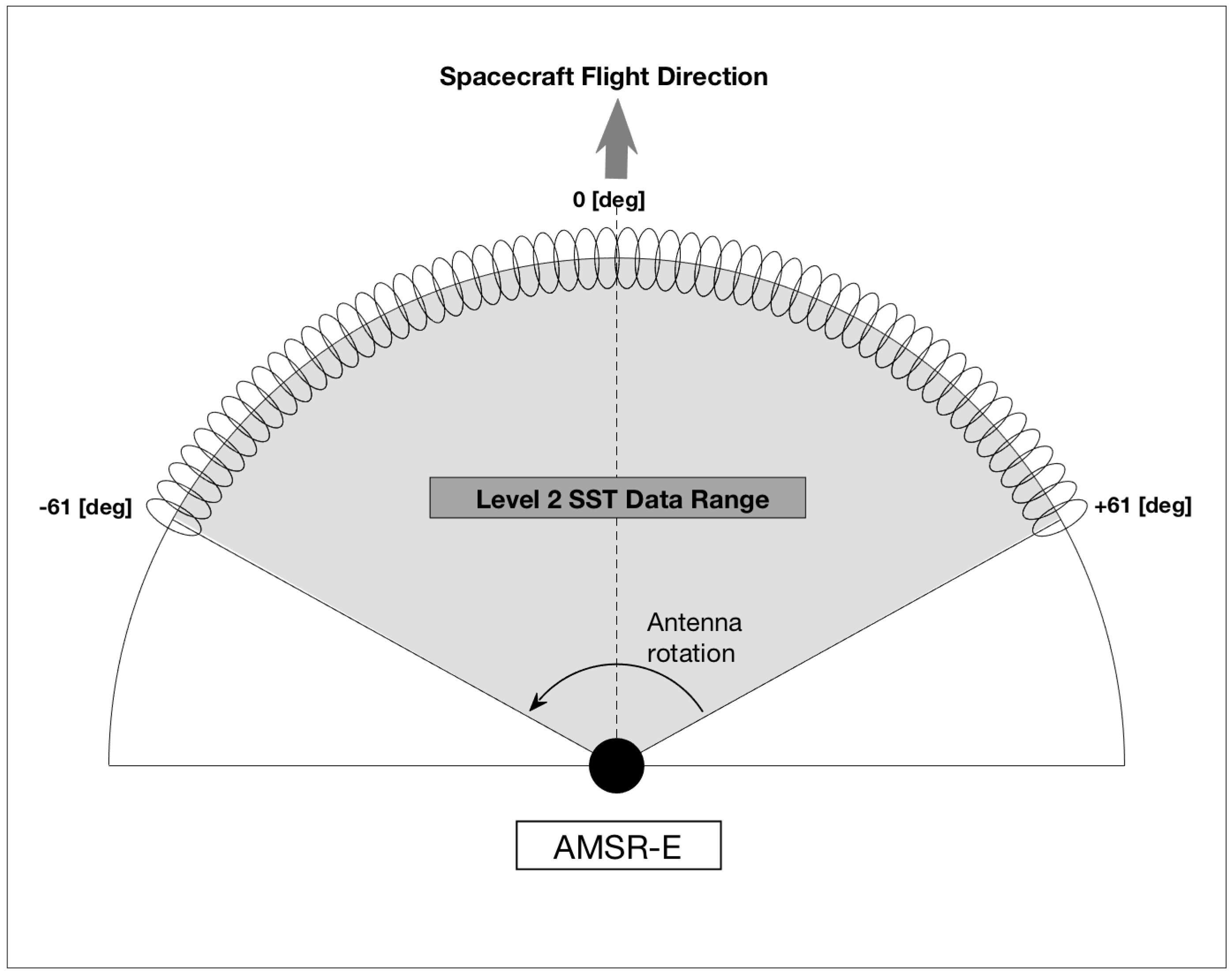
The scan geometry of the instrument in orbit is shown in Figure 1. The satellite orbit height was 705 km, the ground incidence angle was 55°, and the observation angle range was from –61° to +61°. In one scan, AMSR-E sampled 243 cell footprints for each of the frequency bands except for the 89 GHz band, for which it sampled at twice the frequency.
In this study, we use SST fields obtained with version-7 (v7) of the AMSR-E algorithm developed by RSS. The data were acquired from the Physical Oceanography-Distributed Active Archive Center (PO-DAAC) server at: https://podaac.jpl.nasa.gov. This algorithm simultaneously determines water vapor, cloud liquid water, precipitation, sea surface WS and SST using brightness temperature measurements from all spectral channels except for those at 89 GHz. SST, the variable of interest here, is derived primarily from the 6.93 GHz channel. As shown in Table 1, the ground resolution of the channel was approximately 75 km in the direction defined by a vector from the pixel to the nadir point of the satellite and approximately 43 km normal to this vector [11]. Thus, the retrieved SST was of coarse spatial resolution. The distance between adjacent observations for all channels, except those of 89 GHz, was approximately 10 km across-track and 10 km along-track [11]; i.e., the 6.93 GHz channel was substantially oversampled, with the remaining channels being less so. (Note that because the AMSR-E antenna rotates about a vertical axis with a beam direction 47.5 relative to this axis, a scan-line describes an approximate circle on the Earth’s surface so, as one moves away from nadir, the across-track direction was not orthogonal to the along-track direction.) To work simultaneously with all spectral channels, the RSS retrieval algorithm resampled the brightness temperatures for each of the spectral channels to match the resolution of the 6.93 GHz channel [13]. The SST was then retrieved using a physically based two-stage regression algorithm that expresses SST in terms of the resampled brightness temperatures (see the Appendix of [2] for an overview of the AMSR-E SST retrieval algorithm). The retrieved values for each grid point are then averaged over five along-track pixels, two on each side of the pixel of interest (Carl Mears, personal communication 31 May 2018).
Errors in the AMSR-E SST retrievals resulted primarily from scattering due to rain, sidelobe contamination due to proximity to land and/or sea ice, radio frequency interference (RFI), sunglint, wind speed >20 m/s, and proximity to the edge of the swath. Data flagged for any of these conditions were excluded from the analysis.
2.2. MODIS
MODIS was also carried on the Aqua satellite. This infrared instrument had several spectral channels in the thermal infrared allowing for high quality, high resolution SST retrievals. The L2 MODIS SST product used here was derived from the far-infrared bands, which had a resolution of approximately 1 km at nadir. For this study, we used the MODIS SST product obtained from the NASA Ocean Biology Processing Group (OBPG) [14]. This product is based on the nonlinear SST (NLSST) algorithm [15,16]. Various factors contribute to errors in the retrievals, with atmospheric water vapor and/or clouds thought to be the primary contributors to statistical measures of the uncertainty of L2 products [17]. (For simplicity, we refer to contamination from either of these sources as ‘cloud contamination’.) Because of the impact of clouds on SST values retrieved from IR measurements, significant effort is devoted to flagging the presence of suspect, generally cloud contaminated, pixels. Specifically, a quality level from zero to four was assigned to each MODIS SST pixel. The higher the quality level, the poorer the quality of the pixel. In this study, we used only quality level 0 data; i.e., the ‘best’ quality retrievals. However, some contaminated pixels were still flagged as quality 0; i.e., a type II misclassification error based on the statistical hypothesis that the pixel is cloud free. Type I errors, clear pixels being flagged as ‘bad’, occurred as well but these only had a marginal impact on the uncertainty of the product.
3. Methodology
3.1. Matchup Dataset
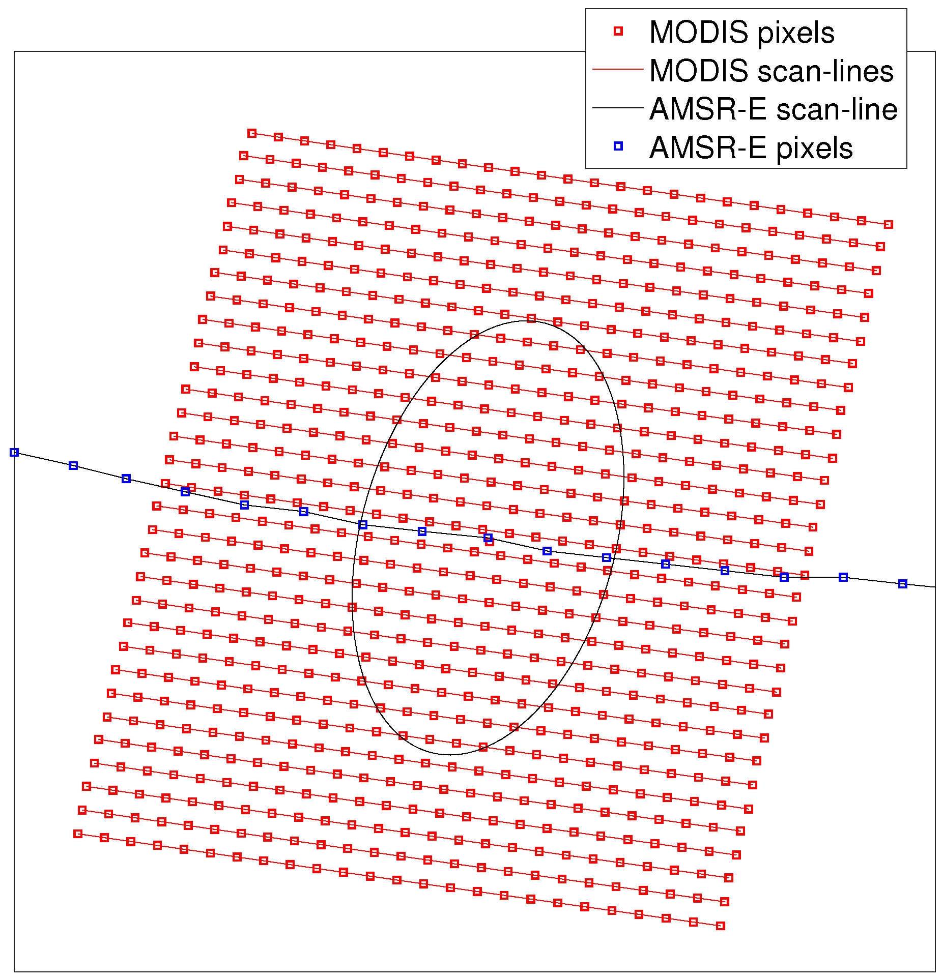
The starting point for this work was an approximately four million point AMSR-E–MODIS SST matchup dataset generated as part of this analysis as follows. A matchup was defined as a nighttime L2 AMSR-E SST pixel, meeting the quality criteria specified in Section 2.1, and a 101×125 MODIS L2 SST pixel region, centered on the AMSR-E pixel, for which 90% of the MODIS pixels were classified as clear—quality 0. The 101 element dimension of the MODIS regions selected is defined parallel to the MODIS across-track direction. The 125 element dimension was in the along-track direction. The size of the MODIS region was selected so that it would include all pixels contributing to the radiances of all bands used to determine the AMSR-E SST. As noted in Section 2.1, the AMSR-E antenna scanned at an off-nadir angle (47.5 from nadir) with each scan line defining an approximately circular section (Figure 1). Samples, numbered from −121 to 121, with zero corresponding to the scan center, were taken approximately every 10 km along this circular section as shown in Figure 2.
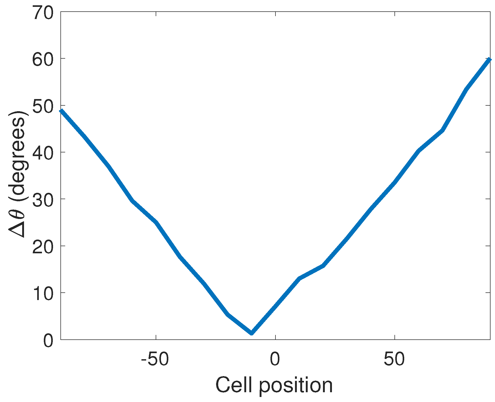
Important for this discussion, the semi-major axes of the footprints of the AMSR-E spectral bands (AMSR-E spectral footprints hereafter) were parallel to the vector from the nadir position of the satellite to the pixel of interest. By contrast, MODIS scanned along lines passing through nadir, lines that were approximately normal to the nadir track. This resulted in an angle, which depended on cell position, between the semi-major axis of the AMSR-E spectral footprints and the MODIS scan geometry. Figure 3 shows this angle at each cell position. The approximately 50 km offset of the cell at which the AMSR-E scan-line is parallel to the MODIS scan-line results from the Earth’s rotation. The AMSR-E and MODIS scans were centered on the direction in which the satellite is flying and the across-track direction of the scans were nearly perpendicular to the orbit of the satellite. This means that lines normal to the scans at their centers made an approximately 3.5 angle relative to the nadir track because the Earth is rotating under the satellite’s orbit. The AMSR-E scan at the Earth’s surface was approximately 870 km from the satellite’s nadir point so, the MODIS scan at the location at which the AMSR-E scan intersects the nadir track is made approximately 130 s after the AMSR-E scan. In that time, the Earth rotated approximately 50 km westward at the Equator.
Note that a matchup could also have been defined with one of the axes perpendicular to the AMSR-E scan line at the pixel of interest, however, this would have entailed a more complex subsampling of the MODIS data. Furthermore, it was not known at the outset whether or not the AMSR-E SST footprint would be aligned with the AMSR-E spectral footprints.
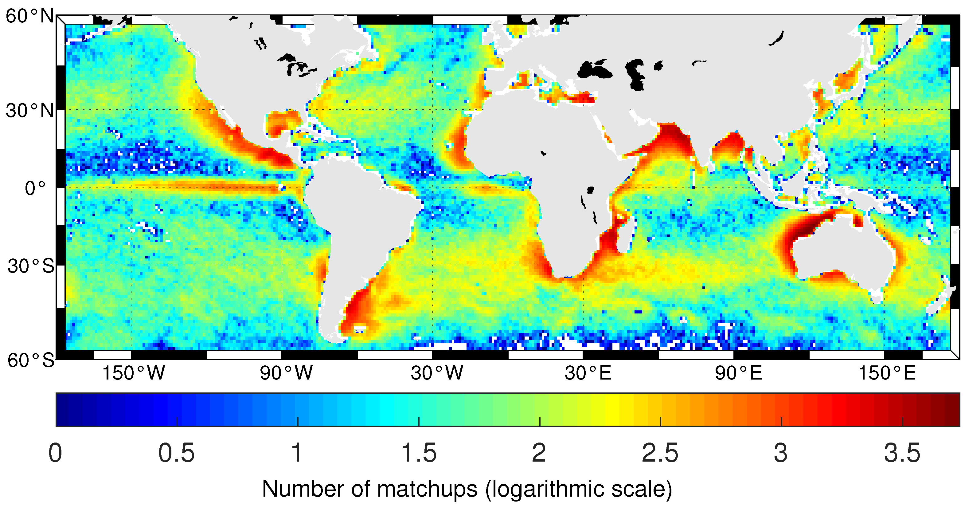
Gaps, if they exist in the MODIS patch, were filled by solving the Laplace equation with Dirichlet boundary conditions using the MATLAB routine roifill. Following this step, the full resolution MODIS data were degraded to lower resolution (for computational efficiency, as will be shown in Section 3.2) by averaging the initial fields over 4 × 4 pixels (≈4 km resolution at nadir). This resulted in a total of 775 (25 × 31) MODIS SST measurements. Figure 4 shows the global distribution of the matchup data. This figure is plotted with a logarithmic scale because of the variability in the number of samples from one region to another, with coastal areas tending to be much more clear than most of the open ocean.
Finally, the matchup dataset also contains additional information about the AMSR-E SST pixel: cell position, longitude coordinates and the retrieval time, allowing for stratification of the results based on these parameters.
3.2. Footprint Estimation Approach
To determine the AMSR-E SST footprint, we adopt a linear least-square method as described below, although other methods [18] may also be used. The method exploits the availability of cloud-free high-resolution MODIS SST data, considered as the true sub-resolution SSTs, that overlap each AMSR-E measurement. Consider an AMSR-E SST pixel as shown in Figure 2. The 25 × 31, 4 × 4 pixel averages of the original MODIS L2 SST field centered on the AMSR-E field-of-view, are displayed as red squares in the figure and the theoretical field-of-view of the AMSR-E channel is plotted in black. We express the MODIS pixels as a column vector . We express the AMSR-E pixels also as a column vector , where N is the number of matchu-ps used in the analysis. In perfect conditions (absence of measurement noises), the coarse-resolution AMSR-E SST measurement results from a weighted average of the sub-resolution SSTs (approximated here by the MODIS measurements). In this ideal case, the relation between the collection of all available AMSR-E SST pixel measurements (A) and MODIS mach-ups (M), can be written as:
or more compactly as:
where H is the footprint vector containing the weighting elements. A more realistic representation, i.e., one including measurement noise , can be written as:
Equation (3) simply identifies a regression relation between A and M; i.e., the SST of every AMSR-E pixel is seen to be the H-weighted average of the sub-resolution MODIS SSTs. The problem of deriving the AMSR-E footprint is then equivalent to determining the correct form of H, which minimizes the following difference:
This is the standard linear least-square problem, and there are several methods [19] for solving this type of problem. However, the solution to this problem allows for both positive and negative values of the elements of H, but it is unlikely that any of the regions in the AMSR-E field-of-view have a negative weight, this would be equivalent to a negative number of photons arriving at the detector from the region. We therefore add the constraint that all elements of H must be positive:
In addition, assuming that there is no bias between the AMSR-E field and the MODIS field, the elements of H should sum to one to preserve the mean value of the AMSR-E SST pixel—the temperature of an AMSR-E SST retrieval from a uniform field should be the temperature of the field. To facilitate the analysis, we fold any bias between the retrievals into the error term of Equation (3) and apply the following constraint:
Subject to these constraints our least squares problem becomes:
We used the Matlab solver, lsqlin, to determine H subject to the given constraints and the known values A (AMSR-E SST pixels) and M (the corresponding MODIS pixels). As previously noted, the infrared MODIS SST data are used as a proxy for the ground truth. Given that real observations are being used for the ‘ground truth’, they will include measurement errors, hence they are not quite the ‘truth’. However, as long as the errors of the MODIS SST values are randomly distributed from matchup to matchup, they will only increase the term in Equation (3). Specifically, the MODIS SST measurement model for the machup data used here can be expressed as:
where are the true values of SST and is the measurement noise associated with individual MODIS pixels. The weighted average of these values contribute to through the term. This term includes contributions from the retrieval algorithm, noise in the sensor and misclassification of cloud-contaminated pixels. It also includes any geophysical differences between AMSR-E SSTs and MODIS SSTs resulting from the fact that they are sampling over slightly different depth ranges; the upper 1 mm for the microwave retrievals and the upper m for the infrared retrievals. Given that there is no reason to expect any of these errors to have a preferred location in the AMSR-E footprint, the only effect of MODIS errors or of the slight differences in the geophysical variable being measured is to increase the noise term in Equation (2) with a concomitant increase in the uncertainty of the estimated footprints.
Because measurement noise and errors are unavoidable in practice, we adopt the uniform subsampling bootstrap procedure [20] to solve Equation (7). Let (, ), (, ),⋯, (, ) be sets of samples obtained from (, ) with . The elements of each set are drawn uniformly and independently, without replacement, from . For each of the bootstrap samples, we solved Equation (7) using the reduced matchup dataset. The resulting footprint was then obtained by averaging the individual bootstrap solutions. The following Algorithm 1 illustrates the scheme.
| Algorithm 1 Advanced microwave scanning radiometer-Earth observing satellite (EOS) (AMSR-E) footprint algorithm. |
|
4. Results
4.1. Simulation Study
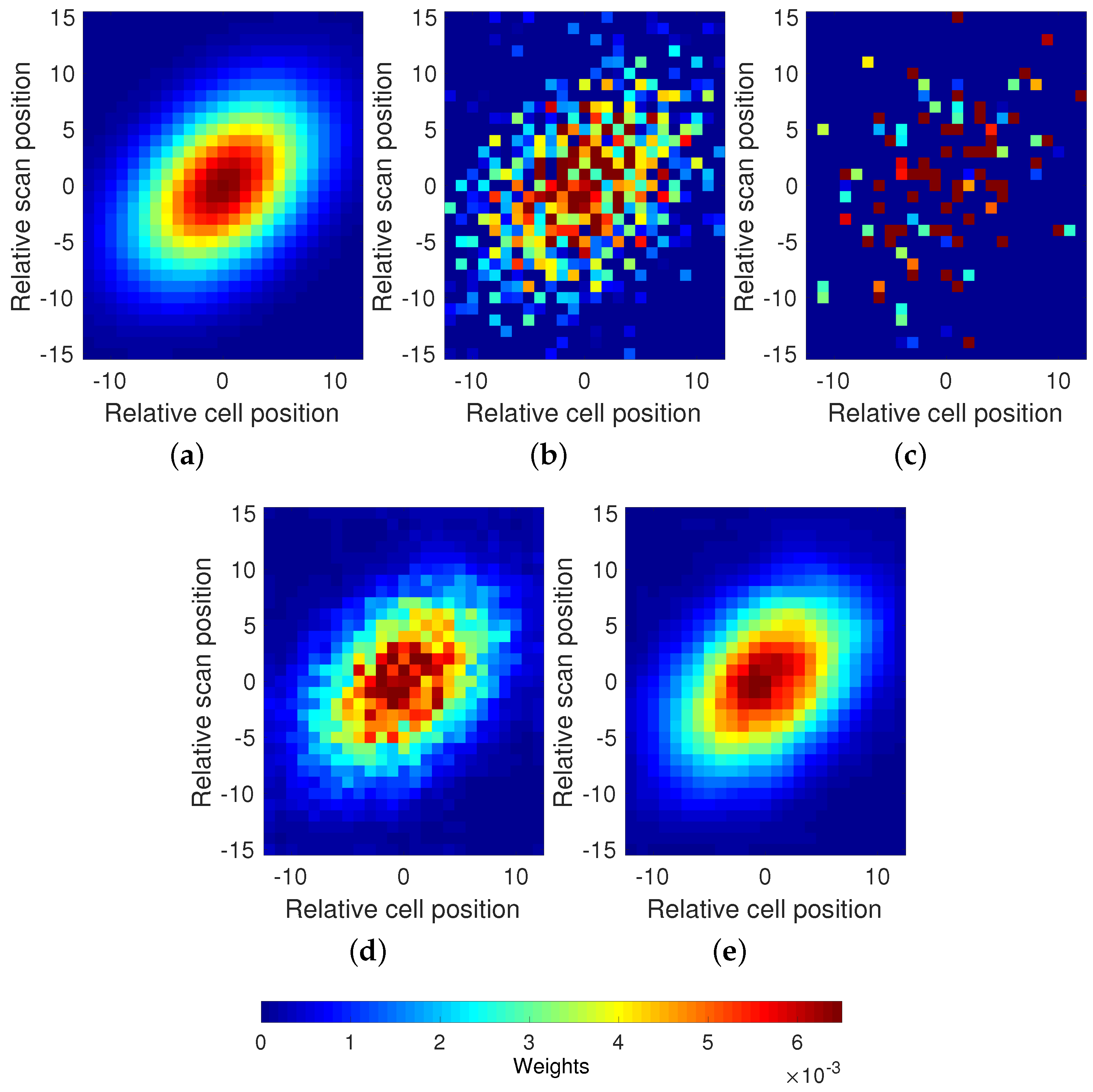
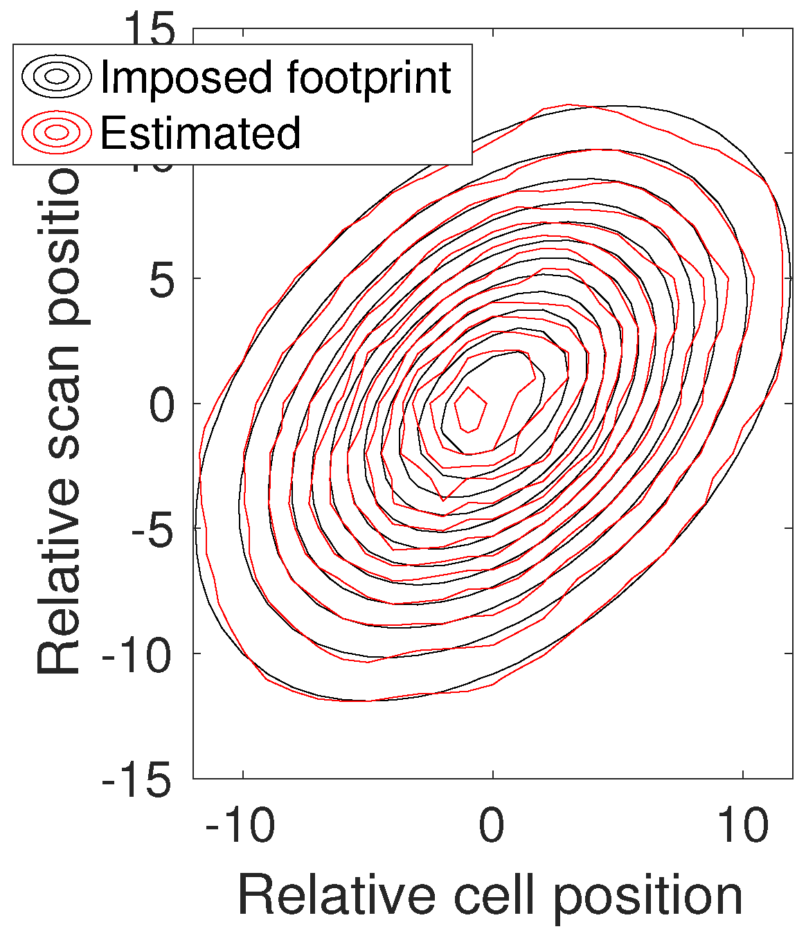
Simulations were undertaken to analyze the performance of the estimation algorithm. The results of these simulations were used to choose R, the number of bootstrap samples, and n, the number of matchu-ps in each sample, when the algorithm was applied to the actual dataset. A simple (but realistic) AMSR-E footprint (referred to as the imposed footprint hereafter) was used to generate simulated microwave measurements from 250,000 real high-resolution MODIS patches according to Equation (3). The 250,000 patches were randomly selected from the approximately four million matchu-ps discussed in Section 3.1, with the actual AMSR-E values being replaced by simulated values. For the imposed footprint, we used an elliptical Gaussian function with its major axis rotated 45 clockwise, about the vertical-axis with an aspect ratio of 1.74 (≈75/43) approximating the aspect ratio of the AMSR-E channel. The footprint is normalized according to Equations (5) and (6). Microwave measurements were simulated with Equation (3), using MODIS data as the ground truth, to which we added Gaussian white noise with a standard-deviation of 0.2 K. 0.05 K Gaussian white noise was added to the MODIS data in order to simulate the infrared instrument noise; i.e., the original MODIS field was taken as the true SST field and the simulated AMSR-E and MODIS fields were obtained from the ‘true’ field. The footprint was then estimated using the method described in Section 3.2. Footprints were retrieved for three different sets of parameters = (1; 250,000), (1; 2000), (2000; 2000). Figure 5a shows the imposed footprint, which we aim to reconstruct, used to generate the AMSR-E samples from the MODIS data. The retrieved footprints without bootstrap sampling (i.e., ; Figure 5b,c) were dominated by noise. The results of regularization (bootstrapping procedure; Figure 5d), showed a dramatic decrease in the noise of the retrieved footprint with the rotated Gaussian shape of the imposed footprint emerging clearly. Smoothing the retrieved footprint with a moving average further reduced the noise yielding a close facsimile to the imposed footprint (Figure 5e and Figure 6).
4.2. AMSR-E Footprint Estimation
In this section we examine the retrieved AMSR-E SST footprint (the SST footprint henceforth to distinguish it from the footprint of individual spectral bands), as a function of AMSR-E cell position, latitude and year. Because the relative angle between the local MODIS coordinate axis and the orientation of the AMSR-E spectral footprint varies with cell position (Figure 3), the orientation of the SST footprint depends on cell position; hence the decision to retrieve the SST footprint as a function of cell position. A latitudinal dependence could arise from a dependence on the target temperature or on orbital position. Finally, we examined the temporal dependence over the life of the sensor to determine whether or not the footprint changed with time. Recall that SST was determined from a combination of spectral channels and of polarizations for each channel and changes in any of the other channels and/or changes in the characteristics of the other retrieved parameters could impact the SST retrievals.
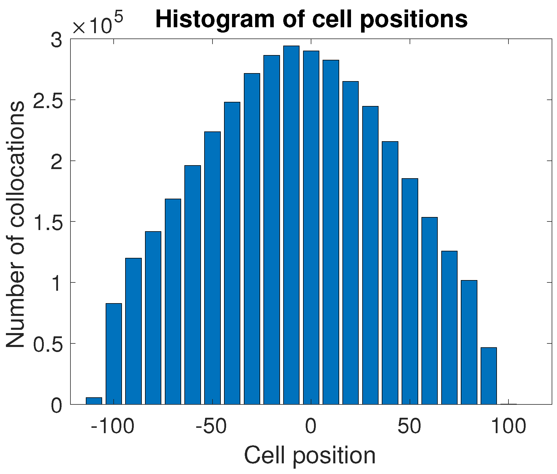
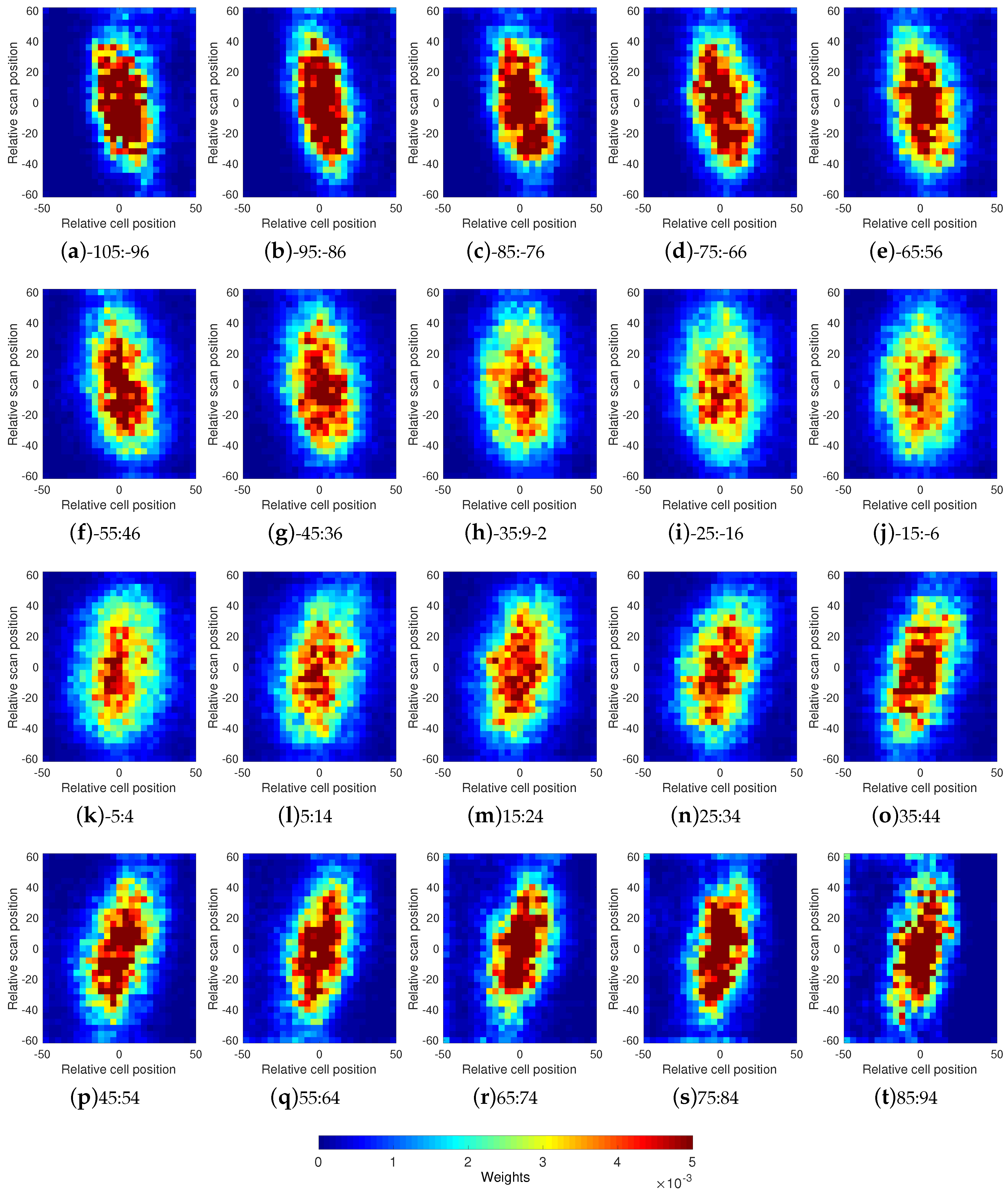
Cell position dependence. Matchups were binned by cell position (relative to nadir), with each bin containing a ten position range starting with cell position −115 (−115 to −106, −105 to −96, …, 85 to 94). Samples near the edge of the swath were not included in the analysis as they do not meet the quality criteria specified in Section 2; hence cell position −115 (as opposed to −122) was used as the starting cell position and cell position 96 (as opposed to 122) as the ending number. The reason that the binning was not centered on cell position 0, which corresponds to nadir, is because the angle between the MODIS and AMSR-E scans occurred at cell position 10, not 0; i.e., because the rotation axis of the antenna pointed slightly off nadir. Binning by ten cell positions provided a suitable number of matchups while adequately capturing any cross-track dependence (Figure 7).
In Figure 8, we show the empirically derived footprints for each cell position bin. The algorithm characterized by Equation (7), with (number of bootstrap repetitions) and (sample size), was applied to the matchup datasets associated with each cell position bin. Only bins involving more than 40,000 matchups were considered (20 bins). The retrieved footprints all suggest a basic elliptical shape but they differed in two key ways. Firstly, the orientation of the ellipses changed with respect to the cell position. Secondly, as the distance from nadir increases, the AMSR-E footprint becomes narrower in the across-track direction with a concomitant increase in intensity—recall that the weighting function must sum to 1.0 (Equation (7)) so the increase in intensity is consistent with the narrowing of the footprint. The varying rotation of angles results from two factors. First, the non-alignment of scan lines of the two sensors shown in Figure 3. Second, the axes of the plots in Figure 8 are in MODIS pixels, not in kilometers. Because the separation of MODIS pixels in the across-track direction increases with distance from nadir, the length of the horizontal axes increase. In contrast, the separation of MODIS pixels in the along-track direction changes little with distance from nadir, so the length of the vertical axes remain approximately the same from one end of the AMSR-E scan line to the other. The net effect of this is to decrease the magnitude of the apparent angles of the ellipse. The increase in intensity with distance from nadir results from the concomitant increase in the across-track spacing and in the size of MODIS pixels. The pixel intensity of the retrieved footprint at a given location is determined by the contribution of the sub-resolution MODIS SST element to the AMSR-E SST at the same location. Consequently, the larger the pixel size the more intense the contribution. Reassuringly, the footprints do not show a significant change in size in the along-track direction.
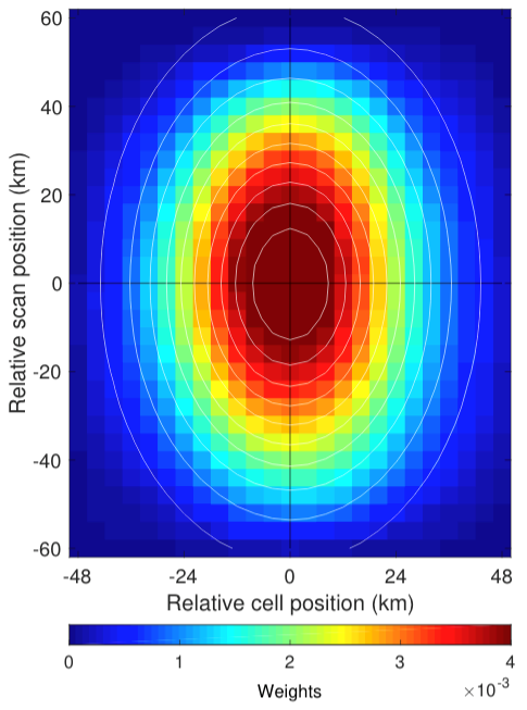
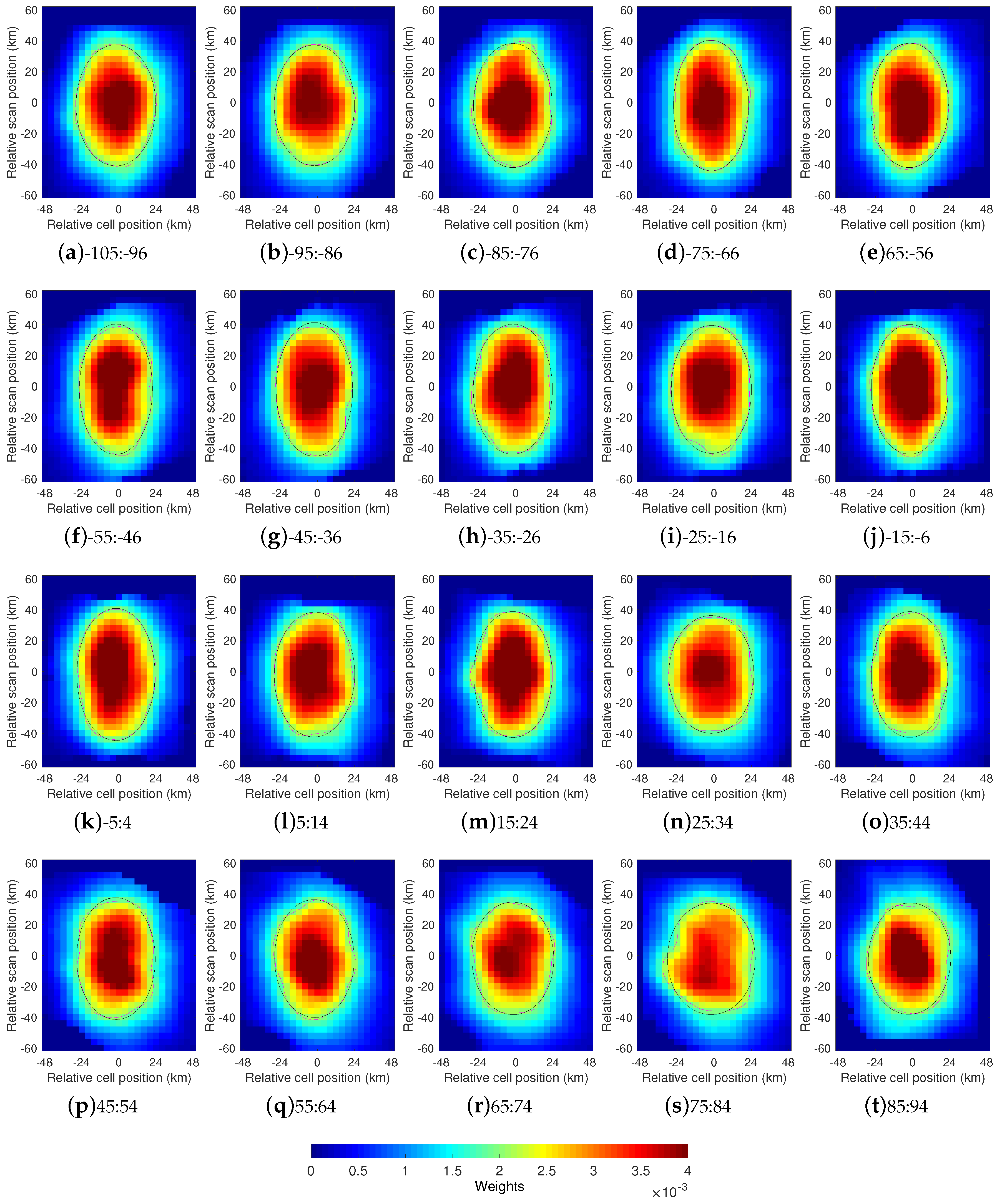
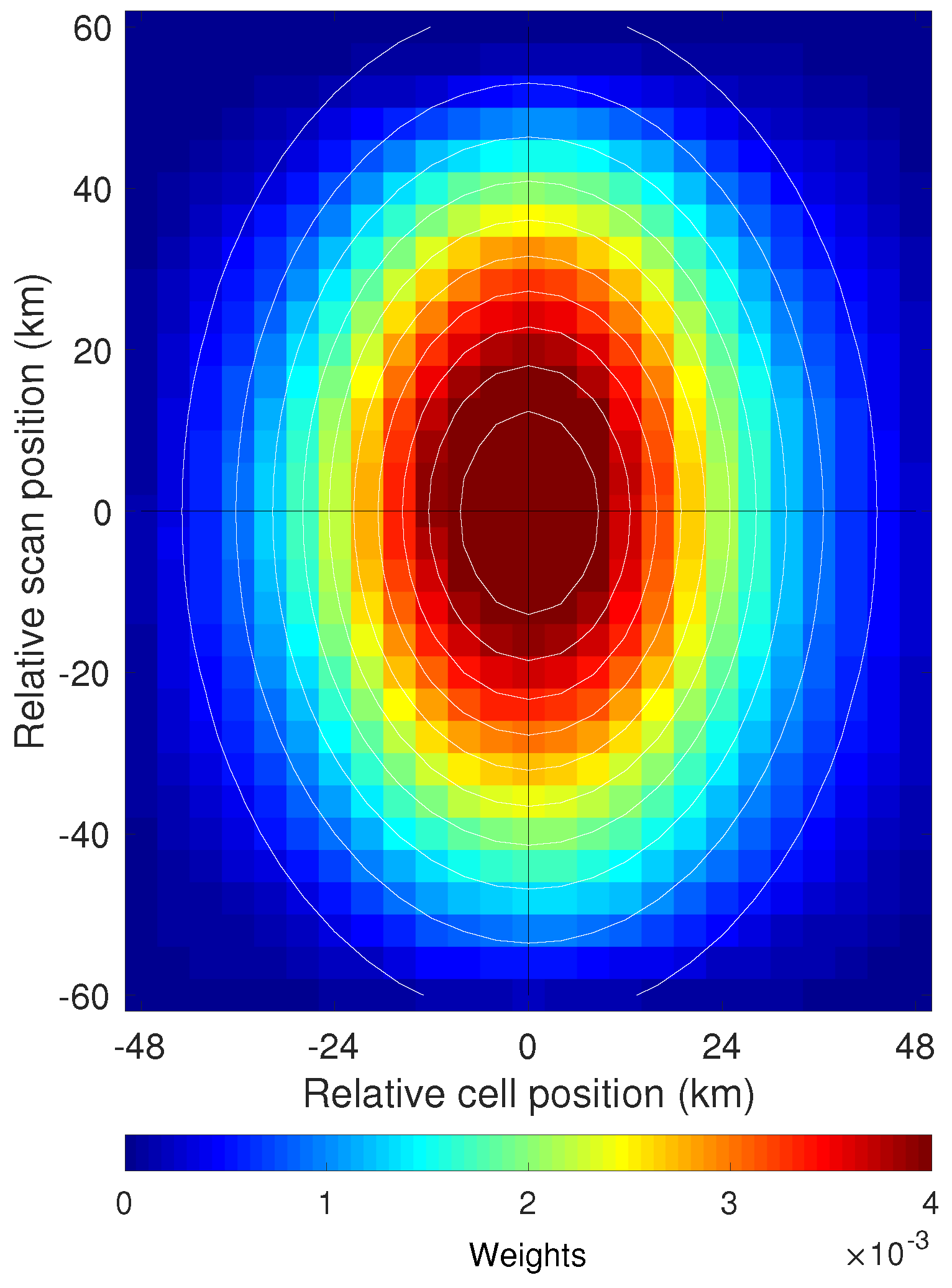
In the previous paragraph, we found that the retrieved footprint depended on the AMSR-E cell position and on the size of MODIS pixels. In order to remove these dependencies, so that the across-track footprint properties can be better studied and a mean footprint derived, the following correction procedure was undertaken. First, we applied a pixel moving average to the across-track footprints (Figure 8) in order to reduce the pixel-to-pixel noise. We then used the Matlab griddata function to transform the MODIS grid (with the x-axis parallel to scan lines, the y-axis parallel to the nadir track and grid spacing in pixels), in which the footprints are produced, to a Euclidean grid in kilometers, aligned with the instantaneous AMSR-E field of view. The results of this procedure are shown in Figure 9. The transformations applied have clearly removed the cell position dependence of the retrieved footprints, with all of the footprints now generally similar. This is not surprising given that the angle between nadir and the direction to the AMSR-E samples is very nearly independent of cell position. The similarity of the retrieved footprints suggests that a more accurate canonical footprint can be obtained by averaging the footprints of Figure 9. Figure 10 presents this average. A significant improvement was observed—the elliptical shape was considerably clearer and much smoother in comparison with the individual footprints. The standard error of the mean of the weights does not exceed ; the mean of these values over the entire footprint is , well below estimated weights on the outer edge of the footprint. In what follows, the across-track averaged footprint, f, is considered as the reference AMSR-E SST footprint to be used for the latitudinal and temporal analyses. This is also the footprint that we recommend using in other studies requiring knowledge of the characteristics of the AMSR-E SST footprint. (The change in notation from H used to represent the footprint in Equations (2)–(7) to f used in Equations (9)–(10), reflects the change from the footprint in satellite coordinates to the footprint in cartesian coordinates discussed above.) To facilitate quantitative comparisons, we render the reference footprint in functional form. Specifically, a curve of the form:
has been fit, in a least squares sense, to the retrieved mean AMSR-E footprint (Figure 10). The best fit parameters are: , , , km and km. The fitted model is represented as white contour lines superimposed on the mean footprint in Figure 10. The parameter indicates that the semi-major axis of the retrieved footprint is normal to the local tangent to the AMSR-E scan line. The angles obtained when averaging over bins on one side or the other of the nadir track were not statistically different from either.
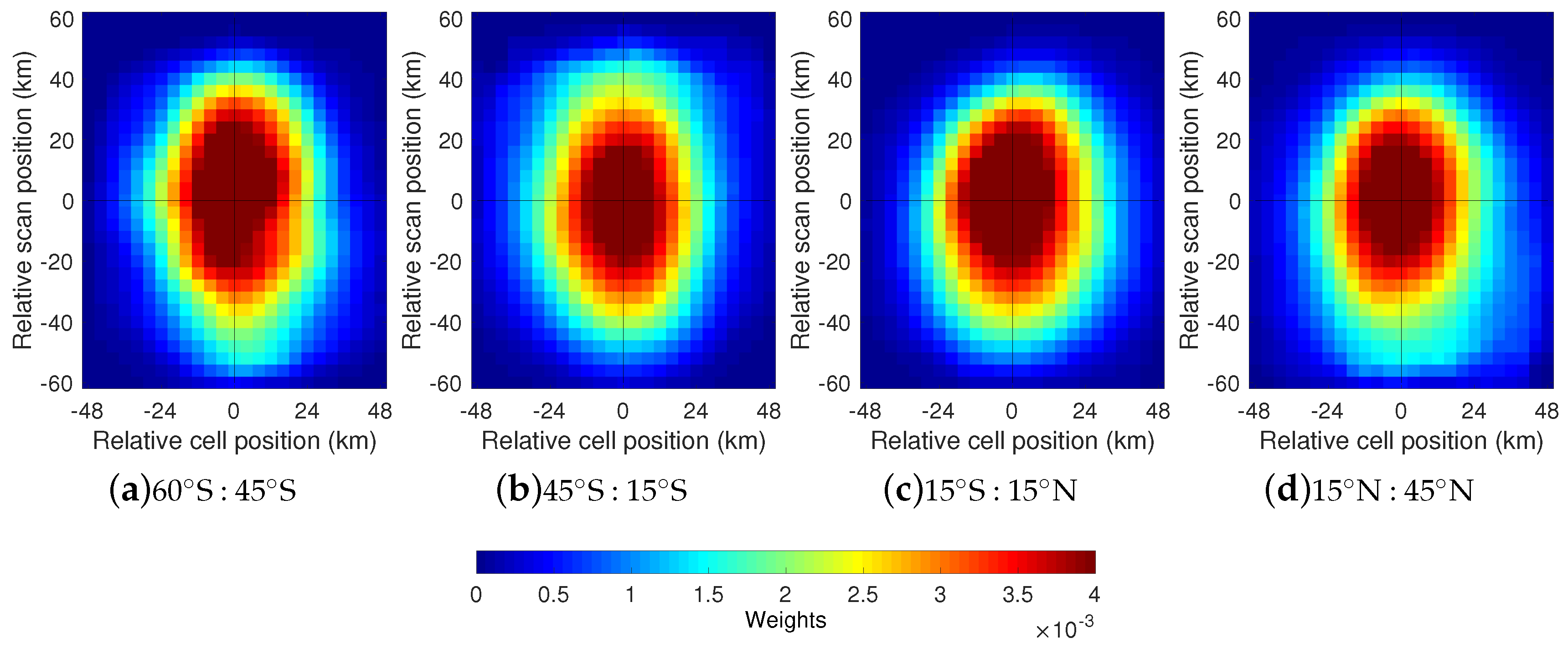
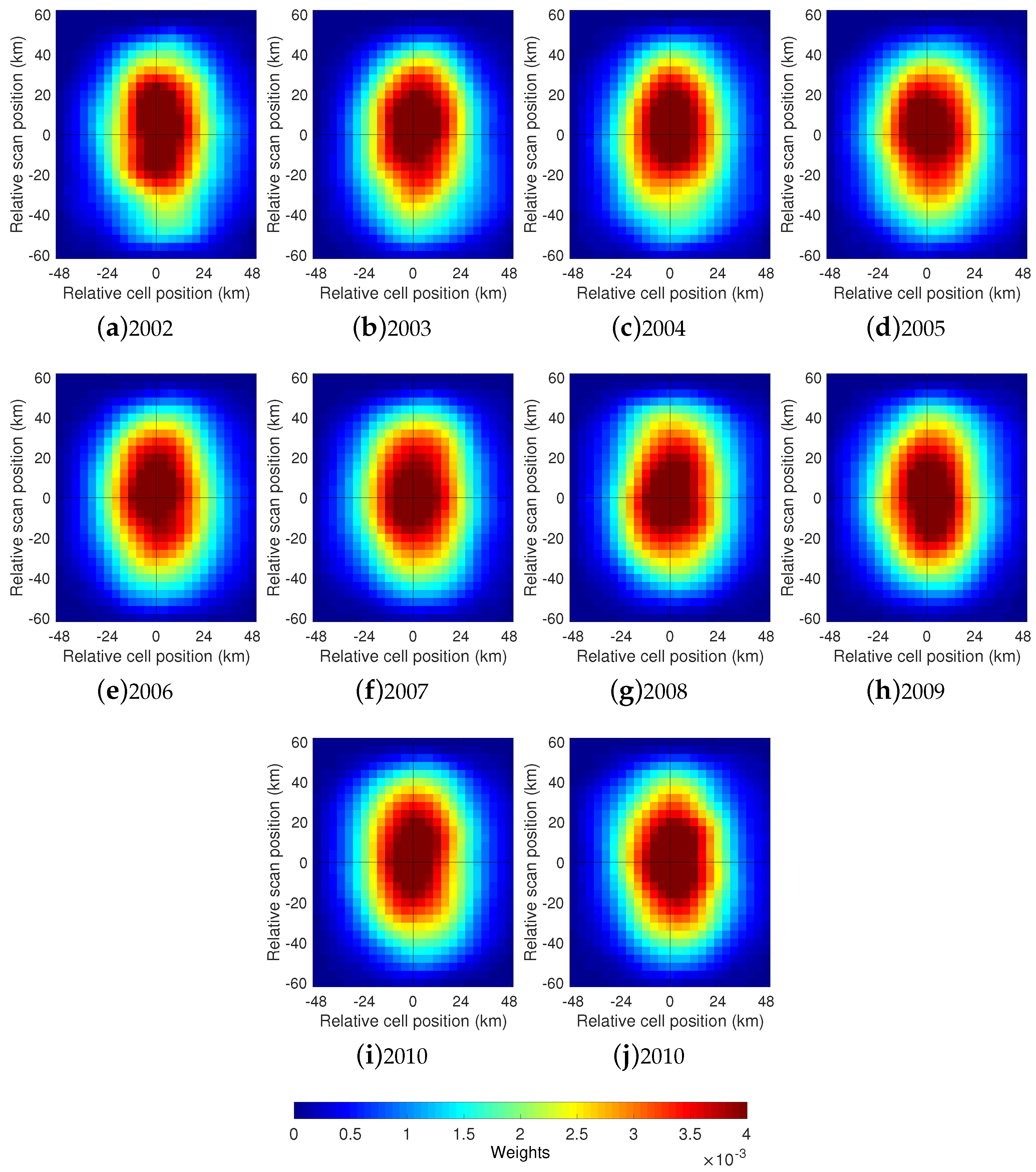
Latitudinal and temporal dependence. Each of the cell position bin matchup datasets was then binned into four latitudinal bands from S to N. For each of these bins, the across-track footprints were estimated using the procedure described above, normalized and averaged to obtain a footprint for the given latitudinal bin. The retrieved footprints are shown in Figure 11. Temporal analysis of the footprint was undertaken similarly, except that the cell position bin matchup datasets were binned by year for each year of the 10-year AMSR-E mission (2002 through 2011). The annual across-track averaged footprints are shown in Figure 12. The number of matchups used to derive the temporal and latitude-based footprints is, of course, reduced compared with number used to obtain the reference footprint, by approximately a factor of four in the latitudinal case and a factor of ten in the annual case, but the resulting footprints are still visually comparable to the reference footprint.
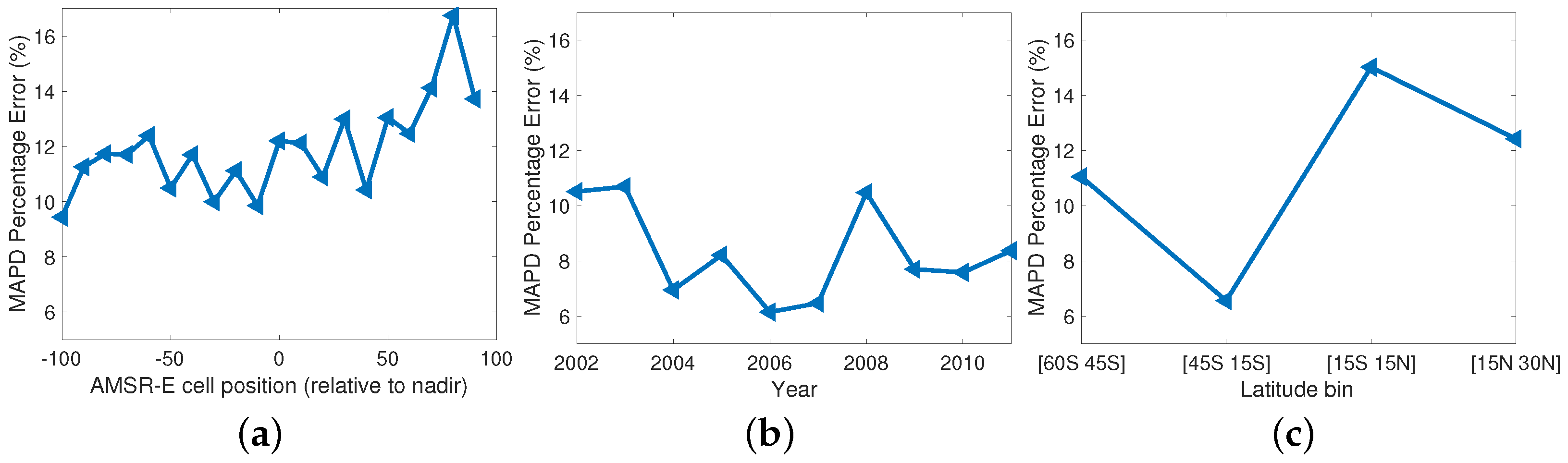
Statistical comparisons. In order to quantitatively compare the dependence of the footprint on cell position, latitude and year, we use two different statistics, one based on the mean absolute percentage deviation (MAPD), a measure of the deviation of a given footprint from a reference footprint as a percentage, and the other based on the aspect ratio of the best fit ellipse to the footprint, a measure of the deviation of a given footprint from a reference footprint based on shape. Both sets of statistics were determined for the footprints shown in Figure 9 (cell position), Figure 11 (latitude) and Figure 12 (year). We begin with the MAPD statistic, defined as follows:
where f is the footprint to evaluate (e.g., retrieved at a particular cell position) and is the reference footprint, depicted in Figure 10. (MAPD was chosen as one of the two statistics because of the ease in its interpretation. Possible issues with very small values contributing an outsized share to MAPD were reduced by excluding the border of the footprint, where the weights are very low, before its estimation.) The results are shown in Figure 13a for the across-track dependence, Figure 13b for annual dependence and Figure 13c for the latitudinal dependence. In all cases, the amplitude of the deviations is below . The deviations are found to be smaller for the year-by-year estimates. This was expected considering that the footprints correspond to an average over all the cell positions. The best yearly MAPD value is around 6% with an average of . The latitudinal footprints also result from across-track averaging but the associated deviations show more variability. This may be due to the variability in the SST fields; the smoother the field the larger the deviation of the retrieved footprint since the approach used here is not able to obtain an estimate of the footprint from a flat field. SST fields equatorward of 30 N/S tend to be more uniform that those in the subtropics. The across-track MAPD results tend to be relatively stable for negative cell positions and show an increasing trend with the increasing positive cell positions. The reason for this is not clear.
The second method for comparing footprints is based on the aspect ratio of the footprint determined as follows. For each estimated footprint, we extracted the contour-line (magenta curves in Figure 9 for the along-scan footprints). An ellipse was then least squares fitted to the extracted contour (black curves in Figure 9) and the aspect ratio, , of this ellipse was calculated, where is the length of the semi-major axis and that of the semi-minor axis. The 0.002 contour line used in these fits corresponds to one half of the maximum value of the mean footprint (half of the fitted value of a in Equation (9)). The same procedure, applied to the mean footprint (Figure 10), resulted in an aspect ratio of ; somewhat smaller than the 1.74 value of the AMSR-E bands. Figure 14 shows the aspect ratio by (a) cell position, (b) year and (c) latitude. The footprint was stable for the entire mission at approximately the value of the reference footprint. There also appears to be little latitudinal dependence. By contrast, the cell position plot shows a trend from one side of nadir to the other. This trend is not understood but it is likely related to the suggestion of an across-track trend in MAPD discussed in the previous paragraph.
5. Discussion
The reference footprint, obtained by averaging the retrievals across all cell positions, is close to the shape and size of the pixel, this despite the inclusion of data from other spectral bands and additional processing. This came as somewhat of a surprise to us because we had understood that the SST values retrieved from the re-gridded brightness temperatures were averaged over five AMSR-E pixels in the across-scan direction, hence we expected that the SST footprint would be approximately 20 km larger in the direction normal to the scan line. This does not appear to be the case.
The average footprint obtained in this study is robust through time as well as a function of latitude, suggesting that it is a good first choice for the SST footprint where the shape and size of the footprint is relevant.
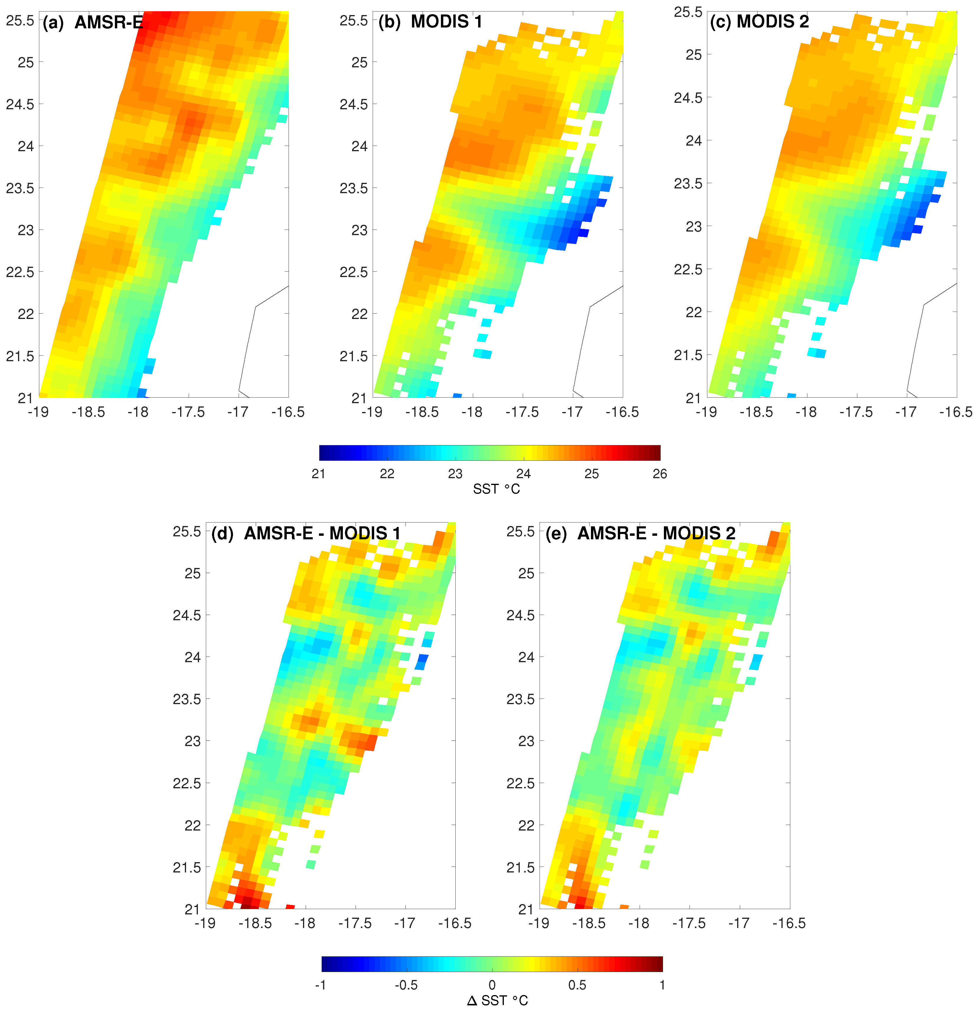
In order to demonstrate the importance of properly representing the AMSR-E SST footprint, we compare the AMSR-E SST field of 0155 UCT, 2009-10-31 minus the coincident MODIS SST field, assuming a km AMSR-E footprint, with the same difference, assuming the footprint represented by Figure 10. The criteria used to select the field was that it be largely cloud free and that there be some structure in it—the shape of the footprint is irrelevant when comparing retrievals from different sensors for a uniform field. To difference the fields, it is necessary to map them to the same grid. In this case, the MODIS data were mapped to the AMSR-E field. Specifically, for each AMSR-E pixel, all L2 MODIS SST values falling within the “footprint” of the AMSR-E pixel were averaged. The AMSR-E field is shown in Figure 15a. The MODIS field, averaged to the AMSR-E field using the km square footprint, is shown in Figure 15b and the MODIS field, averaged to the AMSR-E field using the footprint of Figure 10 is shown in Figure 15c. The difference field for the km footprint is shown in Figure 15d and that for the footprint of Figure 10 is shown in Figure 15e. The difference field associated with the 56 km footprint shows structure not in that associated with the footprint of Figure 10.
Finally, although we obtained the AMSR-E SST footprint through use of the very nearly simultaneous MODIS SST product, we do not believe that the simultaneity of the observations is critical. One could use SST products from other high resolution infrared sensors as long as the time separating the observations is less than six hours. The important consideration here is to avoid times when the surface temperature is changing rapidly, specifically during daylight hours hence the six hour constraint. There must, of course, also be a large number of matchups with whatever sensor is being used to obtain the footprint.
6. Conclusions
The constraint least square method has been applied to a large AMSR-E-MODIS matchup dataset to estimate the footprint (the weights of sub-resolution pixels within a given pixel) of the L2 AMSR-E SST product produced by Remote Sensing Systems. This was done based on the higher resolution L2 MODIS SST dataset (coincident in space and time with the AMSR-E dataset) produced by NASA’s Ocean Biology Processing Group. Bootstrapping (bagging) was used to reduce the noise of the retrieved footprint.
The analysis was undertaken as a function of the AMSR-E cell position. The footprint orientation with regard to the nadir track and the apparent size of the footprint was found to vary with distance from nadir. This was due to the angle between the local tangent to the AMSR-E scan-line and to the size of the MODIS pixel, both of which increase away from nadir. Once recast into a coordinate system with axes parallel and normal to the local tangent, the across-track footprint was shown to be independent of cell position and the resulting footprints were averaged to obtain a reference footprint, an elliptic Gaussian-like kernel with an aspect ratio of 1.58. This aspect ratio is close to the that of the AMSR-E 6.93 GHz channel, 1.74.
Temporal and latitudinal analyses were also undertaken and the footprint was found to be independent of these parameters as well.
These results suggest that careful application of the reference footprint when comparing datasets should result in a reduction of root mean square differences over the use of the often quoted 56 × 56 km AMSR-E SST footprint. The reference footprint is also the appropriate footprint to use in the deconvolution of the heavily oversampled AMSR-E SST dataset.
Finally, as we note above, these results apply only to the RSS L2 SST product. However, the same approach could be used to determine the SST footprint of other, including uncollated L3, products. Furthermore, the stability of the footprint over time is likely to prove true for other products as well since this depends primarily on the geometry of the instrument as it relates to the satellite.
7. Data Availability
The reference footprint determined in this study is publicly available at the Harvard Dataverse Network https://dataverse.harvard.edu/dataset.xhtml?persistentId=doi:10.7910/DVN/H2PHP0.
Author Contributions
B.B. performed the analysis and wrote the original draft of the manuscript. P.C. contributed significantly to the writing of the manuscript. B.B., P.C. and G.P. conceived the study and all contributed to the theoretical aspects of the analysis. C.G. provided support related to the details of AMSR-E and the processing of AMSR-E brightness temperatures to SST.
Funding
This research was funded by the NASA Physical Oceanography Program (Grant #NNX16AI24G) and as part of NOPP funding (80NSSC18K0837). Partial salary support for P. Cornillon was provided by the State of Rhode Island and Providence Plantations.
Acknowledgments
AMSR-E data were produced by remote sensing systems (RSS) and sponsored by the NASA AMSR-E Science Team. Data were acquired from the PO-DAAC server at: https://podaac.jpl.nasa.gov. MODIS data were produced by the NASA’s Ocean Biology Processing Group and acquired from: http://oceancolor.gsfc.nasa.gov. The authors gratefully acknowledge the use of the High Performance Research Computing facility provided by the University of Rhode Island.
Conflicts of Interest
The authors declare no conflict of interest.
Abbreviations
The following abbreviations are used in this manuscript:
| AMSR-E | Advanced microwave scanning radiometer-EOS |
| ECV | Essential climate variable |
| JAXA | Japan Aerospace Exploration Agency |
| MAPD | Mean absolute percentage deviation |
| MODIS | Moderate-resolution imaging spectroradiometer |
| NASA | National Aeronautics and Space Administration |
| NASDA | National Space Development Agency (Japan) |
| OBPG | Ocean Biology Processing Group |
| PO-DAAC | Physical Oceanography-Distributed Active Archive Center |
| RFI | Radio frequency interference |
| RSS | Remote sensing systems |
| SST | Sea surface temperature |
| WS | Wind speed |
References
- GCOS. Systematic Observation Requirements for Satellite-Based Products for Climate-Supplemental Details to the Satellite-Based Component of the “Implementation Plan for the Global Observing System for Climate in Support of the UNFCCC”; Technical Report GCOS-107, WMO/TD No 1338; WMO: Geneva, Switzerland, 2006. [Google Scholar]
- Chelton, D.B.; Wentz, F.J. Global Microwave Satellite Observations of Sea Surface Temperature for Numerical Weather Prediction and Climate Research. Bull. Am. Meteorol. Soc. 2005, 86, 1097–1116. [Google Scholar] [CrossRef] [Green Version]
- Parkinson, C.L. Aqua: An Earth-observing satellite mission to examine water and other climate variables. IEEE Trans. Geosci. Remote Sens. 2003, 41, 173–183. [Google Scholar] [CrossRef]
- O’Carroll, A.G.; Eyre, J.R.; Saunders, R.W. Three-Way Error Analysis between AATSR, AMSR-E, and In Situ Sea Surface Temperature Observations. J. Atmos. Ocean. Technol. 2008, 25, 1197–1207. [Google Scholar] [CrossRef] [Green Version]
- Lean, K.; Saunders, R.W. Validation of the ATSR Reprocessing for Climate (ARC) Dataset Using Data from Drifting Buoys and a Three-Way Error Analysis. J. Clim. 2013, 26, 4758–4772. [Google Scholar] [CrossRef]
- Gentemann, C.L. Three way validation of MODIS and AMSR-E sea surface temperatures. J. Geophys. Res. 2014, 119, 2583–2598. [Google Scholar] [CrossRef] [Green Version]
- Deschamps, P.Y.; Frouin, R.; CréPon, M. Sea surface temperatures of the coastal zones of France observed by the HCMM satellite. J. Geophys. Res. 1984, 89, 8123–8149. [Google Scholar] [CrossRef]
- Callies, J.; Ferrari, R. Interpreting Energy and Tracer Spectra of Upper-Ocean Turbulence in the Submesoscale Range (1–200 km). J. Phys. Oceanogr. 2013, 43, 2456–2474. [Google Scholar] [CrossRef] [Green Version]
- Gambardella, A.; Migliaccio, M. On the superresolution of microwave scanning radiometer measurements. IEEE Geosci. Remote Sens. Lett. 2008, 5, 796–800. [Google Scholar] [CrossRef]
- Wentz, F.J.; Gentemann, C.; Smith, D.; Chelton, D. Satellite Measurements of Sea Surface Temperature Through Clouds. Science 2000, 288, 847–850. [Google Scholar] [CrossRef] [PubMed]
- JAXA. AMSR-E Data Users Handbook; Japan Aerospace Exploration Agency: Hiki-Gun Saitama, Japan, 2006. Available online: https://www.eorc.jaxa.jp/en/hatoyama/amsr-e/amsr-e_handbook_e.pdf (accessed on 8 March 2017).
- Meyer-Lerbs, L. Gridding of AMSR-E Satellite Data. Master’s Thesis, University of Bremen, Bremen, Germany, 2005. Available online: http://www.iup.uni-bremen.de/PEP_master_thesis/thesis_2005/Thesis_LotharMeyer-Lerbs.pdf (accessed on 8 March 2017).
- Wentz, F.J.; Meissner, T. Supplement 1 Algorithm Theoretical Basis Document for AMSR-E Ocean Algorithms; NASA: Santa Rosa, CA, USA, 2007.
- Ocean Biology Processing Group, NASA Goddard Space Flight Center, Ocean Ecology Laboratory. Moderate-Resolution Imaging Spectroradiometer (MODIS) Aqua Sea Surface Temperature Data; 2014 Reprocessing; 2014. [CrossRef]
- Walton, C.C. Nonlinear multichannel algorithms for estimating sea surface temperature with AVHRR satellite data. J. Appl. Meteorol. 1988, 27, 115–124. [Google Scholar] [CrossRef]
- Franz, B. Implementation of SST Processing within the OBPG. Último Acceso 2006, 4, 2014. [Google Scholar]
- Wu, F.; Cornillon, P.; Boussidi, B.; Guan, L. Determining the Pixel-to-Pixel Uncertainty in Satellite-Derived SST Fields. Remote Sens. 2017, 9, 877. [Google Scholar] [CrossRef]
- Park, T.; Casella, G. The bayesian lasso. J. Am. Stat. Assoc. 2008, 103, 681–686. [Google Scholar] [CrossRef]
- Gill, P.E.; Murray, W.; Wright, M.H. Practical Optimization; Academic Press Inc.: London, UK, 1981. [Google Scholar]
- Bhattacharyya, S.; Bickel, P. Subsampling bootstrap of count features of networks. Ann. Stat. 2015, 43, 2384–2411. [Google Scholar] [CrossRef] [Green Version]
Figure 1.
The scan geometry of the Advanced Microwave Scanning Radiometer-Earth observing satellite (EOS) (AMSR-E). The ellipses schematically illustrate the AMSR-E footprint.
Figure 1.
The scan geometry of the Advanced Microwave Scanning Radiometer-Earth observing satellite (EOS) (AMSR-E). The ellipses schematically illustrate the AMSR-E footprint.

Figure 2.
Example of matchup data.

Figure 3.
Relative angle between AMSR-E and moderate-resolution imaging spectroradiometer (MODIS) scans as a function of AMSR-E cell position.
Figure 3.
Relative angle between AMSR-E and moderate-resolution imaging spectroradiometer (MODIS) scans as a function of AMSR-E cell position.

Figure 4.
Number of collocations. The distribution of collocations is a combination of where the MODIS and AMSR-E data are both present, and this is reflected by the higher number of collocations in clear sky region.
Figure 4.
Number of collocations. The distribution of collocations is a combination of where the MODIS and AMSR-E data are both present, and this is reflected by the higher number of collocations in clear sky region.

Figure 5.
The results using simulated AMSR-E measurements. (a) Imposed footprint; (b) Algorithm 1 output with = (1; 250,000); (c) and (d) ; (e) is achieved by applying a moving average to (d).
Figure 5.
The results using simulated AMSR-E measurements. (a) Imposed footprint; (b) Algorithm 1 output with = (1; 250,000); (c) and (d) ; (e) is achieved by applying a moving average to (d).

Figure 6.
The contour-lines of the imposed footprint (Figure 5a) and the final result shown in Figure 5e.

Figure 7.
Histogram of the cell positions for the matchups used in this paper.

Figure 8.
Estimated AMSR-E footprints determined from matchups over the AMSR-E cell range indicated in the sub-caption of each frame. The axes of each of the footprints are in units of MODIS pixels (no smoothing applied). First bin, −115 to −106, with relatively few matchups (Figure 7), is not shown.

Figure 9.
Estimated AMSR-E footprints obtained by projecting the footprints in Figure 8 on regular 4 km × 4 km grids aligned with the instantaneous AMSR-E field-of-view (a 4 × 4 moving averaged filter was applied prior the calculation). A contour-line at 0.002 level (magenta) and its best fitting ellipse (black) are traced for each footprint.

Figure 10.
AMSR-E footprint obtained by averaging the across-track footprints shown in Figure 9. Contour-lines of the fitted analytic model (Equation (9)) are superimposed and plotted in white color. The standard error of the mean of the weights does not exceed .

Figure 11.
Footprints representing across-track averages in four latitude bins.

Figure 12.
Year-by-year estimates of the across-track average footprints.

Figure 13.
MAPD Percentage deviation for (a) across-track, (b) year-by-year and (c) latitude-based footprint estimates.
Figure 13.
MAPD Percentage deviation for (a) across-track, (b) year-by-year and (c) latitude-based footprint estimates.

Figure 14.
The aspect ratio of the fitted ellipse to the 0.002 contour-line of the (a) across-track footprints shown in Figure 9, (b) year-by-year shown in Figure 12 and (c) those calculated as a function of latitude in Figure 11. The mean aspect ratio value corresponding to the ellipse fitted to the footprint shown in Figure 10 is plotted in red. The theoretical value corresponding to the channel aspect ratio is plotted in yellow (≈1.74).

Figure 15.
Comparison of (a) the AMSR-E SST field of 0155 UCT, 2009-10-31 with the coincident MODIS SST field assuming (b) a 56 × 56 km footprint, and (c) assuming the footprint represented by Figure 10. The AMSR-E SST field minus the two MODIS derived fields are, respectively, shown in (d,e).
Figure 15.
Comparison of (a) the AMSR-E SST field of 0155 UCT, 2009-10-31 with the coincident MODIS SST field assuming (b) a 56 × 56 km footprint, and (c) assuming the footprint represented by Figure 10. The AMSR-E SST field minus the two MODIS derived fields are, respectively, shown in (d,e).


Table 1.
Nominal footprint size (reproduced from ([11], pp. 2–31)).
Table 1.
Nominal footprint size (reproduced from ([11], pp. 2–31)).
| Frequency | Beam Width | Footprint |
|---|---|---|
| (GHz) | (, Nominal) | (km, Across-Track × Along-Track) |
| 6.925 | 2.2 | 43.2 × 75.4 |
| 10.65 | 1.5 | 29.4 × 51.4 |
| 18.7 | 0.8 | 15.7 × 27.4 |
| 23.8 | 0.9 | 18.1 × 31.5 |
| 36.5 | 0.4 | 8.2 × 14.4 |
| 89 | 0.2 | 3.7 × 6.5 |
| 89 | 0.2 | 3.5 × 5.9 |
© 2019 by the authors. Licensee MDPI, Basel, Switzerland. This article is an open access article distributed under the terms and conditions of the Creative Commons Attribution (CC BY) license (http://creativecommons.org/licenses/by/4.0/).
Share and Cite
MDPI and ACS Style
Boussidi, B.; Cornillon, P.; Puggioni, G.; Gentemann, C. Determining the AMSR-E SST Footprint from Co-Located MODIS SSTs. Remote Sens. 2019, 11, 715. https://0-doi-org.brum.beds.ac.uk/10.3390/rs11060715
AMA Style
Boussidi B, Cornillon P, Puggioni G, Gentemann C. Determining the AMSR-E SST Footprint from Co-Located MODIS SSTs. Remote Sensing. 2019; 11(6):715. https://0-doi-org.brum.beds.ac.uk/10.3390/rs11060715
Chicago/Turabian StyleBoussidi, Brahim, Peter Cornillon, Gavino Puggioni, and Chelle Gentemann. 2019. "Determining the AMSR-E SST Footprint from Co-Located MODIS SSTs" Remote Sensing 11, no. 6: 715. https://0-doi-org.brum.beds.ac.uk/10.3390/rs11060715
Note that from the first issue of 2016, this journal uses article numbers instead of page numbers. See further details here.