Article

Analysis of Retrackers’ Performances and Water Level Retrieval over the Ebro River Basin Using Sentinel-3

1
isardSAT, Parc Tecnològic Barcelona Activa, Carrer de Marie Curie 8, 08042 Barcelona, Catalonia, Spain
2
CESBIO (CNRS/CNES/UPS/IRD), 31401 CEDEX 9 Toulouse, France
3
Observatori de l’Ebre (OE), Ramon Llull University, 43520 Roquetes, Spain
*
Author to whom correspondence should be addressed.
Submission received: 29 January 2019 / Revised: 11 March 2019 / Accepted: 21 March 2019 / Published: 25 March 2019
(This article belongs to the Special Issue Advances in Satellite Altimetry and Its Application)

Abstract

:
Satellite altimeters have been used to monitor river and reservoir water levels, from which water storage estimates can be derived. Inland water altimetry can, therefore, play an important role in continental water resource management. Traditionally, satellite altimeters were designed to monitor homogeneous surfaces such as oceans or ice sheets, resulting in poor performance over small inland water bodies due to the contribution from land contamination in the returned waveforms. The advent of synthetic aperture radar (SAR) altimetry (with its improved along-track spatial resolution) has enabled the measurement of inland water levels with a better accuracy and an increased spatial resolution. This study aimed to retrieve water levels from Level-1B Sentinel-3 data with focus on the minimization of the land contamination over small- to middle-sized water bodies (130 m to 4.5 km), where continuous clean waveforms rarely exist. Three specialized algorithms or retrackers, together with a new waveform portion selection method, were evaluated to minimize land contamination in the waveforms and to select the nadir return associated with the water body being overflown. The waveform portion selection method, with consideration of the Digital Elevation Model (DEM), was used to fit the multipeak waveforms that arise when overflying the continental water bodies, exploiting a subwaveform-based approach to pick up the one corresponding to the nadir. The performances of the proposed waveform portion selection method with three retrackers, namely, the threshold retracker, Offset Center of Gravity (OCOG) retracker and two-step SAR physical-based retracker, were compared. No significant difference was found in the results of the three retrackers. However, waveform portion selection using DEM information great improved the results. Time series of water levels were retrieved for water bodies in the Ebro River basin (Spain). The results show good agreement with in situ measurements from the Ebro Reservoir (approximately 1.8 km wide) and Ribarroja Reservoir (approximately 400 m wide), with unbiased root-mean-square errors (RMSEs) down to 0.28 m and 0.16 m, respectively, depending on the retracker.

Graphical Abstract

1. Introduction

Inland water systems constitute crucial resources of fresh water necessary for human survival [1]. Water within rivers and reservoirs represent the primary supply of drinking water, agricultural irrigation and industrial water usage globally [2], and also used to produce renewable hydrological energy. In addition, floods that periodically occur in every region of the world represent threats to crops, settlements, infrastructure, and most importantly life. Therefore, it is important to monitor the water levels of inland water bodies to provide early-warning alerts for water shortages or flood predictions. Unfortunately, in situ gauging stations are not always available in many parts of the world, or not publicly available, being maintained by local authorities [3,4,5]. An alternative to this is the use of satellite radar altimeters. Satellite radar altimeters are essential tools for monitoring the oceans, a task they have performed for over 25 years [6]. Satellite radar altimetry has also proven to be valuable tools for monitoring the water levels within inland water systems, including lakes and rivers [3,7,8]. Satellite radar altimetry can help overcome the lack of data in many parts of the world, and contribute to monitoring the water levels both within inland water systems where no in situ data are available, and also within transboundary river basins.
A list of satellite radar altimetry missions and their resolutions is shown in Table 1. Until CryoSat-2 was launched, the satellite radar altimetry was pulse limited to low-resolution mode (LRM). CryoSat-2 is the first altimetry mission with the synthetic aperture radar (SAR) mode available, followed by Sentinel-3. Unlike classical pulse-limited altimetry, SAR altimetry exploits coherent processing of groups of transmitted pulses to make the most efficient use of the power reflected from the surface [9], therefore significantly improving along-track resolution [9,10,11], as shown in Table 1. Sentinel-3, the newest in-orbit satellite, has a temporal resolution of approximately 27 days and an inclination angle of approximately 98.6 degrees, meaning it can cover almost all Earth latitudes except the poles. Operating in high-resolution SAR mode [10], the ground track separation of Sentinel-3 at the equator is approximately 104 km. In contrast, the CryoSat-2 ground track separation at the equator reaches 7.7 km at the expense of its temporal resolution, at 369 days. Sentinel-3 exhibits the best along-track resolution at 300 m, close to the resolution of CryoSat-2 in SAR and interferometric SAR (SARIn) modes. However, CryoSat-2 has a focus on the cryosphere, and as a result covers most continental surfaces in LRM. Therefore, Sentinel-3 constitutes the first altimetry mission that covers the globe completely in SAR mode, and is thus the most ideal tool for inland water level monitoring thanks to its good global coverage and sufficient temporal and spatial resolutions.
The majority of previous studies [12,13,14,15,16,17,18,19,20,21,22,23,24,25,26,27] focus on relatively large water bodies with a scale of several kilometers. One of the first studies employing satellite altimetry for inland water level extraction was performed by Koblinsky et al. [12], who processed Geodetic Satellite (Geosat) waveforms to estimate the water levels at four sites in the Amazon basin. A root-mean-square error (RMSE) of 70 cm was estimated between the satellite and in situ measurements. Since then, with new generations of satellites, the spatial resolution and the accuracy of the orbit determination have both improved, thereby increasing the accuracies of the estimation results. Accordingly, several studies have since focused on lakes and large rivers with scales, ranging from 1000 km2 to 80,000 km2, and demonstrated good results [12,13,14,15,16,17,18,19,20,21,22,23,24,25,26,27]. For example, Nielsen et al. [17] used Environmental Satellite (Envisat) and CryoSat-2 SAR data to retrieve the water levels over Vaenern (Sweden, 5650 km2) and Lake Okeechobee (Florida, 1900 km2), and obtained good accuracies with RMSEs, varying from 4 cm to 9 cm between the satellite-retrieved water levels and in situ measurements. Currently, several online data hubs, such as the Database for Hydrological Time Series of Inland Waters (DAHITI) (https://dahiti.dgfi.tum.de/en/) [28], Hydroweb (http://hydroweb.theia-land.fr/) [29], Global Reservoir and Lake Monitoring (https://ipad.fas.usda.gov/cropexplorer/global_reservoir/) [30], and Thematic Exploitation Platform (TEP) for Hydrology (https://hydrology-tep.eo.esa.int/) [31], also provide time series of water levels over large lakes and rivers. The web platform named SAR Versatile Altimetric Toolkit for Ocean Research & Exploitation (SARvatore) (http://gpod.eo.esa.int/services/CRYOSAT_SAR/) can also provide Level-2 water level product of Sentinel-3 by exploiting 80 Hz data on line and on demand using the G-POD (Grid-Processing On Demand) service [32].
Numerous studies [33,34,35,36,37,38,39,40,41,42,43] have also focused on middle-sized water bodies. For example, Birkinshaw et al. [33] measured the water level of the Mekong River, the width of which varies from 400 m to 1700 m; their results show RMSEs of approximately 44–65 cm for Envisat and 46–76 cm for European Remote-Sensing Satellite-2 (ERS-2). Da Silva et al. [34] studied water level time series over the Amazon River basin, which exhibits widths ranging from several kilometers to less than a hundred meters, using both Envisat and ERS-2; they showed a RMSE varying from 12 cm in the best cases, 40 cm in most cases, to several meters in the worst cases. Furthermore, Michailovsky et al. [35] employed Envisat to monitor the Zambezi River basin and reported river widths reaching 80 m with RMSEs of 32–72 cm relative to in situ measurements at different locations. In addition, Maillard et al. [36] measured the water levels of medium-sized rivers with widths between 100 and 1000 m over the São Francisco River, Brazil, with RMSEs lower than 60 cm, and better than 30 cm in some cases using Envisat and Satellite with ARgos and ALtiKa (SARAL) data. Most studies of middle-sized water bodies used mainly Envisat and ERS. In addition, previous results referred to LRM altimeters, which provide accuracies on the order of tens of centimeters. RMSEs over different water targets vary with size and morphology, with smaller size and complexity of the shape bring more uncertainties. With the launch of Sentinel-3, equipped with a SAR Altimeter (SRAL), there is a need to evaluate its performance. Because of its higher spatial along-track resolution, SRAL is naturally better suited to eliminate land contaminations found within LRM altimetry footprint [44]. Our study objective was to retrieve water levels in challenging environments exploiting SAR altimeter data capabilities. We focused on middle-sized and small-sized water bodies whose width varies from hundreds of meters (close to along-track resolution) to a few kilometers, and/or surrounded by rapid changing topography.
As the backscattered waveform depends on the surface reflecting the signal, altimeter data are usually applied by different retrackers adapted to different surfaces to better locate the height of the reflective surface. A lot of research has been carried out regarding this, and is still ongoing in the retracking modeling framework, specifically considering the evolution from the LRM to SAR altimetric operation [45]. There are two types of retrackers, based on either empirical observations and practical experience, or theoretical knowledge of microwave scattering at nadir, namely empirical retracker and physical-based retracker, respectively. Most notable empirical retrackers include the threshold [46], beta-5 [47], and the Offset Center of Gravity (OCOG) [46,48], with the OCOG being the core of ice-1 retracker [49]. The physical-based retrackers include the LRM ocean retrackers based on the well-known Brown ocean waveform model [50] (e.g., ice-2 retracker [51,52]), and the altimetry SAR mode ocean retrackers based on the original work of Ray et al. [53] (e.g., the SAMOSA retracker [53,54]).
Whilst well-developed retrackers have been defined for operation over the oceans and ice surfaces, called ocean retrackers and ice retrackers, respectively, no retracker has been adapted for inland water bodies as of yet. Jarihani et al. [15] compared the results from different satellite missions for inland water bodies, where most previous studies used ice retrackers [15,16,17,18,24,34,36], and some others included ocean retrackers [15,16,24]. Nevertheless, different retrackers need to be developed and compared for inland water bodies. Due to the relatively recent advance towards SAR altimetry operation, started by the CryoSat-2 mission [55], and continued with the Sentinel-3 [56] mission, most of the studies over inland water are quite limited to the classical LRM operation. When trying to retrack waveforms over continental water bodies, the radar altimetric community has widely applied different retrackers including threshold, ice-1 and ice-2 retrackers. The robust OCOG retracker shows a consistent behavior over the different types of waveforms found in [57] with SARAL/Altika mission over different rivers and reservoirs in India. The SAMOSA retracker and its further adaptations have proven well fitting with CryoSat-2 data not only over the open-ocean and coastal zones [58], but also over ice sheets and inland waters where waveforms show specular characteristics [25,59].
Studies also show the possibilities of retrieving water levels over very small water bodies using techniques that allow precisely monitoring water surfaces. Investigation of individual echoes of Envisat LRM altimetry [60,61,62,63] has shown the possibility of retrieving water levels over water bodies with widths down to 50 m [63]. The SARvatore service provides 80 Hz data dedicated to inland water bodies. Another retracker, “fully focused SAR”, has shown the potential of monitoring 40 m wide water surfaces by reducing the along-track resolution down to the theoretical limit, equaling half the antenna length [64]. The fully focused processing is a very promising processing technique that can provide very high resolution Level-1B products, and has the ability to open a new paradigm in SAR altimetry when it becomes fully operational.
The objective of our study was to develop an operational methodology for water level retrieval from altimetry SAR mode Level-1B waveforms. We focused on small water bodies where continuous clean waveforms rarely exist, and efforts were made to better retrack the contaminated waveforms to improve the accuracy of the water level. First, we modeled three different retrackers including the most widely used threshold retracker, the OCOG retracker, and our in-house SAR physical-based retracker [65] (isardSAT SAR retracker in [65] is an implementation based on the original physical-based model developed by Ray et. al [53], which is also the origin of the sometimes-called SAMOSA model). The latter was integrated in a two-step fitting procedure, exploiting both its normal operation over ocean-like waveforms, and the adaptation to peaky-like waveforms, expected from inland waters. For the second typology, the mean squared slope (MSS) describing the sea surface roughness [66] was used as a fitting parameter instead of the significant wave height (SWH), as proposed and initially evaluated in [59] over Tibetan lakes when using SAMOSA model. (In isardSAT retracker, a rough surface of Gaussian distributions is assumed to define the scattering model, such that the normalized radar cross section (NRCS) as a function of incidence angle is modeled as a Gaussian [67], where the MSS is a parameter defining the directivity of surface radiation pattern, i.e. small values of MSS lead to very narrow and directive radiation patterns related to very specular surfaces. Therefore, considering this parameter (MSS) as fitting term rather than a constant one would allow better fitting specular waveforms.) Additionally, to limit land contamination within the received waveforms, we included Digital Elevation Model (DEM) information to select the waveform portion from nadir, which was performed as a pre-processing in the whole retracking chain. The remainder of this paper is organized as follows. In Section 2, the studied area and the database are presented. In Section 3, the methodologies are introduced, including the selection of the waveform portion, different retrackers and waveform filtering approach. In Section 4, the performances of the different retrackers and the results of the water level time series are shown in comparison with the Sentinel-3 Level-2 ocean retracked results from the European Space Agency (ESA) and in situ measurements. In Section 5, the method and results are discussed. In Section 6, the conclusions are presented.

2. Study Area and Database
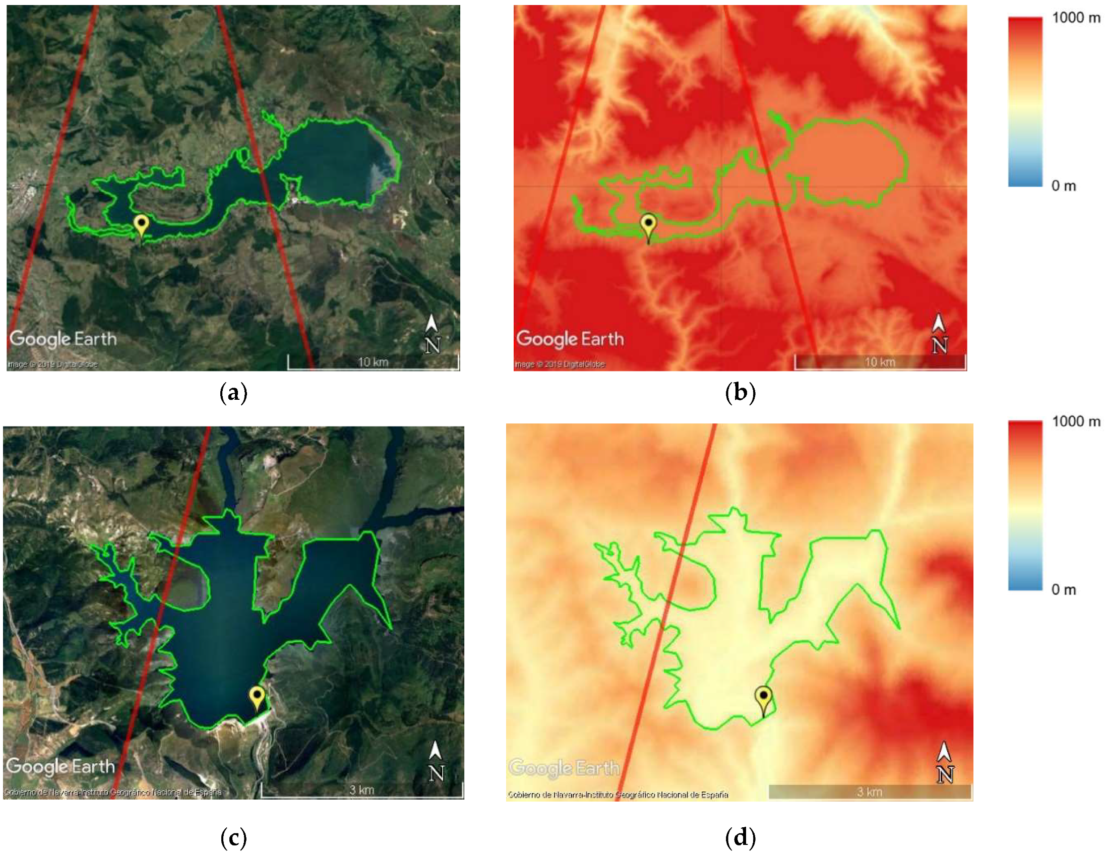
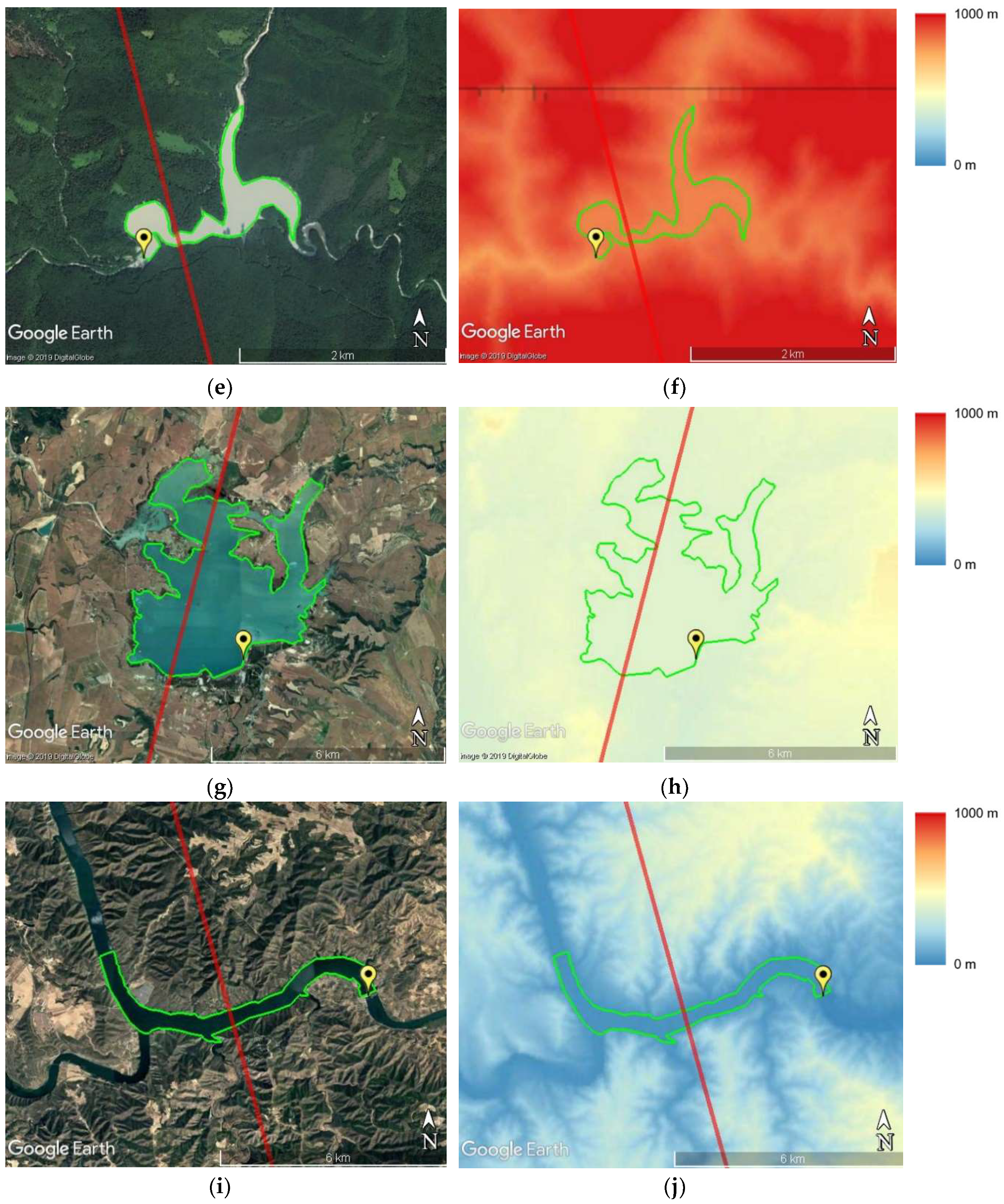
2.1. Study Area

Our study area encompassed the reservoirs and rivers in the Ebro River basin (Figure 1). The Ebro River, which has a length of approximately 910 km and a drainage basin with an area of approximately 85,362 km2, is one of the most important rivers on the Iberian Peninsula [68]. The river flow is irregular throughout the year, with low levels at the end of summer and high levels during the spring due to melt runoff in the Pyrenees, leading to a danger of flooding. The annual variation of the river flow is more than 800 m3 s−1 at Ribarroja dam, which is the last dam controlling the water flow entering the Mediterranean Sea [69]. The Ebro River is of great importance for agriculture in summer, during which drought often occurs due to the continental Mediterranean climate. Nevertheless, the mean annual flow has decreased by approximately 29% during the 20th century due to many causes: the construction of dams, the increasing demands for irrigation, and evaporation, the latter being higher than the precipitation due to low rainfall amounts, high sunshine intensities and strong, dry winds, from reservoirs within the river basin [68].
The Pyrenees mountain range lies to the north of the Ebro River basin. Consequently, it is challenging to retrieve the water surface heights of the studied area as the water bodies are relatively small and are greatly influenced by the mountainous terrain. The selected water bodies, for which we have gauging stations for validation, are shown in Figure 1. The coordinates, the widths of the water bodies covered with satellite tracks, the approximate distances between the gauging station and satellite tracks, and the average slope within 5 km along the satellite track are listed in Table 2. The water bodies that can be retracked properly, along with their DEMs, are shown in Figure 2 along with the water masks, Sentinel-3 tracks and the location of gauging stations. Only tracks overpassing the upper stream of the river (before the dam) were considered, ensuring the results could be validated against the in situ measurements.

2.2. Data Base

2.2.1. Sentinel-3

Sentinel-3 is an ocean and land mission based on a constellation of two satellites (Sentinel-3A and Sentinel-3B). Sentinel-3A was launched on 16 February 2016, with data available beginning in June 2016. It was followed by Sentinel-3B, which was launched on 25 April 2018, with data available beginning in December 2018. In this study, two years of Sentinel-3A data were used from June 2016 to June 2018. The SRAL instrument is the main topographic sensor used to provide water level measurements, and, hence, it was used in our research. The detailed parameters of the Sentinel-3 SRAL can be found in [70]. To acquire altimeter measurements, the Sentinel-3 SRAL transmits pulses at a Ku-band frequency, which is complemented by a C-band frequency to correct range delay errors due to the varying density of electrons in the ionosphere [70]. Sentinel-3 has two operational modes: SAR mode and LRM. As the SAR mode is available globally, we could retrieve inland water levels over any area tracked by Sentinel-3. The SRAL tracks the surface in two different tracking modes, namely, closed loop and open loop tracking. For closed loop tracking, the altimeter range window is autonomously positioned based on an on-board near real-time (NRT) analysis of the previous SRAL waveform; in contrast, for open loop tracking, the altimeter range window is positioned using a priori knowledge of the surface height stored in the instrument in a one-dimensional along-track DEM. The tracking modes for the studied water bodies over the Ebro River basin are listed in Table 2.
Three levels of processed altimeter data are available: Level-0, Level-1 and Level-2 products. In our study, Level-1 non-time critical (NTC) 20 Hz data were used for the water level retrieval by the three retrackers (i.e., the threshold, OCOG and two-step physical-based retrackers), and Sentinel-3 Level-2 ocean retracked data from ESA were used for comparison.
The main objectives of the Level-2 processing of SAR mode data are to provide elementary retracked altimeter estimates of the oceans, coastal zones, ice sheets and sea ice elevations [71]. Different retracking algorithms are more suited to specific surfaces, that is, for ocean retracking, OCOG retracking, ice sheet retracking, ice retracking and sea ice retracking. Unfortunately, ice-related retracker results are not available for inland water bodies; hence, we used Sentinel-3 Level-2 ocean retracker results for comparison. Ocean retrackers try to fit theoretically modeled multi-look Level-1B (L1B) waveforms to real L1B SAR waveforms, thereby providing estimates of the epoch, composite sigma, amplitude and the mispointing angle [71].

2.2.2. In Situ Data

In situ data for the Ebro River basin are available in the Automatic Hydrological Information System, in Spanish known as the “Sistema Automático de Información Hidrológica”, or the SAIH Ebro data hub [72]. SAIH Ebro is an online system providing hourly and daily hydrological information, including river gauge data, reservoir levels, rainfall amounts and temperatures, over the Ebro River basin. Together with the Sentinel-3 passes, we studied eight water bodies in our research, as listed in Table 2. The in situ data were collected from June 2016 to June 2018 on an hourly basis.

2.2.3. Digital Elevation Model

A DEM was used as an ancillary dataset for the selection of the waveform portion. The Shuttle Radar Topography Mission (SRTM) is an international research effort that obtains DEM data on a near-global scale from 56°S to 60°N [73]. The SRTM provides global data at two resolutions: 1 arc-second (~30 m) and 3 arc-seconds (~90 m). In our study, 1 arc-second global elevation data, which offer a worldwide coverage of void-filled data at a resolution of approximately 30 m, were used. The DEMs of water bodies are shown in Figure 2. The vertical accuracy of SRTM DEM is about ±16 m (absolute) and ±6 m (relative) [73,74,75,76,77]. However, vertical accuracy of the data decreases with the increase in slope and elevation due to presence of large outliers and voids [75].

3. Methodology

3.1. Geophysical Corrections

The space-borne radar altimeter is an essential tool for monitoring the oceans, but it can also be used for inland water surfaces, including lakes and rivers. The principle of altimetry can be found in [78] with application of geophysical corrections. In this study, corrections for the wet troposphere, dry troposphere, ionosphere, solid earth tide, geocentric pole tide and ocean loading tide were considered, as discussed by Fernandes et al. [79], and the geoid correction was applied. As the objective of the study was to directly exploit official Sentinel-3 L1B data and compare against Level-2 official products, the use of the geophysical corrections available in the Level-2 product were considered. The detailed corrections and their ranges are listed in Table 3 [80]. The Geoid model used is the Earth Gravitational Model 2008 (EGM2008) [81].
To improve the altimeter range accuracy, which is related to the water level measurement accuracy, the waveform needs to be retracked precisely to determine the accurate tracking point located on the leading edge [87]. We tested three different retrackers, which are listed in Section 3.2, to find the tracking points precisely from the land-contaminated waveforms.

3.2. Retrackers

3.2.1. Threshold Retracker

The threshold retracker is a simple retracker based on an estimation of the epoch (the leading edge position) as a percentage of the maximum peak [46,88]. In principle, it works well when the maximum peak originates from a nadir water body. The epoch is calculated as the first sample or range bin that is above a percentage of the waveform peak. To provide a higher precision on the estimated epoch, a linear interpolation between the range bins adjacent to the threshold crossing is used as suggested in [46]:
e p o c h = n t h 1 + ( A p e a k η t h y ( n t h 1 ) ) / ( y ( n t h ) y ( n t h 1 ) )
where n t h is the first range bin of the waveform whose power, y ( n t h ) is right above the threshold ( A p e a k η t h ), A p e a k is the amplitude of the peak of the waveform, and η t h is defined as a threshold percentage (50% in our case). The term ( A p e a k η t h y ( n t h 1 ) ) / ( y ( n t h ) y ( n t h 1 ) ) in Equation (1) corresponds to the linear proportionality coefficient.

3.2.2. Offset Center of Gravity (OCOG) Retracker

The OCOG retracker [46,48] was designed to calculate the center of gravity of the reflected waveform based on the power levels in the bins. It is an empirical retracker that implements a combination of the center of gravity (COG) and a conventional offset to estimate the related epoch (the leading edge position). Three main parameters are estimated for the OCOG retracker: the COG, the window size (W) and the amplitude (A).
Frappart’s definition [24] was considered in our analysis using squares of the power samples:
C O G = n = n 1 n 2 n y 2 ( n ) n = n 1 n 2 y 2 ( n ) W = ( n = n 1 n 2 y 2 ( n ) ) 2 n = n 1 n 2 y 4 ( n ) A = n = n 1 n 2 y 4 ( n ) n = n 1 n 2 y 2 ( n )
where y ( n ) is the nth power sample of the input waveform, and n1 and n2 are the initial and end range bins or positions, respectively, in the waveform used for the OCOG parameter estimation.
The estimated epoch can then be implemented using the conventional OCOG definition of the epoch:
e p o c h = C O G W / 2

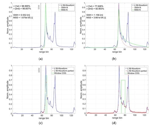
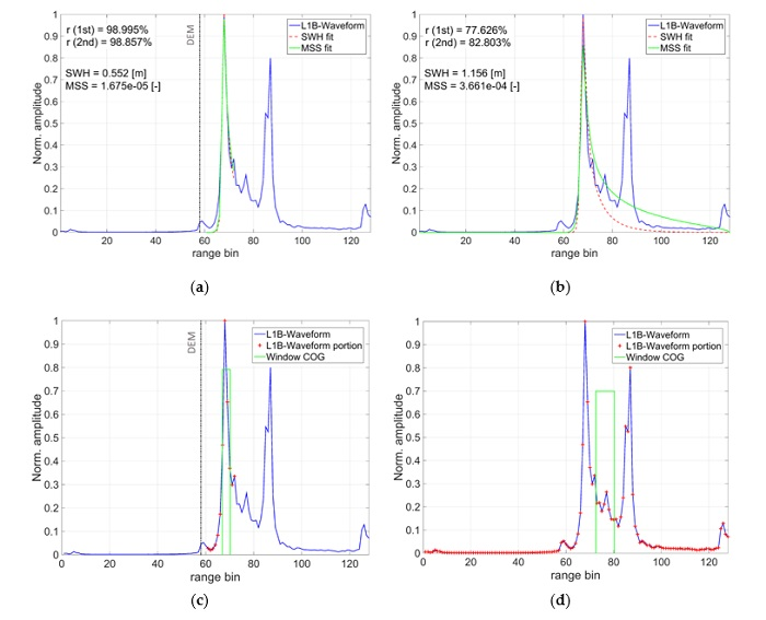
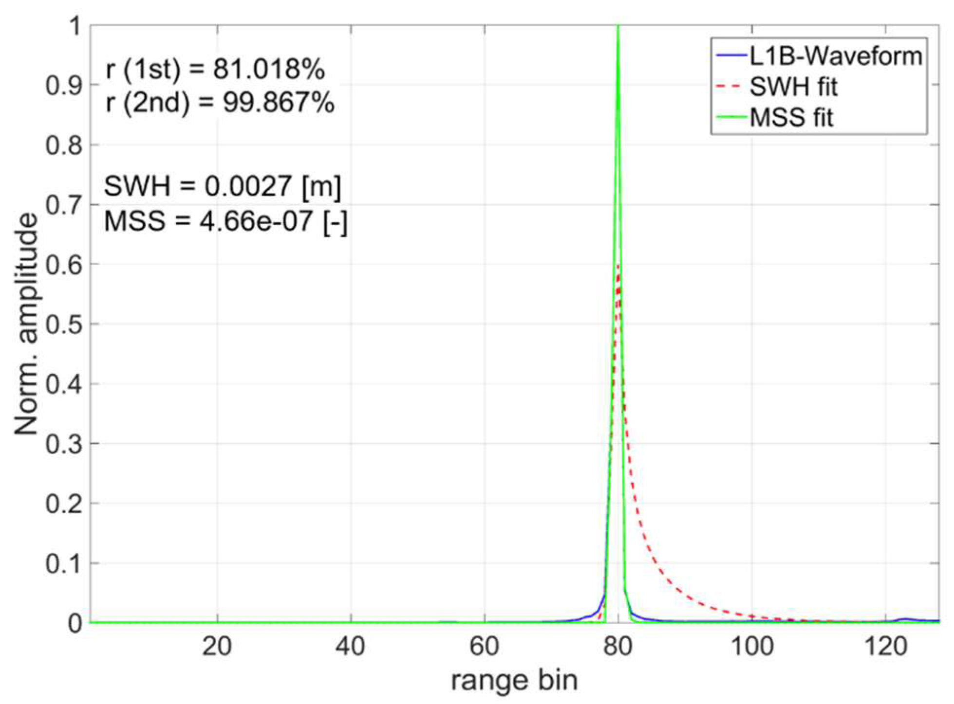
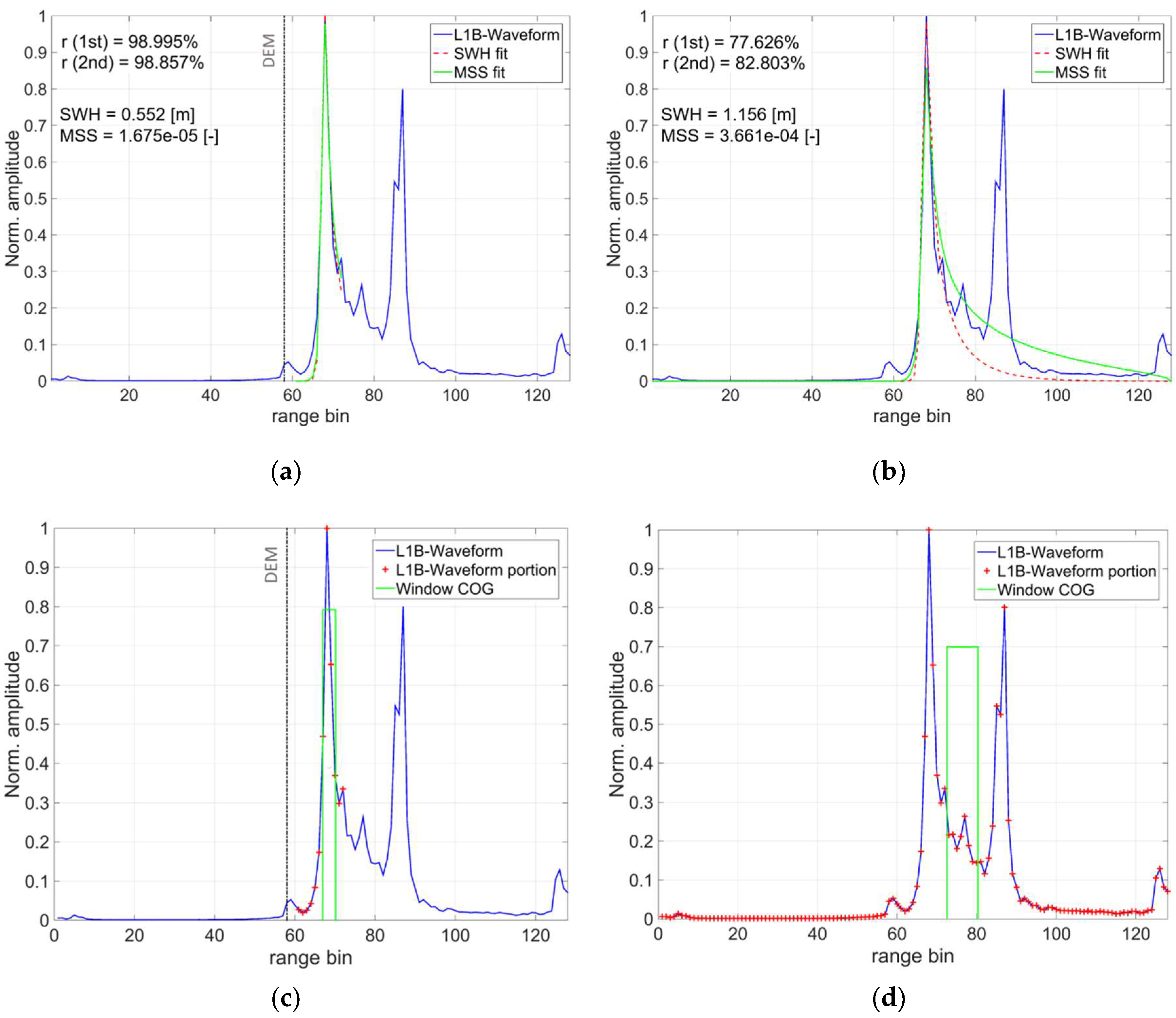
3.2.3. Two-Step Physical-Based Retracker

The in-house isardSAT SAR ocean retracker in [65] is integrated in a two-step fitting procedure to operate over inland waters, providing robust surface height estimation with a minimal modification to the SAR ocean retracker model. The waveforms reflected from an inland water body might exhibit ocean-like shapes (winds blowing over lakes) or, most commonly, a peakier shape (smoother surfaces) for small water bodies. To adapt to the latter ones, the MSS, describing the sea surface roughness [66], was used instead of the SWH as a fitting parameter; this approach is initially considered in [59], when exploiting the SAMOSA model over Tibetan plateau lakes.
The SAR ocean retracker in [65] considers a scattering model of rough surface with Gaussian statistics, and so the normalized backscattering coefficient (surface radiation pattern) as function of the incidence angle θ i n c can be modeled as [67]:
σ 0 ( θ i n c ) = σ 0 ( 0 ) exp ( ( tan θ i n c ) 2 M S S )
where the MSS represents the variance of the surface slopes. From the relationship in Equation (4), it can determined that, when the variance of the surface slopes (MSS) is large, a broad surface radiation pattern is obtained (rough surfaces), while, when MSS tends to small values, the pattern is more directed as expected for specular returns (smooth surfaces). Therefore, the MSS can be accordingly adjusted as a fitting parameter to properly fit specular returns. With the objective of exploiting the SAR ocean retracker [65] with minimal changes over inland waters, the same retracker model can be used, but the SWH is fixed (to a value close to zero), while the MSS or surface roughness is fitted. A similar approach with the SAMOSA model is exploited in [89] to fit waveform returns from leads.
To ensure that the different typology of waveforms (ocean- and specular-like) can be fitted, a two-step retracking is implemented. In a first run, the normal operation of the physical-based retracker in [65] was considered, i.e., the SWH was one of the fitting parameters (keeping MSS constant). Then, a second run of the fitting was implemented but this time the SWH was fixed (to a very small value around 1e-5) and the MSS was fitted so that the radiation pattern of the rough surface was adjusted. Then, the estimate of the surface height was extracted from the fit with the best correlation coefficient between the measured waveform and the modeled waveform. In this way, it was ensured that peaky-like waveforms could be properly fitted using the MSS as a fitting parameter, since the normal SAR ocean retracker would fail to adjust the model. An example of the operation of the two-step retracker is shown in Figure 3 over a peaky waveform.
The in-house isardSAT SAR ocean retracker integrated in the two-step procedure [65] is an implementation based on the SAR ocean model proposed by Chris Ray et al. [53]. It is a physically-based model of the altimetric power waveform over the ocean received by the altimetric sensor after delay-Doppler (or SAR) processing. Details regarding the definition and implementation of this retracker can be found in [65].
In SAR or delay-Doppler altimetry, different Doppler beams, also known as looks ( l ), are synthesized to focus on a given surface on the ground [65]. Thus, averaging of all these Doppler power beams would lead to the final multilook power waveform to be retracked. Therefore, for this physical-based retracker, each single-look power waveform was modeled as follows:
P ( k , l ) ( P u , k 0 , S W H / M S S )       = P u B ( k , l ) ( M S S ) ( g l ( S W H ) ) [ f 0 ( g l ( S W H ) ( k k 0 ) )       + T ( k , l ) ( M S S ) g l ( S W H ) σ z 2 L z 2 f 1 ( g l ( S W H ) ( k k 0 ) ) ]
where k refers to the range index vector within the received waveform window, l is the Doppler index or beam pointed to the specific surface, P u is the amplitude, k 0 is the epoch (related to the surface height), SWH is the significant wave height (referred also as H s ), and MSS is the mean square slope related to the surface roughness. In the first iteration of the two-step retracker, P u ,   k 0 , S W H are the fitting parameters, while in the second iteration the parameters being adjusted are P u , k 0 , M S S .
The terms B k , l and T k , l encompass the information related to the antenna pattern, antenna mis-pointing, and surface radiation patterns. They are obtained, respectively, as the constant and first order terms of a Taylor approximation of the antenna and surface radiation pattern’s product. The closed expression for these two terms can be found in [65]. A Gaussian-like antenna and surface radiation (as indicated in Equation (5)) patterns were assumed.
In Equation (5), g l   refers to the Doppler-dependent ( l ) dilation term, and takes into account the instrument configuration and the significant wave height:
g l = 1 σ a c 2 + ( 2 σ a l L x 2 L y 2 l ) 2 + σ z 2 / L z 2
where σ a c and σ a l refer to the widths of the Gaussian functions that approximate the point target response in the across-track (or range) and along-track (azimuth) dimensions, respectively, and σ z corresponds to the standard deviation of the sea surface height probability density function (PDF) and is related to the SWH as σ z = H s 4 . The definition of the additional terms in Equation (6) can be found in Table 4, where the main parameters of the SAR ocean model are summarized.
Finally, f 0 and f 1 represent the range-dependent functions modulated by the Doppler-dependent dilation term and can be obtained from the general expression (for n = 0 and 1):
f n ( ψ ) = 0 ( v 2 Ψ ) n e ( v 2 Ψ ) 2 2 d v  

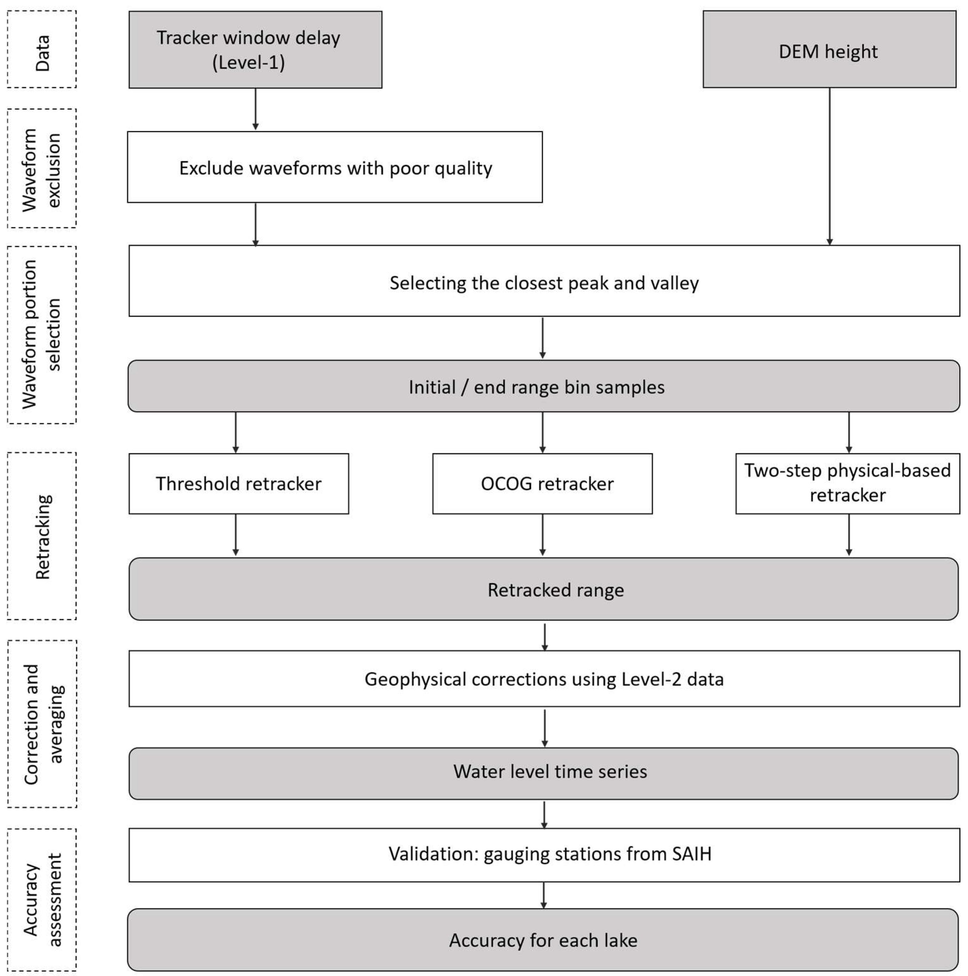
3.3. Waveform Exclusion

For very small water bodies, the waveform may be highly contaminated by the land. Thus, we added additional conditions to exclude the waveforms with a poor quality.
First, if the epoch of the reference SRTM DEM is outside the waveform window, which has a measuring range of approximately 60 m, it is likely that the on-board tracker window was unable to focus on the reflecting surface. Second, within the vicinity of land, reflections from both water and land will contribute to the received waveform, resulting in more than one peak. If the number of outstanding peaks is larger than a threshold, the waveform may be contaminated substantially by land or contains no water information at all, making it not suitable for water level retrieval. In our case, the threshold was set to 5 based on the analysis of waveforms. The number of outstanding peaks is normally less five, even with land contaminations. Finally, sigma_0, which is the backscatter coefficient for water from nadir, should be much larger than the backscatter coefficient for land, where the value is normally less than 50 dB based on the analysis in our study area. With these conditions (summarized below), we could filter out highly contaminated waveforms that were unsuitable for detecting the levels of water bodies:
  • The epoch of the reference SRTM DEM must be within the waveform window
  • Number of outstanding peaks < 5
  • Sigma_0 (backscatter coefficient) > 50 dB
After waveform exclusion, only the remaining waveforms (including both slightly contaminated and clean waveforms) were considered in our study to maximize the usage of the available measurements in the water body of interest. For a small water body, the quality of the waveform largely depends on the satellite tracks which drift daily, and the surface area changes with seasons, resulting in no clean waveform from time to time.

3.4. Selection of the Waveform Portion

Over inland water bodies, the on-board tracker may not properly locate the retrieval window to acquire the signal from the nadir corresponding to the water body. In addition, specific across-track surface contamination will be present in the waveforms, making it difficult to properly track the desired portion of the waveform. In our study, we used DEM information (SRTM DEM at a resolution of 30 m) to locate the waveform portion that comes from nadir within the receiving window, and then retracked the waveform using the selected portion only. This pre-processing approach, which prepares the portion of waveforms, can be applied and integrated with any kind of retracker.
The waveform portion selection method isolates the nadir return within the receiving window as follows:
  • From the geo-located surface of interest within the water body and beneath the satellite track, the associated height was interpolated from the DEM information and referred to the geodetic ellipsoid, H D E M .
  • This height was subtracted from the satellite height ( H o r b ) at the geo-located surface to obtain a rough estimation of the range (or equivalently window delay) from where the nadir returns were expected.
  • This range was linked to a specific bin within the received waveform, by comparing it with the vector of ranges associated to each bin in the receiving window, which could be obtained from the measured range by the radar and the range sampling.
  • The peak location closest to the previous range bin position was taken, and the portion of the waveform was selected around this peak considering the valley positions to the left and right of the peak plus some guard samples on top:
    A built-in Matlab function (findpeaks) was used to compute the prominent or outstanding peaks within the waveform. Prominent peaks are those peaks that drop more than a given threshold value on either side of the peak before the signal attains a higher value.
    The associated valley locations can be extracted using this built-in function, but taking as input the maximum of the whole waveform minus the waveform itself.
The water level for each footprint was retrieved based on the selected portion of the waveform applying the three retrackers. The time series of the water levels were calculated using a strict water mask polygon as shown in Figure 2, within which the water levels of the altimeter footprints were considered, selected and averaged for each track. The water mask polygon was created manually according to the shoreline displayed in the Google Earth image.
The workflow of the water level retrieval using the Sentinel-3 Level-1 product included four main steps: waveform exclusion, selecting the waveform portion using a DEM determining the retracking range using different retrackers, geophysical corrections and water level averaging, as shown in Figure 4. Geophysical corrections were applied to the retracked range using the Sentinel-3 Level-2 product, and the accuracy was assessed for each water body using in situ measurements from the gauging stations in the SAIH system.

4. Results

4.1. Selecting the Waveform Portion Using a DEM

When a waveform is influenced by land-based contamination, the waveform will contain small peaks due to off-nadir land or land coverage that follow the large peak, which corresponds to the water reflection within the altimeter footprint. In this case, as shown in Figure 5 (two outstanding peaks in Figure 5 waveform), the portion of the selected waveform provided a more precise tracking point for the two-step physical-based retracker and OCOG retracker, especially for the OCOG retracker, whose retracking point was the front edge of the COG window. The footprint of the signal was very close to the shore, thereby introducing a large peak at the trailing edge. The DEM information was used to select the portion of the waveform closer to nadir. The closest peak and valley after nadir were selected for retracking. Figure 5a,c shows the location of nadir in a black vertical line. The portion being selected is under the SWH fitting or MSS fitting line in Figure 5a with the two-step physical-based retracker, and is marked out in red crosses as the L1B-Waveform portion in Figure 5c with OCOG retracker. For the two-step physical-based retracker, the fitting using the selected waveform portion (Figure 5a) resulted in a 99% accuracy, while the fitting using the whole waveform (Figure 5b) resulted in an accuracy of 83%, making the location of the tracking point on the leading edge slightly different. In this study, the objective of the two-step physical-based retracker was to ensure proper retrieval of the surface height over inland waters, when exploiting the SAR ocean retracker in [65] with minimal changes on its operation; the significance and interpretation of other geophysical parameters that can be inferred (SWH and MSS) needs to be further investigated and it is out of the scope of the current study.
For the OCOG retracker, the COG when using the selected waveform portion was located inside the first peak. However, when using the whole waveform, it was located in between peaks, resulting in different tracking points that were the front edge of the COG window. For the threshold retracker, the tracking point did not change in this case. The threshold retracker depended only on the largest peak, which, as shown in Figure 5, was the same with or without waveform portion selection. However, in the case of the largest peak not being from the nadir water body but from the surroundings or other objectives, the threshold retracker with and without waveform portion selection led to different results.
The differences between the performance using the waveform portion selection method, and the method using the whole waveform, are shown in the time series results over the Ebro Reservoir in Figure 6. The Level-2 data were obtained from the Sentinel-3 Level-2 product using the ocean retracker, which does not include any waveform portion selection. The waveform portion selection method eliminated most outliers compared with the method of using the whole waveform.

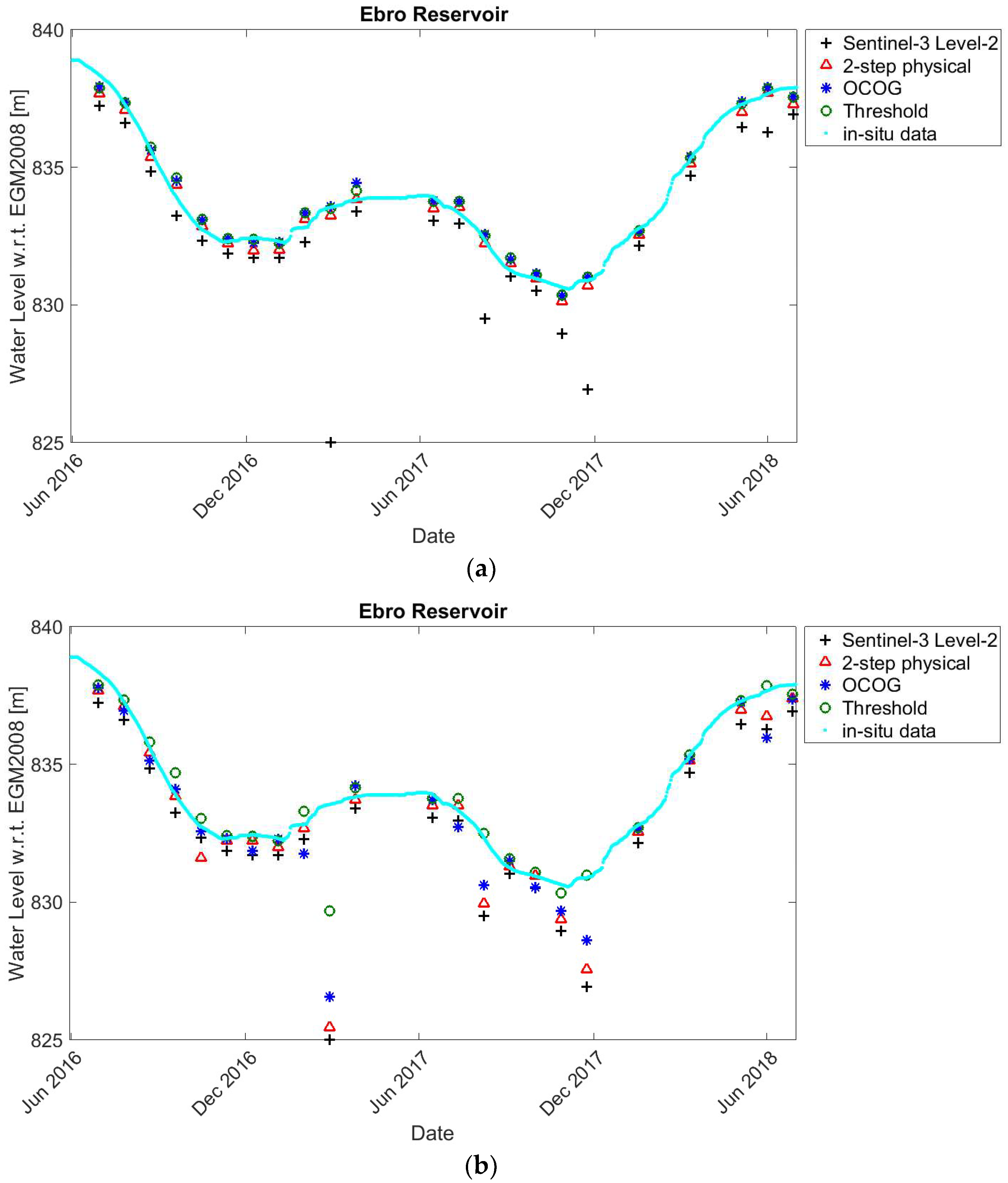
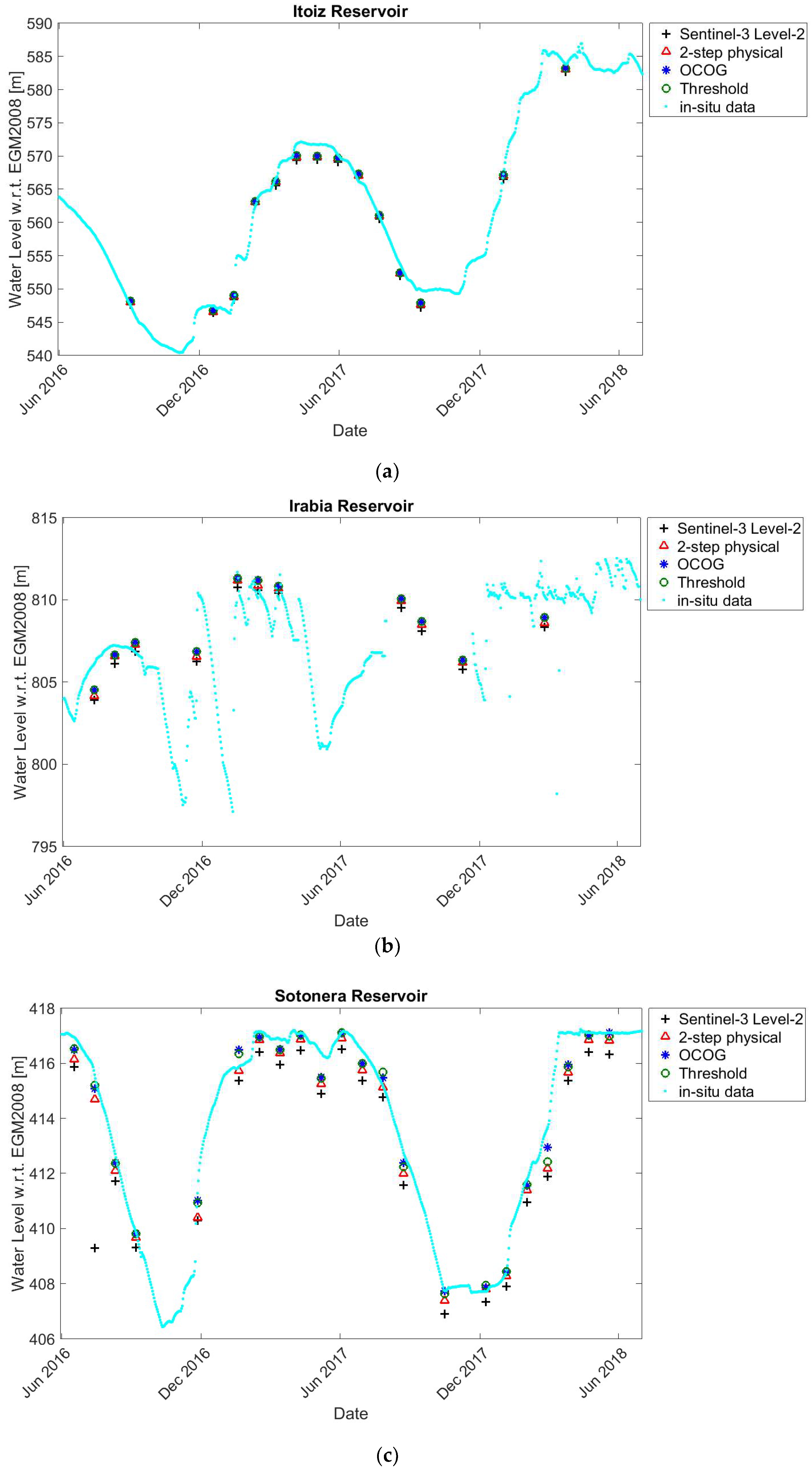
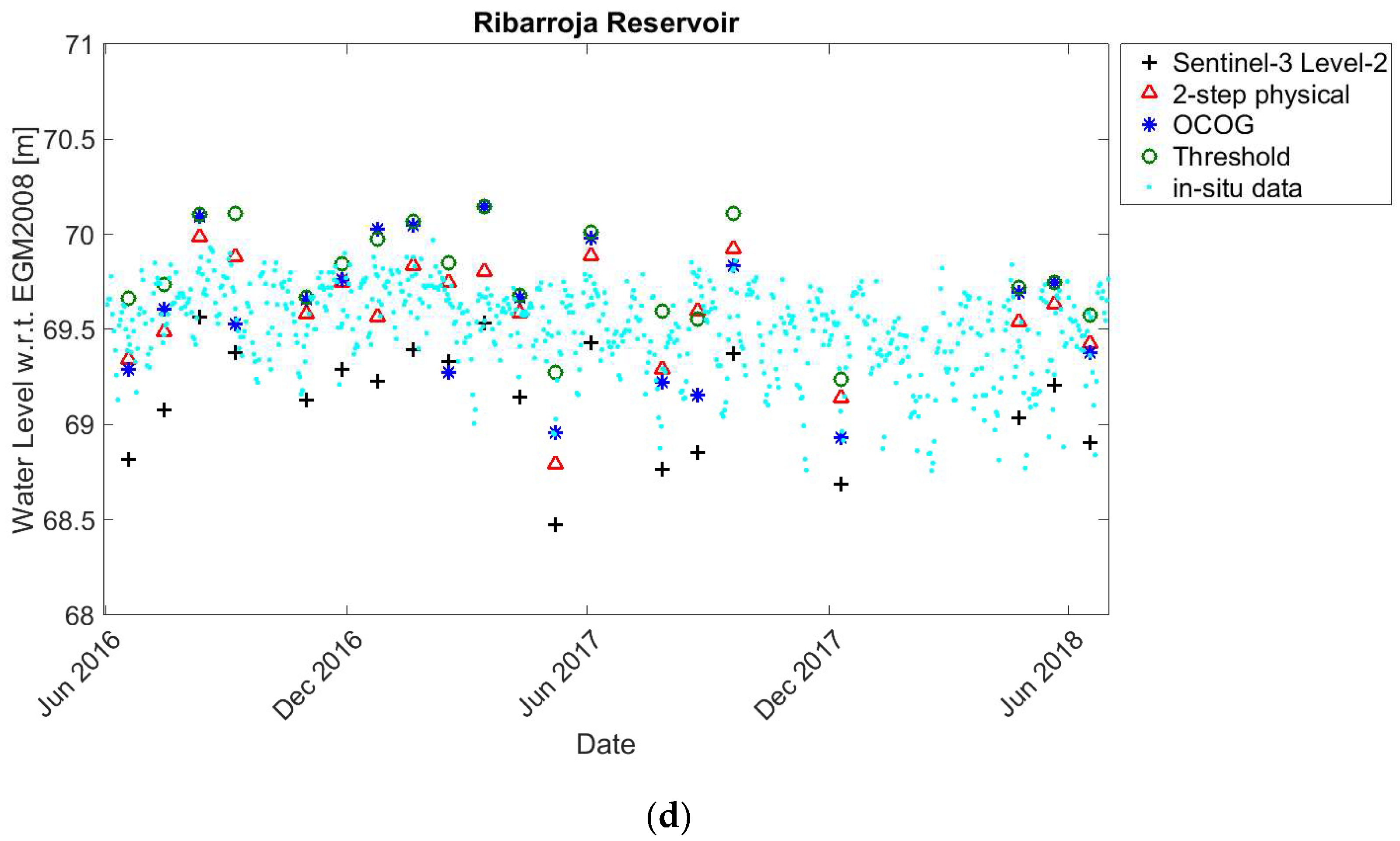
4.2. Time Series Validation

The time series of the water levels were calculated using a strict water mask polygon. The water levels of the altimeter footprints within the mask were considered, selected and averaged for each date. Figure 6a and Figure 7 show the water levels for different water bodies derived using the three retrackers: the two-step physical-based retracker, OCOG retracker and threshold retracker, combined with the waveform portion selection method. The retracked results were compared with the in situ measurements and the Level-2 results using the ocean retracker.
Among the eight water bodies monitored in this study, the water levels over the Mequinenza Reservoir, Cavallers Reservoir and San Salvador Reservoir, all of which were tracked in an open loop tracking mode (on-board DEM dependent), could not be retracked. The difference between the on-board tracking heights derived from the received waveforms and the heights from the SRTM DEM with reference to the geodetic ellipsoid was almost 50 m over the Mequinenza Reservoir, more than 1000 m over the Cavallers Reservoir, and approximately 80 m over the San Salvador Reservoir. These findings indicate that the SRAL sensor lost its track and was unable to acquire the waveforms reflected from these water body surfaces.
The RMSE and unbiased RMSE (ubRMSE) (Equation (8)) were calculated, as listed in Table 5. The unbiased RMSE is more reliable as it removes the bias.
u b R M S E = E { [ ( W L E [ W L ] ) ( i n s i t u E [ i n s i t u ] ) ] 2 }
where E[·] is the expectation operator and WL is the water level derived from satellite data. The RMSEs for different water bodies varied from 17 cm to more than 1 m. A comparison of the performances for the different retrackers over different water bodies is shown in Table 5. The best result was obtained for the Ribarroja Reservoir, which had an ubRMSE of approximately 16 cm. The results over the Ebro Reservoir, Sotonera and Ribarroja Reservoirs were also satisfactory. The RMSEs for the Itoiz Reservoir and Irabia Reservoir were relatively large with values greater than 1 m. The results using the three different retrackers do not show large differences except for the Sotonera Reservoir and Ribarroja Reservoir. The OCOG retracker gave the smallest ubRMSE for the Sotonera Reservoir with a value of approximately 38 cm. The two-step physical-based retracker and threshold retracker performed better over the Ribarroja Reservoir than the OCOG retracker, which had an ubRMSE of approximately 16 cm. All retrackers gave better results than the Level-2 ocean retracker without the waveform portion selection method.

5. Discussion

In this study, the size of the target water bodies vary from 130 m to 4.5 km and change with seasons. The geometries of the water bodies are complex with irregular lake shores and various sizes, making the along-track width (the width as seen by the satellite flying along the water body) very different from one satellite overpass to another due to the drifting satellite ground tracks. As a result, continuous clean waveforms rarely exist in our study area.
The shore of the Ebro Reservoir is irregular, and lands exist within water, resulting in no clean waveforms available over many tracks. Figure 6b shows the water level time series derived using the whole waveform, while Figure 6a shows the water level time series derived using the waveform portion selection. Retracking of the waveform portion accordingly reduced land contamination effects on the waveform. Figure 6a shows higher consistency with in situ time series, and thus shows that most of the outliers were caused by the land contamination. The land contaminated waveforms can be originated by surface area changes or satellite track drifting, making the altimeter footprint closer to the side bank, introducing outliers in the time series.
Over the water bodies where Sentinel-3 is operated in closed loop, the water levels of all water bodies could be tracked. Over the water bodies where Sentinel-3 is operated in open loop, three water bodies were missed and only one was tracked accurately. The results over the Ebro Reservoir, Sotonera and Ribarroja Reservoirs are satisfactory. The Ebro Reservoir is located in the north near the Pyrenees mountain range with elevations exceeding 820 m, and an average slope within 5 km along track of about 4%. The RMSE was 30 cm compared with the in situ measurements. The Sotonera Reservoir is the biggest reservoir studied, and is located in a relatively flat area with a slope of about 3% and an elevation of about 410 m. The result is good as there is no influence from the mountainous terrain, and it is big enough to be well monitored by satellite. The Ribarroja Reservoir is only 400 m wide and with a slope of more than 20%, but an elevation of only around 70 m. Its small width results in only one altimeter footprint per track available within the water body. The ubRMSE of Ribarroja Reservoir shows very good performance with a value of about 16 cm. However, the results for a few tracks were excluded due to poor waveform quality, which may be influenced by the rapid changes of surrounding terrain. The RMSEs over the Itoiz Reservoir and Irabia Reservoir exceeds 1 m. One reason for this could be the rapid change in the elevations along the satellite track as both water bodies are located in the Pyrenees, making it easy for a satellite to lose its track. The width of the Itoiz Reservoir with satellite data varies from 400 m to more than 2 km depending on the different satellite tracks, which drift daily. In addition, the Irabia Reservoir is a very small water body with a width of approximately 130 m, making the retrieval of its surface height more challenging. Besides the waveform quality, the size of the water body and the surrounding terrain, another reason for the differences with in-situ data from the gauging station is the distance between the gauging station and the Sentinel-3 tracks, varying from a few meters to several kilometers. Satellite tracks are always drifting (up to 1.5 km), making the footprints always changing in their locations for each water body. With the altimetry mission originally designed for ocean, the accuracy of geophysical corrections over inland water ranges from a few centimeters to tens of centimeters, depending on the size of the water body and wind conditions [79,90,91]. These effects will most definitely influence the final results, and need to be further considered quantitatively.
The results of the three retrackers, in combination with the waveform portion selection method, always give better accuracies than the results of the Sentinel-3 Level-2 ocean retracker (the results of both sets of retrackers are shown in Figure 6 and Table 5). Therefore, given the lack of an ice retracker over inland water bodies, retrieving the water levels by retracking the Level-1 waveforms and using the waveform portion selection method constitutes an alternative approach to obtain more accurate water levels.
The waveform portion selection method using DEM information greatly improved the results shown in both Figure 5 and Figure 6. As mentioned above, the vertical accuracy of SRTM DEM is approximately ±16 m (absolute) and ±6 m (relative). In the case of a 6 m error, the difference of choosing the right peak corresponding to nadir would be about 3 m. Therefore, if two large peaks were very close to each other, the portion of the waveform chosen might not be accurate. However, for most cases, the DEM error is small compared to the waveform tracking window, which is more than 60 m, and thus optimistic results can be obtained. Besides, waveform portion selection using DEM information improved the water level results over water bodies where only a few or no clean waveforms are available, and retained more results to have a better complete time series. In the case of the water level changing enormously and the waveform being heavily contaminated at the same time, the waveform portion selection approach may lose its capability of precise retracking.
The different retrackers obtained a good accuracy with in situ measurements. The ubRMSEs showed smaller values compared with RMSEs for all retrackers over different reservoirs, as listed in Table 5. The bias between the retrieved water levels and the in situ measurements existed in most cases, which may be related to the drift of the river course (the measurements are not co-located with the Sentinel-3 track). Other error sources include the waveform quality, which depends on the surrounding terrain. These include the geometry of the lake shore and the characteristics of the terrain, all of which contribute to the shape of the waveform. Nevertheless, Sentinel-3 has been proven to work for small water bodies.
We detected some issues related to the Sentinel-3 SRAL tracking mode. The open loop tracking mode, which depends on the on-board DEM to locate the tracking window, loses its track over the Cavallers Reservoir, which is surrounded by mountains, but also in Mequinenza and San Salvador Reservoirs, which are in relatively flat areas. We provided the correct water level height information to make Sentinel-3 able to capture the correct water level in the open loop tracking mode using the service altimeter open loop tracking command for hydrology monitoring (https://www.altimetry-hydro.eu/). We optimistically expect the water bodies that are under the Sentinel-3 coverage, but with loss of track, will be monitored in the near future. Another potential solution could be changing the tracking mode to a closed loop mode.

6. Conclusions

The objective of this study was to develop a methodology that can estimate water levels in small water bodies (similar size to the along-track resolution) and/or complex topography environments where many waveforms are expected to be contaminated by land. The study compared the performances of the threshold, OCOG and two-step physical-based retrackers, but no significant differences were found in the results of the three retrackers. However, the main improvements found show that selecting the portion of the waveform to be fitted significantly affected the retrievals.
The novel DEM-oriented waveform portion selection method could isolate the nadir peak from land-based contamination relatively well, and greatly improved the results with a reduction of RMSE by more than 0.5 m over Ebro Reservoir. Retracking the water levels from Level-1 waveforms using the combination of a retracker and the waveform portion selection method was more robust to land contamination than using Sentinel-3 Level-2 data directly. It also resulted in a better accuracy.
The water levels were compared with in situ measurements and the Sentinel-3 Level-2 ocean retracker from ESA. The results show good agreement with the in situ measurements. The ubRMSE over the Ribarroja Reservoir with a width of about 400 m could reach 16 cm, while that over the Ebro Reservoir whose width is about 1.8 km, it could reach 28 cm. Waveform portion selection using DEM information showed its ability to retrieve water levels over small- to medium-sized water bodies. In contrast, the accuracy over water bodies located in mountainous areas still needs to be improved, but the results demonstrate the possibility of retrieving the water levels over a very small water body with a width of approximately 130 m.
Overall, the Sentinel-3 SRAL has been proven to work over inland water bodies, even those with widths as small as 130 m. Retracking using the waveform portion selection method with an SRTM DEM as a pre-processing to the two-step physical-based retracker, the OCOG retracker and threshold retracker improved the accuracy with an optimal ubRMSE of 16 cm. Further steps need to be taken to explore the possibilities for both tracking water bodies that are not currently being tracked, and for improving the accuracies for very small water bodies with Sentinel-3 altimeter data.

Author Contributions

Q.G., E.M. and M.J.E. conceived, designed and implemented the research. Q.G. and E.M. coded the program. Q.G. performed the analysis of the data and drafted the manuscript. M.J.E. assisted in the data analysis and interpretation. All authors reviewed and improved the manuscript. The study was supervised by M.J.E.

Funding

Qi Gao received grant DI-15-08105 from the Spanish Education Ministry (MICINN) and DI-2016-078 from the Catalan Agency of Research (AGAUR). This work was partially funded by the Spanish Ministry of Science, Innovation and Universities and the European Regional Development Fund through grant CGL2017-85687-R.

Acknowledgments

The authors wish to thank the technical teams for their support, the Copernicus Programme, which provided open access to the Sentinel data, and the SAIH Ebro team, who provided the ground information.

Conflicts of Interest

The authors declare no conflict of interest.

References

  1. Postel, S.L.; Carpenter, S.R. Freshwater Ecosystem Services. In Nature’s Services; Daily, G., Ed.; Island Press: Washington, DC, USA, 1997; pp. 195–214. [Google Scholar]
  2. Döll, P.; Hoffmann-Dobrev, H.; Portmann, F.T.; Siebert, S.; Eicker, A.; Rodell, M.; Strassberg, G.; Scanlon, B.R. Impact of water withdrawals from groundwater and surface water on continental water storage variations. J. Geodyn. 2012, 59, 143–156. [Google Scholar] [CrossRef]
  3. Alsdorf, D.E.; Rodriguez, E.; Lettenmaier, D.P. Measuring surface water from space. Rev. Geophys. 2007, 45, RG2002. [Google Scholar] [CrossRef]
  4. Gleick, P.H. Global freshwater resources: Soft-path solutions for the 21st century. Science 2003, 302, 1524–1528. [Google Scholar] [CrossRef] [PubMed]
  5. Bogning, S.; Frappart, F.; Blarel, F.; Niño, F.; Mahé, G.; Bricquet, J.-P.; Seyler, F.; Onguéné, R.; Etamé, J.; Paiz, M.-C.; et al. Monitoring Water Levels and Discharges Using Radar Altimetry in an Ungauged River Basin: The Case of the Ogooué. Remote Sens. 2018, 10, 350. [Google Scholar] [CrossRef]
  6. Benveniste, J. Radar Altimetry: Past, Present and Future. In Coastal Altimetry; Vignudelli, S., Kostianoy, A., Cipollini, P., Benveniste, J., Eds.; Springer: Berlin/Heidelberg, Germany, 2011; ISBN 978-3-642-12795-3. [Google Scholar] [CrossRef]
  7. Calman, S.; Seyler, F. Continental surface water from satellite altimetry. C. R. Geosci. 2006, 338, 1113–1122. [Google Scholar] [CrossRef]
  8. Cretaux, J.F.; Birkett, C. Lake studies from satellite radar altimetry. C. R. Geosci. 2006, 338, 1098–1112. [Google Scholar] [CrossRef]
  9. Radar Altimetry Tutorial and Toolbox—A Collaborative Portal for Altimetry Users. Available online: http://www.altimetry.info/ (accessed on 3 November 2018).
  10. Raney, R.K. The delay/Doppler radar altimeter. IEEE Trans. Geosci. Remote Sens. 1998, 36, 1578–1588. [Google Scholar] [CrossRef]
  11. Wingham, D.J.; Phalippou, L.; Mavrocordatos, C.; Wallis, D. The mean echo and echo cross-product from a beam forming, interferometric altimeter and their application to elevation measurement. IEEE Trans. Geosci. Remote Sens. 2004, 10, 10–2323. [Google Scholar] [CrossRef]
  12. Koblinsky, C.J.; Clarke, R.T.; Brenner, A.C.; Frey, H. Measurement of river level variations with satellite altimetry. Water Resour. Res. 1993, 29, 1839–1848. [Google Scholar] [CrossRef]
  13. Birkett, C. The contribution of TOPEX/POSEIDON to the global monitoring of climatically sensitive lakes. J. Geophys. Res. Ocean. 1995, 100, 25179–25204. [Google Scholar] [CrossRef]
  14. Birkett, C.M. Contribution of the TOPEX NASA radar altimeter to the global monitoring of large rivers and wetlands. Water Resour. Res. 1998, 34, 1223–1239. [Google Scholar] [CrossRef]
  15. Jarihani, A.A.; Callow, J.N.; Johansen, K.; Gouweleeuw, B. Evaluation of multiple satellite altimetry data for studying inland water bodies and river floods. J. Hydrol. 2013, 505, 78–90. [Google Scholar] [CrossRef]
  16. Yi, Y.; Kouraev, A.V.; Shum, C.K.; Vuglinsky, V.S.; Cretaux, J.F.; Calmant, S. The performance of altimeter waveform retrackers at Lake Baikal. Terr. Atmos. Ocean. Sci. 2013, 24, 513–519. [Google Scholar] [CrossRef]
  17. Nielsen, K.; Stenseng, L.; Andersen, O.B.; Villadsen, H.; Knudsen, P. Validation of CryoSat-2 SAR mode based lake levels. Remote Sens. Environ. 2015, 171, 162–170. [Google Scholar] [CrossRef]
  18. Schwatke, C.; Dettmering, D.; Boergens, E.; Bosch, W. Potential of SARAL/AltiKa for inland water applications. Mar. Geod. 2015, 38, 626–643. [Google Scholar] [CrossRef]
  19. Villadsen, H.; Andersen, O.; Stenseng, L.; Nielsen, K.; Knudsen, P. CryoSat-2 altimetry for river level monitoring—Evaluation in the Ganges-Brahmaputra River basin. Remote Sens. Environ. 2015, 168, 80–89. [Google Scholar] [CrossRef]
  20. Moore, P.; Birkinshaw, S.J.; Ambrózio, A.; Restano, M.; Benveniste, J. CryoSat-2 Full Bit Rate Level 1A processing and validation for inland water applications. Adv. Space Res. 2018, 62, 1497–1515. [Google Scholar] [CrossRef]
  21. Song, C.; Huang, B.; Ke, L. Inter-annual changes of alpine inland lake water storage on the Tibetan Plateau: Detection and analysis by integrating satellite altimetry and optical imagery. Hydrol. Process. 2014, 28, 2411–2418. [Google Scholar] [CrossRef]
  22. Song, C.; Ye, Q.; Sheng, Y.; Gong, T. Combined ICESat and CryoSat-2 altimetry for accessing water level dynamics of Tibetan lakes over 2003–2014. Water 2015, 7, 4685–4700. [Google Scholar] [CrossRef]
  23. Song, C.; Ye, Q.; Cheng, X. Shifts in water-level variation of Namco in the central Tibetan Plateau from ICESat and CryoSat-2 altimetry and station observations. Sci. Bull. 2015, 60, 1287–1297. [Google Scholar] [CrossRef]
  24. Frappart, F.; Calmant, S.; Cauhop, M.; Seyler, F.; Cazenave, A. Preliminary results of ENVISAT RA-2-derived water levels validation over the Amazon Basin. Remote Sens. Environ. 2006, 100, 252–264. [Google Scholar] [CrossRef]
  25. Villadsen, H.; Deng, X.; Andersen, O.B.; Stenseng, L.; Nielsen, K.; Knudsen, P. Improved inland water levels from SAR altimetry using novel empirical and physical retrackers. J. Hydrol. 2016, 537, 234–247. [Google Scholar] [CrossRef]
  26. Jiang, L.; Nielsen, K.; Andersen, O.B.; Bauer-Gottwein, P. Monitoring recent lake level variations on the Tibetan Plateau using CryoSat-2 SARin mode data. J. Hydrol. 2017, 544, 109–124. [Google Scholar] [CrossRef]
  27. Kleinherenbrink, M.; Ditmar, P.G.; Lindenbergh, R.C. Retracking CryoSat data in the SARIn mode and robust lake level extraction. Remote Sens. Environ. 2014, 152, 38–50. [Google Scholar] [CrossRef]
  28. Schwatke, C.; Dettmering, D.; Bosch, W.; Seitz, F. DAHITI—An innovative approach for estimating water level time series over inland waters using multi-mission satellite altimetry. Hydrol. Earth Syst. Sci. 2015, 19, 4345–4364. [Google Scholar] [CrossRef]
  29. Crétaux, J.-F.; Jelinski, W.; Calmant, S.; Kouraev, A.; Vuglinski, V.; Bergé-Nguyen, M.; Gennero, M.-C.; Nino, F.; Abarca Del Rio, R.; Cazenave, A.; et al. SOLS: A Lake database to monitor in Near Real Time water level and storage variations from remote sensing data. J. Adv. Space Res. 2011, 47, 1497–1507. [Google Scholar] [CrossRef]
  30. Birkett, C.M.; Reynolds, C.; Beckley, B.; Doorn, B. From Research to Operations: The USDA Global Reservoir and Lake Monitor; Vignudelli, S., Kostianoy, A.G., Cipollini, P., Benveniste, J., Eds.; Chapter 2 in Coastal Altimetry, Springer Publications; Springer: Berlin/Heidelberg, Germany, 2010; ISBN 978-3-642-12795-3. [Google Scholar]
  31. Gustafsson, D.; Andersson, J.; Brito, F.; Martinez, B.; Arheimer, B. New tool to share data and models in hydrological forecasting, based on the ESA TEP. In Proceedings of the EGU 2018 Symposium, Vienna, Austria, 8–13 April 2018. [Google Scholar]
  32. Dinardo, S.; Restano, M.; Ambrózio, A.; Benveniste, J. SAR Altimetry Processing on Demand Service for Cryosat-2 and Sentinel-3 at Esa G-Pod. In Proceedings of the 2016 conference on Big Data from Space (BiDS’16), Santa Cruz de Tenerife, Spain, 15–17 March 2016. [Google Scholar] [CrossRef]
  33. Birkinshaw, S.J.; O’Donnell, G.M.; Moore, P.; Kilsby, C.G.; Fowler, H.J.; Berry, P.A.M. Using satellite altimetry data to augment flow estimation techniques on the Mekong River. Hydrol. Process. 2010, 24, 3811–3825. [Google Scholar] [CrossRef]
  34. Da Silva, J.S.; Calmant, S.; Seyler, F.; Rotunno Filho, O.C.; Cochonneau, G.; Mansur, W.J. Water levels in the Amazon basin derived from the ERS 2 and ENVISAT radar altimetry missions. Remote Sens. Environ. 2010, 114, 2160–2181. [Google Scholar] [CrossRef]
  35. Michailovsky, C.I.; McEnnis, S.; Berry, P.A.M.; Smith, R.; Bauer-Gottwein, P. River monitoring from satellite radar altimetry in the Zambezi River Basin. Hydrol. Earth Syst. Sci. 2012, 9, 3203–3235. [Google Scholar] [CrossRef]
  36. Maillard, P.; Bercher, N.; Calmant, S. New processing approaches on the retrieval of water levels in Envisat and SARAL radar altimetry over rivers: A case study of the Sao Francisco River, Brazil. Remote Sens. Environ. 2015, 156, 226–241. [Google Scholar] [CrossRef]
  37. Boergens, E.; Nielsen, K.; Andersen, O.B.; Dettmering, D.; Seitz, F. River Levels Derived with CryoSat-2 SAR Data Classification—A Case Study in the Mekong River Basin. Remote Sens. 2017, 9, 1238. [Google Scholar] [CrossRef]
  38. Schneider, R.; Tarpanelli, A.; Nielsen, K.; Madsen, H.; Bauer-Gottwein, P. Evaluation of multi-mode CryoSat-2 altimetry data over the Po River against in situ data and a hydrodynamic model. Adv. Water Resour. 2018, 112, 17–26. [Google Scholar] [CrossRef]
  39. Huang, Q.; Long, D.; Du, M.; Zeng, C.; Li, X.; Hou, A.; Hong, Y. An improved approach to monitoring Brahmaputra River water levels using retracked altimetry data. Remote Sens. Environ. 2018, 211, 112–128. [Google Scholar] [CrossRef]
  40. Biancamaria, S.; Frappart, F.; Leleu, A.-S.; Marieu, V.; Blumstein, D.; Desjonquères, J.D.; Boy, F.; Sottolichio, A.; Valle-Levinson, A. Satellite altimetry water elevations performance over a 200 m wide river: Evaluation over the Garonne River. Adv. Space Res. 2017, 59, 128–146. [Google Scholar] [CrossRef]
  41. Becker, M.; da Silva, J.; Calmant, S.; Robinet, V.; Linguet, L.; Seyler, F. Water level fluctuations in the Congo Basin derived from ENVISAT satellite altimetry. Remote Sens. 2014, 6, 9340–9358. [Google Scholar] [CrossRef]
  42. Birkett, C.M.; Mertes, L.A.K.; Dunne, T.; Costa, M.H.; Jasinski, M.J. Surface water dynamics in the Amazon Basin: Application of satellite radar altimetry. J. Geophys. Res. 2002, 107, 8059. [Google Scholar] [CrossRef]
  43. Birkinshaw, S.J.; Moore, P.; Kilsby, C.G.; O’Donnell, G.M.; Hardy, A.J.; Berry, P.A.M. Daily discharge estimation at ungauged river sites using remote sensing. Hydrol. Process. 2014, 28, 1043–1054. [Google Scholar] [CrossRef]
  44. Cretaux, J.-F.; Calmant, S. Spatial Altimetry and Continental Waters. In Land Surface Remote Sensing in Continental Hydrology; Baghdadi, N., Zribi, M., Eds.; Elsevier: Amsterdam, The Netherlands, 2016. [Google Scholar] [CrossRef]
  45. Gommenginger, C.; Martin-Puig, C.; Amarouche, L.; Raney, R.K. Review of State of Knowledge for SAR Altimetry over Ocean; Report of the EUMETSAT JASON-CS SAR Mode Error Budget Study; National Oceanography Centre: Southampton, UK, 2013; Available online: https://eprints.soton.ac.uk/366765/ (accessed on 1 September 2018).
  46. Davis, C.H. A robust threshold retracking algorithm for measuring ice-sheet surface elevation change from satellite radar altimeter. IEEE Trans. Geosci. Remote Sens. 1997, 35, 974–979. [Google Scholar] [CrossRef]
  47. Martin, T.V.; Zwally, H.J.; Brenner, A.C.; Bindschadler, R.A. Analysis and retracking of continental ice sheet radar altimeter waveforms. J. Geophys. Res. Ocean. 1983, 88, 1608–1616. [Google Scholar] [CrossRef]
  48. Wingham, D.J.; Rapley, C.G.; Griffiths, H. New techniques in satellite tracking system. In Proceedings of the IGARSS’ 86 Symposium, Zurich, Switzerland, 8–11 September 1986; pp. 1339–1344. [Google Scholar]
  49. Bamber, J.L. Ice sheet altimeter processing scheme. Int. J. Remote Sens. 1994, 15, 925–938. [Google Scholar] [CrossRef]
  50. Brown, G.S. The average impulse response of a rough surface and its applications. IEEE Trans. Antennas Propag. 1977, 25, 67–74. [Google Scholar] [CrossRef]
  51. Legrésy, B.; Rémy, F. Altimetric observations of surface characteristics of the Antarctic ice sheet. J. Glaciol. 1997, 43, 265–275. [Google Scholar] [CrossRef]
  52. Legrésy, B.; Papa, F.; Remy, F.; Vinay, G.; Bosch, M.V.D.; Zanife, O.Z. ENVISAT radar altimeter measurements over continental surfaces and ice caps using the Ice-2 retracking algorithm. Remote Sens. Environ. 2005, 95, 150–163. [Google Scholar] [CrossRef]
  53. Ray, C.; Martin-Puig, C.; Clarizia, M.P.; Ruffini, G.; Dinardo, S.; Gommenginger, C.; Benveniste, J. SAR altimeter backscattered waveform model. IEEE Trans. Geosci. Remote Sens. 2015, 53, 911–919. [Google Scholar] [CrossRef]
  54. Fenoglio-Marc, L.; Dinardo, S.; Scharroo, R.; Roland, A.; Dutour Sikiric, M.; Lucas, B.; Becker, M.; Benveniste, J.; Weiss, R. The German Bight: A validation of CryoSat-2 altimeter data in SAR mode. Adv. Space Res. 2015, 55, 2641–2656. [Google Scholar] [CrossRef]
  55. Wingham, D.J.; Francis, C.R.; Baker, S.; Bouzinac, C.; Brockley, D.; Cullen, R.; de Chateau-Thierry, P.; Laxon, S.W.; Mallow, U.; Mavrocordatos, C.; et al. CryoSat: A mission to determine the fluctuations in Earth’s land and marine ice fields. Adv. Space Res. 2006, 37, 841–871. [Google Scholar] [CrossRef]
  56. Mavrocordatos, C.; Berruti, B.; Aguirre, M.; Drinkwater, M. The Sentinel-3 mission and its topography element. In Proceedings of the IEEE International Geoscience and Remote Sensing Symposium (IGARSS 2007), Barcelona, Spain, 23–27 July 2007; pp. 3529–3532. [Google Scholar] [CrossRef]
  57. Chander, S.; Ganguly, D.; Dubey, A.K.; Gupta, P.K.; Singh, R.P.; Chauhan, P. Inland Water Bodies Monitoring Using Satellite Altimetry Over Indian Region. ISPRS-Int. Arch. Photogramm. Remote Sens. Spat. Inf. Sci. 2014, 1035–1041. [Google Scholar] [CrossRef]
  58. Martin-Puig, C.; García, P. A new SAR altimetry waveform model in combination with phase information for coastal altimetry. In Proceedings of the 8th Coastal Altimetry Workshop, Lake Constance, Germany, 23–24 October 2014. [Google Scholar]
  59. Martin-Puig, C.; García, P. Synthetic Aperture Radar (SAR) altimetry for hydrology. In Proceedings of the ESA Living Planets Symposium, Edinburgh, Scotland, UK, 9–13 September 2013. [Google Scholar]
  60. Roca, M.; Martínez, D.; Reche, M. Preliminary results obtained using the EnviSat RA-2 individual echoes (full-rate waveforms with phase information). In Proceedings of the IEEE International Geoscience and Remote Sensing Symposium, Seoul, Korea, 25–29 July 2005. [Google Scholar] [CrossRef]
  61. Roca, M.; Martinez, D.; Reche, M. The RA-2 individual echoes processing description and some scientific results. In Proceedings of the IEEE International Geoscience and Remote Sensing Symposium, Barcelona, Spain, 23–27 July 2007; pp. 3541–3546. [Google Scholar] [CrossRef]
  62. Bramer, S.M.S.; Berry, P.A.M.; Freeman, J.A.; Rommen, B. Global Analysis of Envisat Ku and S Band Sigma0 over All Surfaces. In Proceedings of the Envisat Symposium, Montreux, Switzerland, 23–27 April 2007. [Google Scholar]
  63. Abileah, R.; Scozzari, A.; Vignudelli, S. Envisat RA-2 Individual Echoes: A Unique Dataset for a Better Understanding of Inland Water Altimetry Potentialities. Remote Sens. 2017, 9, 605. [Google Scholar] [CrossRef]
  64. Egido, A.; Smith, W.H.F. Fully Focused SAR Altimetry: Theory and Applications. IEEE Trans. Geosci. Remote Sens. 2017, 55, 392–406. [Google Scholar] [CrossRef]
  65. Makhoul, E.; Roca, M.; Ray, C.; Escolà, R.; Garcia-Mondéjar, A. Evaluation of the precision of different Delay-Doppler Processor (DDP) algorithms using CryoSat-2 data over open ocean. Adv. Space Res. 2018, 62, 1464–1478. [Google Scholar] [CrossRef]
  66. Li, S.; Zhao, D.; Zhou, L.; Liu, B. Dependence of mean square slope on wave state and its application in altimeter wind speed retrieval. Int. J. Remote Sens. 2013, 34, 264–275. [Google Scholar] [CrossRef]
  67. Valenzuela, G.R. Theories for the interaction of electromagnetic and oceanic waves—A review. Bound.-Layer Meteorol. 1978, 13, 61–85. [Google Scholar] [CrossRef]
  68. Romaní, A.M.; Sabater, S.; Muñoz, I. The Physical Framework and Historic Human Influences in the Ebro River. In The Ebro River Basin; The Handbook of Environmental Chemistry; Barceló, D., Petrovic, M., Eds.; Springer: Berlin/Heidelberg, Germany, 2010; Volume 13. [Google Scholar] [CrossRef]
  69. Cruzado, A.; Velasquez, Z.; Perez, M.; Bahamon, N.; Grimaldo, N.S.; Ridolfi, F. Nutrient fluxes from the Ebro River and subsequent across-shelf dispersion. Cont. Shelf Res. 2002, 22, 349–360. [Google Scholar] [CrossRef]
  70. Sentinel-3 Team. SentinSentinel-3 User Handbook. European Space Agency. Available online: https://earth.esa.int/documents/247904/685236/Sentinel-3_User_Handbook-iss1_v1_20170113/960ff616-87f5-43cc-b23e-3e96030bd13a (accessed on 15 March 2018).
  71. Re-Tracking Estimates. Available online: https://sentinel.esa.int/web/sentinel/technical-guides/sentinel-3-altimetry/level-2/re-tracking-estimates (accessed on 3 October 2018).
  72. SAIH Ebro. Available online: http://www.saihebro.com (accessed on 1 July 2018).
  73. Farr, T.G.; Rosen, P.A.; Caro, E.; Crippen, R.; Duren, R.; Hensley, S.; Kobrick, M.; Paller, M.; Rodriguez, E.; Roth, L.; et al. The Shuttle Radar Topography Mission. Rev. Geophys. 2007, 45. [Google Scholar] [CrossRef]
  74. Mukul, M.; Srivastava, V.; Mukul, M. Analysis of the accuracy of shuttle radar topography mission (SRTM) height models using international global navigation satellite system service (IGS) network. J. Earth Syst. Sci. 2015, 124, 1343–1357. [Google Scholar] [CrossRef]
  75. Mukul, M.; Srivastava, V.; Mukul, M. Uncertainties in the Shuttle Radar Topography Mission (SRTM) heights: Insights from the Indian Himalaya and Peninsula. Sci. Rep. 2017, 7, 41672. [Google Scholar] [CrossRef]
  76. Rabus, B.; Eineder, M.; Roth, A.; Bamler, R. The shuttle radar topography mission—A new class of digital elevation models acquired by space borne radar. J. Photogramm. Remote Sens. 2003, 57, 241–262. [Google Scholar] [CrossRef]
  77. Elkhrachy, I. Vertical accuracy assessment for SRTM and ASTER Digital Elevation Models: A case study of Najran city, Saudi Arabia. Ain Shams Eng. J. 2017. [Google Scholar] [CrossRef]
  78. Calmant, S.; Seyler, F.; Cretaux, J.F. Monitoring continental surface waters by satellite altimetry. Surv. Geophys. 2008, 29, 247–269. [Google Scholar] [CrossRef]
  79. Fernandes, M.J.; Lázaro, C.; Nunes, A.L.; Scharroo, R. Atmospheric Corrections for Altimetry Studies over Inland Water. Remote Sens. 2014, 6, 4952–4997. [Google Scholar] [CrossRef]
  80. Sentinel-3A L2P SLA Product Handbook. Available online: https://www.aviso.altimetry.fr/fileadmin/documents/data/tools/hdbk_L2P_S3.pdf (accessed on 1 November 2017).
  81. Pavlis, N.K.; Holmes, S.A.; Kenyon, S.C.; Factor, J.K. The development and evaluation of the Earth Gravitational Model 2008 (EGM2008). J. Geophys. Res. Solid Earth 2012, 117, B4. [Google Scholar] [CrossRef]
  82. Boehm, J.; Kouba, J.; Schuh, H. Forecast Vienna Mapping Functions 1 for real-time analysis of space geodetic observations. J. Geod. 2009, 83, 397. [Google Scholar] [CrossRef]
  83. Scharroo, R.; Smith, W.H.F. Global positioning system-based climatology for the total electron content in the ionosphere. J. Geophys. Res. 2010, 115. [Google Scholar] [CrossRef]
  84. Cartwright, D.E.; Edden, A.C. Corrected Tables of Tidal Harmonics. Geophys. J. Int. 1973, 33, 253–264. [Google Scholar] [CrossRef]
  85. Wahr, J.M. Deformation of the Earth induced by polar motion. J. Geophys. Res. (Solid Earth) 1985, 90, 9363–9368. [Google Scholar] [CrossRef]
  86. Ray, R.D.; Ponte, R.M. Barometric tides from ECMWF operational analyses. Ann. Geophys. 2003, 21, 1897–1910. [Google Scholar] [CrossRef]
  87. Deng, X.; Featherstone, W.E. A coastal retracking system for satellite radar altimeter waveforms: Application to ERS-2 around Australia. J. Geophys. Res. 2006, 111. [Google Scholar] [CrossRef]
  88. Davis, C.H. Growth of the Greenland ice sheet: A performance assessment of altimeter retracking algorithms. IEEE Trans Geosci Remote Sens. 1995, 33, 1108–1116. [Google Scholar] [CrossRef]
  89. Jain, M.; Martin-Puig, C.; Andersen, O.B.; Stenseng, L.; Dall, J. Evaluation of SAMOSA3 adapted retracker using Cryosat-2 SAR altimetry data over the Arctic ocean. In Proceedings of the IEEE International Geoscience and Remote Sensing Symposium (IGARSS), Quebec City, QC, Canada, 13–18 July 2014; pp. 5115–5118. [Google Scholar] [CrossRef]
  90. Crétaux, J.F.; Calmant, S.; Del Rio, R.A.; Kouraev, A.; Bergé-Nguyen, M.; Maisongrande, P. Lakes Studies from Satellite Altimetry. In Coastal Altimetry; Vignudelli, S., Kostianoy, A.G., Cipollini, P., Benveniste, J., Eds.; Springer: Berlin/Heidelberg, Germany, 2011; pp. 509–533. [Google Scholar]
  91. Zhang, M.M.; Lee, H.; Shum, C.K.; Alsdorf, D.; Schwartz, F.; Tseng, K.H.; Yi, Y.C.; Kuo, C.Y.; Tseng, H.Z.; Braun, A.; et al. Application of retracked satellite altimetry for inland hydrologic studies. Int. J. Remote Sens. 2010, 31, 3913–3929. [Google Scholar] [CrossRef]
Figure 1. The Ebro River basin: (a) the Ebro River network in the Iberian Peninsula; and (b) the water bodies covered by Sentinel-3 satellite tracks with all available gauging stations.
Remotesensing 11 00718 g001
Figure 2. Water bodies and DEMs with water masks (green polygons), Sentinel-3 tracks (red lines) and gauging stations (yellow location pins): (a) Ebro Reservoir, (b) Ebro Reservoir DEM, (c) Itoiz Reservoir, (d) Itoiz Reservoir DEM, (e) Irabia Reservoir, (f) Irabia Reservoir DEM, (g) Sotonera Reservoir, (h) Sotonera Reservoir DEM, (i) Ribarroja Reservoir, and (j) Ribarroja Reservoir DEM.
Remotesensing 11 00718 g002aRemotesensing 11 00718 g002b
Figure 3. Operation of the two-step physical-based retracker over peaky-like waveform. r (1st) is the correlation coefficient for the SWH fit with the original waveform, while r (2nd) is the correlation coefficient for the MSS fit.
Remotesensing 11 00718 g003
Figure 4. Overview of the workflow.
Remotesensing 11 00718 g004
Figure 5. Comparison of the waveform portion selection method with the method using the whole waveform for the two-step physical-based retracker and OCOG retracker: (a) two-step physical-based retracker with the selected waveform portion; (b) two-step physical-based retracker with the whole waveform; (c) OCOG retracker with the selected waveform portion; and (d) OCOG retracker with the whole waveform. Red stars mark the selected portion of the waveform. r (1st) is the correlation coefficient for the SWH fit with the original waveform, and r (2nd) is the correlation coefficient for the MSS fit.
Remotesensing 11 00718 g005
Figure 6. Time series water levels over the Ebro Reservoir: using the waveform portion selection method (a); and using the whole waveform (b).
Remotesensing 11 00718 g006
Figure 7. Water level time series over different water bodies: (a) Itoiz Reservoir; (b) Irabia Reservoir; (c) Sotonera Reservoir; and (d) Ribarroja Reservoir.
Remotesensing 11 00718 g007aRemotesensing 11 00718 g007b
Table 1. Satellite radar altimetry missions.
Satellite MissionMission PeriodInclination (deg)Revisit Time (Days)Along-Track Resolution (km)Ground Track Separation at Equator (km)
Geosat 11985–1990108171.716
ERS 2 1 and 21991–201198.5351.7 (ocean mode)
3.4 (ice mode)
80
TOPEX/Poseidon 31992–200666102.2315
GFO 41998–2008108171.7 km164
Jason 1, 2, and 32001–present66102.2315
Envisat 52002–201298.5530-351.780
CryoSat-2 62010–present923690.25 (SAR and SARIN)
1.6 (LRM)
7.7
HY-2 72011–present99.3Two phases (14 and 168)1.9100
SARAL 82013–present98.55351.475
Sentinel-32016–present98.6270.3104
SWOT 9Planned on 202177.6210.10
JASON-CS 10/SENTINEL-6Planned on 202266100.3315
1 Geodetic Satellite. 2 European remote sensing satellite. 3 Topography Experiment/Poseidon. 4 GEOSAT Follow-On satellite. 5 Environmental Satellite. 6 Earth Explorer Opportunity Mission. 7 Haiyang-2/Ocean-2. 8 Satellite with Argos (Data Collection System) and ALtiKa (Altimeter in Ka-band). 9 Surface Water Ocean Topography Mission. 10 Jason Continuity of Service Mission.
Table 2. Selected water bodies.
Water BodiesCoordinatesWidthSatellite TracksTracking ModeGauging Station DistanceAverage Slope (5 km)
Ebro Reservoir(43.0°N, 3.96°W)1.8 km014Closed loop8 km4%
Itoiz Reservoir(42.81°N, 1.37°W)400 m–2.7 km depends on satellite tracks165Closed loop2 km19%
Irabia Reservoir(42.99°N, 1.15°W)130 m186Closed loop450 m20%
Sotonera Reservoir(42.12°N, 0.68°W)4.5 km222Closed loop1.5 km3%
Ribarroja Reservoir(41.24°N, 0.40°E)400 m242Open loop3.5 km24%
Mequinenza Reservoir(41.26°N, 0.04°W)600 m279Open loop30 km3.5%
Cavallers Reservoir(42.59°N, 0.86°E)800 m299Open loop500 m27%
San Salvador Reservoir(41.78°N, 0.20°E)1.2 km242Open loop2.5 km4.5%
Table 3. Geophysical corrections from the Sentinel-3 Level-2 product.
CorrectionModelVariable of Level-2 ProductRange of Correction
Dry troposphereEuropean Center for Medium-Range Weather Forecasts (ECMWF) model [82]Mod_dry_tropo_cor_meas_altitude_011.7–2.5 m
Wet troposphereECMWF model [82]Mod_wet_tropo_cor_meas_altitude_010–50 cm
IonosphereGlobal Ionospheric Map (GIM) [83]Iono_cor_gim_01_ku6–12 cm
Solid earth tideCartwright model [84]Solid_earth_tide_01−30 to +30 cm
Geocentric polar tideHistorical pole location [85]Pole_tide_01−2 to +2 cm
Ocean loading tideGOT00.2 model [86]Ocean_tide_sol1_01−2 to +2 cm
Table 4. Definition of the main parameters of the SAR ocean model [65].
ParameterDefinitionFormulation
B W 1Receive Bandwidth-
PRFPulse Repetition Frequency-
N p Number of Pulses in a burst-
f c Carrier frequency-
c 0 Speed of light-
R Range to the surface (distance from satellite to the surface)-
H o r b Orbit Height-
H s SWH-
σ z Standard deviation of the height PDF H s 4
α R Orbital factor α R = R + H o r b R
L x Along-track resolution c 0 H o r b P R F 2 v s a t f c N p
L y Across-track resolution c 0 H o r b α R B W
L z Vertical resolution c 0 2 B W
1 For a chirp pulse the bandwidth can be expressed in terms of the chirp rate ( k r ) and pulse duration ( T p ) as follows: B W = K r T p .
Table 5. Comparison of the water level validation results over all monitored water bodies.
Water BodiesWidthTracking ModeRMSE/ubRMSE (m)
Two-Step PhysicalOCOGThresholdLevel-2 Ocean
Ebro Reservoir1.8 kmClosed loop0.32/0.290.30/0.280.30/0.282.18/1.76
Itoiz Reservoir400 m–2.7 kmClosed loop1.18/1.021.10/1.001.10/1.001.41/1.03
Irabia Reservoir130 mClosed loop1.39/1.391.39/1.381.39/1.381.44/1.39
Sotonera Reservoir4.5 kmClosed loop0.60/0.430.49/0.380.48/0.441.65/1.19
Ribarroja Reservoir400 mOpen loop0.18/0.160.29/0.280.31/0.160.44/0.20
Mequinenza Reservoir600 mOpen loopOff-track
Cavallers Reservoir800 mOpen loopOff-track
San Salvador Reservoir1.2 kmOpen loopOff-track

