An Object-Based Classification Method to Detect Methane Ebullition Bubbles in Early Winter Lake Ice


1
Geophysical Institute, University of Alaska Fairbanks, Fairbanks, AK 99775, USA
2
Alfred Wegener Institute Helmholtz Centre for Polar and Marine Research, 14473 Potsdam, Germany
3
Water and Environmental Research Center, University of Alaska Fairbanks, Fairbanks, AK 99775, USA
*
Author to whom correspondence should be addressed.
Remote Sens. 2019, 11(7), 822; https://0-doi-org.brum.beds.ac.uk/10.3390/rs11070822
Submission received: 4 February 2019
/
Revised: 16 March 2019
/
Accepted: 25 March 2019
/
Published: 5 April 2019
(This article belongs to the Special Issue Lake Remote Sensing)
Abstract
:Thermokarst lakes in the Arctic and Subarctic release carbon from thawing permafrost in the form of methane and carbon dioxide with important implications for regional and global carbon cycles. Lake ice impedes the release of gas during the winter. For instance, bubbles released from lake sediments become trapped in downward growing lake ice, resulting in vertically-oriented bubble columns in the ice that are visible on the lake surface. We here describe a classification technique using an object-based image analysis (OBIA) framework to successfully map ebullition bubbles in airborne imagery of early winter ice on an interior Alaska thermokarst lake. Ebullition bubbles appear as white patches in high-resolution optical remote sensing images of snow-free lake ice acquired in early winter and, thus, can be mapped across whole lake areas. We used high-resolution (9–11 cm) aerial images acquired two and four days following freeze-up in the years 2011 and 2012, respectively. The design of multiresolution segmentation and region-specific classification rulesets allowed the identification of bubble features and separation from other confounding factors such as snow, submerged and floating vegetation, shadows, and open water. The OBIA technique had an accuracy of >95% for mapping ebullition bubble patches in early winter lake ice. Overall, we mapped 1195 and 1860 ebullition bubble patches in the 2011 and 2012 images, respectively. The percent surface area of lake ice covered with ebullition bubble patches for 2011 was 2.14% and for 2012 was 2.67%, representing a conservative whole lake estimate of bubble patches compared to ground surveys usually conducted on thicker ice 10 or more days after freeze-up. Our findings suggest that the information derived from high-resolution optical images of lake ice can supplement spatially limited field sampling methods to better estimate methane flux from individual lakes. The method can also be used to improve estimates of methane ebullition from numerous lakes within larger regions.
1. Introduction
Ebullition (bubbling) is the dominant pathway of methane (CH4) release from many lakes to the atmosphere; however, the spatiotemporal heterogeneity of bubbling makes it challenging to quantify ebullition emissions [1,2]. Vertically-oriented bubbles are visible on the lake ice surface in high latitudes when seasonal lake ice cover impedes the release of methane to the atmosphere. Bubbles emerging from the lake bed ascend through the water column and get trapped by the downward growing sheet of lake ice [3,4]. Lake ice growth results in enclosure of the bubbles in the ice, preserving a seasonal record of ebullition events in the ice column over a specific location. This temporary preservation provides an opportunity to quantify the spatial distribution and characteristics of methane bubbles and to correlate seep fluxes with trapped bubble size [5,6]. Due to logistical challenges of fieldwork and due to the remote locations of the lakes, an accurate estimation of methane flux is still difficult. However, remote sensing methods combined with field observations can overcome some of the limitations that come with a detailed, but spatially restricted, field-survey approach. Previous studies have shown the ability of spaceborne synthetic aperture radar (SAR) images to detect vertically-oriented tubular gas bubbles trapped in ice [7,8,9] and demonstrated its potential application to quantify methane emissions from thermokarst lakes at the lake scale [3,10]. Tubular bubbles are small, thin, and are mostly caused by outgassing from the water column or from water plants. Methane ebullition bubbles range from small to large, are mostly round, forming stacks of gas pillows if seepage is recurring frequently [10] making them potentially visible on high-resolution optical images of lake ice in early winter if snow-free ice cover conditions exist during the image acquisition time [11] (Figure 1). The interior of these bubbles are optically rough and are seen as white patches against contrasting dark bubble-free black lake ice. We refer to the bubble features seen in our images as ‘bubble patches’ henceforth.
The availability of regular or on-demand high-resolution optical images and recent developments in image analysis techniques have opened promising avenues for exploring their potential applications to understanding methane ebullition variability and improving estimates of methane emission from thermokarst lakes. It is, thus, important to have appropriate image classification methods that allow mapping methane ebullition bubbles from an image for further analysis. Depending on the image quality and lake ice conditions, bubble extraction generally can be a challenging task.
Many advanced classification approaches for high-resolution images are available based on either per-pixel or sub-pixel characteristics, or image objects [12]. In many cases, object-based image analysis (OBIA) has proven to be the most suitable approach for classification of such imagery [13,14,15]. In contrast to traditional pixel-based image analysis methods that classify individual pixels directly based on spectral characteristics, OBIA involves additional steps. First, it aggregates pixels based on their spatial and spectral homogeneity into meaningful clusters known as image objects and then classifies individual objects in the second step using the objects’ spatial, spectral, textural, and contextual information [16]. Statistical summaries pertaining to objects can be integrated from useful auxiliary and thematic data for classification. Additionally, OBIA allows segmentation of image objects with different scale, shape, and spectral parameters while preserving the objects’ properties and relationships to each other via an object-hierarchy. This approach helps to decompose a complex scene into understandable objects of desired scales, provides an opportunity to develop a conceptual framework to organize image objects in a semantic network, and thus allows for the integration of knowledge-based classification procedures or rulesets specific to objects of interest that cannot be achieved through single pixel-based image analysis [17,18] (Figure 2). Through repeated segmentation and localized classification built following a structured semantic framework of image objects, a higher accuracy of classification compared to traditional pixel-based classification techniques can be achieved with OBIA [13,18].
OBIA techniques have been extensively used to map urban features [21,22,23,24,25,26,27], to derive forest stand-level inventory information [28,29,30], to monitor biodiversity and wildlife habitat [31,32,33], and also to estimate relative abundance of wildlife [34]. For example, a high-resolution image can be first decomposed at coarser scales to delineate large image features, e.g., forest type. In the following steps each forest type can be further segmented at finer scales and localized classification rulesets can be designed for each forest type to characterize the tree canopies that make up the respective forest types. The process can go on further until the final target objects are well captured. Similar object-based approaches can be appropriate to map individual ebullition bubble patches that are visible on early winter lake ice.
Previously, we highlighted the application of high-resolution aerial images to study methane ebullition dynamics on a thermokarst lake located in interior Alaska with a focus on intra-lake distribution patterns of ebullition and inter-annual ebullition dynamics [11]. In this paper, we lay out in detail the OBIA technique used to identify methane ebullition bubble patches on early winter lake ice in high-resolution (9–11 cm) optical remote sensing images captured with a Nikon D300 photo camera mounted on a fixed-wing aircraft. We especially focus on the multiresolution segmentation approach and the region-specific rulesets designed for extracting methane ebullition bubbles from lake ice since these have the potential to be applied to other lakes with similar ice cover characteristics.
2. Study Area
Goldstream Lake (informal name) is a thermokarst (thaw) lake located near Fairbanks, AK, USA (64.91° N, 147.84° W; 195 m a.s.l.) (Figure 1). The lake covers an area of approximately 0.0103 km2 (~1 ha). The maximum and average depths of the lake are 3.3 m and 1.9 m, respectively. Historical aerial and recent satellite images show that the lake drained partially after the year 1949 but has been expanding mainly along the eastern shore since then (Figure 1) [11,35]. This active thermokarst expansion is also clearly indicated by a steep shore with spruce trees leaning inwards along the eastern lake perimeter.
The lake usually freezes between the end of September to mid-October and break up occurs around the end of April or early May. In winter when the lake is frozen, vertically oriented layers of methane ebullition bubbles are seen in the lake ice (Figure 1) [11,35]. High concentrations of methane bubbles and numerous methane bubbling open-hole hotspots, which remain mostly ice-free throughout the winter, are found along the eroding part of the lake shore where permafrost is thawing and releasing organic carbon from soil, fueling microbial activity on the lake bottom [11,35,36]. Cattails (Typha spp.) and water lilies (Nuphar spp.) grow in shallow parts of the lake. Some dead but still standing spruce tree trunks are found in the eastern margin of the lake, also indicating lake expansion.
3. Materials and Methods
3.1. Data
For this study low altitude, sub-meter spatial resolution aerial images were utilized to map methane ebullition bubbles in the early winter lake ice (Table 1). Image acquisitions were scheduled on 14 October 2011 and 13 October 2012 in nadir-looking imaging geometry, two and four days following freeze-up, respectively, when the ice was still snow-free and methane ebullition seeps were still visible. Images (five in year 2011, eight in year 2012) were acquired with a Nikon D300 camera system (Nikon Corporation, Japan) mounted in the bellyport of a Navion L17a fixed wing aircraft (Ryan Aeronautical Company, USA). Flight altitudes for the acquisitions were ~750 m a.s.l. in 2011 and ~587 m a.s.l. in 2012. Image scales were 1:20,000 and 1:17,000, respectively for 2011 and 2012, which, in turn, corresponds to ground sampling distances (GSD) of 11 cm and 9 cm. All the images consisted of the three visible bands red, green, and blue (RGB).
We collected the complete lake perimeter data and locations of stationary objects, such as markers installed on and around the lake shore, including a LiCor methane analyzer installed on a wooden platform in the lake, using a survey-grade LEICA VIVA™ real time kinematic differential Global Positioning System (DGPS) with centimeter-accuracy in 2011 and 2012 when the lake ice was safe to walk on. We also surveyed other identifiable reference points such as cattail vegetation patches on the lake.
3.2. Image Rectification and Transformation
In an initial step, five and eight images for 2011 and 2012, respectively, of Goldstream Lake were mosaicked using Agisoft PhotoScan Professional Software™ Version 0.9.0 to create a single image product that covered the entire lake. We then performed a geometric correction of the aerial image mosaic acquired in October 2012. The 2012 DGPS data of the corners of small peninsulas, lake edge and identifiable vegetation on the lake served as ground control points (GCPs) for image rectification. A total of 22 GCPs were used to determine the parameters of a second order polynomial function for geometric correction of the image using the ENVI™ (version 4.8) image processing software. The total root mean square error (RMSE) of the polynomial fit was 0.07 m. The image was projected to NAD 83 UTM Zone 6. The corrected 2012 image was then used as the base image to rectify the October 2011 image since there was negligible change in lake margin position between these years. We utilized a high-resolution (1 m), orthorectified digital orthophoto quarter quadrangle (DOQQ) aerial image of the lake region from 2007, as well as the DGPS points of stationary objects collected in 2011 to confirm the accuracy of image rectification.
After the image was transformed and rectified into the UTM projection, a spectral transformation using the unstandardized principal component analysis (PCA) in the ENVI™ image processing software was used on all three visible bands of the final lake image mosaic. PCA is a feature-space linear transformation that has been widely used in remote sensing for image processing [37,38]. PCA transforms a set of correlated variables within a dataset into a set of values or components of linearly uncorrelated variables that are orthogonal to each other. The transformation outputs principal component (PC) bands in such a way that the first principal component consists of variables that account for the most variance in the dataset, and each succeeding independent component in turn contains less information than the preceding one. The information decreases with increasing PC bands and the most information is available in the first few bands. In this case, PCA was used for the decomposition of spectral information distributed in the three optical RGB bands into a set of three uncorrelated PC bands that represented specific physical processes governing the image data. PCA thus removes any redundant information and since it outputs bands in terms of variance explained, it can help to enhance the image information by separating dominant spatial patterns in the first PC component with high contrast, such as methane bubble patches in the image [39,40,41].
3.3. Image Object Structure and Classification Model
We partitioned the scenes into eight meaningful regions associated with respective image object classes: lake shore, lake area, lake ice with vegetation, lake ice with shadow, lake ice without shadow, dark ice, white ice, and bubbles. We then organized them in a conceptual image object hierarchy creating a semantic network between different sized objects (Figure 2) such that the final target features, ebullition bubble patches, were at the bottom of the hierarchy (Figure 3). We created a four-level image object hierarchy. In terms of spatial scale, the regions associated with super-objects on the upper level of the hierarchy were coarser than the regions associated with sub-objects on the lower level of the hierarchy. For example, a lake area is a super-object composed of sub-objects associated with different lake ice characteristics such as lake ice with vegetation, whereas subregions of specific lake ice characteristics such as white and dark ice are super-objects of the final target feature (ebullition bubble patches).
3.3.1. Multiresolution Segmentation
At each level, we performed multiresolution segmentation on RGB, PC 1 and PC 2 bands to create image objects. PC band 3 was discarded due to its low information content and high noise level. Multiresolution segmentation is based on a bottom-up region merging segmentation approach starting with single seed pixels or one-pixel objects. It then starts merging pixels or merging smaller objects to larger objects at each step until the ‘degree of fitting’ assigned to homogeneity criteria is fulfilled [19,42]. There are four criteria for estimating heterogeneity between objects: (1) color, (2) shape, (3) smoothness, and (4) compactness [19,20,43]. In eCognition for multiresolution segmentation, heterogeneity is defined by:
is calculated from . It allows users to define to which percentage spectral values of image layers will contribute to the entire homogeneity criterion.
: User-defined parameter to modify shape and color criteria. was set to 0.5
is spectral heterogeneity that allows multi-variant segmentation by assigning a weight to the image bands, c, and is defined by:
Subscript ‘merge’ refers to the merged objects.
Subscripts ‘obj_1’ and ‘obj_2’ refer to neighboring object pairs prior to merging.
: Number of pixels within an image object.
: Standard deviation within the image object’s band c.
: User-defined parameter that allows image layers to be weighted depending on their suitability for the segmentation result. The highest weight was given to PC bands 1 and 2 since they carried more useful, non-redundant information. The RGB band weights were set to 1 and PC band weights were set to 2 (i.e., double the weight of RGB bands).
is shape heterogeneity estimated based on smoothness and compactness:
: User-defined parameter to optimize image objects with regard to compactness. was set to 0.5.
: Image object perimeter.
: Perimeter of an image object’s bounding box.
The merging process stops when the maximum heterogeneity of two merging objects exceeds the one determined by the user-defined scale parameter [19,42]. The scale parameter is an abstract term defined to set a threshold controlling the growth of image objects. The parameter value can range between 1 and 100. This procedure allows all image objects to grow in a simultaneous way such that output image objects are of comparable size and scale. A larger scale parameter allows more objects to fuse and, thus, results in larger image objects. In this study, different scale parameters (10, 15, 50, 100) were chosen depending on the size of the smallest objects of interest for a particular level, which we have explained in Section 3.3.2.
3.3.2. Object-Based Classification
We developed rule-based classifiers at each decomposition level to tag segmented image objects with their associated class for which we integrated spectral, shape, and spatial information pertaining to objects for classification. The following explains the processes and region-specific rulesets designed at each level in detail (Supplementary Table S1).
In Level I, we performed multiresolution segmentation on the whole image using a scale factor of 100 to identify two major regions in the image: (1) Lake area and (2) land. The classification was based on gray values of PC 2 band, as well as size and spatial information pertaining to image objects. We first used a threshold value on PC 2 to separate lake area from lake shore. However, some small segments in lake shore were still misclassified as lake area and vice-versa. Therefore, we re-classified misclassified objects based on their size and their spatial location. For example, we reclassified misclassified small objects (misclassified as lake area) enclosed by the lake shore as lake shore. Similarly, small segments of lake shore enclosed by lake area were reclassified as lake.
In the second level, Level II, we further classified sub-regions within lake area (Figure 4): (1) Lake ice with vegetation, (2) lake ice without shadow, and (3) lake ice with shadow. In the first step, we applied a chessboard segmentation [44] on lake resulting in pixel size segments (Figure 5). This is an important step since multiresolution segmentation starts with single pixel objects. Next we ran a multiresolution segmentation using a scale factor of 15. We chose a small-scale parameter for segmentation to capture small water lily pads trapped in ice. PC 2 band was used to separate lake ice with shadow, lake ice without shadow, and vegetation. The size of image objects and spatial information pertaining to neighboring objects were used to refine the classification between lake ice with and without shadow. For example, following the examination of the shadow characteristics on the lake area, any remaining small patches of lake ice without shadow enclosed by lake ice with shadow were re-classified as lake ice with shadow since tall spruce trees on the southern margin of the lake had overcast a contiguous shadow along the southern part of the lake.
At the third level, Level III, we further classified lake ice based on ice characteristics into two classes: (1) dark ice, and (2) white ice. For this, we developed classifiers specific for lake ice type (with shadow and without shadow). Both classifiers involved multiresolution segmentation on both shadowed and not shadowed regions with a scale factor of 50 (Figure 4). PC 1 band was then used to classify dark ice and white ice, respectively.
In the fourth level, Level IV, we created rulesets to identify ebullition bubble patches trapped in specific lake ice zones identified in Level III: (1) Dark ice—lake ice with shadow, (2) white ice—lake ice with shadow, (3) dark ice—lake ice without shadow, and (4) white ice—lake ice without shadow. We classified bubble patches in three main stages: (1) identification of bubble patch edges, (2) identification of bubble patch center, and (3) bubble patch edge and center were merged into one class ‘bubble patch’.
Therefore, in Level IV, the first step involved multiresolution segmentation on Level III objects using a scale factor of 10 (Figure 4). We then applied a Canny edge detection algorithm to detect bubble patch edges in PC 1 band. The area enclosed by bubble patch edges was classified as bubble patch center.
The Canny edge detection performs localized edge detection to identify a single strong edge with low error rates [45,46]. To achieve this, the algorithm uses the following steps: (1) it smooths the image to eliminate any noise using Gaussian filters; (2) it calculates intensity gradients on the filtered image and outlines the area with high spatial derivatives; (3) it uses an edge thinning technique called non-maximum suppression, which suppresses any pixels at non-maxima to place an edge at local maxima; (4) finally, it applies a thresholding method called ‘hysteresis’ to refine the edge. This technique uses two thresholds to reduce streaking and tracks along the remaining pixels to check if the magnitude falls below the first threshold or above the second threshold to either suppress them or to make edge respectively. Pixels that lie between two thresholds are accepted if they are connected to pixels with strong response, i.e., the gradient between these neighboring pixels are above the second threshold.
We then chose a threshold value on the output layer generated by the Canny edge detector to delineate the bubble patch edge. We set a non-conservative threshold value that allowed detection of weak edges. On the downside, this led to unrealistic shapes of objects due to overestimation of edge pixels. Therefore, we used spectral and spatial information in the rulesets for shaping the bubble patch edges. For this, we segmented bubble patch edges into pixel-sized objects using chessboard segmentation, a simple segmentation algorithm that splits an image object into square image objects. We checked the spatial relationship between individual pixel-size bubble patch edge objects and their respective bubble patch center. If the bubble patch edge image object did not share a border with bubble patch center we disassociated such misclassified objects from the bubble patch edge. We re-evaluated the spectral characteristics of image objects neighboring the bubble patch center in the next iteration to avoid reducing the bubble patch area in this process. If the image objects met the spectral threshold criteria on PC 1 band, then we reclassified them as bubble patch edge again. Finally, bubble patch edge and bubble patch center were merged into one bubble patch object class.
In the final stage, we checked the neighboring pixels around a bubble patch to find any missing bubble patch areas followed by a simple Contrast and Split segmentation that separated clusters of bubble patches that were mapped as a single bubble patch. First, we segmented the neighboring lake ice around the bubble patches into single pixel-size objects using chessboard segmentation. Then we re-classified segmented lake ice pixels as bubble patches and merged them if they met a certain threshold criteria based on PC 1 band values. We applied the Contrast Split algorithm to break clusters of fused bubble patches into individual bubble patches. We set a threshold on the PC 1 band for the algorithm to keep ‘dark objects’ (values below PC 1 threshold) as bubble patches whereas to disassociate ‘bright objects’ (values above PC 1 threshold) from the bubble patch class. Contrast and split segmentation is a simple segmentation technique that involves choosing a threshold value for the algorithm to maximize the contrast between bubble patches and dark lake ice with the goal of separating them into dark (consisting of pixels below the threshold) and bright objects (consisting of pixels above the threshold) [44]. Occasionally, this process can degrade the shape of bubble patches. Therefore, following another chessboard segmentation, we iteratively re-assigned the unclassified pixel size objects neighboring bubble patches as bubble patches until all of the missing bright bubble pixels are reclassified and merged. In the final step, we applied the opening morphological filter for the final demarcation of the bubble patches.
3.4. Accuracy Assessment
Ebullition is both spatially and temporally heterogeneous. For instance, ebullition may vary depending on hydrostatic pressure as well as lake bed temperature conditions, both parameters which change over the course of seasonal lake ice formation [11,47]. In addition, lake ice thickness and optical ice properties change over the season from snow-free thin ice in early winter to thick snow-covered ice approaching >1 m thickness in early spring. The change and variability in these properties can lead to discrepancies in the number of seeps and seep morphology between bubble observations at different times of year. Due to thin lake ice conditions (<5 cm) during the image acquisition days in 2011 and 2012, it was not feasible to collect ground truth data of ebullition bubble patches for the purpose of accuracy assessment. Therefore, we compared the ebullition bubble mapping results with manually identified bubble features in image segments that served as ground truth sample data for classification accuracy assessment. First, multiresolution segmentation with a scale factor 10 was applied on the image to create image objects. Then we randomly selected segmented objects to manually classify them as Bubble and No Bubble for ground truth samples. We performed a quantitative site-specific accuracy assessment using an error metric [18,48] that only checks the agreement of object classes between manually classified reference samples and object-based classification results.
4. Results and Discussion
4.1. Principal Component Analysis
PCA performed very well in de-correlating redundant information distributed in visible bands into different band components that consisted of independent dominating patterns of interest on the lake ice. The first two PC bands carried greater than 98% of the total variance. Methane bubble patches that appeared as bright white spots in the true color composite had very low gray values and were easily distinguished from the surrounding lake ice in PC 1 band (Figure 6), i.e., true brightness of bubble patches in true color composite corresponded to low PC 1 gray values. Non-bubble objects such as cattails growing in lake water and along the lake perimeter, floating lily pads had low PC 1 gray values similar to bubble patches as well. However, in PC 2 band vegetation carried the lowest gray values allowing us to separate them from bubble patches in the consecutive classification steps (Figure 6).
4.2. Segmentation and Classification
The OBIA approach reduced the complexity of imagery and allowed establishment of relationships between features through decomposition of the images into meaningful image objects. It helped to establish a structured semantic network between image objects to integrate a knowledge-based classification. Thus, we were able to develop region-specific rulesets by integrating local context information. A non-linear repeated image segmentation and classification helped to refine image objects until the target objects were identified more accurately. The multi-level segmentation and classification rulesets that we adopted performed very well to identify the final target objects, ebullition bubble patches. Bubble patches were mapped with an overall accuracy of 95.1% and 98% for the year 2011 and 2012, respectively (Figure 7). The errors were associated with misclassification of bubble patches with small patches of white ice and vegetation that spectrally appeared bright like bubbles on aerial images.
We mapped 1195 and 1860 ebullition bubble patches in the 2011 and 2012 images, respectively. The percent surface area of lake ice covered with ebullition bubble patches for 14 October 2011 was 2.14% and for 13 October 2012 was 2.67%. Our ground-based ice-bubble surveys, conducted typically more than 10 days after freeze-up when the ice was safe enough to walk on (~10 cm ice thickness), covered 12.8% of the lake surface cumulatively over the mid- to late-October 2007, 2009, 2011, and 2012 field seasons. Spatial analysis of the field-surveyed bubbles upscaled to the extent of the lake suggested that there are approximately 5000 seeps on Goldstream Lake [35]. Seventy-two percent of the seeps belonged to a seep-class known as A-type seeps, which have the lowest bubbling rates, particularly in winter. A-type seeps are thought to originate from near-surface lake sediments, which cool faster in early winter, resulting in less bubbling. Bubble flux measurements made with semi-automated submerged bubble traps showed that bubbling events for A-type seeps do not occur every day, but rather can have days to weeks of no bubbling activity in between ebullition events [6]. Thus, it is likely that many of the A-type seeps had not bubbled at the time of the aerial image acquisition, leading to a nearly 50% lower estimate of the number of seeps on Goldstream Lake in the aerial image analysis compared to the very high-spatial resolution field surveys. It is important to note, however, that while the A-type seeps comprise 72% of the seeps on Goldstream Lake, they contribute only 4% to the flux [35]. Thus, our aerial image analysis has likely captured the majority of seep ebullition, which comes primarily from a smaller number of higher emitting seep types, whose bubbling rates and frequencies are much higher [6].
We found that PC 1 gray values for bubble patches were in the ranges between 0 and 235 for the year 2011 and 0–90 for the year 2012. In both years ebullition bubble patches were more concentrated towards the eastern thermokarst lake shore indicating permafrost degradation as a driver of methane production in Goldstream Lake [11,35,36]. Consistent with field-based observations [35] ebullition seepage, and thus methane production, was lower towards the center of the lake. This is likely due to depletion of ancient labile carbon and a lack of significant sediment accumulation and organic matter input at the lake center due to the larger distance from eroding shores [36,49].
The presence of a large number of ebullition bubble patches as well as their increased brightness in 2012 can be explained by differences in atmospheric pressure conditions around the image acquisition time compared to 2011 [11]. Additionally, there was a longer interval between the time of freeze-up and aerial image acquisition date in 2012 compared to 2011 (four days in 2012 vs. two days in 2011) that allowed more time for seep expression. Lindgren et al. [11] noticed a significant air pressure drop during the week preceding image acquisition in October 2012 that allowed methane that previously accumulated in the sediment during high-pressure days to overcome the hydrostatic load and rise up into the water column, manifesting themselves as larger numbers of bubbles and larger bubble sizes in the lake ice compared to the October 2011 situation. In contrast, the air pressure change in October 2011 was not large enough to enhance ebullition before the image was acquired. Previous studies have shown that atmospheric pressure dynamics can strongly impact bubbling rate over short time periods, resulting in different ice-bubble patterns between years [50,51,52,53,54,55]. Ebullition is enhanced following the fall of hydrostatic pressure triggered by changes in air pressure or after a sufficient volume of gas is produced in the sediment that allows bubble tubes or gas conduits in the lake-sediments to open or dilate [55]. A detailed geophysical analysis of the extracted bubble patch information can be found in [11].
4.3. Implications and Future Directions
We were able to map ebullition bubble patches on the entire lake surface with high accuracy using aerial imagery. The mapping results from this study are a valuable resource to study the spatiotemporal dynamics of ebullition bubbles [11]. This has an advantage over traditional field survey methods that have challenges associated with logistics of fieldwork in remote locations and spatiotemporal heterogeneity of ebullition [35,47,52,56]. The remote sensing approach can supplement often spatially limited field sampling methods to better understand ebullition dynamics and to better estimate methane flux from lakes. The OBIA bubble mapping method we described here can be applied to other snow-free ice-covered thermokarst and non-thermokarst lakes within larger regions.
Methane emission from expanding thermokarst lakes is expected to increase through the release of old carbon if permafrost continues to thaw in a warming climate [5,57,58,59]. Therefore, future studies should be directed towards advancing the use of optical remote sensing to detect ebullition bubbles trapped in lake ice that would enhance the ability for quantifying and predicting methane flux at the regional scale more accurately. Furthermore, this offers very large potential for utilizing information derived from remotely sensed imagery in conjunction with field-based observations to assess biogeochemical processes in lakes, the regional carbon cycle, and associated feedbacks.
4.4. Limitations
One of the limitations arises due to the challenges associated with the timing of image acquisition with respect to atmospheric pressure changes and snow condition during early freeze up [11]. The best time period to photograph lake ice for observing ebullition features would ideally be a few days following complete lake freeze-up in still snow-free conditions. At this stage enough methane gas accumulated under lake ice for bubbles to be distinctly visible in the otherwise dark lake ice surface. However, these image acquisition conditions are difficult to project in advance and, thus, airborne surveys may have a very short and annually varying time window for being successful for ebullition observations. Similarly, a comparison of in-situ ground truth data of methane seeps with bubbles patches on optical remote sensing images requires particular prudence. Both data types cannot be collected on the same day as lake ice is not safe enough to walk for ground truthing during ideal airborne survey conditions with snow-free thin ice in early winter. Due to temporal and spatial heterogeneous nature of methane ebullition and bubble formation in changing ice conditions, the number and morphology of visible methane bubbles and patches could change from the time immediately following lake ice formation to almost a week later when field surveys are safe to be performed on thicker lake ice.
Overall, OBIA provides an excellent and effective framework to identify methane ebullition patches on a large number of images. The OBIA rulesets developed in eCognition we described are not fully automated as thresholds are interactively chosen in order to reduce misclassifications in the final product. Homogeneous illumination conditions and uniform ice cover are beneficial for the image processing approach. Analysis of images acquired at different times of the lake ice season with varying spectral properties require more operator interaction and acquisition-specific threshold adaptations in the OBIA process. Minor modifications of threshold values can accommodate changes in spectral properties and allow to obtain results with high accuracy. Overall, the algorithm described here can be easily applied over multiple lakes to map bubble patches on dark snow-free lake ice.
5. Conclusions
Recent research has shown that permafrost thaw releases organic carbon to thermokarst lakes. Microbial decomposition of permafrost carbon under anaerobic conditions in lake sediments results in the formation of methane, a potent greenhouse gas that escapes lakes primarily by ebullition. Due to the heterogeneous nature of ebullition and the logistical difficulties of field surveys in remote locations, where most of these lakes are located, accurately estimating methane emission from thermokarst lakes is still a challenging task. We developed a method using very high-resolution (9–11 cm) optical remote sensing imagery to map methane ebullition in winter lake ice. Object-based image analysis proved to be efficient in identifying 1195 and 1860 bubble clusters on lake ice with a high accuracy of >95% for the years 2011 and 2012 for a thermokarst lake in interior Alaska. The classification framework can be applied on other ice-covered lakes to derive useful information that can complement field-based surveys to understand spatiotemporal dynamics of methane ebullition and identify variables that control the methane ebullition dynamics. Optical remote sensing-based lake ice classifications will be helpful to better estimate methane emission from cold-climate lakes at regional scales.
Supplementary Materials
The following are available online at https://0-www-mdpi-com.brum.beds.ac.uk/2072-4292/11/7/822/s1, Table S1. Description of image object levels, segmentation, and classification methods; Table S2. Bubble patch classification error matrix for year 2011; Table S3. Bubble patch classification error matrix for year 2012.
Author Contributions
G.G. and K.W.A. conceived this study. P.L. developed the method and wrote most of the manuscript. G.G. and F.J.M. provided significant input during the development of the method. K.W.A. helped collect ground truth data. All the authors contributed to writing and editing of the manuscript.
Funding
This research was funded by National Aeronautics and Space Administration (NASA), Carbon Cycle Science, grant number NNX11AH20G. Additional funding came from NASA Arctic-Boreal Vulnerability Experiment (ABoVE) program, grant number NNX15AU49A and European Research Council, grant number 338335.
Acknowledgments
We thank J.C. for aerial image acquisitions.
Conflicts of Interest
The authors declare no conflict of interest.
References
- Keller, M.; Stallard, R.F. Methane emission by bubbling from Gatun Lake, Panama. J. Geophys. Res. 1994, 99, 8307–8319. [Google Scholar] [CrossRef]
- Bastviken, D.; Tranvik, L.J.; Downing, J.A.; Crill, P.M.; Enrich-Prast, A. Freshwater methane emissions offset the continental carbon sink. Science 2011, 331, 50. [Google Scholar] [CrossRef]
- Walter, K.M.; Engram, M.; Duguay, C.R.; Jeffries, M.O.; Chapin, F.S. The potential use of Synthetic Aperture Radar for estimating methane ebullition from Arctic lakes. J. Am. Water Resour. Assoc. 2008, 44, 305–315. [Google Scholar] [CrossRef]
- Greene, S.; Walter Anthony, K.M.; Archer, D.; Sepulveda-Jauregui, A.; Martinez-Cruz, K. Modeling the impediment of methane ebullition bubbles by seasonal lake ice. Biogeosciences 2014, 11, 6791–6811. [Google Scholar] [CrossRef] [Green Version]
- Walter, K.M.; Zimov, S.A.; Chanton, J.P.; Verbyla, D.; Chapin, F.S. Methane bubbling from Siberian thaw lakes as a positive feedback to climate warming. Nature 2006, 443, 71–75. [Google Scholar] [CrossRef]
- Walter Anthony, K.; Vas, D.A.; Brosius, L.; Chapin, F.S., III; Zimov, S.A. Estimating methane emissions from northern lakes using ice-bubble surveys. Limnol. Oceanogr. Methods 2010, 8, 592–609. [Google Scholar] [CrossRef]
- Jeffries, M.O.; Morris, K.; Weeks, W.F.; Wakabayashi, H. Structural and stratigraphic features and ERS 1 synthetic aperture radar backscatter characteristics of ice growing on shallow lakes in NW Alaska, winter 1991–1992. J. Geophys. Res. 1994, 99, 22459–22471. [Google Scholar] [CrossRef]
- Jeffries, M.O.; Morris, K.; Kozlenko, N. Ice characteristics and remote sensing of frozen rivers and lakes. In Remote Sensing in Northern Hydrology: Measuring Environmental Change; Duguay, C.R., Pietroniro, A., Eds.; American Geophysical Union: Washington, DC, USA, 2005; Volume 163, pp. 63–90. [Google Scholar]
- Duguay, C.R.; Lafleur, P.M. Determining depth and ice thickness of shallow sub-Arctic lakes using space-borne optical and SAR data. Int. J. Remote Sens. 2003, 24, 475–489. [Google Scholar] [CrossRef]
- Engram, M.; Walter Anthony, K.M.; Meyer, F.J.; Grosse, G. Synthetic aperture radar (SAR) backscatter response from methane ebullition bubbles trapped by thermokarst lake ice. Can. J. Remote Sens. 2012, 38, 667–682. [Google Scholar] [CrossRef]
- Lindgren, P.R.; Grosse, G.; Walter Anthony, K.M.; Meyer, F.J. Detection and spatiotemporal analysis of methane ebullition on thermokarst lake ice using high-resolution optical aerial imagery. Biogeosciences 2016, 13, 27–44. [Google Scholar] [CrossRef] [Green Version]
- Lu, D.; Weng, Q. A survey of image classification methods and techniques for improving classification performance. Int. J. Remote Sens. 2007, 28, 823–870. [Google Scholar] [CrossRef] [Green Version]
- Baatz, M.; Hoffmann, C.; Willhauck, G. Progressing from object-based to object-oriented image analysis. In Object-Based Image Analysis; Blaschke, T., Lang, S., Hay, G.J., Eds.; Springer: Berlin, Germany, 2008; pp. 29–42. [Google Scholar]
- Blaschke, T. Object based image analysis for remote sensing. ISPRS J. Photogramm. Remote Sens. 2010, 65, 2–16. [Google Scholar] [CrossRef] [Green Version]
- Blaschke, T.; Hay, G.J.; Kelly, M.; Lang, S.; Hofmann, P.; Addink, E.; Queiroz Feitosa, R.; van der Meer, F.; van der Werff, H.; van Coillie, F.; et al. Geographic Object-based Image Analysis—Towards a new paradigm. ISPRS J. Photogramm. Remote Sens. 2014, 87, 180–191. [Google Scholar] [CrossRef] [PubMed]
- Liu, D.; Xia, F. Assessing object-based classification: Advantages and limitations. Remote Sens. Lett. 2010, 1, 187–194. [Google Scholar] [CrossRef]
- Baatz, M.; Schäpe, A. Object-oriented and multi-scale image analysis in semantic networks. In Proceedings of the 2nd International Symposium: Operationalization of Remote Sensing, The International Institution for Geo-information Science and Earth Observation, Enschede, The Netherlands, 16–20 August 1999. [Google Scholar]
- Lang, S. Object-based image analysis for remote sensing applications: Modeling reality—Dealing with complexity. In Object-Based Image Analysis; Blaschke, T., Lang, S., Hay, G.J., Eds.; Springer: Berlin, Germany, 2008; pp. 3–27. [Google Scholar]
- Benz, U.C.; Hofmann, P.; Willhauck, G.; Lingenfelder, I.; Heynen, M. Multi-resolution, object-oriented fuzzy analysis of remote sensing data for GIS-ready information. ISPRS J. Photogramm. Remote Sens. 2004, 58, 239–258. [Google Scholar] [CrossRef] [Green Version]
- Definiens. Basic Concepts. In Definiens Developer 7 User Guide, Document Version 7.0.2.936; Definiens AG: München, Germany, 2007; p. 27. [Google Scholar]
- Zhou, W.; Troy, A. An object-oriented approach for analysing and characterizing urban landscape at the parcel level. Int. J. Remote Sens. 2008, 29, 3119–3135. [Google Scholar] [CrossRef]
- Herold, M.; Scepan, J.; Müller, A.; Günther, S. Object-oriented mapping and analysis of urban land use/cover using IKONOS data. In Proceedings of the 22nd Earsel Symposium Geoinformation for European-Wide Integration, Prague, Czech Republic, 4–6 June 2002. [Google Scholar]
- Mathieu, R.; Freeman, C.; Aryal, J. Mapping private gardens in urban areas using object-oriented techniques and very high-resolution satellite imagery. Landsc. Urban Plan. 2007, 81, 179–192. [Google Scholar] [CrossRef]
- Lackner, M.; Conway, T.M. Determining land-use information from land cover through an object-oriented classification of IKONOS imagery. Can. J. Remote Sens. 2008, 34, 77–92. [Google Scholar] [CrossRef]
- Moskal, L.M.; Styers, D.M.; Halabisky, M. Monitoring urban tree cover using object-based image analysis and public domain remotely sensed data. Remote Sens. 2011, 3, 2243–2262. [Google Scholar] [CrossRef]
- Pinho, C.M.D.; Fonseca, L.M.G.; Korting, T.S.; De Almeida, C.M.; Kux, H.J.H. Land-cover classification of an intra-urban environment using high-resolution images and object-based image analysis. Int. J. Remote Sens. 2012, 33, 5973–5995. [Google Scholar] [CrossRef]
- Novack, T.; Kux, H.; Feitosa, R.Q.; Costa, G.A. A knowledge-based, transferable approach for block-based urban land-use classification. Int. J. Remote Sens. 2014, 35, 4739–4757. [Google Scholar] [CrossRef]
- Hay, G.J.; Castilla, G.; Wulder, M.A.; Ruiz, J.R. An automated object-based approach for the multiscale image segmentation of forest scenes. Int. J. Appl. Earth Obs. Geoinf. 2005, 7, 339–359. [Google Scholar] [CrossRef]
- Bunting, P.J.; Lucas, R.M. The delineation of tree crowns in Australian mixed species forests using hyperspectral Compact Airborne Spectrographic Imager (CASI) data. Remote Sens. Environ. 2006, 101, 230–248. [Google Scholar] [CrossRef]
- Chubey, M.S.; Franklin, S.E.; Wulder, M. Object-based analysis of IKONOS-2 imagery for extraction of forest inventory parameters. Photogramm. Eng. Remote Sens. 2006, 72, 383–394. [Google Scholar] [CrossRef]
- Bock, M.; Xofis, P.; Mitchley, J.; Rossner, G.; Wissen, M. Object-oriented methods for habitat mapping at multiple scales–Case studies from Northern Germany and Wye Downs. UK J. Nat. Conserv. 2005, 13, 75–89. [Google Scholar] [CrossRef]
- Förster, M.; Frick, A.; Walentowski, H.; Kleinschmit, B. Approaches to utilising QuickBird data for the monitoring of NATURA 2000 habitats. Commun. Ecol. 2008, 9, 155–168. [Google Scholar] [CrossRef]
- Kamal, M.; Phinn, S. Hyperspectral data for mangrove species mapping: A comparison of pixel-based and object-based approach. Remote Sens. 2011, 3, 2222–2242. [Google Scholar] [CrossRef]
- Groom, G.; Krag Petersen, I.; Anderson, M.D.; Fox, A.D. Using object-based analysis of image data to count birds: Mapping of Lesser Flamingos at Kamfers Dam, Northern Cape, South Africa. Int. J. Remote Sens. 2011, 32, 4611–4639. [Google Scholar] [CrossRef]
- Walter Anthony, K.M.; Anthony, P. Constraining spatial variability of methane ebullition seeps in thermokarst lakes using point process models. J. Geophys. Res. Biogeosci. 2013, 118, 1–20. [Google Scholar] [CrossRef]
- Brosius, L.S.; Walter Anthony, K.M.; Grosse, G.; Chanton, J.P.; Farquharson, L.M.; Overduin, P.P.; Meyer, H. Using the deuterium isotope composition of permafrost meltwater to constrain thermokarst lake contributions to atmospheric CH4 during the last deglaciation. J. Geophys. Res. 2012, 117, G01022. [Google Scholar] [CrossRef]
- Schowengerdt, A. Remote Sensing: Models and Methods for Image Processing, 3rd ed.; Academic Press: San Diego, CA, USA, 2007. [Google Scholar]
- Mather, P.; Koch, M. Computer Processing of Remotely-sensed Images: An Introduction, 4th ed.; John Wiley & Sons Ltd.: Chichester, UK, 2011. [Google Scholar]
- Zhang, Y. Problems in the fusion of commercial high-resolution satellite as well as Landsat 7 images and initial solutions. Int. Arch. Photogramm. Remote Sens. 2002, 34, 587–592. [Google Scholar]
- Rodarmel, C.; Shan, J. Principal component analysis for hyperspectral image classification. Surv. Land Inf. Sci. 2002, 62, 115–122. [Google Scholar]
- Lu, S.L.; Zou, L.J.; Shen, X.H.; Wu, W.Y.; Zhang, W. Multi-spectral remote sensing image enhancement method based on PCA and IHS transformations. J. Zhejiang Univ. Sci. 2011, 12, 453–460. [Google Scholar] [CrossRef]
- Baatz, M.; Schäpe, A. Multiresolution segmentation: An optimization approach for high quality multi-scale image segmentation. In Angewandte Geographische Informations-Verarbeitung, 12th ed.; Strobl, J., Blaschke, T., Griesbner, G., Eds.; Wichmann Verlag: Karlsruhe, Germany, 2000; pp. 12–23. [Google Scholar]
- Frohn, R.C.; Autrey, B.C.; Lane, C.R.; Reif, M. Segmentation and object-oriented classification of wetlands in a karst Florida landscape using multi-season Landsat-7 ETM+ imagery. Int. J. Remote Sens. 2011, 32, 1471–1489. [Google Scholar] [CrossRef]
- Definiens. Segmentation Algorithms. In Definiens Developer 7 User Guide, Document Version 7.0.2.936; Definiens AG: München, Germany, 2007; pp. 15–27. [Google Scholar]
- Canny, J. A computational approach to edge detection. IEE Trans. Pattern Anal. Mach. Intell. 1986, 6, 676–698. [Google Scholar] [CrossRef]
- Definiens. Edge Extraction Canny. In Definiens Developer 7 User Guide, Document Version 7.0.2.936; Definiens AG: München, Germany, 2007; pp. 62–63. [Google Scholar]
- Wik, M.; Crill, P.M.; Bastviken, D.; Danielsson, Å.; Norbäck, E. Bubbles trapped in arctic lake ice: Potential implications for methane emissions. J. Geophys. Res. 2011, 116, 1–10. [Google Scholar] [CrossRef]
- Congalton, R.G.; Green, K. Assessing the Accuracy of Remotely Sensed Data: Principles and Practices; CRC/Lewis Press: Boca Raton, FL, USA, 1999. [Google Scholar]
- Kessler, M.A.; Plug, L.J.; Walter Anthony, K.M. Simulating the decadal to millennial scale dynamics of morphology and sequestered carbon mobilization of two thermokarst lakes in N.W. Alaska. J. Geophys. Res. 2012, 117, G00M06. [Google Scholar] [CrossRef]
- Mattson, M.D.; Likens, G.E. Air pressure and methane fluxes. Nature 1990, 347, 718–719. [Google Scholar] [CrossRef]
- Varadharajan, C. Magnitude and Spatio-Temporal Variability of Methane Emissions from a Eutrophic Freshwater Lake. Ph.D. Thesis, Massachusetts Institute of Technology, Cambridge, MA, USA, 2009. [Google Scholar]
- Casper, P.; Maberly, S.C.; Hall, G.H.; Finlay, B.J. Fluxes of methane and carbon dioxide from a small productive lake to the atmosphere. Biogeochemistry 2000, 49, 1–19. [Google Scholar] [CrossRef]
- Glaser, P.H.; Chanton, J.P.; Morin, P.; Rosenberry, D.O.; Siegel, D.I.; Ruud, O.; Chasar, L.I.; Reeve, A.S. Surface deformations as indicators of deep ebullition fluxes in a large northern peatland. Glob. Biogeochem. Cycle 2004, 18, GB1003. [Google Scholar] [CrossRef]
- Tokida, T.; Miyazaki, T.; Mizoguchi, M. Ebullition of methane from peat with falling atmospheric pressure. Geophys. Res. Lett. 2005, 32, L13823. [Google Scholar] [CrossRef]
- Scandella, B.P.; Varadharajan, C.; Hemond, H.F.; Ruppel, C.; Juanes, R. A conduit dilation model of methane venting from lake sediments. Geophys. Res. Lett. 2011, 38, 1–6. [Google Scholar] [CrossRef]
- Bastviken, D. Methane emissions from lakes: Dependence of lake characteristics, two regional assessments, and a global estimate. Glob. Biogeochem. Cycles 2004, 18, 1–12. [Google Scholar] [CrossRef]
- Langer, M.; Westermann, S.; Walter Anthony, K.; Wischnewski, K.; Boike, J. Frozen ponds: Production and storage of methane during the Arctic winter in a lowland tundra landscape in northern Siberia, Lena River delta. Biogeosciences 2015, 12, 977–990. [Google Scholar] [CrossRef]
- Walter Anthony, K.; Daanen, R.; Anthony, P.; Schneider von Deimling, T.; Ping, C.-L.; Chanton, J.P.; Grosse, G. Methane emissions proportional to permafrost carbon thawed in Arctic lakes since the 1950s. Nat. Geosci. 2016, 9, 679–682. [Google Scholar] [CrossRef]
- Walter Anthony, K.; Schneider von Deimling, T.; Nitze, I.; Frolking, S.; Emond, A.; Daanen, R.; Anthony, P.; Lindgren, P.; Jones, B.; Grosse, G. 21st-century modeled permafrost carbon emissions accelerated by abrupt thaw beneath lakes. Nat. Commun. 2018, 9, 3262. [Google Scholar] [CrossRef]
Figure 1.
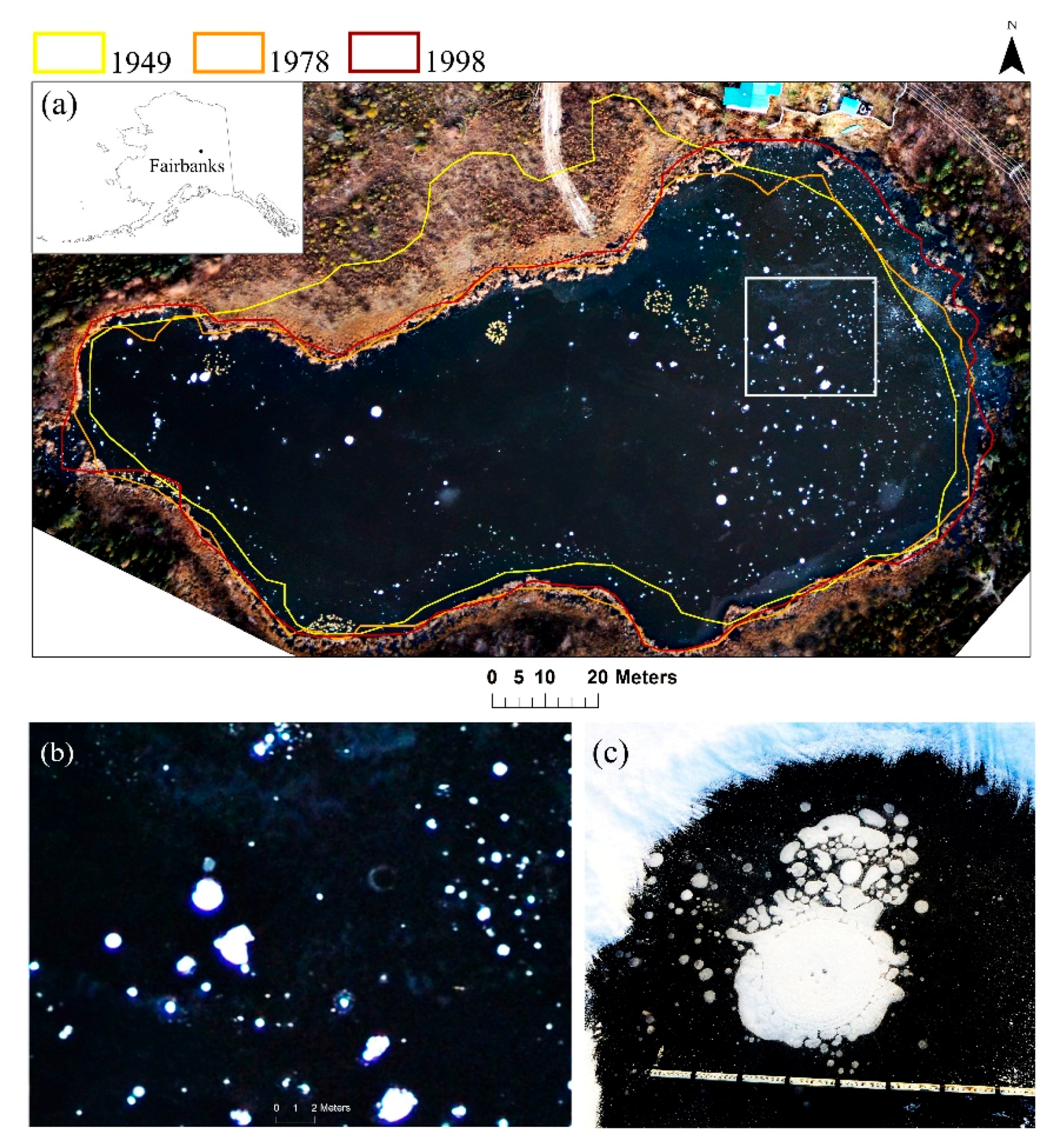
(a) Location of the study area (64.91° N, 147.84° W; 195 m a.s.l.) in Alaska and true color composite of an aerial image of Goldstream Lake, Fairbanks, AK, USA photographed from a fixed-wing airplane using a Nikon D300 photo camera on 13 October 2012. The yellow (1949 shoreline), orange (1978 shoreline) and red (1998 shoreline) polygons overlaid on the 2012 aerial image show the changing shoreline of the lake since 1949. (b) A closer view of lake ice (outlined as white box in the lake image a) shows the appearance of ebullition bubble patches as bright white spots on the aerial image. (c) is an example of methane ebullitions bubbles trapped in lake ice as seen on ground (measurement stick with 10 cm intervals for scale).
Figure 1.
(a) Location of the study area (64.91° N, 147.84° W; 195 m a.s.l.) in Alaska and true color composite of an aerial image of Goldstream Lake, Fairbanks, AK, USA photographed from a fixed-wing airplane using a Nikon D300 photo camera on 13 October 2012. The yellow (1949 shoreline), orange (1978 shoreline) and red (1998 shoreline) polygons overlaid on the 2012 aerial image show the changing shoreline of the lake since 1949. (b) A closer view of lake ice (outlined as white box in the lake image a) shows the appearance of ebullition bubble patches as bright white spots on the aerial image. (c) is an example of methane ebullitions bubbles trapped in lake ice as seen on ground (measurement stick with 10 cm intervals for scale).

Figure 2.
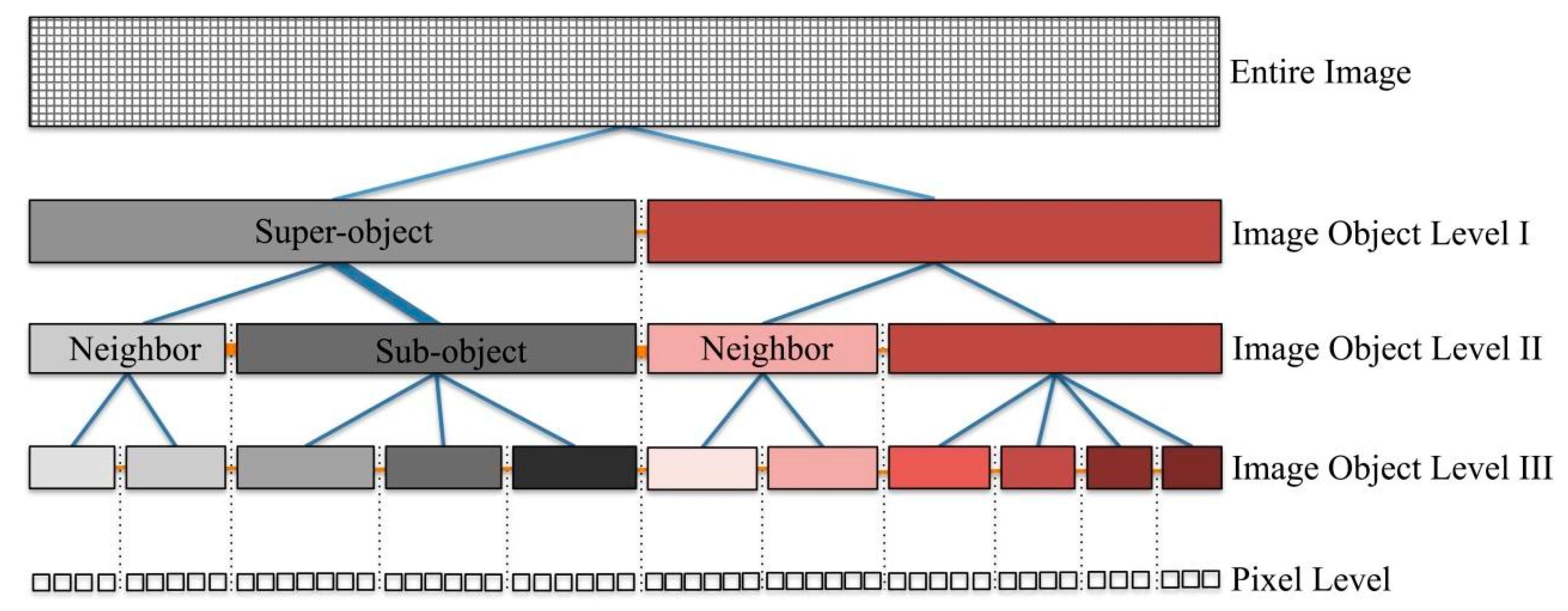
Schematic diagram showing links between image objects in OBIA [19,20]. Objects on the same level are ‘neighbors’, at the upper level they are ‘super-objects’, and at the lower level they are ‘sub-objects’. The horizontal lines (orange) show links between example image objects at the same level (neighbors) and the vertical lines (blue) show links at different levels (super- or sub-object). An image is segmented into appropriate image objects at different levels and classified by assigning each object to a class based on features and criteria set by the user.
Figure 2.
Schematic diagram showing links between image objects in OBIA [19,20]. Objects on the same level are ‘neighbors’, at the upper level they are ‘super-objects’, and at the lower level they are ‘sub-objects’. The horizontal lines (orange) show links between example image objects at the same level (neighbors) and the vertical lines (blue) show links at different levels (super- or sub-object). An image is segmented into appropriate image objects at different levels and classified by assigning each object to a class based on features and criteria set by the user.

Figure 3.
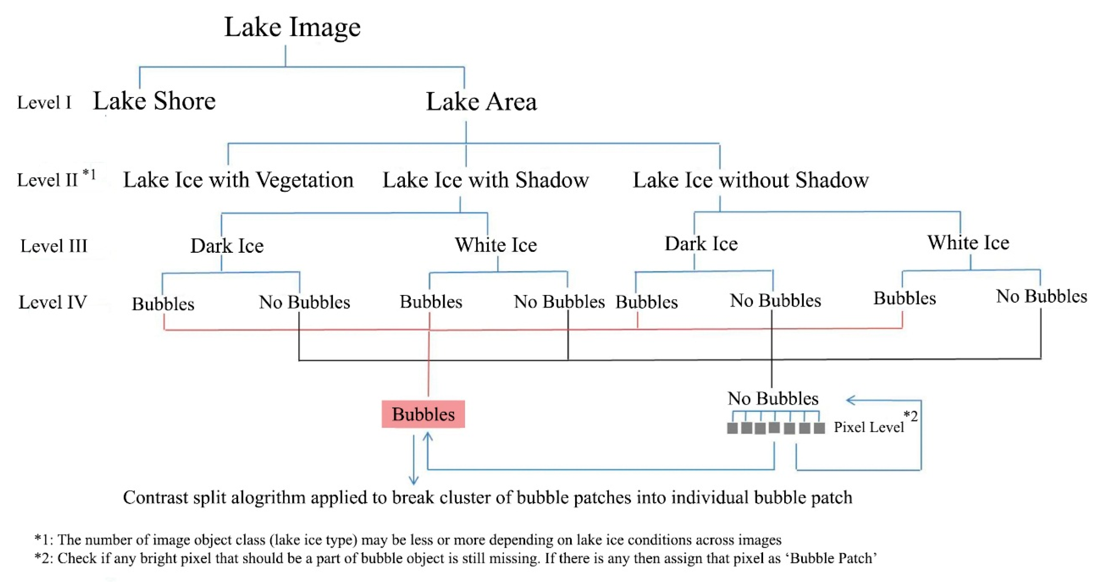
Image object hierarchy to identify ebullition bubble patches on early winter lake ice.

Figure 4.
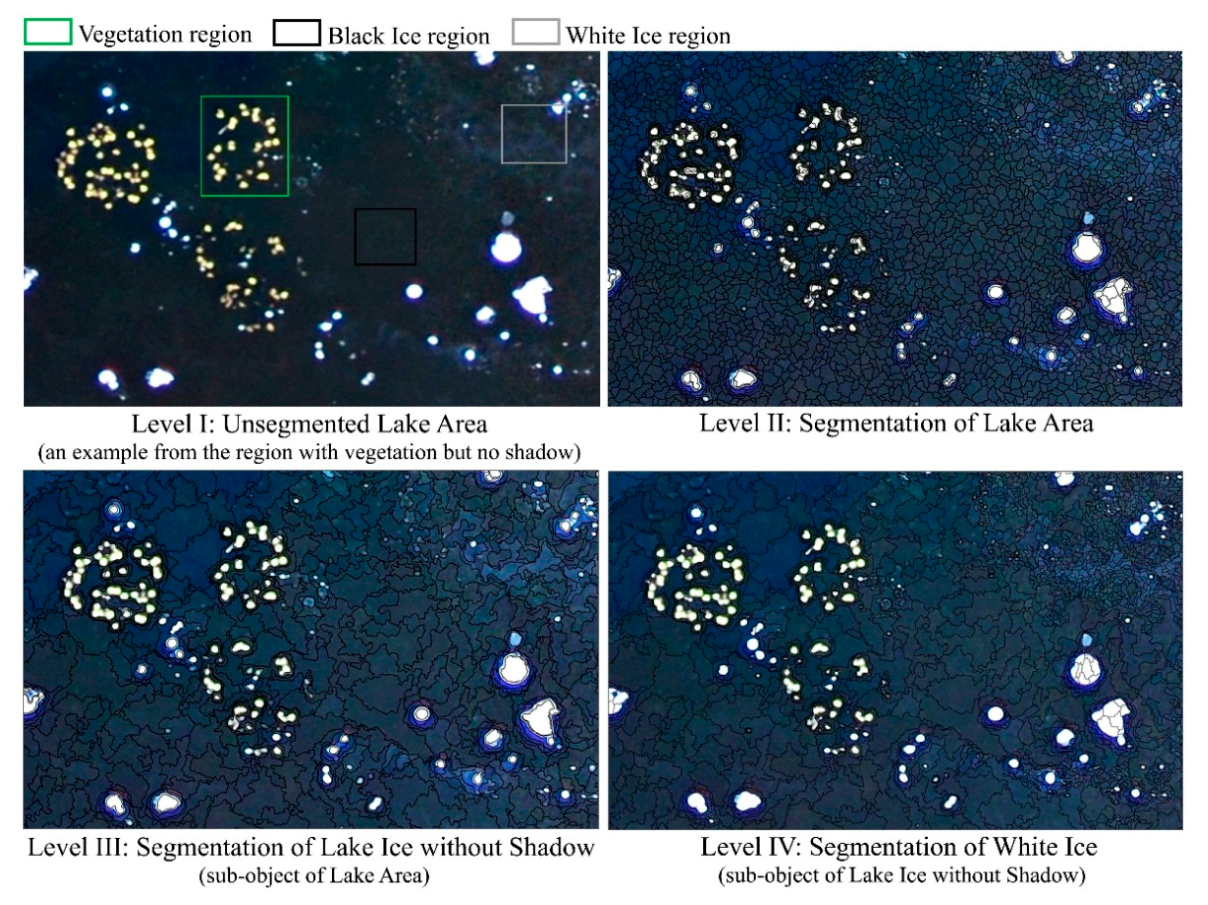
Multiresolution segmentation results show transition of target image objects in terms of shape and size from one level to another. The entire lake area comprised of vegetation, dark, and white ice is segmented (scale factor = 15) in Level II to separate these sub regions. In Level III, only the region with lake ice without shadow comprised of dark and white ice is segmented (scale factor = 50) and only white ice is segmented (scale factor = 10) in Level IV.
Figure 4.
Multiresolution segmentation results show transition of target image objects in terms of shape and size from one level to another. The entire lake area comprised of vegetation, dark, and white ice is segmented (scale factor = 15) in Level II to separate these sub regions. In Level III, only the region with lake ice without shadow comprised of dark and white ice is segmented (scale factor = 50) and only white ice is segmented (scale factor = 10) in Level IV.

Figure 5.
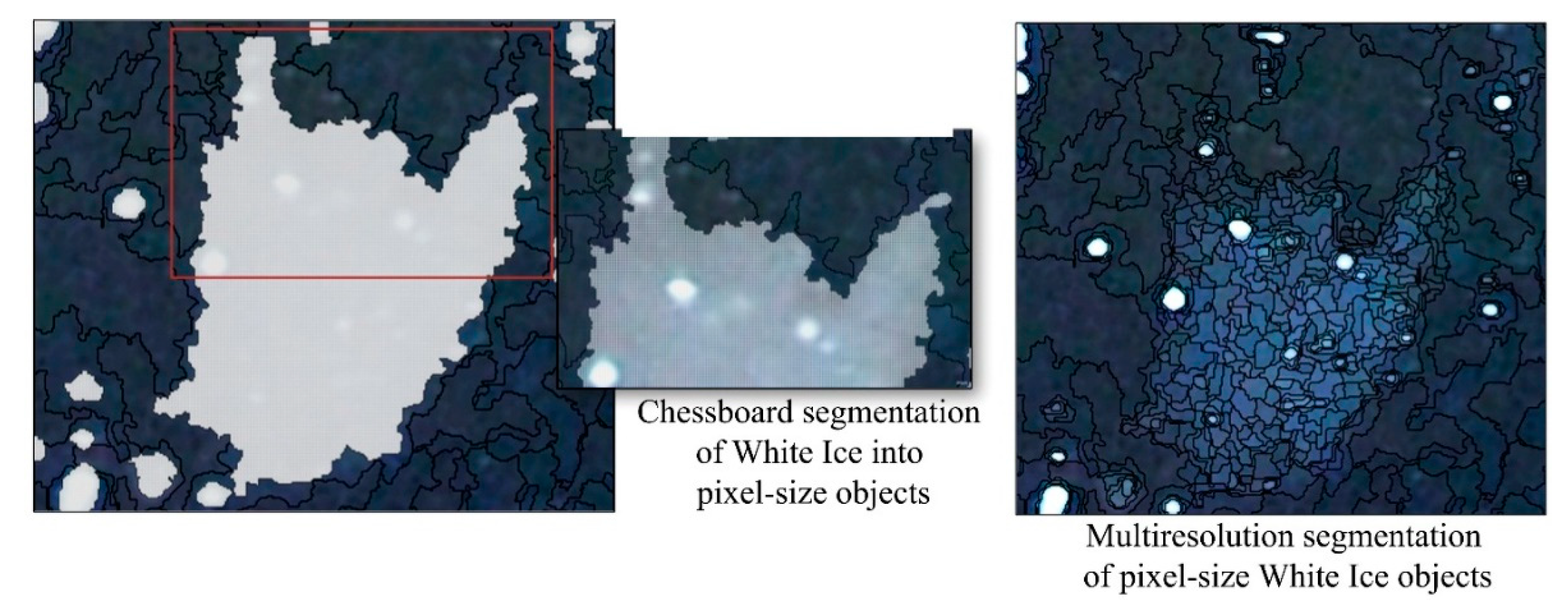
An example of chessboard segmentation to create pixel-size objects followed by multiresolution segmentation on White Ice image objects to identify bubble patches within the white ice region.
Figure 5.
An example of chessboard segmentation to create pixel-size objects followed by multiresolution segmentation on White Ice image objects to identify bubble patches within the white ice region.

Figure 6.
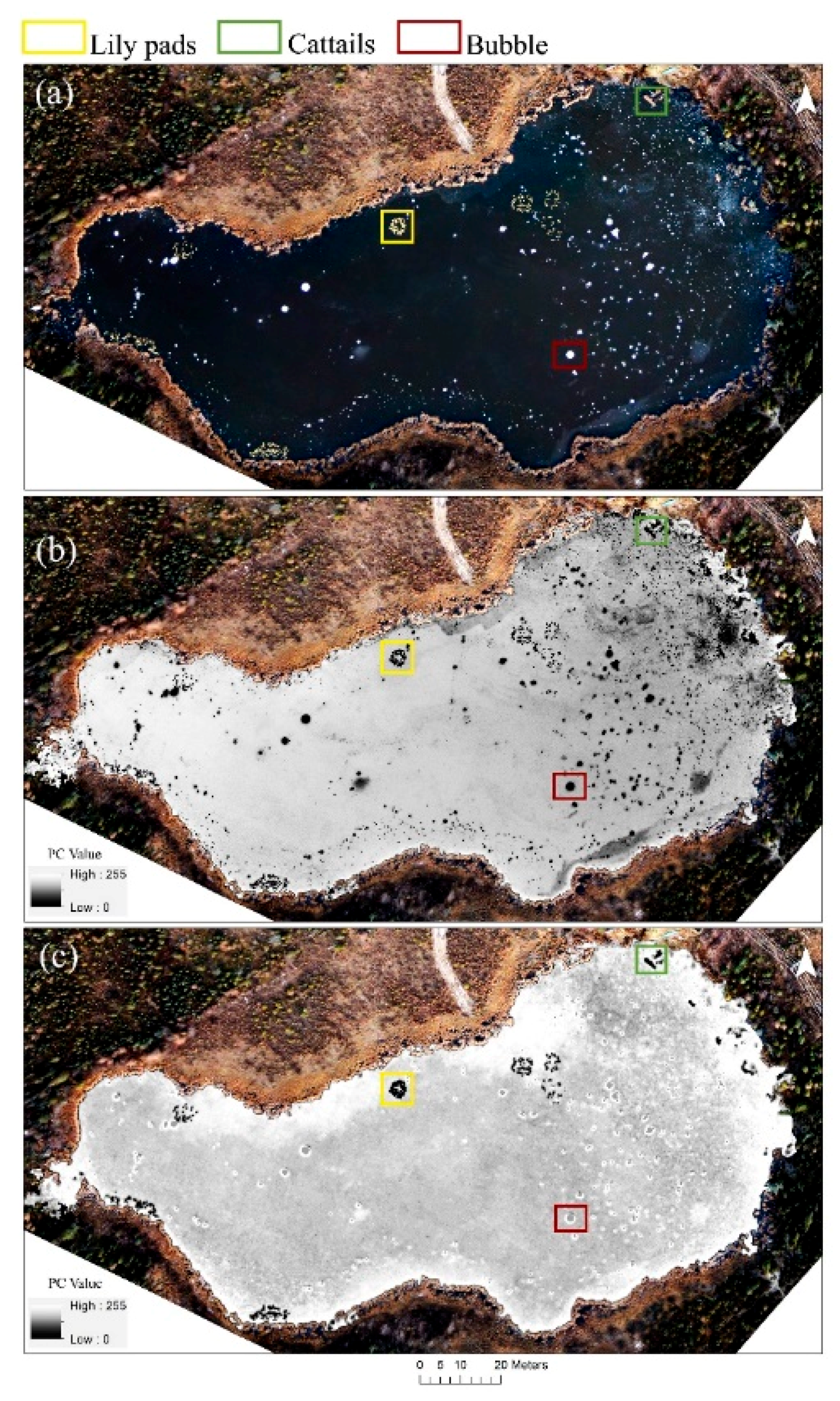
(a) True color composite of aerial image of Goldstream Lake (64.91° N, 147.84° W), Fairbanks acquired on 13 October 2012. (b) PC 1 band of image shown in (a). Bubble patches that appear bright in true color composite in (a) have very low gray values in PC 1 band. The area highlighted in red box is an example. Vegetation such as a cluster of lily pad (yellow box) or cattails (green box) also appears dark in PC 1 band. (c) PC 2 band of image shown in (a). Vegetation is separable from bubble patches. Bubble patches have higher gray values compared to vegetation and appear gray (note: The land area around the lake in (b) and (c) is shown in the true color composite).
Figure 6.
(a) True color composite of aerial image of Goldstream Lake (64.91° N, 147.84° W), Fairbanks acquired on 13 October 2012. (b) PC 1 band of image shown in (a). Bubble patches that appear bright in true color composite in (a) have very low gray values in PC 1 band. The area highlighted in red box is an example. Vegetation such as a cluster of lily pad (yellow box) or cattails (green box) also appears dark in PC 1 band. (c) PC 2 band of image shown in (a). Vegetation is separable from bubble patches. Bubble patches have higher gray values compared to vegetation and appear gray (note: The land area around the lake in (b) and (c) is shown in the true color composite).

Figure 7.
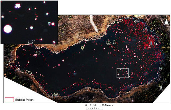
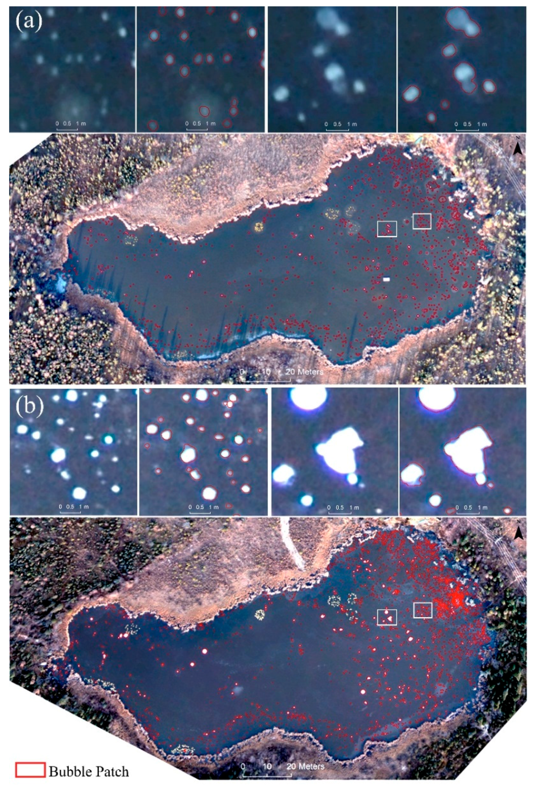
Bubble patch map of Goldstream Lake (64.91° N, 147.84° W), Fairbanks overlaid on true color composite of aerial image acquired on (a) 14 October 2012 and (b) 13 October 2012. The areas outlined in white boxes are zoomed on the top of respective images.
Figure 7.
Bubble patch map of Goldstream Lake (64.91° N, 147.84° W), Fairbanks overlaid on true color composite of aerial image acquired on (a) 14 October 2012 and (b) 13 October 2012. The areas outlined in white boxes are zoomed on the top of respective images.


Table 1.
List of aerial images of Goldstream Lake, Fairbanks.
| Imagery | Scale | Ground Sampling Distance | Date/Year |
|---|---|---|---|
| Aerial imagery (Nikon D300 photo camera) | 1:20,000 | 11 cm | 14 October 2011 |
| Aerial imagery (Nikon D300 photo camera) | 1:17,000 | 9 cm | 13 October 2012 |
| Aerial imagery (digital orthophoto quarter quadrangle (DOQQ), USGS) | NA | 1 m | 2007 |
© 2019 by the authors. Licensee MDPI, Basel, Switzerland. This article is an open access article distributed under the terms and conditions of the Creative Commons Attribution (CC BY) license (http://creativecommons.org/licenses/by/4.0/).
Share and Cite
MDPI and ACS Style
Lindgren, P.; Grosse, G.; Meyer, F.J.; Anthony, K.W. An Object-Based Classification Method to Detect Methane Ebullition Bubbles in Early Winter Lake Ice. Remote Sens. 2019, 11, 822. https://0-doi-org.brum.beds.ac.uk/10.3390/rs11070822
AMA Style
Lindgren P, Grosse G, Meyer FJ, Anthony KW. An Object-Based Classification Method to Detect Methane Ebullition Bubbles in Early Winter Lake Ice. Remote Sensing. 2019; 11(7):822. https://0-doi-org.brum.beds.ac.uk/10.3390/rs11070822
Chicago/Turabian StyleLindgren, Prajna, Guido Grosse, Franz J. Meyer, and Katey Walter Anthony. 2019. "An Object-Based Classification Method to Detect Methane Ebullition Bubbles in Early Winter Lake Ice" Remote Sensing 11, no. 7: 822. https://0-doi-org.brum.beds.ac.uk/10.3390/rs11070822
Note that from the first issue of 2016, this journal uses article numbers instead of page numbers. See further details here.