Hyperspectral Image Classification Based on Fusion of Curvature Filter and Domain Transform Recursive Filter


1
College of Information and Communication Engineering, Harbin Engineering University, Harbin 150001, China
2
College of Rail Transit, Guangdong Communication Polytechnic, Guangzhou 510650, China
*
Author to whom correspondence should be addressed.
Remote Sens. 2019, 11(7), 833; https://0-doi-org.brum.beds.ac.uk/10.3390/rs11070833
Submission received: 21 February 2019
/
Revised: 1 April 2019
/
Accepted: 2 April 2019
/
Published: 7 April 2019
(This article belongs to the Special Issue Image Processing and Analysis: Trends in Registration, Data Fusion, 3D Reconstruction and Change Detection)
Abstract
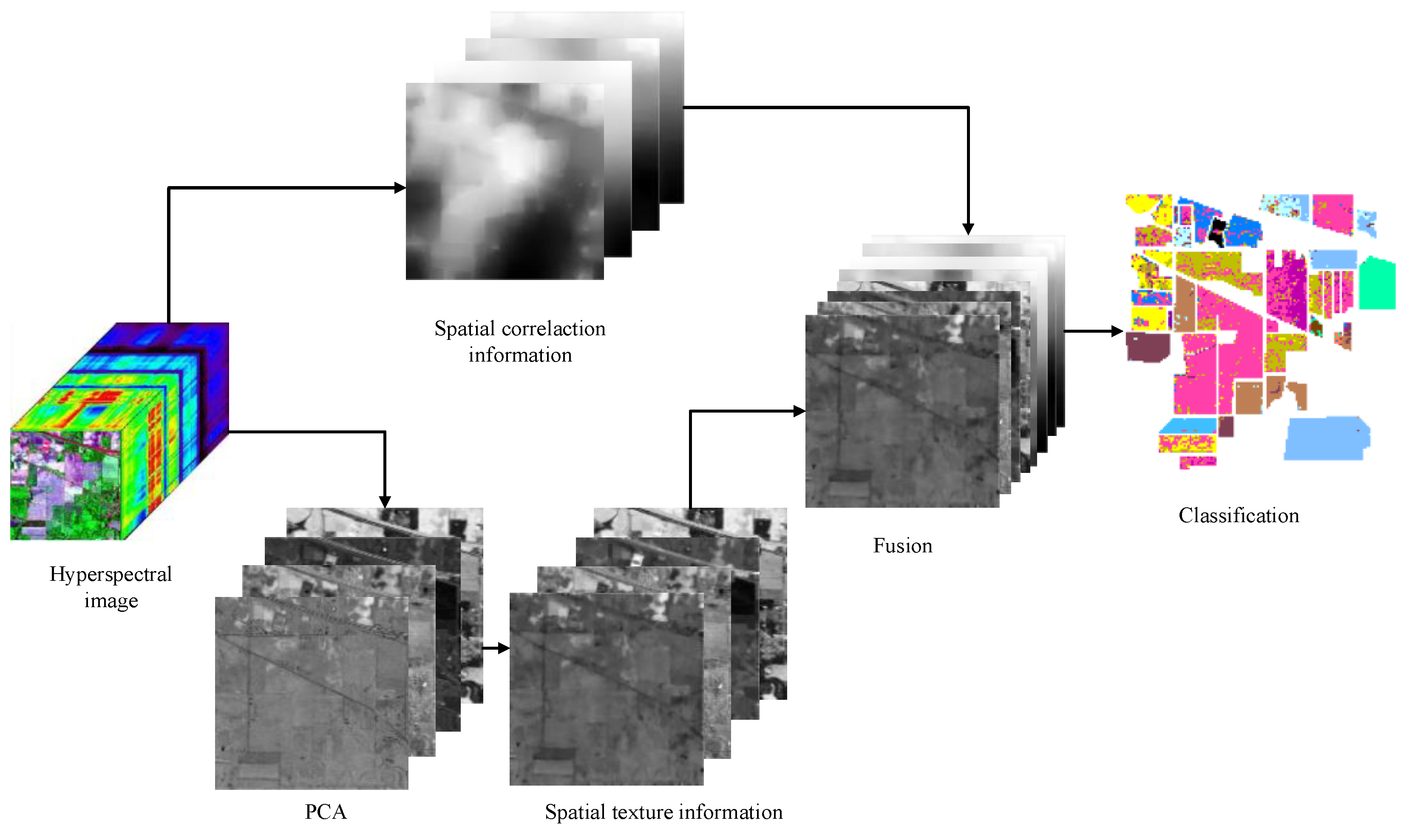
:In recent decades, in order to enhance the performance of hyperspectral image classification, the spatial information of hyperspectral image obtained by various methods has become a research hotspot. For this work, it proposes a new classification method based on the fusion of two spatial information, which will be classified by a large margin distribution machine (LDM). First, the spatial texture information is extracted from the top of the principal component analysis for hyperspectral images by a curvature filter (CF). Second, the spatial correlation information of a hyperspectral image is completed by using domain transform recursive filter (DTRF). Last, the spatial texture information and correlation information are fused to be classified with LDM. The experimental results of hyperspectral images classification demonstrate that the proposed curvature filter and domain transform recursive filter with LDM(CFDTRF-LDM) method is superior to other classification methods.
1. Introduction
Hyperspectral images (HSI), which provide valuable spectral information, have been widely used in remote-sensing applications [1,2,3,4,5,6]. In addition, classification of HSI has drawn lots of attention for its importance in crop monitoring [7], environment monitoring [8], forest monitoring [9], mineral identification [10] and forest mapping [11].
Many scholars around the world have successfully studied various classification methods of HSI, including sparse representation-based techniques [12], Bayesian estimation method [13], K-mean [14], maximum likelihood [15], multinomial logistic regression [16] and deep learning [17]. More specifically, Support Vector Machine (SVM) has been fruitfully applied in HSI classification and achieved respectable results [18]. Zhang et al. adopted the idea of maximizing the margin mean and minimizing the margin variance to improve the maximum margin model of SVM, with the suggestion of using large margin distribution machine (LDM) [19]. In addition, Zhan et al. applied LDM to HSI classification [20].
To improve the classification accuracy, many classification methods with spatial information extraction have been successfully investigated. Some scholars have attempted to obtain spatial information by segmentation to improve HSI classification. A classification method based on the construction of a minimum spanning forest from the region markers, which were gained from the initial classification results [21]. Ghamisi et al. proposed a classification method based on two segmentation methods, fractional-order Darwinian particle swarm optimization and mean shift segmentation, and classified the integration of these two methods by SVM [22]. Also, the existing researches acquired spatial information with morphological profile feature. Multiple morphological profiles were proposed for synthesizing the spectral-spatial information extracted from the multicomponent base images and were interpreted with decision fusion and sparse classifier based on multinomial logistic regression [23]. The method proposed by Xue et al. for HSI classification was performed via morphological component analysis-based image separation rationale in sparse representation [24]. Liao et al. applied the morphological profile filter and domain transform normalized convolution Filter (DTNCF) to extract the spatial information [25], which was combined and fed into support vector machine (SVM), and finally implemented two-step optimization in the classification process [26]. Moreover, some scholars attempted to improve classification performance with Markov random field [27]. For instance, Sun et al. proposed an HSI classification method, including a spectral data fidelity term and a spatially adaptive Markov random field prior in the hidden field based on maximum a posteriori framework with sparse multinomial logistic regression [28]. Zhang et al. used an extended Markov random field model to combine the multiple features with local and nonlocal spatial constraints in the semantic space with probabilistic SVM for HSI classification [29].
In order to obtain the fully spatial features of HSI, many classification methods for spatial information extraction have been investigated. For example, the integration of spectral and spatial context was an effective method for HSI classification, and more researchers intended to extract spatial information with different filters, such as guided filter (GDF) [30], bilateral filter (BF) [31], Gabor filter (GF) [32] and etc. Wang et al. suggested a filtering framework named discriminatively guided image filtering which integrates SVM and linear discriminative analysis by GDF to enhance classification performance [33]. A method of k-nearest neighbor with GDF was presented by Guo et al. to extract spatial information and optimize the classification accuracy [34]. WANG et al. proposed a spectral-spatial HSI classification method based on joint BF and graph cut segmentation with the SVM classifier [35]. Sahadevan et al. integrated the spatial texture information obtained with BF into the spectral domain to improve SVM performance [36]. A hyperspectral classification method was proposed based on sparse representation classification spatial features, which were extracted by joint BF with the first principal component as the guidance image in the literature [37]. Edge-preserving filter (EPF) and principal component analysis (PCA) [38]-based EPFs (PCA-EPFs) methods with GDF or BF and recursive filter were adopted to progress SVM classification performance in the references of [39] and [40], respectively. Moreover, a feature extraction method based on the image fusion with multiple subsets of adjacent bands and recursive filter (IFRF) was achieved by Kang et al. to increase accuracy of HSI classification [41]. In addition, a spectral-spatial Gabor surface feature fusion method was completed with including SVM classifier for HSI classification, and the magnitude pictures of Gabor features were extracted by 2 dimensional GF in the reference [42]. Li et al. projected Gabor features of the hyperspectral image obtained with GF into the kernel induced space through composite kernel technique [43]. Chen et al. combined GD with deep convolutional neural networks to mitigate overfitting problem and increase classification accuracy for HSI classification [44]. Tu et al. proposed an HSI classification method o based on non-local means filtering with maximum probability and SVM, which uses the spatial context information and non-local means filtering in the first principal component to obtain the optimization probability image of spatial structure [45].
A filter can be used to extract spatial texture features, but it is difficult to get complete spatial features using a single filter. In this paper, we first used the curvature filter (CF) to extract the spatial texture features [46,47], and then applied DTRF [25] to attain spatial correlation features to enrich the spatial characteristics and provide more effectively hyperspectral image classification. Finally, LDM can be adopted to classify the fusion of two spatial information to form a new classification method, which combine the curvature filter and domain transform recursive filter with LDM (CFDTRF-LDM). The work of this paper can be summarized as follows:
- (1)
- CF with the minimal projection operator has superior characteristics of small calculation amounts and fast convergence [46], which can efficiently extract the spatial features of a hyperspectral image. The spatial correlation information of obtained by DTRF benefits the spatial texture information to improve classification accuracy.
- (2)
- The effective fusion of the two spatial information is conducive to the LDM classification and is superior to other methods.
2. Methodology
2.1. Classification Method for HSI
LDM improves the SVM classification performance with simultaneous maximization of the margin means and minimization of the margin variances. A training set is defined as , in which, xi is the training sample labelled by , and m is the number of the training data. The function of SVM was to predict the unlabeled data with the hyperplane of maximization of the minimum margin [48], and can be shown as follows:
where is the weight vector of decision function, is the linear model and is a mapping of by a kernel k, such as:
The margin of instance can be formulated as
For the inseparable conditions, the soft-margin LDM can be expressed as Equation (4).
where and are the parameters corresponding to the trading-off the margin variance and the margin mean. The margin mean and the margin variance can be characterized as Equations (5) and (6), respectively.
2.2. Spatial Information Extraction
In order to obtain fully spatial information, CF and DTRF were used to extract the spatial texture features and spatial correlation features, and the principle of the CF and DTRF will be analyzed in the following.
2.2.1. Curvature Filter
Curvature filter is proposed to first study the surface corresponding to the curvature and then select one of all surfaces to best approximate the data. As a unique optimization algorithm, the curvature filter optimizes regularization energy and implicitly uses known differential geometry surfaces in the filtering process.
A. Optimization of energy functional
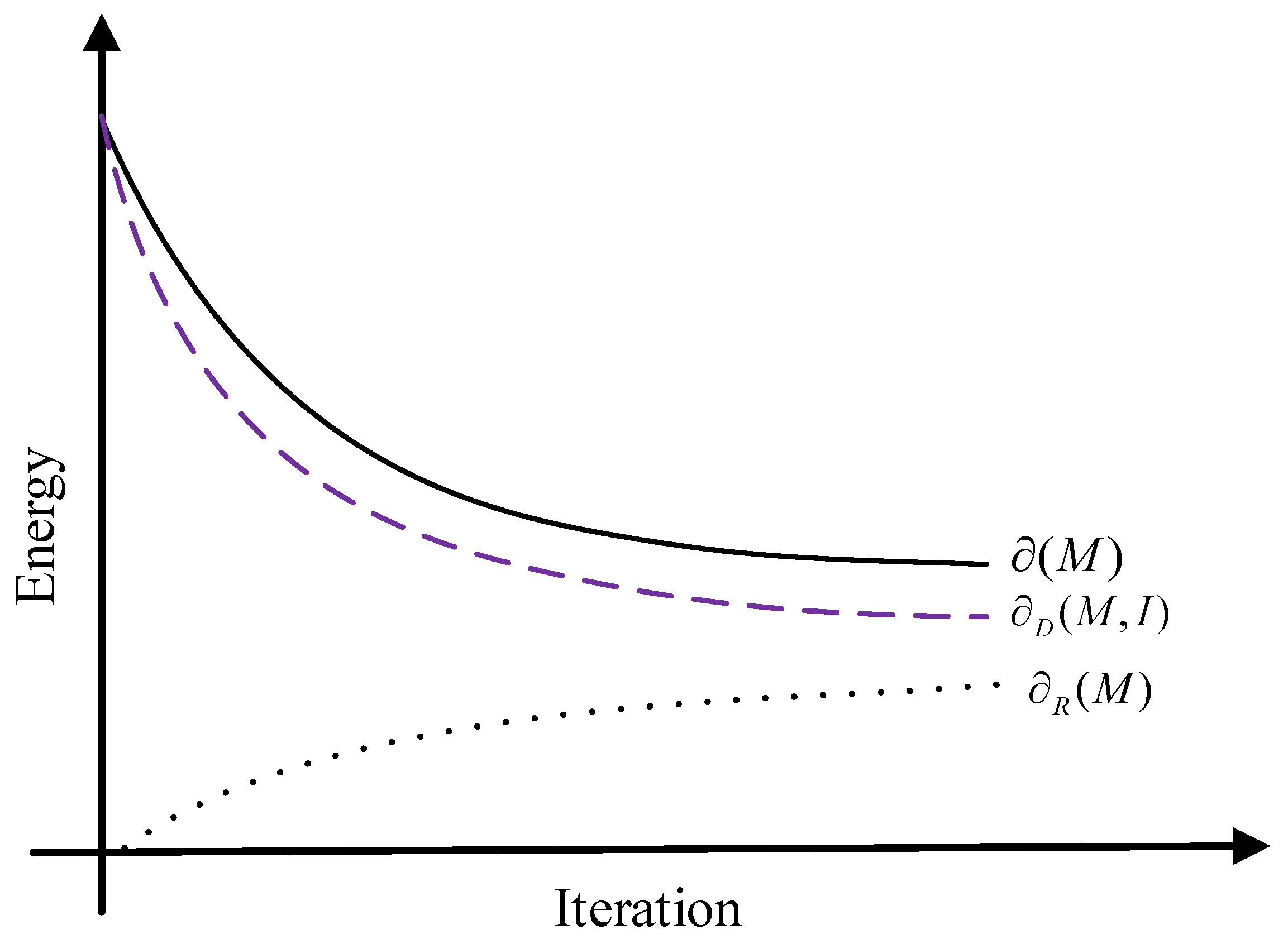
The basic idea of the variational regularization method is to first define the energy function of the image processing problem. When the energy function is smaller, the variable is closer to the expected result. There is a relationship in the process of optimizing the model
where , which is data-fitting energy, measured how well fits the image data . that is regularization energy formalized prior knowledge about , and is scalar regularization coefficient used to measure the contribution of the two energy.
The evolution process of the energy function in the variational model is shown in Figure 1. The data-fitting energy is always increasing, while the regular energy is decreasing. Since the overall energy is decreasing, this indicated that the regularization energy is the main part in the optimization process. Therefore, curvature filtering suggests optimizing the regular energy. As long as the reduction of the regular energy is greater than the increase in the data-fitting energy, the overall energy decline can be guaranteed. The curvature filter proposes to optimize the variational model, which is to reduce the energy of the curvature regular energy to a minimum value, and minimize the regular energy by minimizing the regular curvature from the perspective of differential geometry [46].
B. Domain decomposition
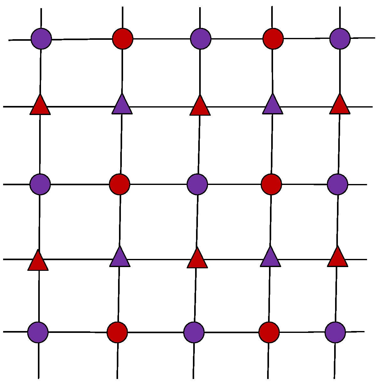
There is a dependency between adjacent pixels, which hinders local minimization of the principal curvature. A domain decomposition algorithm was proposed here to circumvent the problem.
As shown in Figure 2, the discrete domain Ω of image U was decomposed into four subsets: red triangle RT, red circle RC, purple triangle PT, purple circle PC. The advantages of this decomposition were as follows: (1) the dependence of adjacent pixels can be eliminated, and the filtering efficiency can be improved; (2) the updated field can be used to ensure convergence due to independence; (3) all the tangent planes can be enumerated in a 3 × 3 local window [46].
C. Projection to the tangent plane
Assuming that a pixel is , constructing the surface is to project the current pixel value of hyperspectral image onto the ideal pixel value which is on the optimal tangent plane of the adjacent pixel [46]. The relationships are met as following:
where is the projection distance.
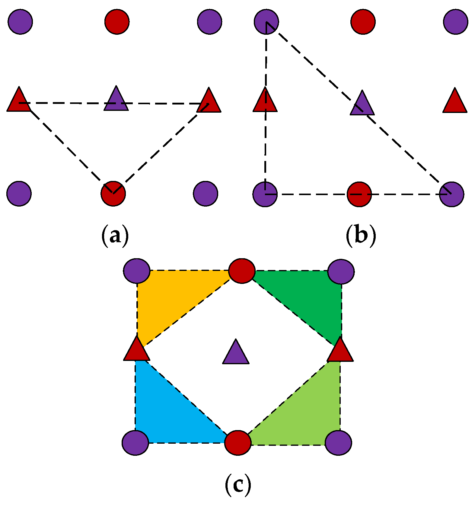
To find the optimal tangent plane of the field , all possible triangles are enumerated in the 3 × 3 neighborhood of x (as shown in Figure 3, excluding x as the vertex). Among them, four pass the red field R, and four pass the purple field P, and four pass the red/purple mixed field RP.
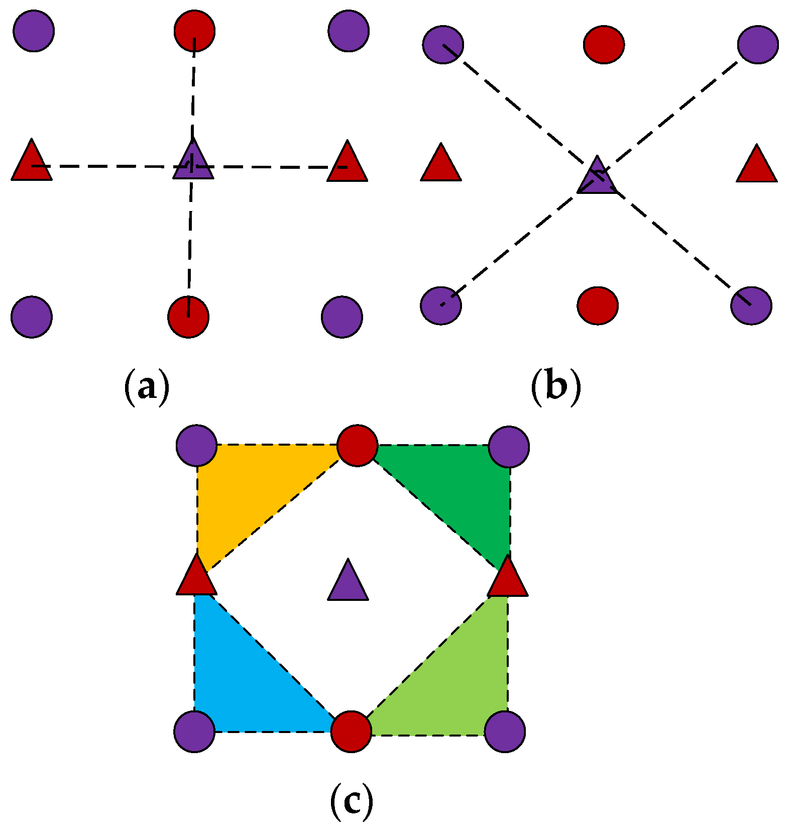
As shown in Figure 4, since there are common edges of passing through the 12 triangular sections and the projection was sufficient, there were only eight different projection distance . There are two common edges in R, two common edges in P, and four mixed tangent planes.
D. Minimal Projection Operator (Pg)
According to Euler’s theorem, it can be known that:
where: , are the principal curvatures; is the angle to the principal plane. If the angular sample is sufficiently dense within (), when , there is dm ≈ min{ki}.
For the pixel at (i, j), the distance dm can be obtained from the tangent plane with the neighborhood pixels in the 3 × 3 window [46].
Therefore, the minimum absolute value dm is taken as the minimum projection of to .
is on the tangent plane of the field
E. Gaussian curvature filter
The minimum projection operator is iterated with all pixels of , , and , and the Gaussian curvature filter can be generated as:
As a unique optimization algorithm, Gaussian curvature filtering is an image smoothing algorithm with edge protection, which assumes that the surface formed by the ideal noise-free image is block-expandable, and the Gaussian curvature is zero everywhere. Also, the pixel values are directly adjusted so that the tangential plane of the domain pixel satisfied the assumption, avoiding the explicit calculation of the Gaussian curvature. Thus, the image surface is no longer required to have second-order variability, allowing for the presence of abrupt edges and corners in the image to ideally protect the edges of image.
In hyperspectral images, there are hundreds of frequency bands, high correlation between large amount of data and adjacent bands, which leads to redundant information. In order to obtain more comprehensive spatial information with CF, we first use PCA to reduce dimensionality of hyperspectral images. The CF validation test will be found in Section 3.3.
2.2.2. Domain Transform Recursive Filter (DTRF)
DTRF proposed by Gastal et al. is used for image filtering, in which two-dimensional image filtering can be converted into one-dimensional image filtering [25]. The energy function of DTRF for hyperspectral image R at the i-th band can be represented as:
and
where is a feedback coefficient, is the hyperspectral image, is the result of the (n-1)-th recursive filtering, is the distance between neighbor samples and in the transformed domain , which is calculated by integrating the partial differential for the hyperspectral band image , which is transformed into an increasing function. Besides, is filter radius, is the spatial standard deviation, is the range standard deviation, is the value of the t-th iteration, and is the total number of iterations.
DTRF has an infinite impulse response with the exponential decay. Briefly, as increases, goes to zero, which stops the propagation chain, indicating that the neighborhood pixels are in the same ground. Equation (14) is an asymmetric causal filter and depended on input and output information. To obtain the filtering symmetry, this equation needs to be executed twice, such as the procedures: first from left to right, and then from right to left; or from top to bottom, and then from bottom to top [25].
In general, the ground distribution of hyperspectral images has suitable uniformity, so there is always a strong spatial correlation between pixels in a hyperspectral image. Moreover, the spatial correlation meaning is an associated property of the reflection intensity between a pixel and an adjacent pixel. However, spatial correlation information is often ignored in texture information extraction.
To examine the spatial correlation features of CF and DTRF, Moran’s I [49,50] is employed to test the spatial correlation of hyperspectral images before and after filtering, calculated by the following formula:
where and are the reflection intensities of two hyperspectral pixels, and is the average of . n is the pixel number of one band, and is the spatial weight.
The larger I is larger, the stronger the spatial correlation and vice versa. Section 3.4 describes validation tests for spatial correlation information extraction with DTRF.
2.3. CFDTRF-LDM
Based on CF and DTRF, a new classification approach (CFDTRF-LDM) is proposed. CF and DTRF are respectively applied to extract spatial texture information and spatial correlation information. In order to obtain rich spatial correlation feature, the spatial correlation information is obtained from original spectral images. In addition, in order to avoid the hughes phenomenon, the spatial correlation information and spatial texture information were obtained from the original image and the components of PCA respectively, so the total numbers of images are suitable for LDM classification. The implementation process will be depicted as following.
Step 1: normalization. The formula (21) normalized the hyperspectral image R, where and are corresponding to the mean and standard deviation of R.
Step 2: dimensionality reduction. Since most of the information is distributed in the front principal component after the PCA dimension is reduced, the normalized image H will be further lowered by PCA, while the top 10% of the principal componentis selected for CF.
Step 3: spatial texture information extraction. CF extracts the spatial texture information on each band of E by Equation (13).
Step 4: spatial correlation information extraction. DTRF extracts the spatial correlation information from .
Step 5: fusion. Equation (23) linearly fuses and :
Step 6: classification. The training set is randomly selected in proportion from D and the test set is formed with the remaining samples, which is verified by the LDM classifier.
The flow of the CFDTRF-LDM is shown in Figure 5.
3. Experiments
3.1. Hyperspectral Data Description
Three hyperspectral image datasets were used to verify the effectiveness of CFDTRF-LDM. The first dataset was Indian Pines [51], which was acquired in 1992 by the airborne visible infrared imaging spectrometer (AVIRIS) sensor in the Indian Pines region of Northwestern Indiana. It contains 220 spectral bands with a spatial size of pixels. Due to noise and water absorption, 20 spectral bands were removed, leaving 200 bands remaining. This image includes 16 classes, and the specific types and the numbers of each class are shown in Table 1.
The second dataset was Salinas Valley [52] collected by AVIRIS in the Salinas Valley, Southern California, in 1998. It has a high spatial resolution of 3.7 m with a region of the spatial size of pixels and 206 spectral bands. Similarly, 200 bands were retained because of noise and water absorption. The image also includes 16 classes, and the specific types and numbers of each class are shown in Table 2.
The third dataset was Kennedy Space Center acquired by NASA airborne visible/infrared imaging spectrometer (AVIRIS) at the Kennedy Space Center in Florida on 23 March 1996. AVIRIS collected 224 bands with 10 nm width with the center wavelengths from 400–2500 nm. The Kennedy Space Center dataset was available at an altitude of approximately 20 km with a spatial resolution of 18 m. After removal of water absorption and low SNR bands, 176 bands were used for the analysis. The image also includes 13 classes, and the specific types and numbers of each class are shown in Table 3.
3.2. Parameter Setting
To demonstrate the superiority of the proposed method, several methods were used to compare with CFDTRF-LDM, including:
- (1)
- SVM [18]: according to the raw features of hyperspectral images, SVM was applied with the Gaussian radial basis function kernel.
- (2)
- PCA-SVM (PCA with SVM): the use of PCA reduced the hyperspectral dimension and selected the top 10% components for the SVM.
- (3)
- LDM: gaussian radial basis function kernel was applied according to the raw features of hyperspectral images.
- (4)
- PCA-LDM (PCA with LDM): PCA reduced the hyperspectral dimension and selected the top 10% components for the LDM.
- (5)
- EPF [39]: in this method, SVM classified hyperspectral images. Next, edge-preserving filter was conducted for each probabilistic map. Last, the class of every pixel was selected based on the maximum probability.
- (6)
- IFRF [41]: this method acquired the classified results with SVM according to the image fusion and recursive filter.
- (7)
- PCA-EPFs [40]: the spatial information constructed by applying edge-preserving filters was stacked to form the fused feature, and the dimension was reduced by PCA for the classifier of SVM.
- (8)
- LDM and feature learning-based(LDM-FL) [20]: this method attained the classified results with LDM from the recursive filter.
- (9)
- CF-SVM: the hyperspectral dimensionality was reduced with PCA, and the first 10% principal components were selected for SVM based on CF.
- (10)
- CF-LDM: the hyperspectral dimensionality was reduced with PCA, and the first 10% principal component were selected for LDM based on CF.
- (11)
- DTRF-SVM: the hyperspectral dimensionality was reduced with PCA, and the first 10% principal components were selected for SVM according to DTRF.
- (12)
- DTRF-LDM: the hyperspectral dimensionality was reduced with PCA, and the first 10% principal components were picked for LDM based on DTRF.
- (13)
- CFDTRF-LDM: the advanced method in this paper.
- (14)
- CFDTRF-SVM: in addition to the classification results, the advanced method was generated by SVM in this paper.
In this paper, overall accuracy (OA), average accuracy (AA) and kappa statistic (Kappa) were adopted to test the classification accuracy. To avoid biased estimation, twelve independent tests were carried out using the computer program of Matlab R2012b based on the configuration of i7-6700 CPU and 8GB RAM.
3.3. The Validation Test of CF and DTRF
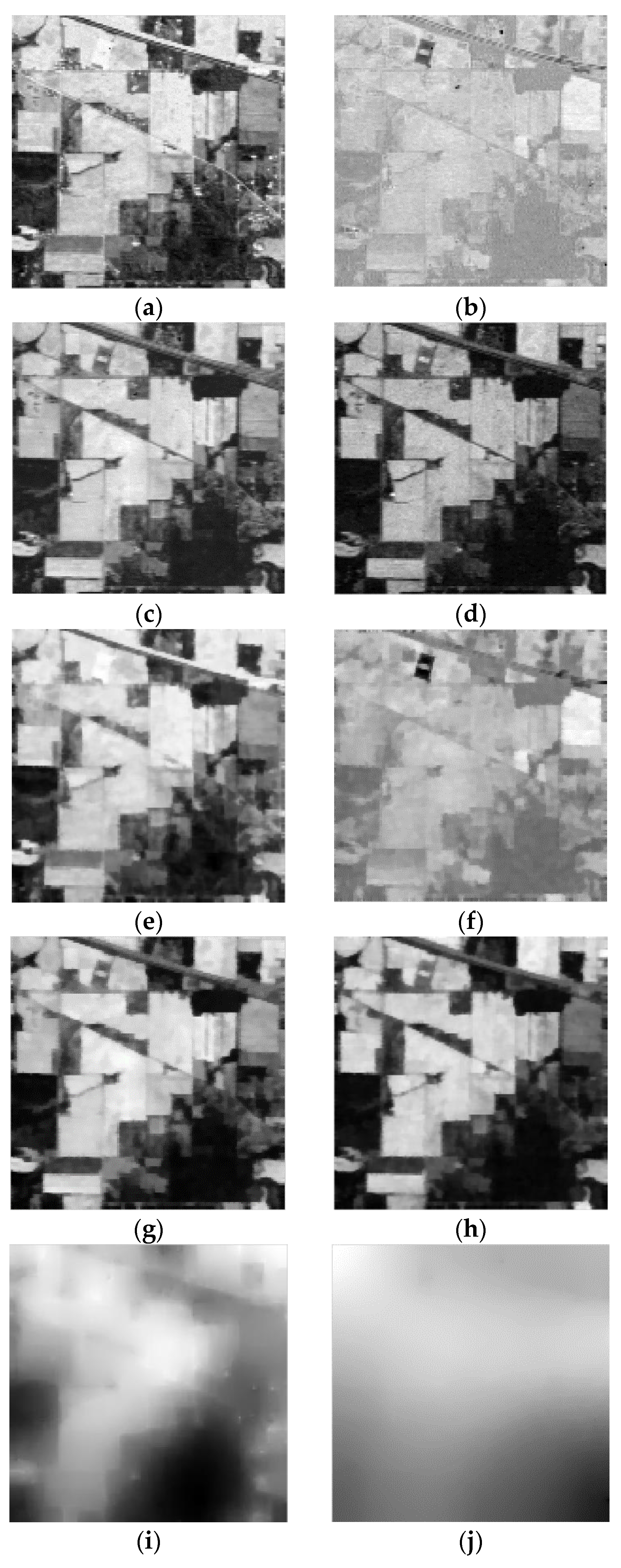
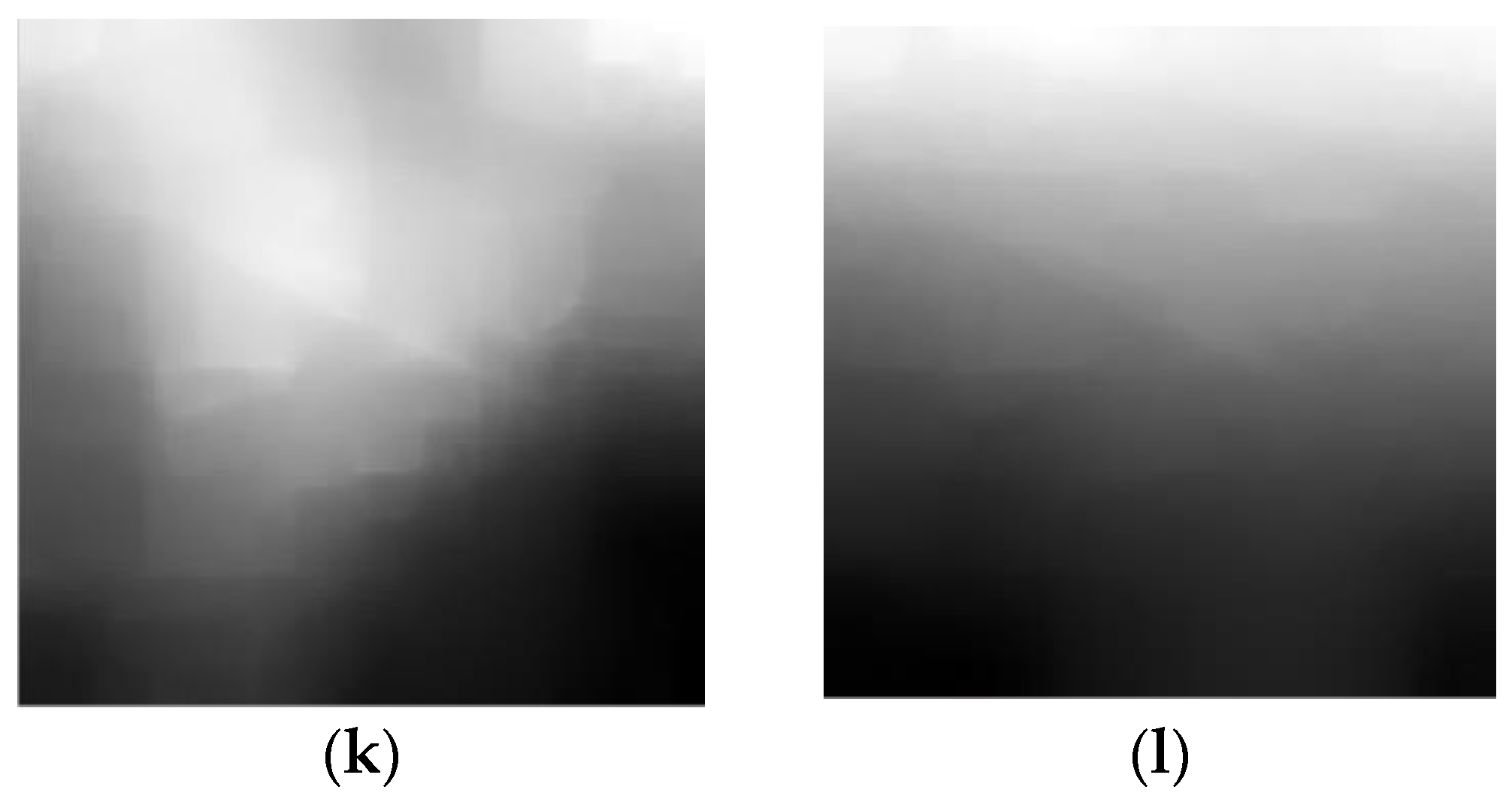
To verify CF validation, the 10th, 60th, 130th and 180th bands of Indian Pines were processed with CF. As shown in Figure 6, CF can extract good boundary features of hyperspectral images, and has great advantages in obtaining smooth edges by using CF smooth hyperspectral images. Also, DTRF owns good spatial correlation preserving characteristics.
3.4. Test of Spatial Correlation Information
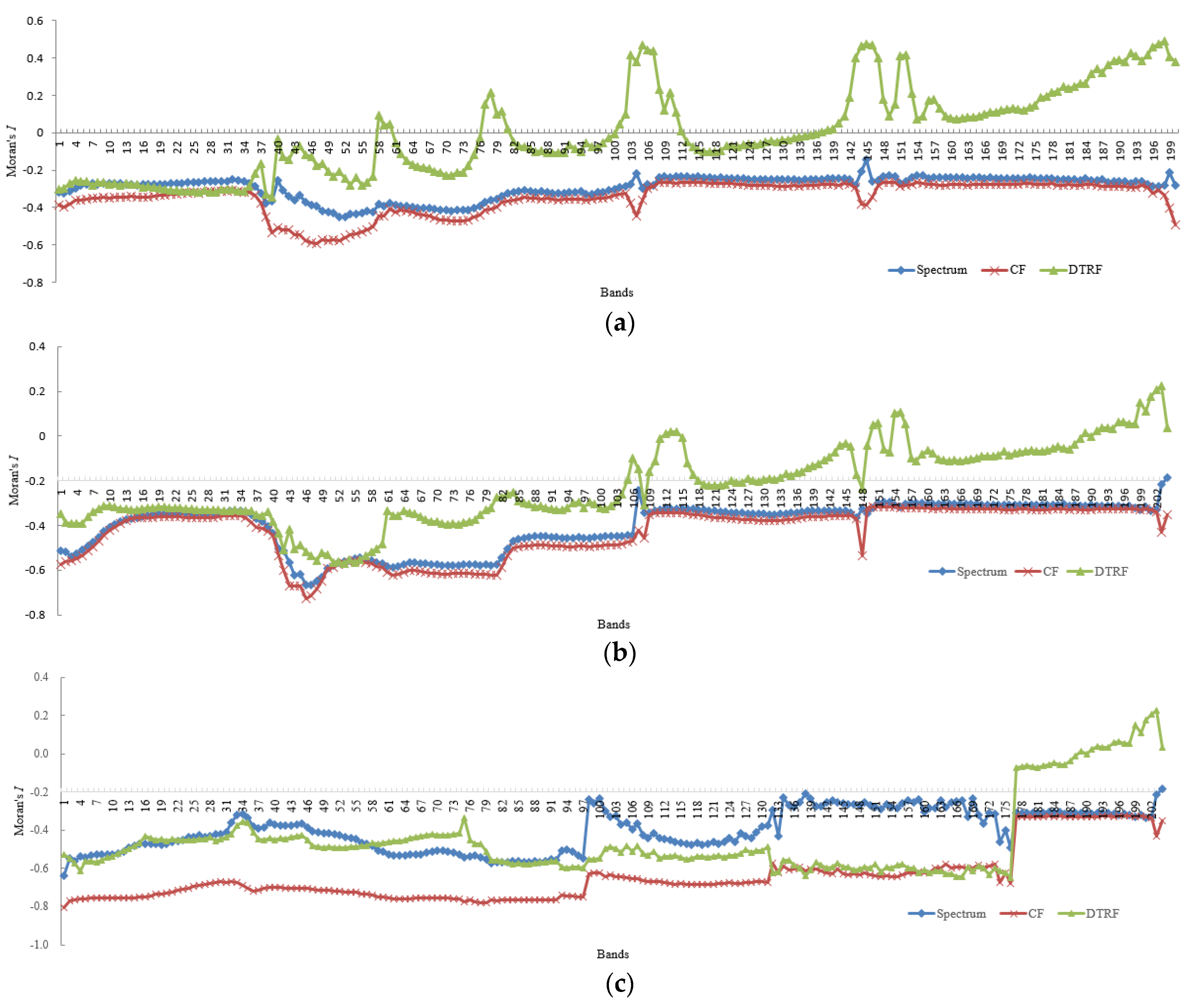
To compare the spatial correlation of CF and DTRF, we calculated the mean of Moran’s I for each band of Indian Pines, Salinas Valley and Kennedy Space Center datasets. The average Moran’s I of the two filters is shown in Figure 7. It can be found that the average of Moran’s I obtained from DTRF is higher than the average of CF and raw spectral features. In addition, the average of Moran’s I acquired by CF is lower than that of the spectrum images, suggesting that the spatial correlation information is weak. Therefore, it can be illustrated that DTRF can extract good spatial correlation information and effectively compensate for the deficiency of CF.
3.5. Investigation of the Proposed Method
3.5.1. Optimization of DTRF
The total number of iteration N, spatial standard deviation and the range standard deviation of DTRF can influence the filtering effect of the image. Therefore, a classification test was conducted for the Indian Pines dataset to verify the effectiveness of parameter optimization. From the entire data set, 4% and 96% of the training and test samples were randomly selected, and the exhaustive method was employed to establish the three optimal parameters to obtain the most satisfactory LDM classification results. To reduce the complexity of the algorithm, we first set the total number of iterations N = 10. Then, and were set for experiments. Last, the experiments were performed sequentially for the classification with 4059 iterations. According to the iteration result, when and , the best classification can be obtained and the optimal OA = 90.23%. Therefore, to achieve a better classification, the parameters of and will be adopted in the following experiments.
3.5.2. Experiment of Indian Pines
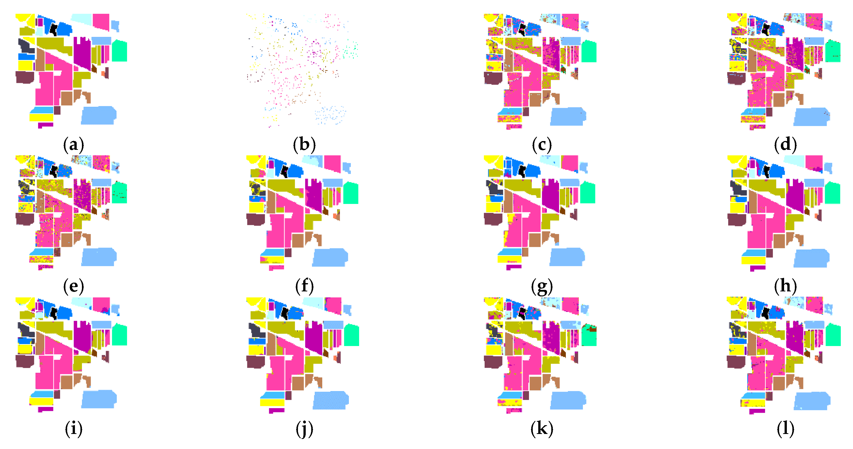
To evaluate the performance of CFDTRF-LDM, fifteen methods were used to classify and validate the data from Indian Pines. The verified method is as follows: The distribution of Indian Pines datasets is shown in Figure 8a. All 16 categories were selected, of which 5% (about 533) samples were employed as the training set with the rest as test set, while 20% of the three types of Indian Pines grounds were insufficient for training. Table 1 and Table 2 shows the classification accuracy generated by fifteen classification methods, as shown in Figure 8.
The classification results for Indian Pines are shown in Figure 8, while Table 1 and Table 2 shows the accuracies of OA, AA and Kappa for each class of the different methods, and also indicates CFDTRF-LDM achieved the best accuracy, when OA = 96.64%, AA = 96.04% and Kappa = 96.18%. Furthermore, the accuracies can be over 99% of six classes for CFDTRF-LDM. This experiment demonstrates that the classification performance was improved compared to other classification methods.
Besides, the OA values of CFDTRF-LDM for Indian Pines are shown in Figure 8, which are 19.17%, 18.83%, 16.78%, 18.15%, 6.29%, 5.99%, 1.85%, 0.60%, 8.55%, 6.99%, 4.34% and 2.04%, correspondingly higher than that of SVM, PCA-SVM, LDM, PCA-LDM, EPF, IFRF, LDM-FL, CF-SVM, CF-LDM and GDF-LDM, DTRF-SVM and DTRF-LDM. The effectiveness of CFDTRF-LDM is fully verified for the hyperspectral classification.
3.5.3. Experiment of Salinas Valley
Similarly, the distribution according to the Salinas Valley dataset is shown in Figure 9a: all 16 classes were selected, with 0.8% (about 433) samples as the training set, and the remaining 99.2% as the test set. Table 2 lists the classification accuracy of the Salinas Valley dataset for different methods. The classification effects are shown in Figure 9.
The classification results for Salinas Valley are shown in Figure 9, while Table 3 and Table 4 shows the accuracies of OA, AA and Kappa for each class of the different methods, and also indicates CFDTRF-LDM achieved the best accuracy, when OA = 99.16%, AA = 98.71% and Kappa = 99.06%. Furthermore, the accuracies reached 100% of four classes for CFDTRF-LDM. This experiment demonstrates that the classification performance was improved compared to other classification methods.
In addition, the OA values of CFDTRF-LDM were higher than that of SVM, PCA-SVM, LDM, PCA-LDM, EPF, IFRF, LDM-FL, CF-SVM, CF-LDM, GDF-LDM, DTRF-SVM and DTRF-LDM by 11.17%, 11.71%, 10.20%, 9.97%, 7.79%, 1.64%, 0.48%, 0.40%, 9.96%, 6.56%, 2.45% and 0.64%, respectively. The hyperspectral classification fully validated the effectiveness of CFDTRF-LDM.
3.5.4. Experiment of Kennedy Space Center
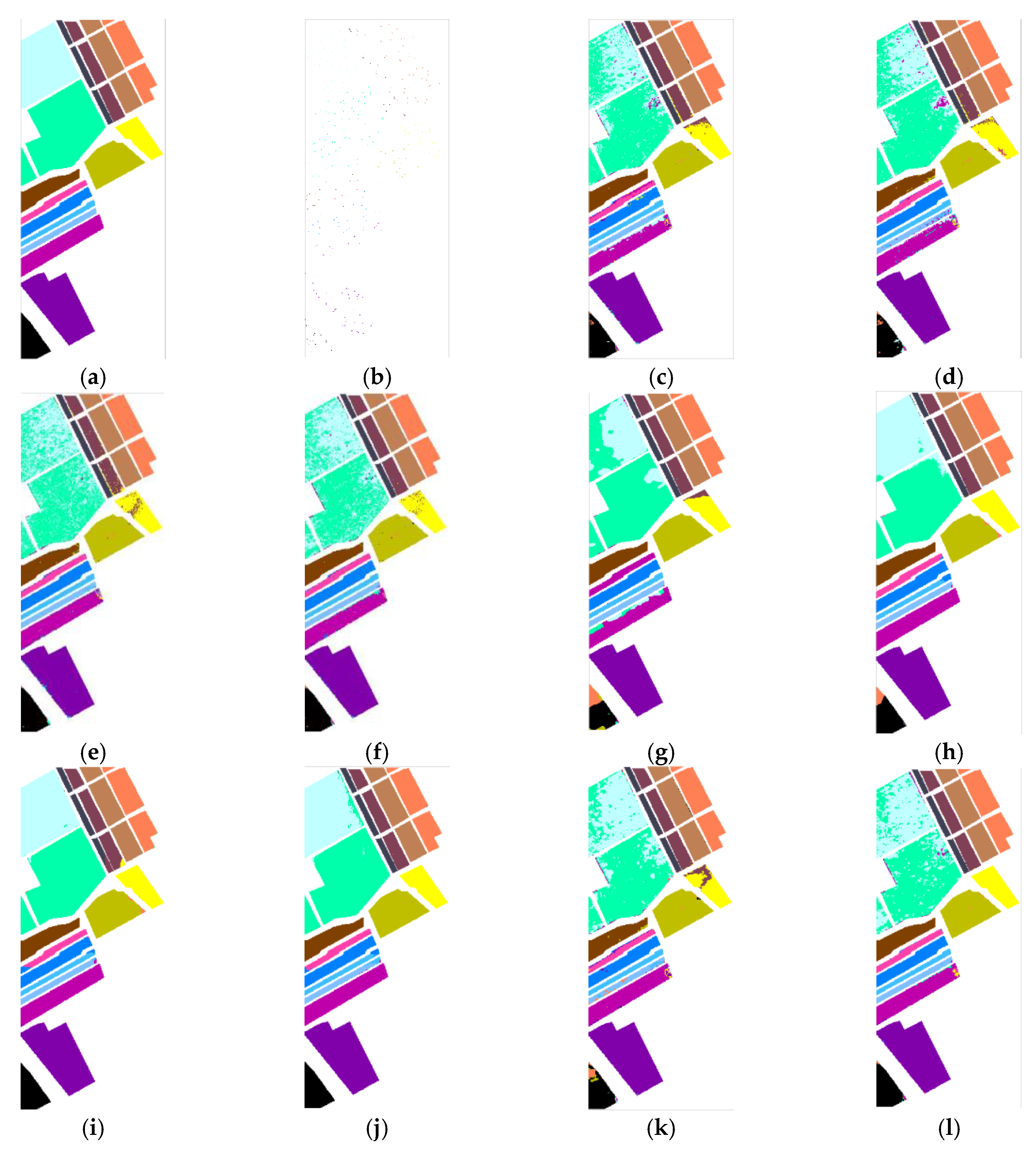
Likewise, the distribution based on Kennedy Space Center dataset is shown in Figure 10a: all 16 classes were selected, of which 4% (about 208) samples were employed as the training set, and the remaining 96% were used as the test set. Table 5 and Table 6 lists the classification accuracies of the Salinas Valley dataset for different methods. The classification effect is shown in Figure 10.
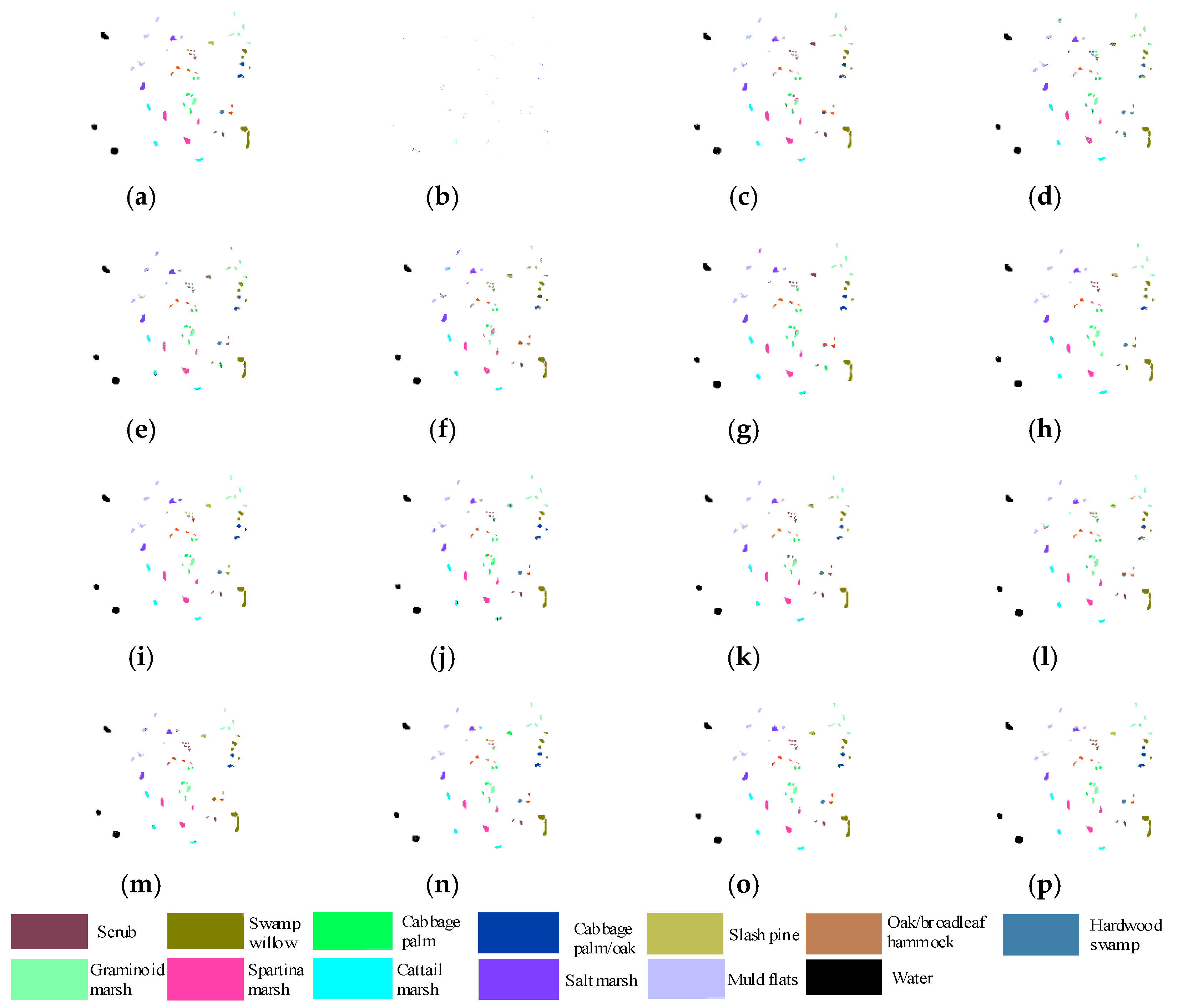
The classification results for Kennedy Space Center are shown in Figure 10, while Table 5 and Table 6 indicates the accuracies of OA, AA and Kappa for each class of the various methods, with the best accuracy of CFDTRF-LDM as OA = 97.33%, AA = 96.13% and Kappa = 97.03%. Furthermore, six classes for CFDTRF-LDM owned accuracies more than 99%. This experiment shows that the classification performance was enhanced compared to other classification methods.
Also, the OA values of CFDTRF-LDM were correspondingly larger than that of SVM, PCA-SVM, LDM, PCA-LDM, EPF, IFRF, LDM-FL, CF-SVM, CF-LDM, GDF-LDM, DTRF-SVM and DTRF-LDM by 14.89%, 17.85%, 12.23%, 16.69%, 8.31%, 10.17%, 3.21%, 7.16%, 7.27%, 6.32%, 4.72% and 2.10%. The hyperspectral classification completely verified the effectiveness of CFDTRF-LDM.
3.5.5. Analysis
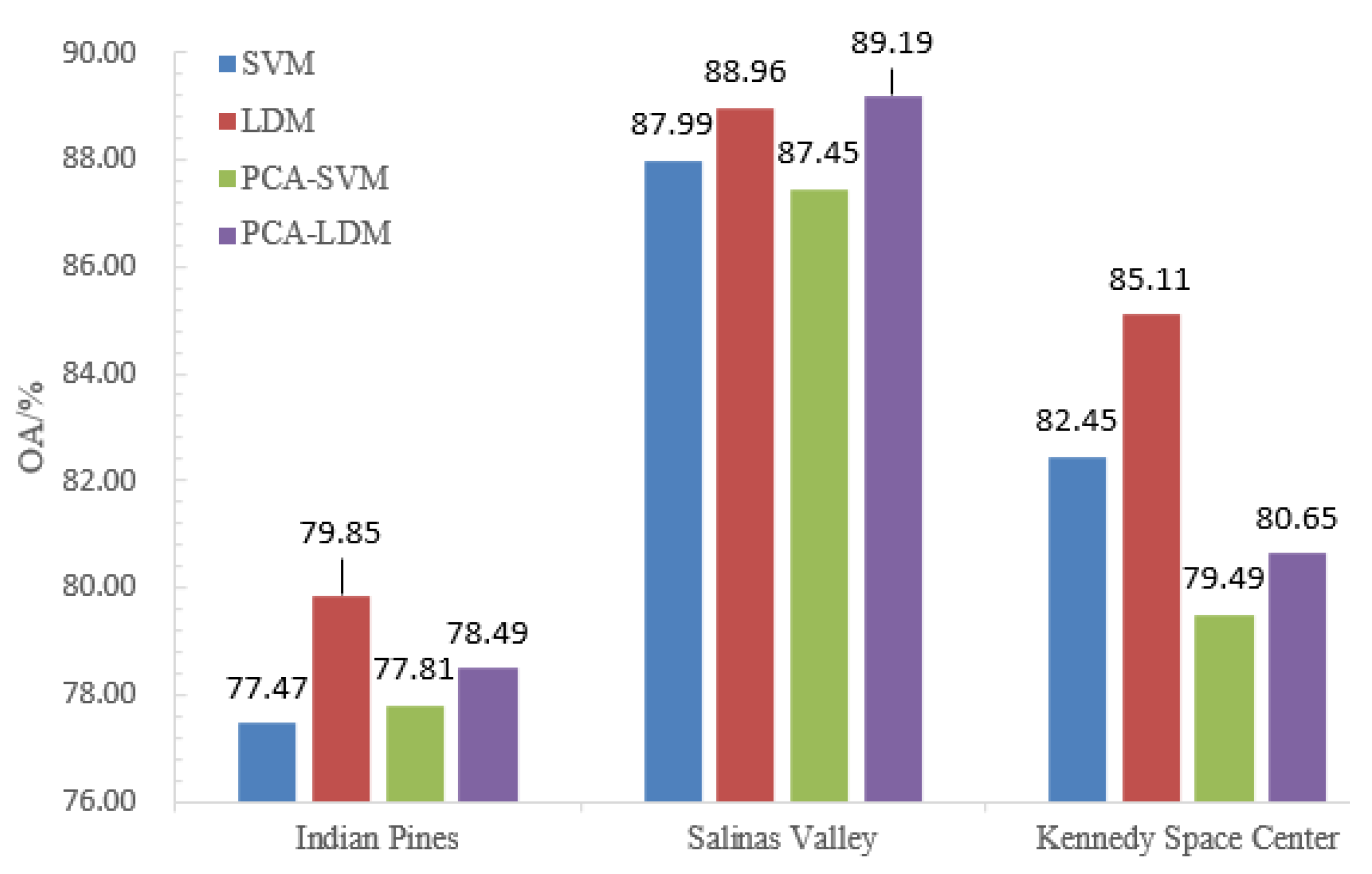
First, as the classification results are shown in Figure 11. The OA values of LDM and PCA-LDM for Indian Pines were 79.85% and 78.49%, correspondingly, which were 2.38% and 0.68% greater than that of SVM and PCA-SVM. Likewise, the OA values of LDM and PCA-LDM for Salinas Valley were 88.96% and 89.19%, respectively which were 0.98% and 1.74% higher than that of SVM and PCA-SVM. Furthermore, the OA values of LDM and PCA-LDM for the Kennedy Space Center were 85.11% and 80.65%, severally, which were 2.66% and 1.16% grander than that of SVM and PCA-SVM. It can be included that LDM superior to SVM with features that maximize margin means and minimize margin variances.
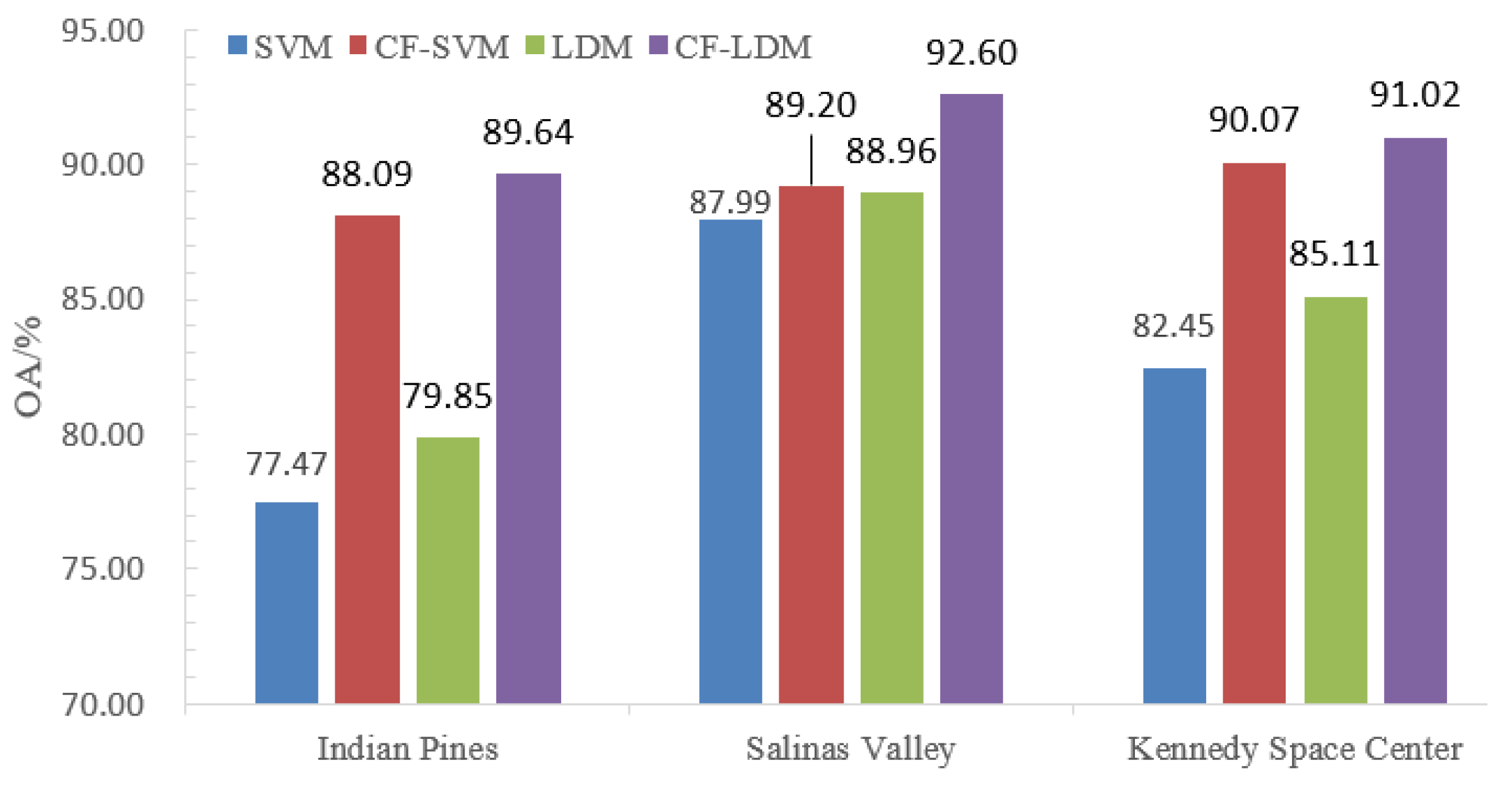
Second, as shown in Figure 12, the CF-SVM and CF-LDM OA values of Indian Pines were 10.62% and 9.79% higher than that of SVM and LDM, respectively, and the OA values of CF-SVM and CF-LDM in Salinas Valley were 1.21% and 1.60% higher than that of SVM and LDM. In addition, The OA values of CF-SVM and CF-LDM in Kennedy Space Center were 7.62% and 5.91% higher than that of SVM and LDM. This finding indicates that the spatial texture information extracted by CF was effective for enhancing the classification performance of SVM and LDM.
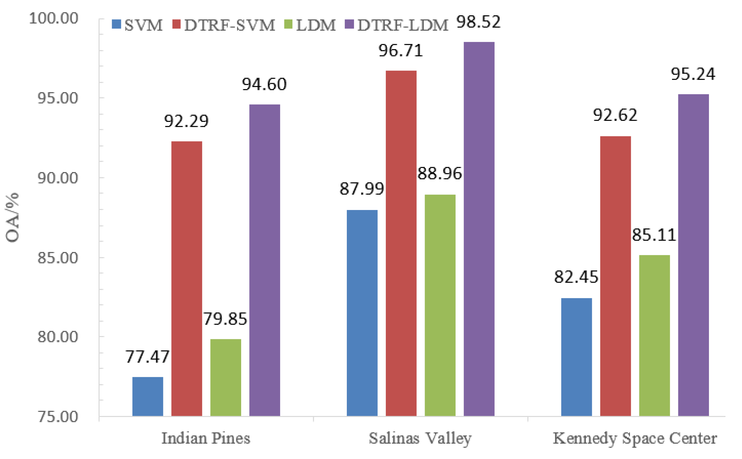
Third, from Figure 13, the OA values of DTRF-SVM and DTRF -LDM in Indian Pines were 14.82% and 14.75%, separately larger than of the OA values of SVM and LDM. Correspondingly, the OA values of DTRF-SVM and DTRF-LDM in Salinas Valley were 8.72% and 9.56% huger than the SVM and LDM OA values. Similarly, the OA values of DTRF-SVM and DTRF-LDM in Kennedy Space Center were 10.17% and 10.13%, respectively, higher than the SVM and LDM OA values. Thus, for improving the hyperspectral classification in this work, the spatial correlation information extracted by DTRF was efficient.
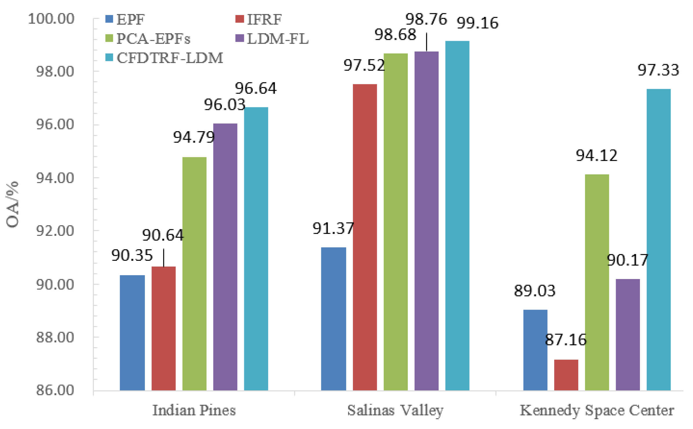
Fourth, in Figure 14, the OA values of CFDTRF-LDM in Indian Pines, Salinas Valley and Kennedy Space Center were 96.64%, 99.16% and 97.33%, respectively. It can be found that all those OA values were larger than that of EPF, IFRF, PCA-EPFs and LDM-FL. Therefore, the spatial texture information and spatial correlation information obtained by CF and DTRF in this work can improve the performance of LDM than that of the edge-preserving filter and recursive filter methods, and the LDM-based methods.
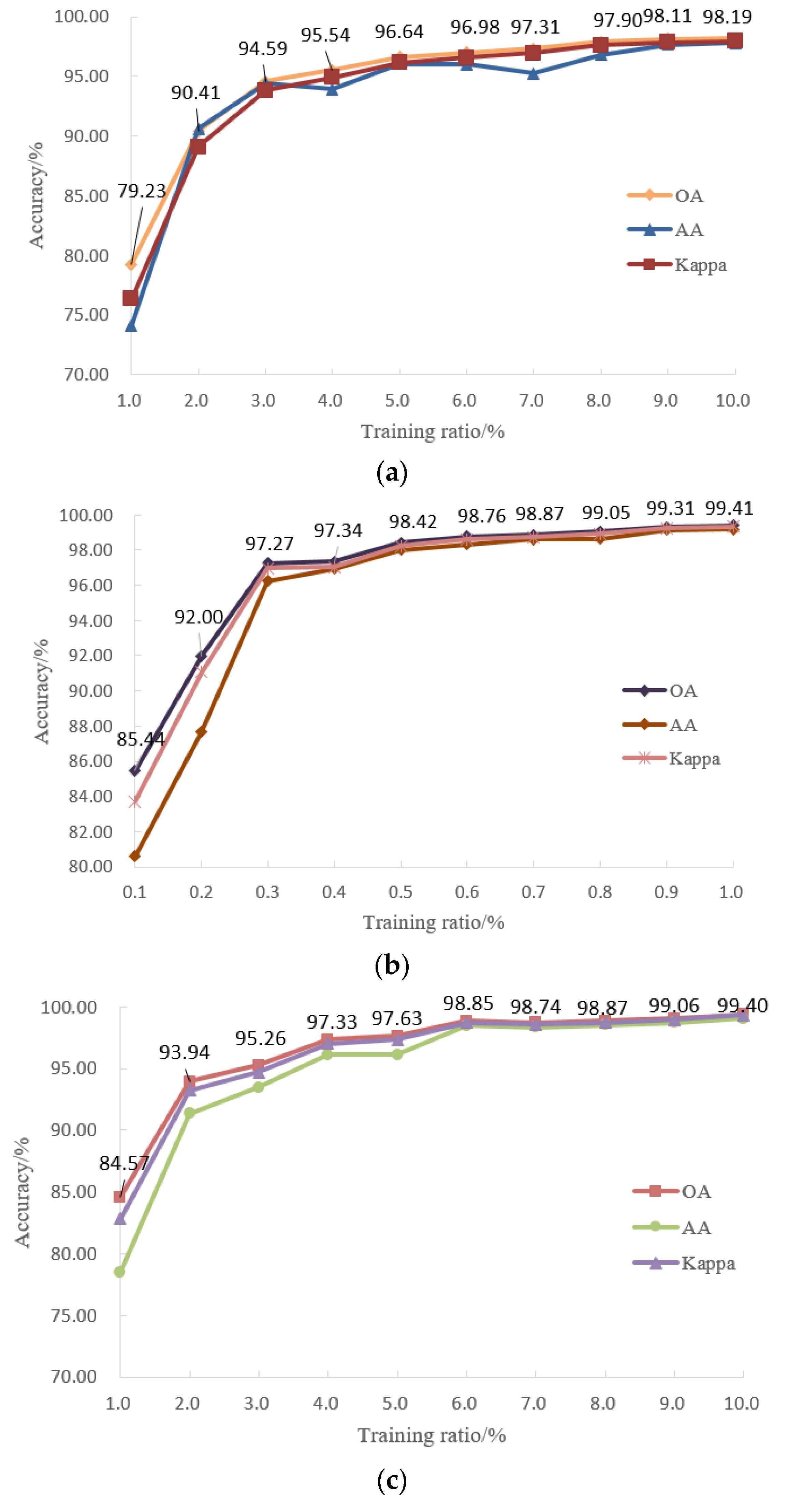
To prove the effect of the training ratio on the classification, the classification of the two datasets has been used to test the different values, as shown in Figure 15. As can be seen from the figure, if the training sample was 2% of the Indian Pines dataset, the OA value of the proposed method can reach 90.41%. In addition, when the ratio increased 7%, the OA value can exceed 97%. Also, if the training sample ratio of the Salinas Valley dataset was set to 0.2%, the OA value can reach 90%, and when the ratio increased to 0.8%, it can achieve to 99%. Also, when the training ratio were 2% and 9%, the OA value of the Kennedy Space Center can reach 93% and 99%, respectively. Thus, the proposed CFDTRF-LDM can obtain satisfied classification with a small amount of training set and provided stability of the different training ratios with optimal classification performance.
4. Conclusions
In this paper, based on the combination of two spatial information and LDM classification, namely CFDTRF-LDM, a hyperspectral image classification method was proposed. The spatial texture features and spatial correlation features were correspondingly extracted by CF and DTRF, which were linearly fused for the LDM classification. To verify the superior performance of CFDTRF-LDM, three hyperspectral image datasets were tested and found that the proposed method was superior to other methods. The advantage of the proposed method CFDTRF-LDM was that the spatial texture information and spatial correlation information extracted by CF and DTRF were appropriately fused to effectively classify with LDM, and obtain huge classification performance for HSI. Furthermore, the proposed method can obtain satisfied classification with a small amount of training set and supply stability of the various training ratios with optimal classification performance. For future work, more efficient spatial information should be explored for SVM or LDM classification.
Author Contributions
J.L. conceived and designed the methodology and experiments, and he also wrote, reviewed and edited the manuscript; L.W. analysis and interpretation of the results, aided the experimental verification and revised the manuscript.
Funding
This work was supported by the National Natural Science Foundation of China (Grant No 61275010 and 61675051), Natural Science Foundation of Guangdong (Grant No 2018A030313195), Major research project of Guangdong (Grant No 2017GKTSCX021), Science and Technology Project of Guangzhou (Grant No 201804010262), Science and Technology Project of Guangdong (Grant No 2017ZC0358).
Conflicts of Interest
The authors declare no conflict of interest.
References
- Guo, Y.; Cao, H.; Bai, J.; Bai, Y. High Efficient Deep Feature Extraction and Classification of Spectral-Spatial Hyperspectral Image Using Cross Domain Convolutional Neural Networks. IEEE J. Sel. Top. Appl. Earth Obs. Remote Sens. 2019, 12, 345–356. [Google Scholar] [CrossRef]
- Yu, C.; Wang, Y.; Song, M.; Chang, C. Class Signature-Constrained Background-Suppressed Approach to Band Selection for Classification of Hyperspectral Images. IEEE Trans. Geosci. Remote Sens. 2019, 57, 14–31. [Google Scholar] [CrossRef]
- Wang, X.; Zhong, Y.; Zhang, L.; Xu, Y. Spatial Group Sparsity Regularized Nonnegative Matrix Factorization for Hyperspectral Unmixing. IEEE Trans. Geosci. Remote Sens. 2017, 51, 6287–6304. [Google Scholar]
- Xu, X.; Li, J.; Wu, C.; Plaza, A. Regional clustering-based spatial preprocessing for hyperspectral unmixing. Remote Sens. Environ. 2018, 204, 333–346. [Google Scholar] [CrossRef]
- Chinsu, L.; Shih-Yu, C.; Chia-Chun, C.; Chia-Huei, T. Detecting newly grown tree leaves from unmanned-aerial-vehicle images using hyperspectral target detection techniques. Isprs J. Photogramm. Remote Sens. 2018, 142, 174–189. [Google Scholar]
- Dong, Y.; Du, B.; Zhang, L.; Hu, X. Hyperspectral Target Detection via Adaptive Information—Theoretic Metric Learning with Local Constraints. Remote Sens. 2018, 10, 1415. [Google Scholar]
- Shivers, S.W.; Roberts, D.A.; McFadden, J.P. Using paired thermal and hyperspectral aerial imagery to quantify land surface temperature variability and assess crop stress within California orchards. Remote Sens. Environ. 2019, 222, 215–231. [Google Scholar] [CrossRef]
- Awad, M. Sea water chlorophyll-a estimation using hyperspectral images and supervised artificial neural network. Ecol. Inform. 2014, 24, 60–68. [Google Scholar] [CrossRef]
- Ramirez, F.J.R.; Navarro-Cerrillo, R.M.; Varo-Martínez, M.Á.; Quero, J.L.; Doerr, S.; Hernández-Clemente, R. Determination of forest fuels characteristics in mortality-affected Pinus forests using integrated hyperspectral and ALS data. Int. J. Appl. Earth Obs. Geoinf. 2018, 68, 157–167. [Google Scholar] [CrossRef]
- Laakso, K.; Turner, D.J.; Rivard, B.; Sánchez-Azofeifa, A. The long-wave infrared (8–12 μm) spectral features of selected rare earth element—Bearing carbonate, phosphate and silicate minerals. Int. J. Appl. Earth Obs. Geoinf. 2019, 76, 77–83. [Google Scholar] [CrossRef]
- Awad, M.M. Forest mapping: A comparison between hyperspectral and multispectral images and technologies. J. For. Res. 2018, 29, 1395–1405. [Google Scholar] [CrossRef]
- Li, C.; Ma, Y.; Mei, X.; Ma, J. Hyperspectral image classification with robust sparse representation. IEEE Geosci. Remote Sens. Lett. 2016, 13, 641–645. [Google Scholar] [CrossRef]
- Golipour, M.; Ghassemian, H.; Mirzapour, F. Integrating hierarchical segmentation maps with MRF prior for classification of hyperspectral images in a Bayesian framework. IEEE Trans. Geosci. Remote Sens. 2016, 54, 805–816. [Google Scholar] [CrossRef]
- Guo, Y.; Cao, H.; Han, S.; Sun, Y.; Bai, Y. Spectral-Spatial Hyperspectral Image Classification with K-Nearest Neighbor and Guided Filter. IEEE Access 2018, 6, 18582–18591. [Google Scholar] [CrossRef]
- Richards, J.A.; Jia, X. Using Suitable Neighbors to Augment the Training Set in Hyperspectral Maximum Likelihood Classification. IEEE Geosci. Remote Sens. Lett. 2008, 5, 774–777. [Google Scholar] [CrossRef]
- Cao, F.; Yang, Z.; Ren, J.; Ling, W.K.; Zhao, H.; Marshall, S. Extreme sparse multinomial logistic regression: A fast and robust framework for hyperspectral image classification. Remote Sens. 2017, 9, 1255. [Google Scholar] [CrossRef]
- Aptoula, E.; Ozdemir, M.C.; Yanikoglu, B. Deep learning with attribute profiles for hyperspectral image classification. IEEE Geosci. Remote Sens. Lett. 2016, 13, 1970–1974. [Google Scholar] [CrossRef]
- Melgani, F.; Bruzzone, L. Classification of hyperspectral remote sensing images with support vector machines. IEEE Trans. Geosci. Remote Sens. 2004, 42, 1778–1790. [Google Scholar] [CrossRef]
- Zhang, T.; Zhou, Z.H. Large margin distribution machine. In Proceedings of the 20th ACM SIGKDD international conference on Knowledge discovery and data mining, New York, NY, USA, 24–27 August 2014; pp. 313–322. [Google Scholar]
- Zhan, K.; Wang, H.; Huang, H.; Xie, Y. Large margin distribution machine for hyperspectral image classification. J. Electron. Imaging 2016, 25, 063024. [Google Scholar] [CrossRef]
- Tarabalka, Y.; Chanussot, J.; Jón Atli, B. Segmentation and Classification of Hyperspectral Images Using Minimum Spanning Forest Grown from Automatically Selected Markers. IEEE Trans. Syst. Manand Cybern. Part B (Cybern.) 2010, 40, 1267–1279. [Google Scholar] [CrossRef]
- Ghamisi, P.; Couceiro, M.S.; Fauvel, M.; Benediktsson, J.A. Integration of Segmentation Techniques for Classification of Hyperspectral Images. IEEE Geosci. Remote Sens. Lett. 2014, 11, 342–346. [Google Scholar] [CrossRef]
- Huang, X.; Guan, X.; Benediktsson, J.A.; Zhang, L.; Plaza, A.; Mura, M.D. Multiple Morphological Profiles from Multicomponent-Base Images for Hyperspectral Image Classification. IEEE J. Sel. Top. Appl. Earth Obs. Remote Sens. 2014, 7, 4653–4669. [Google Scholar] [CrossRef]
- Xue, Z.; Li, J.; Cheng, L.; Du, P. Spectral–Spatial Classification of Hyperspectral Data via Morphological Component Analysis-Based Image Separation. IEEE Trans. Geosci. Remote Sens. 2015, 53, 70–84. [Google Scholar]
- Gastal, E.S.L.; Oliveira, M.M. Domain transform for edge-aware image and video processing. In Proceedings of the ACM Transactions on Graphics (ToG), Vancouver, BC, Canada, 7–11 August 2011; Volume 30, p. 69. [Google Scholar]
- Liao, J.; Wang, L.; Hao, S. Hyperspectral image classification based on adaptive optimisation of morphological profile and spatial correlation information. Int. J. Remote Sens. 2018, 39, 9159–9180. [Google Scholar] [CrossRef]
- Zhang, Y.; Brady, M.; Smith, S. Segmentation of brain MR images through a hidden Markov random field model and the expectation-maximization algorithm. IEEE Trans. Med Imaging 2001, 20, 45–57. [Google Scholar] [CrossRef]
- Sun, L.; Wu, Z.; Liu, J.; Xiao, L.; Wei, Z. Supervised Spectral–Spatial Hyperspectral Image Classification with Weighted Markov Random Fields. IEEE Trans. Geosci. Remote Sens. 2014, 53, 1490–1503. [Google Scholar] [CrossRef]
- Zhang, X.; Gao, Z.; Jiao, L.; Zhou, H. Multifeature Hyperspectral Image Classification with Local and Nonlocal Spatial Information via Markov Random Field in Semantic Space. IEEE Trans. Geosci. Remote Sens. 2018, 56, 1409–1424. [Google Scholar] [CrossRef]
- He, K.; Sun, J.; Tang, X. Guided image filtering. IEEE Trans. Pattern Anal. Mach. Intell. 2013, 35, 1397–1409. [Google Scholar] [CrossRef] [PubMed]
- Tomasi, C.; Manduchi, R. Bilateral filtering for gray and color images. In Proceedings of the IEEE Sixth International Conference on Computer Vision, Bombay, India, 4–7 January 1998; pp. 839–846. [Google Scholar]
- Jones, J.P.; Palmer, L.A. An evaluation of the two-dimensional Gabor filter model of simple receptive fields in cat striate cortex. J. Neurophysiol. 1987, 58, 1233–1258. [Google Scholar] [CrossRef]
- Wang, Z.; Hu, H.; Zhang, L.; Xue, J.H. Discriminatively guided filtering (DGF) for hyperspectral image classification. Neurocomputing 2018, 275, 1981–1987. [Google Scholar] [CrossRef]
- Guo, Y.; Han, S.; Li, Y.; Zhang, C.; Bai, Y. K-Nearest Neighbor combined with guided filter for hyperspectral image classification. Procedia Comput. Sci. 2018, 129, 159–165. [Google Scholar] [CrossRef]
- Wang, Y.; Song, H.; Zhang, Y. Spectral-Spatial Classification of Hyperspectral Images Using Joint Bilateral Filter and Graph Cut Based Model. Remote Sens. 2016, 8, 748. [Google Scholar] [CrossRef]
- Sahadevan, A.S.; Routray, A.; Das, B.S.; Ahmad, S. Hyperspectral image preprocessing with bilateral filter for improving the classification accuracy of support vector machines. J. Appl. Remote Sens. 2016, 10, 025004. [Google Scholar] [CrossRef]
- Qiao, T.; Yang, Z.; Ren, J.; Yuen, P.; Zhao, H.; Sun, G.; Marshall, S.; Benediktsson, J.A. Joint bilateral filtering and spectral similarity-based sparse representation: A generic framework for effective feature extraction and data classification in hyperspectral imaging. Pattern Recognit. 2018, 77, 316–328. [Google Scholar] [CrossRef]
- Moore, B.C. Principal component analysis in linear systems: Controllability, observability, and model reduction. IEEE Trans. Autom. Control 2003, 26, 17–32. [Google Scholar] [CrossRef]
- Kang, X.; Li, S.; Benediktsson, J.A. Spectral-spatial hyperspectral image classification with edge-preserving filtering. IEEE Trans. Geosci. Remote Sens. 2014, 52, 2666–2677. [Google Scholar] [CrossRef]
- Kang, X.; Xiang, X.; Li, S.; Benediktsson, J.A. PCA-based edge-preserving features for hyperspectral image classification. IEEE Trans. Geosci. Remote Sens. 2017, 55, 7140–7151. [Google Scholar] [CrossRef]
- Kang, X.; Li, S.; Benediktsson, J.A. Feature extraction of hyperspectral images with image fusion and recursive filtering. IEEE Trans. Geosci. Remote Sens. 2014, 52, 3742–3752. [Google Scholar] [CrossRef]
- Jia, S.; Wu, K.; Zhu, J.; Jia, X. Spectral-Spatial Gabor Surface Feature Fusion Approach for Hyperspectral Imagery Classification. IEEE Trans. Geosci. Remote Sens. 2019, 57, 1142–1154. [Google Scholar] [CrossRef]
- Li, H.C.; Zhou, H.L.; Pan, L.; Du, Q. Gabor feature-based composite kernel method for hyperspectral image classification. Electron. Lett. 2018, 54, 628–630. [Google Scholar] [CrossRef]
- Chen, Y.; Zhu, L.; Ghamisi, P.; Jia, S.; Li, G.; Tang, L. Hyperspectral images classification with Gabor filtering and convolutional neural network. IEEE Geosci. Remote Sens. Lett. 2017, 14, 2355–2359. [Google Scholar] [CrossRef]
- Tu, B.; Zhang, X.; Wang, J.; Zhang, G.; Ou, X. Spectral-Spatial Hyperspectral Image Classification via Non-local Means Filtering Feature Extraction. Sens. Imaging 2018, 19, 11. [Google Scholar] [CrossRef]
- Gong, Y.; Sbalzarini, I.F. Curvature filters efficiently reduce certain variational energies. IEEE Trans. Image Process. 2017, 26, 1786–1798. [Google Scholar] [CrossRef]
- Zhang, H.; Jin, X.; Wu, Q.; Jonathan, W.Q.M.; He, Z.; Wang, Y. Automatic visual detection method of railway surface defects based on curvature filtering and improved GMM. Chin. J. Sci. Instrum. 2018, 39, 181–194. [Google Scholar]
- Gao, W.; Zhou, Z.H. On the doubt about margin explanation of boosting. Artif. Intell. 2013, 203, 1–18. [Google Scholar] [CrossRef]
- Moran, P.A.P. The interpretation of statistical maps. J. R. Stat. Soc. Ser. B (Methodol.) 1948, 10, 243–251. [Google Scholar] [CrossRef]
- Moran, P.A.P. Notes on continuous stochastic phenomena. Biometrika 1950, 37, 17–23. [Google Scholar] [CrossRef] [PubMed]
- Hao, S.; Wang, W.; Ye, Y.; Li, Y.; Bruzzone, L. A deep network architecture for super-resolution-aided hyperspectral image classification with classwise loss. IEEE Trans. Geosci. Remote Sens. 2018, 56, 4650–4663. [Google Scholar] [CrossRef]
- Cheng, G.; Li, Z.; Han, J.; Yao, X.; Guo, L. Exploring Hierarchical Convolutional Features for Hyperspectral Image Classification. IEEE Trans. Geosci. Remote Sens. 2018, 56, 6712–6722. [Google Scholar] [CrossRef]
Figure 1.
The evolution process of energy functional.

Figure 2.
Disjoint domain decomposition.

Figure 3.
All possible triangles in the neighborhood (a) down; (b) down and left (P); (c) mix.

Figure 4.
Eight types of the triangular tangent planes through (a) two of the common edges from the four tangent plane (R); (b) two of the common edges from the four tangent plane (P); (c) four of the tangent planes through mixed neighbors.
Figure 4.
Eight types of the triangular tangent planes through (a) two of the common edges from the four tangent plane (R); (b) two of the common edges from the four tangent plane (P); (c) four of the tangent planes through mixed neighbors.

Figure 5.
Flow of the proposed curvature filter domain transform recursive filter (CFDTRF-LDM).

Figure 6.
Curvature filter (CF) and domain transform recursive filter (DTRF) comparison for Indian Pines; (a) the 10th band of spectrum; (b) the 60th band of spectrum; (c) the 130th band of spectrum; (d) the 180th band of spectrum; (e) the 10th band filtering of CF; (f) the 60th band filtering of CF; (g) the 130th band filtering of CF; (h) the 180th band filtering of CF; (i) the 10th band filtering of DTRF; (j) the 60th band filtering of DTRF; (k) the 130th band filtering of DTRF; (h) the 180th band filtering of DTRF.


Figure 7.
Average of Moran’s I for hyperspectral images (HSI) (a) Indian Pines (b) Salinas Valley (c) Kennedy Space Center.
Figure 7.
Average of Moran’s I for hyperspectral images (HSI) (a) Indian Pines (b) Salinas Valley (c) Kennedy Space Center.

Figure 8.
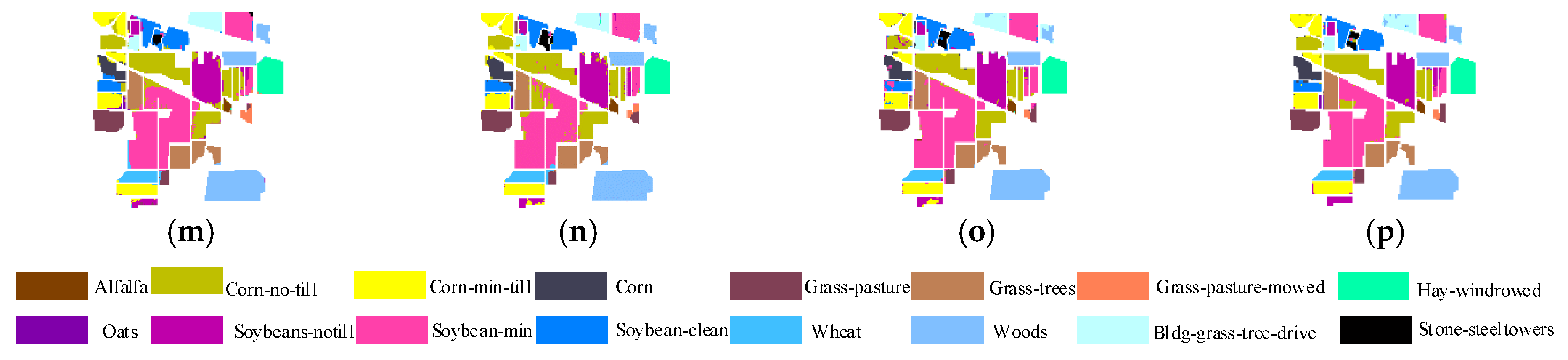
Classification maps of different methods on the Indian Pines dataset (a) ground; (b) training; (c) SVM, overall accuracy (OA) = 77.47%; (d) principal component analysis (PCA)-SVM, OA = 77.81% (e) large margin distribution machine (LDM), OA = 79.85%; (f) PCA-LDM, OA = 78.49%; (g) edge-preserving filter (EPF), OA = 90.35%; (h) image fusion with multiple subsets of adjacent bands and recursive filter (IFRF), OA = 90.64%; (i) PCA-EPFs, OA = 91.62%; (j) LDM-FL, OA = 93.31%; (k) CF-SVM, OA = 88.09%; (l) CF-LDM, OA = 88.54%; (m) DTRF-SVM, OA = 92.29%; (n) DTRF-LDM, OA = 94.60%; (o) CFDTRFF-SVM, OA = 94.13%; (p) CFDTRF-LDM, OA = 96.64%.
Figure 8.
Classification maps of different methods on the Indian Pines dataset (a) ground; (b) training; (c) SVM, overall accuracy (OA) = 77.47%; (d) principal component analysis (PCA)-SVM, OA = 77.81% (e) large margin distribution machine (LDM), OA = 79.85%; (f) PCA-LDM, OA = 78.49%; (g) edge-preserving filter (EPF), OA = 90.35%; (h) image fusion with multiple subsets of adjacent bands and recursive filter (IFRF), OA = 90.64%; (i) PCA-EPFs, OA = 91.62%; (j) LDM-FL, OA = 93.31%; (k) CF-SVM, OA = 88.09%; (l) CF-LDM, OA = 88.54%; (m) DTRF-SVM, OA = 92.29%; (n) DTRF-LDM, OA = 94.60%; (o) CFDTRFF-SVM, OA = 94.13%; (p) CFDTRF-LDM, OA = 96.64%.


Figure 9.
Classification maps of different methods on the Salinas Valley dataset (a) ground; (b) training; (c) SVM, OA = 87.99%; (d) PCA-SVM, OA = 87.45%; (e) LDM, OA = 88.96%; (f) PCA-LDM, OA = 89.19%; (g) EPF, OA = 91.37%; (h) IFRF, OA = 97.52%; (i) PCA-EPFs, OA = 98.68%; (j) LDM-FL, OA = 98.76%; (k) CF-SVM, OA = 89.20%; (l) CF-LDM, OA = 90.56%; (m) DTRF-SVM, OA = 96.71%; (n) DTRF-LDM, OA = 98.52%; (o) CFDTRFF-SVM, OA = 97.93%; (p) CFDTRF-LDM, OA = 99.16%.


Figure 10.
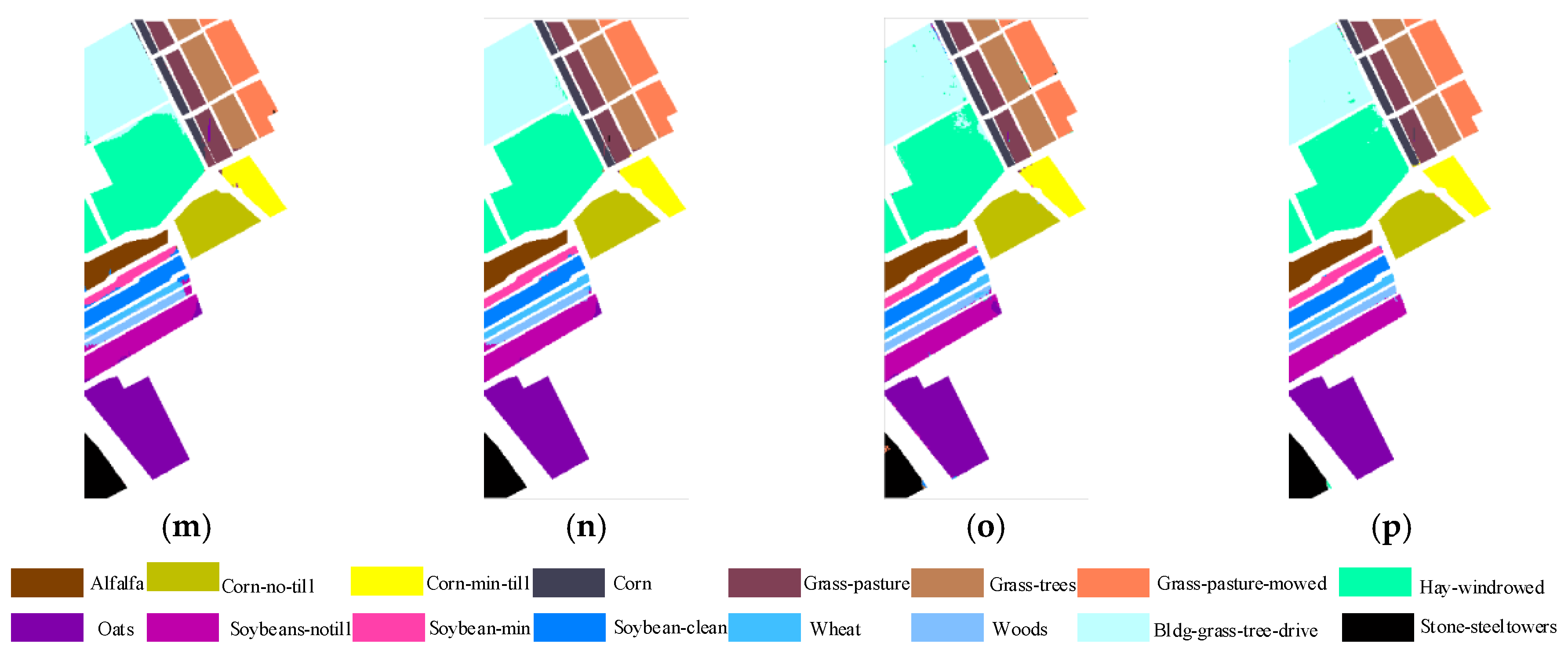
Classification maps of different methods on the Salinas Valley dataset (a) Ground; (b) Training; (c) SVM, OA = 82.45%; (d) PCA-SVM, OA = 79.49%; (e) LDM, OA = 85.11%; (f) PCA-LDM, OA = 80.65%; (g) EPF, OA = 89.03%; (h) IFRF, OA = 86.21%; (i) PCA-EPFs, OA = 94.12%; (j) LDM-FL, OA = 90.17%; (k) CF-SVM, OA = 90.07%; (l) CF-LDM, OA = 91.02%; (m) DTRF-SVM, OA = 92.62%; (n) DTRF-LDM, OA = 95.24%; (o) CFDTRFF-SVM, OA = 95.89%; (p) CFDTRF-LDM, OA = 97.33%.
Figure 10.
Classification maps of different methods on the Salinas Valley dataset (a) Ground; (b) Training; (c) SVM, OA = 82.45%; (d) PCA-SVM, OA = 79.49%; (e) LDM, OA = 85.11%; (f) PCA-LDM, OA = 80.65%; (g) EPF, OA = 89.03%; (h) IFRF, OA = 86.21%; (i) PCA-EPFs, OA = 94.12%; (j) LDM-FL, OA = 90.17%; (k) CF-SVM, OA = 90.07%; (l) CF-LDM, OA = 91.02%; (m) DTRF-SVM, OA = 92.62%; (n) DTRF-LDM, OA = 95.24%; (o) CFDTRFF-SVM, OA = 95.89%; (p) CFDTRF-LDM, OA = 97.33%.

Figure 11.
Comparison of SVM, LDM, PCA-SVM and PCA-LDM on three datasets.

Figure 12.
Comparison of SVM, CF-SVM, LDM and CF-LDM on three datasets.

Figure 13.
Comparison of SVM, DTRF-SVM, LDM and DTRF-LDM on three datasets.

Figure 14.
Comparison of EPF, PCA-EPFs, IFRF, LDM-FL and CFDTRF-LDM on three datasets.

Figure 15.
Effect of different training ratios on classification performance (a) Indian Pines (b) Salinas Valley (c) Kennedy Space Center.
Figure 15.
Effect of different training ratios on classification performance (a) Indian Pines (b) Salinas Valley (c) Kennedy Space Center.


Table 1.
Comparison of classification accuracies (in percent) provided by seven methods for Indian Pines (part A).
Table 1.
Comparison of classification accuracies (in percent) provided by seven methods for Indian Pines (part A).
| Ground | Sum | Train | SVM | PCA-SVM | LDM | PCA-LDM | EPF | IFRF | PCA-EPFs |
|---|---|---|---|---|---|---|---|---|---|
| Alfalfa | 54 | 11 | 45.59 | 73.20 | 90.08 | 83.42 | 55.88 | 89.51 | 83.28 |
| Corn-no-till | 1434 | 72 | 64.06 | 67.16 | 72.90 | 74.16 | 84.55 | 89.87 | 86.18 |
| Corn-min-till | 834 | 42 | 72.28 | 71.24 | 67.41 | 57.38 | 88.49 | 78.09 | 91.12 |
| Corn | 234 | 12 | 15.73 | 34.51 | 56.38 | 60.08 | 19.11 | 69.25 | 78.80 |
| Grass-pasture | 497 | 25 | 87.22 | 84.36 | 88.90 | 91.85 | 91.56 | 92.72 | 91.49 |
| Grass-trees | 747 | 37 | 94.11 | 95.83 | 94.98 | 94.35 | 99.89 | 97.97 | 93.53 |
| Grass-pasture-mowed | 26 | 5 | 45.46 | 73.57 | 83.57 | 69.11 | 43.86 | 64.18 | 60.59 |
| Hay-windrowed | 489 | 24 | 98.26 | 96.96 | 96.46 | 94.62 | 100.00 | 99.51 | 99.83 |
| Oats | 20 | 4 | 29.46 | 26.68 | 73.53 | 87.85 | 18.30 | 41.29 | 42.32 |
| Soybeans-no-till | 968 | 48 | 65.89 | 61.67 | 67.49 | 72.83 | 86.69 | 84.51 | 87.86 |
| Soybeans-min-till | 2468 | 123 | 82.38 | 82.87 | 79.34 | 73.30 | 97.83 | 94.58 | 96.35 |
| Soybeans-clean-till | 614 | 31 | 76.40 | 76.03 | 80.35 | 73.29 | 95.47 | 89.31 | 88.21 |
| Wheat | 212 | 11 | 95.66 | 98.28 | 99.51 | 99.01 | 99.88 | 99.16 | 76.38 |
| Woods | 1294 | 65 | 95.64 | 97.25 | 92.65 | 91.81 | 99.57 | 98.55 | 98.36 |
| Bldg-grass-tree | 380 | 19 | 41.31 | 33.53 | 61.07 | 56.65 | 53.77 | 76.75 | 91.20 |
| Stone-steel-towers | 95 | 5 | 81.22 | 57.49 | 86.38 | 76.38 | 93.87 | 67.63 | 58.59 |
| OA/% | - | 77.47 | 77.81 | 79.85 | 78.49 | 90.35 | 90.64 | 91.62 | |
| AA/% | - | 68.17 | 70.66 | 80.69 | 78.51 | 76.80 | 83.31 | 82.76 | |
| Kappa/% | - | 74.12 | 74.52 | 77.03 | 77.36 | 88.92 | 89.30 | 90.43 |
Table 2.
Comparison of classification accuracies (in percent) provided by seven methods for Indian Pines (part B).
Table 2.
Comparison of classification accuracies (in percent) provided by seven methods for Indian Pines (part B).
| Ground | Sum | Train | LDM-FL | CF-SVM | CF-LDM | DTRF-SVM | DTRF-LDM | CFDTRFF-SVM | CFDTRF-LDM |
|---|---|---|---|---|---|---|---|---|---|
| Alfalfa | 54 | 11 | 93.13 | 86.69 | 89.41 | 92.38 | 98.73 | 76.32 | 93.62 |
| Corn-no-till | 1434 | 72 | 92.17 | 84.60 | 86.26 | 87.98 | 91.07 | 94.74 | 96.85 |
| Corn-min-till | 834 | 42 | 89.89 | 83.40 | 81.41 | 92.51 | 92.21 | 92.29 | 94.71 |
| Corn | 234 | 12 | 77.60 | 69.97 | 73.33 | 78.79 | 94.72 | 73.56 | 88.17 |
| Grass-pasture | 497 | 25 | 93.43 | 94.71 | 94.67 | 89.58 | 96.36 | 92.68 | 92.29 |
| Grass-trees | 747 | 37 | 96.56 | 97.39 | 98.51 | 94.76 | 97.01 | 97.32 | 99.01 |
| Grass-pasture-mowed | 26 | 5 | 100.0 | 74.11 | 97.50 | 27.94 | 100.0 | 98.61 | 93.45 |
| Hay-windrowed | 489 | 24 | 100.00 | 98.65 | 98.80 | 99.78 | 100.00 | 99.40 | 99.78 |
| Oats | 20 | 4 | 93.74 | 52.35 | 98.33 | 5.88 | 93.20 | 70.31 | 100.00 |
| Soybeans-no-till | 968 | 48 | 91.57 | 78.69 | 85.60 | 86.39 | 92.45 | 87.69 | 95.21 |
| Soybeans-min-till | 2468 | 123 | 92.56 | 91.60 | 86.97 | 95.57 | 95.02 | 96.80 | 96.97 |
| Soybeans-clean-till | 614 | 31 | 91.17 | 87.21 | 86.19 | 89.96 | 90.69 | 91.53 | 92.06 |
| Wheat | 212 | 11 | 99.14 | 99.12 | 99.26 | 97.24 | 94.09 | 99.25 | 99.75 |
| Woods | 1294 | 65 | 98.98 | 98.34 | 96.48 | 98.74 | 99.67 | 98.82 | 99.96 |
| Bldg-grass-tree | 380 | 19 | 90.20 | 48.87 | 68.97 | 92.66 | 93.68 | 91.12 | 99.16 |
| Stone-steel-towers | 95 | 5 | 92.09 | 84.00 | 88.38 | 67.51 | 81.45 | 70.04 | 95.67 |
| OA/% | - | 93.31 | 88.09 | 88.54 | 92.29 | 94.60 | 94.13 | 96.64 | |
| AA/% | - | 93.26 | 83.11 | 89.38 | 81.10 | 94.40 | 89.41 | 96.04 | |
| Kappa/% | - | 92.39 | 86.36 | 86.94 | 91.20 | 93.84 | 93.29 | 96.16 |
Table 3.
Comparison of classification accuracies (in percent) provided by seven methods for Salinas Valley (part A).
Table 3.
Comparison of classification accuracies (in percent) provided by seven methods for Salinas Valley (part A).
| Ground | Sum | Training | SVM | PCA-SVM | LDM | PCA-LDM | EPF | IFRF | PCA-EPFs |
|---|---|---|---|---|---|---|---|---|---|
| Broccoli-green-weeds-1 | 2009 | 16 | 96.68 | 98.91 | 99.06 | 99.32 | 99.84 | 99.93 | 99.86 |
| Broccoli green-weeds-2 | 3726 | 30 | 99.03 | 98.59 | 99.08 | 99.03 | 100.00 | 98.88 | 99.43 |
| Fallow | 1976 | 16 | 95.91 | 85.30 | 94.30 | 98.04 | 86.58 | 99.96 | 99.66 |
| Fallow-rough-plough | 1394 | 11 | 96.34 | 94.50 | 99.06 | 99.35 | 99.87 | 95.11 | 92.39 |
| Fallow-smooth | 2678 | 21 | 90.60 | 97.33 | 95.97 | 96.51 | 99.50 | 96.28 | 98.29 |
| Stubble | 3959 | 32 | 99.57 | 99.50 | 99.84 | 99.76 | 100.00 | 99.62 | 99.84 |
| Celery | 3579 | 29 | 99.35 | 99.34 | 99.61 | 99.46 | 100.00 | 99.16 | 99.18 |
| Grapes-untrained | 11271 | 90 | 89.94 | 86.19 | 78.05 | 76.14 | 95.01 | 96.04 | 98.45 |
| Soil-vineyard-develop | 6203 | 50 | 98.22 | 99.00 | 99.35 | 99.60 | 99.96 | 100.00 | 100.00 |
| Corn-senesced-green weeds | 3278 | 26 | 89.33 | 83.14 | 92.17 | 93.11 | 92.23 | 99.02 | 99.41 |
| Lettuce-romaine-4wk | 1068 | 9 | 70.95 | 66.80 | 92.34 | 91.60 | 97.76 | 90.80 | 88.48 |
| Lettuce-romaine-5wk | 1927 | 15 | 98.29 | 93.45 | 99.69 | 99.62 | 100.00 | 98.08 | 98.45 |
| Lettuce-romaine-6wk | 916 | 7 | 98.43 | 50.42 | 97.66 | 97.99 | 100.00 | 83.46 | 96.41 |
| Lettuce-romaine-7wk | 1070 | 9 | 88.09 | 94.49 | 94.12 | 95.50 | 99.60 | 95.31 | 96.89 |
| Vineyard-untrained | 7268 | 58 | 51.00 | 61.05 | 63.39 | 65.96 | 53.39 | 97.89 | 99.86 |
| Vineyard-vertical-trellis | 1807 | 14 | 81.60 | 86.77 | 96.47 | 97.13 | 91.75 | 93.45 | 95.86 |
| OA/% | - | 87.99 | 87.45 | 88.96 | 89.19 | 91.37 | 97.52 | 98.68 | |
| AA/% | - | 90.21 | 87.17 | 93.76 | 94.26 | 94.72 | 96.44 | 97.65 | |
| Kappa/% | - | 86.57 | 85.96 | 87.70 | 87.97 | 90.34 | 97.23 | 98.53 |
Table 4.
Comparison of classification accuracies (in percent) provided by seven methods for Salinas Valley (part B).
Table 4.
Comparison of classification accuracies (in percent) provided by seven methods for Salinas Valley (part B).
| Ground | Sum | Training | LDM-FL | CF-SVM | CF-LDM | DTRF-SVM | DTRF-LDM | CFDTRFF-SVM | CFDTRF-LDM |
|---|---|---|---|---|---|---|---|---|---|
| Broccoli-green-weeds-1 | 2009 | 16 | 99.99 | 99.91 | 99.95 | 99.96 | 100.00 | 100.00 | 100.00 |
| Broccoli green-weeds-2 | 3726 | 30 | 99.75 | 97.44 | 99.57 | 99.36 | 99.81 | 99.80 | 99.98 |
| Fallow | 1976 | 16 | 99.96 | 92.66 | 99.95 | 97.74 | 98.31 | 97.05 | 100.00 |
| Fallow-rough-plough | 1394 | 11 | 96.41 | 98.59 | 98.88 | 89.95 | 91.38 | 99.15 | 98.46 |
| Fallow-smooth | 2678 | 21 | 99.03 | 96.73 | 99.04 | 94.93 | 94.79 | 98.07 | 98.73 |
| Stubble | 3959 | 32 | 99.55 | 99.36 | 99.76 | 97.70 | 98.84 | 99.58 | 99.90 |
| Celery | 3579 | 29 | 99.85 | 99.57 | 99.76 | 99.87 | 99.83 | 99.73 | 99.72 |
| Grapes-untrained | 11271 | 90 | 98.50 | 87.98 | 83.92 | 97.82 | 99.24 | 97.54 | 99.18 |
| Soil-vineyard-develop | 6203 | 50 | 100.00 | 99.87 | 99.67 | 100.00 | 100.00 | 99.63 | 100.00 |
| Corn-senesced-green weeds | 3278 | 26 | 99.32 | 86.16 | 93.23 | 96.27 | 96.53 | 95.97 | 98.19 |
| Lettuce-romaine-4wk | 1068 | 9 | 91.08 | 56.40 | 94.38 | 64.07 | 94.06 | 96.65 | 96.84 |
| Lettuce-romaine-5wk | 1927 | 15 | 98.37 | 86.48 | 100.00 | 98.52 | 99.01 | 99.95 | 100.00 |
| Lettuce-romaine-6wk | 916 | 7 | 93.09 | 97.61 | 97.04 | 93.30 | 94.46 | 93.36 | 98.26 |
| Lettuce-romaine-7wk | 1070 | 9 | 95.06 | 89.91 | 97.41 | 74.42 | 94.66 | 91.38 | 93.20 |
| Vineyard-untrained | 7268 | 58 | 99.16 | 64.93 | 76.36 | 98.21 | 99.40 | 96.37 | 99.03 |
| Vineyard-vertical-trellis | 1807 | 14 | 96.24 | 88.78 | 97.80 | 95.21 | 99.43 | 95.69 | 97.82 |
| OA/% | - | 98.76 | 89.20 | 92.60 | 96.71 | 98.52 | 97.93 | 99.16 | |
| AA/% | - | 97.84 | 90.15 | 96.04 | 93.58 | 97.48 | 97.49 | 98.71 | |
| Kappa/% | - | 98.62 | 87.92 | 91.76 | 96.33 | 98.35 | 97.70 | 99.06 |
Table 5.
Comparison of classification accuracies (in percent) provided by seven methods for Kennedy Space Center (part A).
Table 5.
Comparison of classification accuracies (in percent) provided by seven methods for Kennedy Space Center (part A).
| Ground | Sum | Training | SVM | PCA-SVM | LDM | PCA-LDM | EPF | IFRF | PCA-EPFs |
|---|---|---|---|---|---|---|---|---|---|
| Scrub | 761 | 30 | 97.66 | 87.95 | 89.54 | 98.43 | 100.00 | 95.91 | 99.00 |
| Swamp willow | 243 | 10 | 85.42 | 70.41 | 84.78 | 68.98 | 81.12 | 35.46 | 59.96 |
| Cabbage palm hammock | 256 | 10 | 84.99 | 70.54 | 88.39 | 78.69 | 94.85 | 92.98 | 97.27 |
| Cabbage palm/oak | 252 | 10 | 49.68 | 46.28 | 55.33 | 44.40 | 80.40 | 57.85 | 97.32 |
| Slash pine | 161 | 6 | 8.28 | 38.67 | 52.71 | 26.32 | 12.83 | 63.77 | 64.70 |
| Oak/broadleaf hammock | 229 | 9 | 25.68 | 35.82 | 56.79 | 0.23 | 21.37 | 60.51 | 77.86 |
| Hardwood swamp | 105 | 4 | 38.89 | 57.99 | 66.96 | 41.09 | 48.51 | 77.87 | 81.76 |
| Graminoid marsh | 431 | 17 | 75.44 | 63.40 | 72.97 | 71.72 | 93.46 | 91.28 | 99.71 |
| Spartina marsh | 520 | 21 | 94.09 | 92.51 | 94.58 | 96.59 | 100.00 | 87.57 | 100.00 |
| Cattail marsh | 404 | 16 | 90.81 | 92.34 | 94.56 | 92.54 | 95.80 | 97.04 | 92.78 |
| Salt marsh | 419 | 17 | 93.85 | 92.56 | 90.71 | 88.33 | 98.33 | 88.03 | 99.83 |
| Muld flats | 503 | 20 | 78.52 | 73.93 | 83.61 | 84.78 | 93.53 | 96.80 | 94.18 |
| Water | 927 | 37 | 99.94 | 98.54 | 98.18 | 98.08 | 100.00 | 100.00 | 100.00 |
| OA/% | - | 82.45 | 79.49 | 85.11 | 80.65 | 89.03 | 87.16 | 94.12 | |
| AA/% | - | 71.02 | 70.84 | 79.16 | 68.47 | 78.48 | 80.39 | 89.57 | |
| Kappa/% | - | 80.33 | 77.14 | 83.42 | 78.32 | 87.72 | 85.63 | 93.42 |
Table 6.
Comparison of classification accuracies (in percent) provided by seven methods for Kennedy Space Center (part B).
Table 6.
Comparison of classification accuracies (in percent) provided by seven methods for Kennedy Space Center (part B).
| Ground | Sum | Training | LDM-FL | CF-SVM | CF-LDM | DTRF-SVM | DTRF-LDM | CFDTRFF-SVM | CFDTRF-LDM |
|---|---|---|---|---|---|---|---|---|---|
| Scrub | 761 | 30 | 93.73 | 98.42 | 94.80 | 99.41 | 99.01 | 99.76 | 98.08 |
| Swamp willow | 243 | 10 | 74.77 | 83.89 | 87.59 | 65.14 | 85.82 | 98.07 | 82.52 |
| Cabbage palm hammock | 256 | 10 | 84.72 | 86.24 | 88.07 | 82.80 | 100.00 | 96.34 | 98.80 |
| Cabbage palm/oak | 252 | 10 | 78.55 | 66.98 | 75.04 | 63.97 | 93.04 | 89.69 | 94.77 |
| Slash pine | 161 | 6 | 72.59 | 31.36 | 63.05 | 65.57 | 86.10 | 91.74 | 84.26 |
| Oak/broadleaf hammock | 229 | 9 | 96.68 | 70.39 | 64.02 | 94.79 | 100.00 | 75.75 | 99.09 |
| Hardwood swamp | 105 | 4 | 100.00 | 48.10 | 68.19 | 97.54 | 100.00 | 46.56 | 100.00 |
| Graminoid marsh | 431 | 17 | 90.59 | 90.15 | 90.89 | 98.25 | 93.98 | 97.06 | 97.41 |
| Spartina marsh | 520 | 21 | 100.00 | 99.50 | 96.84 | 100.00 | 100.00 | 100.00 | 100.00 |
| Cattail marsh | 404 | 16 | 70.08 | 96.72 | 96.79 | 89.76 | 75.69 | 98.08 | 100.00 |
| Salt marsh | 419 | 17 | 100.00 | 97.06 | 95.95 | 96.87 | 99.94 | 96.76 | 99.75 |
| Muld flats | 503 | 20 | 83.57 | 91.74 | 91.50 | 95.26 | 92.08 | 98.38 | 94.99 |
| Water | 927 | 37 | 98.57 | 100.00 | 100.00 | 99.89 | 99.89 | 99.78 | 100.00 |
| OA/% | - | 90.17 | 90.07 | 91.02 | 92.62 | 95.24 | 95.89 | 97.33 | |
| AA/% | - | 87.99 | 81.58 | 85.60 | 88.40 | 94.27 | 91.38 | 96.13 | |
| Kappa/% | - | 89.05 | 88.92 | 89.99 | 91.77 | 94.70 | 95.42 | 97.03 |
© 2019 by the authors. Licensee MDPI, Basel, Switzerland. This article is an open access article distributed under the terms and conditions of the Creative Commons Attribution (CC BY) license (http://creativecommons.org/licenses/by/4.0/).
Share and Cite
MDPI and ACS Style
Liao, J.; Wang, L. Hyperspectral Image Classification Based on Fusion of Curvature Filter and Domain Transform Recursive Filter. Remote Sens. 2019, 11, 833. https://0-doi-org.brum.beds.ac.uk/10.3390/rs11070833
AMA Style
Liao J, Wang L. Hyperspectral Image Classification Based on Fusion of Curvature Filter and Domain Transform Recursive Filter. Remote Sensing. 2019; 11(7):833. https://0-doi-org.brum.beds.ac.uk/10.3390/rs11070833
Chicago/Turabian StyleLiao, Jianshang, and Liguo Wang. 2019. "Hyperspectral Image Classification Based on Fusion of Curvature Filter and Domain Transform Recursive Filter" Remote Sensing 11, no. 7: 833. https://0-doi-org.brum.beds.ac.uk/10.3390/rs11070833
Note that from the first issue of 2016, this journal uses article numbers instead of page numbers. See further details here.