Article

Monitoring Cliff Erosion with LiDAR Surveys and Bayesian Network-based Data Analysis

by
Paweł Terefenko
1,*,
Dominik Paprotny
2,3,
Andrzej Giza
1,
Oswaldo Morales-Nápoles
2,
Adam Kubicki
4 and
Szymon Walczakiewicz
1
1
Institute of Marine and Coastal Sciences, Faculty of Geosciences, University of Szczecin, 70-453 Szczecin, Poland
2
Department of Hydraulic Engineering, Faculty of Civil Engineering and Geosciences, Delft University of Technology, 2628 CN Delft, The Netherlands
3
Section Hydrology, Helmholtz Centre Potsdam, GFZ German Research Centre for Geosciences, 14473 Potsdam, Germany
4
GEO Ingenieurservice Nord-West, 26386 Wilhelmshaven, Germany
*
Author to whom correspondence should be addressed.
Submission received: 15 March 2019 / Revised: 4 April 2019 / Accepted: 4 April 2019 / Published: 8 April 2019
(This article belongs to the Special Issue Applications of Remote Sensing in Coastal Areas)

Abstract

:
Cliff coasts are dynamic environments that can retreat very quickly. However, the short-term changes and factors contributing to cliff coast erosion have not received as much attention as dune coasts. In this study, three soft-cliff systems in the southern Baltic Sea were monitored with the use of terrestrial laser scanner technology over a period of almost two years to generate a time series of thirteen topographic surveys. Digital elevation models constructed for those surveys allowed the extraction of several geomorphological indicators describing coastal dynamics. Combined with observational and modeled datasets on hydrological and meteorological conditions, descriptive and statistical analyses were performed to evaluate cliff coast erosion. A new statistical model of short-term cliff erosion was developed by using a non-parametric Bayesian network approach. The results revealed the complexity and diversity of the physical processes influencing both beach and cliff erosion. Wind, waves, sea levels, and precipitation were shown to have different impacts on each part of the coastal profile. At each level, different indicators were useful for describing the conditional dependency between storm conditions and erosion. These results are an important step toward a predictive model of cliff erosion.

Graphical Abstract

1. Introduction

Coastal areas are highly susceptible to changes in hydrometeorological conditions, as they constitute the boundary between land and sea. The geomorphological resilience of a particular segment of coast depends on several variables including storm intensity and topographical properties, because most changes appear during severe storms or as an effect of a series of subsequent storms [1].
Soft cliff coasts experience storms strongly, and they can retreat relatively fast. However, most monitoring systems, analyses, and models have been implemented along dune coasts [2,3,4,5,6], largely because of the technical difficulties in registering the morphological changes on cliff coasts. Despite such difficulties, mainly connected with accessibility of high cliffs, the factors influencing cliff erosion have been investigated through quantitative numerical methods. These approaches have varied from simple correlation matrices [7] to stochastic simulations [8] and from local to continental scales [9]. In recent years, Bayesian networks (BNs) have gained popularity as probabilistic tools for both descriptive and predictive applications [10]. However, the available studies using BNs have only addressed long-term shoreline changes [11,12,13], of which only Hapke and Plant [11] carried out an analysis limited strictly to cliff coasts. Furthermore, all applications have been based on discrete BNs, which generally dominate coastal hazard analyses [14]. Short-term cliff erosion has not been investigated with BNs in either discrete or continuous mode.
This study aims to propose reproducible solutions for analyzing the relationship between the erosion rate on coastal cliffs and selected variables. For this purpose, obtaining very precise topographic data was paramount [15]. The light detection and ranging (LiDAR) surveys enabled gathering datasets that were used to analyze erosion speed and its relationship to various elements that influence the geosystem of coastal cliff zones. The geomorphological analysis was based on several commonly considered indicators: sediment budgets [16], mean sea level contour [5,17], cliff base line [1,18], and cliff top line [19].
All indicators were monitored on three study sites in the southern Baltic Sea coast for a period of 1.5 years, resulting in a time series of 13 LiDAR datasets. A preliminary descriptive analysis of these results was presented by Terefenko et al. [1], but this preliminary analysis was based on only one test site and on the first five topographic surveys. In the present study, the analysis has been extended in time and space, and an original statistical model of the geomorphological response of a beach and cliff system has been developed using a non-parametric, continuous Bayesian network. This methodology will provide a foundation for creating a probabilistic solution in the prediction of unconsolidated coastal cliffs erosion.

2. Materials and Methods
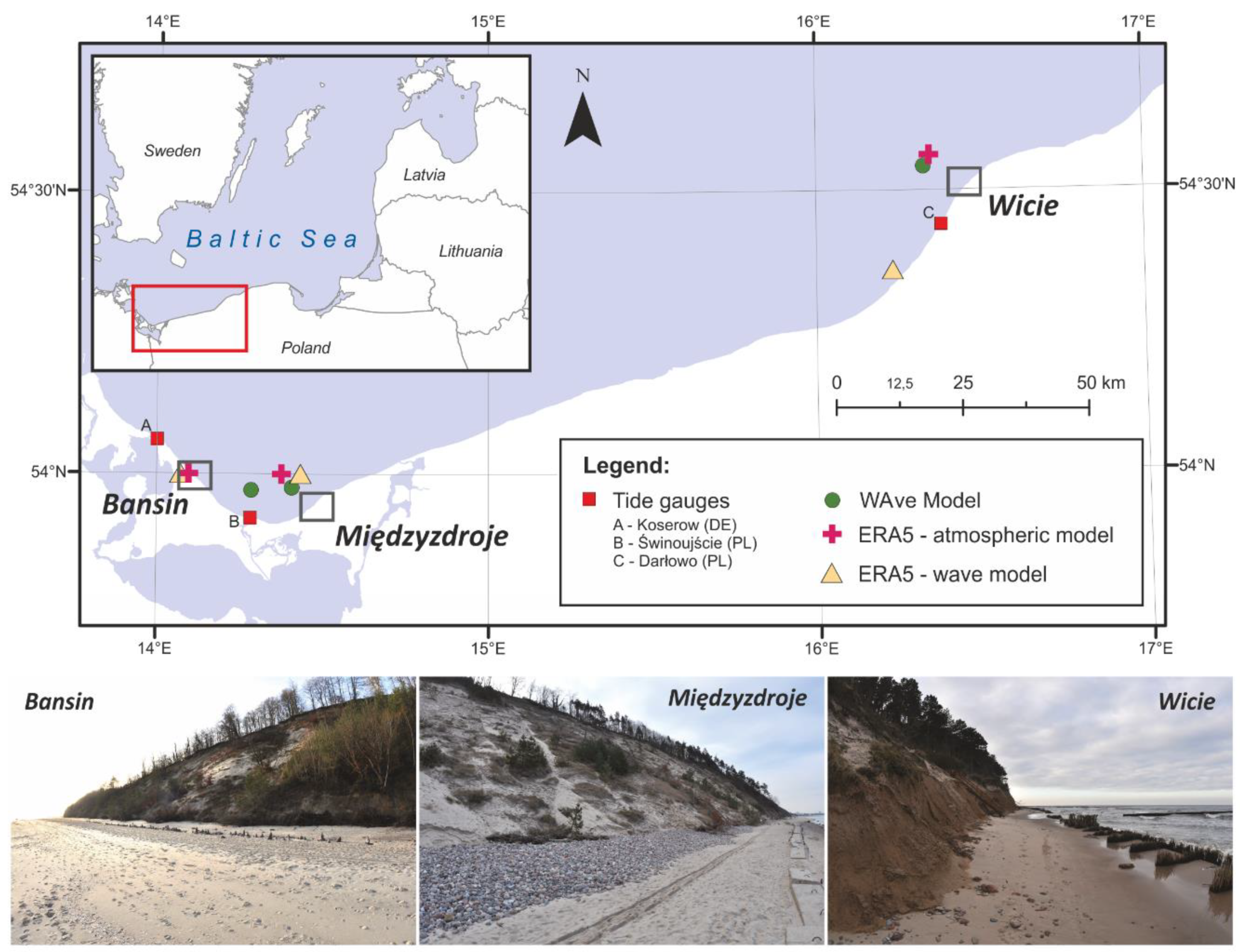
2.1. Study Sites

The cliff retreat analysis was performed for a non-tidal basin of the Baltic Sea (Figure 1). The Baltic Sea is dominated by winds from southwest and west directions. The prevailing directions in particular seasons are as follows: spring—east and northeast; summer—southwest and northwest; autumn—northwest; winter—north, south, southwest, and northwest. The highest strength of wind (> 6°B) reaches from November to March [20].
In recent decades, the highest absolute amplitude of sea level changes in the study area was recorded during year 1984 (2.79 m), whereas the most extreme storm surge occurred in November 1995 (+1.61 m above mean) [21]. However, extreme value analysis have shown that a 100-year storm surge in the western part of the Polish coast could reach +1.71 m above mean, and a 500-year event would exceed 2 m [22].
The study area covered three 500 m long cliff sites that have different geomorphological configurations. The first two research areas were located in Poland near two popular seaside resorts, Międzyzdroje (Wolin Island, Biała Góra cliffs) and Wicie, representing similar northwestern coastal exposures but with different geomorphological contexts. The third area was located in Germany next to the Bansin resort (Usedom Island, Langer Berg cliffs) and was characterized not only by different exposure (northeastern), but also by a much wider beach protecting the cliffs. Detailed in situ investigations were not performed for any of the analyzed cliff test sites.
The cliff formations selected to represent the effects of marine abrasion have long been subjects of widespread research interest. Moraine hills built of glacial and glaciofluvial deposits, till, and eolian deposition predominate the relief of these areas in which the landscape varies greatly from beaches to its characteristic element: high cliffs. This region is among the stormiest in Europe, experiencing high surges and strong winds [23]. The erosion rate has been frequently debated, as different rates are measured using a variety of techniques, either directly in the field (both with traditional and modern measurement techniques) or by analyzing historical maps [24].
The cliff coast of the Usedom Island, with the highest cliff (ca. 58 m) at this section named Streckelsberg, was subjected to largest coastal erosion in the area, endangering the town of Koserow, located partially on its stoss side. Generally Usedam Island cliff has been protected since the end of the 19th Century [25] by a cliff rampart, strengthened by a triple wall, groynes, three wave-breakers, and sand nourishment in modern times. For the study need a shorter, but unprotected by human made structures, an active cliff section of similar height (ca. 54 m) was chosen. This cliff, named Langer Berg, retreated ca. 100 m in 300 years [26] and is leaded by a sandy beach up to 30 meters wide.
As storms, wind, precipitation, and the sun contribute to the cliffs’ erosion the Wolin cliffs (ca. 90 m high in heights parts and ca. 57 m high in investigation site), the cliffs retreat approximately 80 cm per year, although the exact erosion rate is a subject that has been discussed for years [1,16,24]. The front of the high cliffs is protected by a series of flat concrete blocks, reaching up on average up to several meters, mostly covered by mix of sand and gravels beach, dogged deep into the sand and uncovered occasionally by strong storms [1].
The Wicie study site represents a slightly different geomorphological context. The beach in front of the cliffs is covered by mix of sand and gravels similarly to Międzyzdroje test site, but its width varies from less than 1 m to up to 20 m, depending of the analyzed section. The cliff face itself is much lower in highest sections, reaching only 11 m. The investigated area is protected by a series of manmade groins. No detailed geomorphological or geological investigations have been performed on this section of the Polish coast.

2.2. Data

The data used in this study covered a survey timeline from November 2016 to June 2018. Thirty-nine topographic surveys (thirteen for each study site) were conducted with terrestrial laser scanner (TLS) technology. The significant advantage of TLS data collection compared to traditional techniques or airborne laser scanning is related to time limitations. Coasts are extremely dynamic environments. To track cliff changes and identify the processes of its modifications, data must be collected frequently over consistent time intervals [27]. Data collection using classic field methods is a long and laborious process, which in the case of numerous and extensive research areas may not provide the required results. The implemented laser-based survey technique allowed for rapid and accurate collection of large amounts of topographic data. During the last decade, TLS has been successfully applied to topographic surveys and to the monitoring of coastal processes [28,29,30]. In this study, highly accurate measurements of coastal changes were performed with the use of Riegl VZ-400 equipment. Each of the 500 m long test sites were scanned from 10 spots, acquiring 90 to 100 points per square meter, with an estimated vertical accuracy of more than 5 mm. A list of all surveys and the resulting analytical periods is included in Supplementary Information 1 (Table S1).
The hydrometeorological data used in this study combined both observational and modeled datasets (Table 1). Wave parameters from the high-resolution operational WAve Model (WAM) were validated for the Baltic Sea in the framework of the Hindcast of dynamic processes of the ocean and coastal areas of Europe (HIPOCAS) project [31]. One minor gap lasting 6–7 h for two WAM points corresponding to the Bansin and Międzyzdroje cliffs was filled by interpolation. Three larger gaps in the wave and wind parameters for all locations, lasting a total of 36 days (within December 2016, June 2017, and February 2018), were filled using the fifth major global climate reanalysis dataset produced by the European Center for Medium-Range Weather Forecasts (ERA5) [32]. As the resolution of the ERA5 reanalysis model, which represents wave conditions further from the coast, is far coarser than the WAM data, the ERA5 values were corrected by a constant factor for each location, variable, and data gap. The constant factor was computed by dividing the average WAM values for the available days within each month during which a gap occurred by the average ERA5 reanalysis values.
Information on water levels was derived from tide gauges located at the shortest distance from each case study site through personal communication with the institutions responsible for the gauge upkeep. Finally, hourly precipitation and temperature data were collected from the ERA5 reanalysis model.

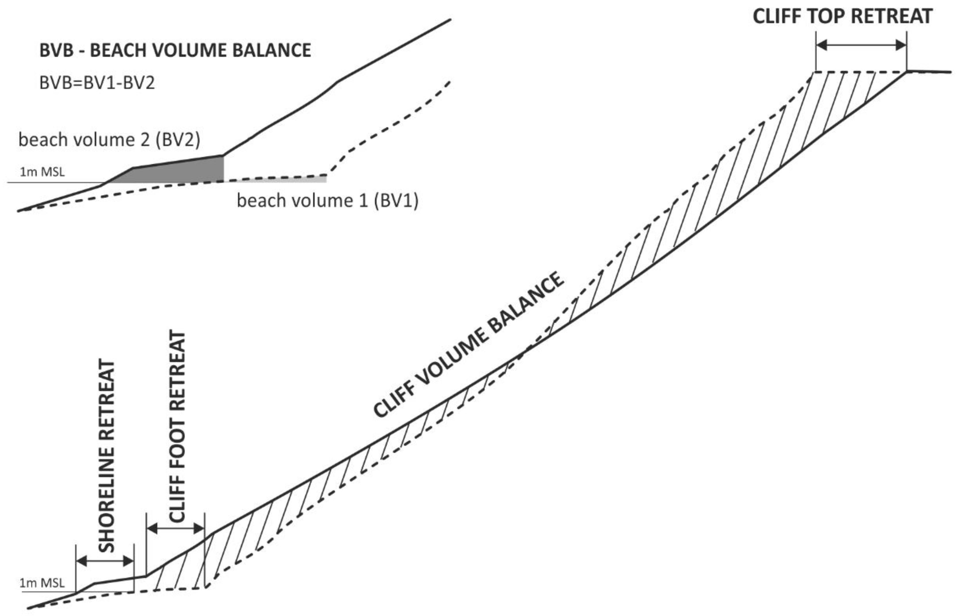
2.3. Geomorphological Indicators

Depending on the study objectives, five major geomorphological indicators were extracted from the LiDAR-derived digital elevation models (DEMs), namely shoreline retreat, beach volume balance, cliff foot retreat, cliff volume balance and cliff top retreat (Figure 2.). Because part of the topographic measurements were realized directly after storms while the water level was still quite high, some limitations in the high-resolution dataset availability caused the shoreline retreat indicator to be extracted as a 1 m contour above mean sea level (MSL) instead of at zero MSL.
Extracting the shoreline contour from DEM was rather straightforward; however, acquiring the cliff base line was more challenging and required some deliberation. Because the purpose of this study was to create reproducible solutions for analyzing the relationship between the erosion rates on coastal cliffs, a comparable procedure for extracting cliff base line was needed. While several studies realized on cliffs analyzed volumetric changes, to our knowledge, all assumed manual delineation of the cliff baseline, relying mainly on aerial photographs, topographic maps, or in situ surveys [1,18,33,34]. Some attempts of advanced automatic delineation were performed on the cliff bases of generalized coastal shoreline vectors by approximating the distance between shoreline and the cliff top [19]. In our study, a simplified methodology was implemented that considered a rapid change in altitude (higher than 0.5 m for a distance of 1 m). This procedure appeared to be a sufficient solution, because the delineation of the cliff base line can be a subject of interpretation, even by operators during field surveys. Moreover, as presented by Palaseanu-Lovejoy et al. [19], the manual digitization of geomorphological breaklines on DEMs not only has lower precision but also lacks reproducibility. The assumed simplified procedure was fully reproducible and comparable for all test sites and was a sufficient indicator that was independent of human skill.
Mapping the cliff top line and its migration over time is one of the most common methodologies for investigating cliff recession [24]. Traditionally obtained during field surveys or based on hand-digitized procedures [35], the cliff top line can also be extracted automatically [19]. Due to TLS limitations mainly related to data shortages on parts of the cliff edge densely overgrown by vegetation, the highest available point existing on two successive topographic surveys was assumed as the cliff top line for the analyzed time period.
Finally, to explore how the beach–cliff system changed between each LiDAR survey, line indicator migration as well as volumetric changes was analyzed. The results were separately determined for beach and cliff areas between the lines in 50 m wide sections. Similarly, for the needs of Bayesian network analysis, all line indicators were marked on profiles using the same 50 m spacing as the volumetric measurements.

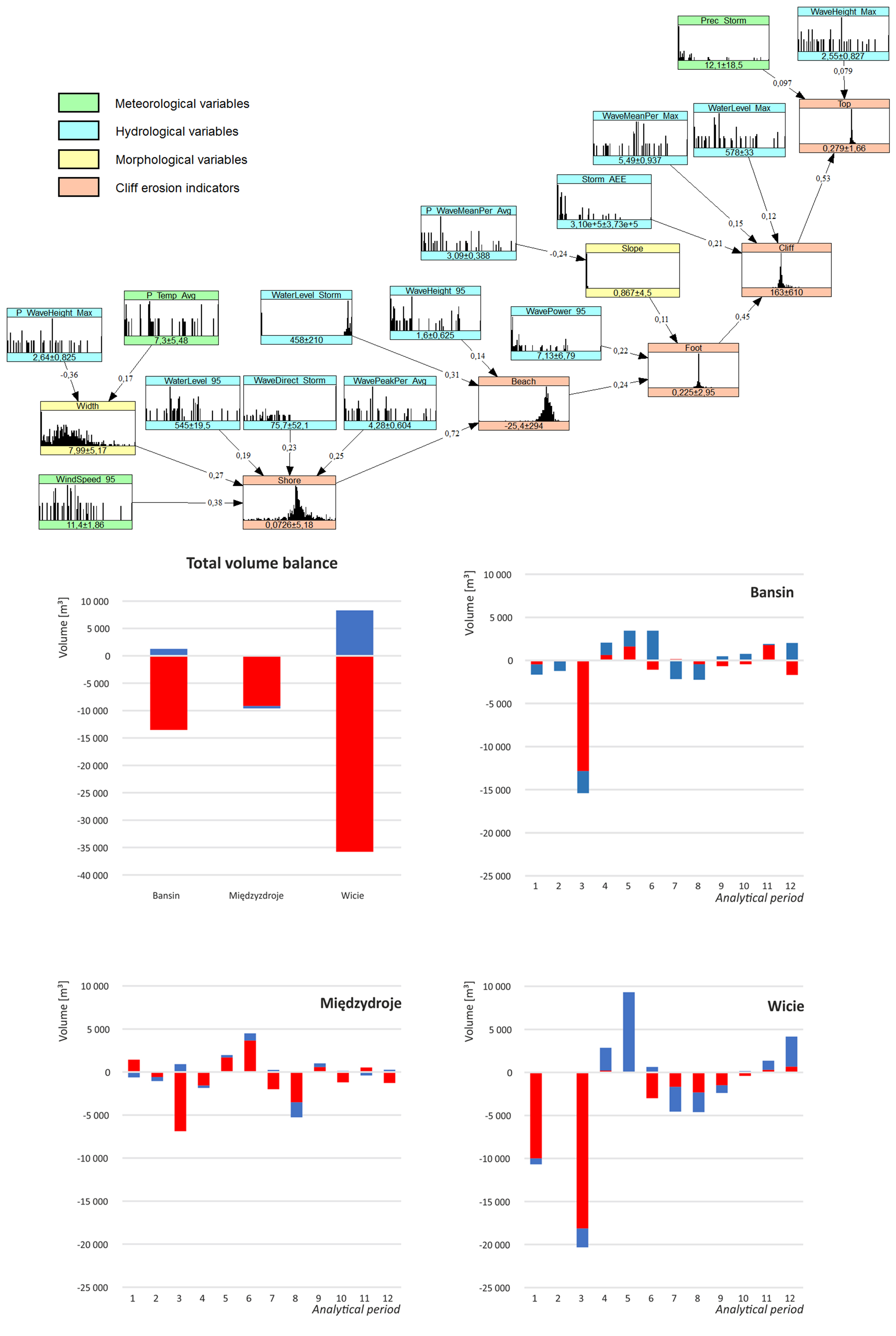
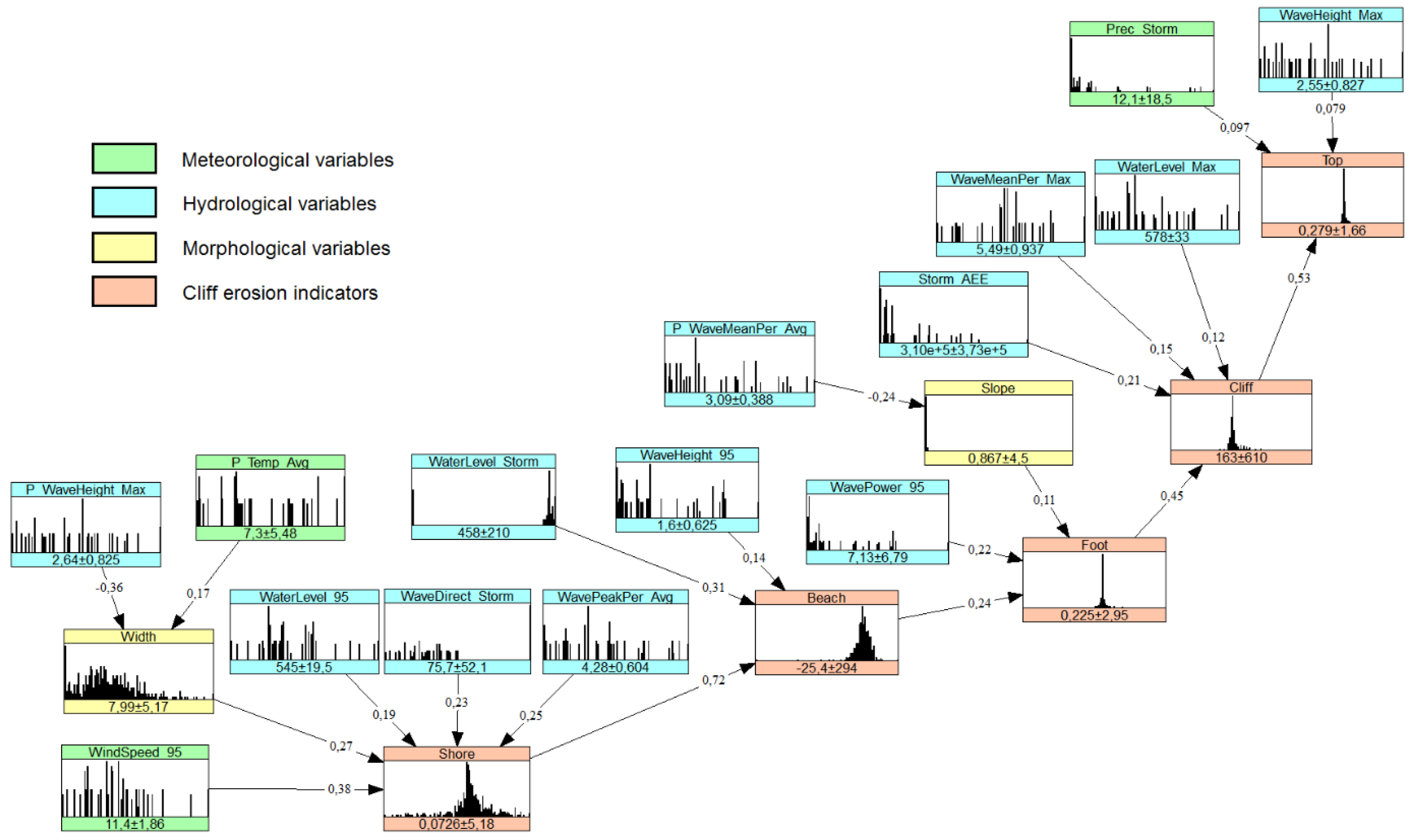
2.4. Bayesian Networks

Bayesian networks, also known as Bayesian belief nets, are graphical, probabilistic models [36] that have a wide range of applications in the environmental sciences, particularly in coastal zone problems [10,14]. The main advantage of BNs is the ability to model complex processes and, at least for models with a small number of nodes, the explicit representation of uncertainty and intuitive interpretation. BNs can be discrete or continuous, depending on the type of data available. In this study, a continuous BN was applied as it better suits the data collected (for discussion on pros and cons of various BN types, we refer to Hanea et al. [37]).
In general, a BN consists of a directed acyclic graph with associated conditional probability distributions [38,39]. The graph consists of “nodes” and “arcs” in which the nodes represent random variables connected by arcs, which represent the dependencies between variables. Arcs have a defined direction: the node on the upper end is known as the “parent” node, and the node on the lower (receiving) end is the “child” node. Each variable is conditionally independent of all predecessors given its parents: if one conditionalizes the parent node and there is no arc connecting the child node with any of the predecessors of the parent node (directly or through another parent node), the conditional distribution of the child node does not change if the predecessors of the parent node are conditionalized. The joint probability density f(x_1,x_2,…,x_n) for a given node is therefore written as
f ( x 1 , x 2 , , x n ) = i = 1 n f ( x i | x p a ( i ) )
where pa(i) is the set of parent nodes of X_i. One possibility of BNs is to update the probability distribution of child nodes given the new evidence at parent nodes. Two elements are needed to quantify a BN: the marginal distribution for each node and a dependency model for each arc. In this study, we used non-parametric margins, which were the same as the empirical distribution of data collected for this study. The dependencies were represented by normal (Gaussian) copulas. Basically, a copula is a joint distribution on the unit hypercube with uniform (0,1) margins. While there are many types of copulas (we refer to Joe [39] for detailed descriptions), the assumption of a normal copula is a limitation of the available computer code [38]—though most dependencies between variables used here did not indicate tail dependence—a property that can be represented as either normal, Frank, or Plackett copulas. A goodness-of-fit test for copulas proposed by Genest et al. [40] indicates that several copula types are, on average, similarly suitable for the analysis (Frank, Plackett, t, Gumbel, Gaussian), while others much less (Clayton and Joe copulas). A normal copula was parameterized using Spearman’s rank correlation coefficient; hence, in all cases, the results refer to this measure of correlation. For the detailed procedure of obtaining conditional probabilities from a non-parametric continuous BN with a normal copula, we followed the procedure of Hanea et al. [37]. The algorithms from that study were implemented in the Uninet software used to build our model.
The configuration of nodes and arcs is researcher dependent. Yet a good BN incorporates existing knowledge of the process in question, in this case the factors influencing the cliff erosion and the physical processes in action. For this study, a total of 41 variables were tested while preparing the BN. The full list of variables and their descriptions is available in the SI1 file. Five erosion indicators (Section 2.3) and two further geomorphological indicators, namely beach width (i.e., between shoreline and cliff foot) and cliff slope (i.e., above cliff foot), were used as variables. The following rules were used to design the BN model in this study:
  • Cliff erosion indicators were connected with each other, starting from the shoreline retreat indicator and moving toward the cliff top.
  • In every case, the cliff erosion indicator was used as the first parent node when other parent nodes were added.
  • Meteorological, hydrological, and morphological variables were added starting from the shoreline retreat (Shore) node and moving toward the cliff top.
  • Each variable was connected only to one node containing a cliff erosion indicator.
  • Meteorological and hydrological variables were not given any parent nodes and were not connected with each other.
  • The first meteorological or hydrological variable to be connected with a cliff erosion indictor was the variable with the highest unconditional correlation within the model. The unconditional correlation matrix is shown in Supplementary Information 2.
  • Further meteorological or hydrological variables were selected based on the conditional correlation with cliff erosion indicators.
  • Only parent nodes with (conditional) correlations higher than 0.1 were included in the model, except for the parents of cliff top retreat (Top), where only the correlation with the cliff volume balance (Cliff) exceeded this threshold.
The meteorological and hydrological factors, such as significant wave height, wave direction, mean wave period, peak wave period, water level, wind speed, temperature, and precipitation, were used in several configurations where applicable: mean (total), maximum (minimum) values between measurement campaigns, mean value during storm surges, and the 95th (5th) percentile during the period between measurement campaigns. Synthetic indicators of storm conditions were also investigated, including storm energy [41], accumulated excess energy [42], and wave power [43]. For the purposes of this study, a storm surge was defined as a water level of at least 0.45 m above mean sea level (545 cm Normal Null); this value was selected on the basis of (unconditional) correlations between erosion and hydrological variables. Moreover, if after a storm, the water level fell below this level for less than 6 h before the next storm, the whole series was considered to be one storm surge. The value of the upper and lower percentile in some indicators was similarly selected to maximize (unconditional) correlations across multiple variables.

3. Results

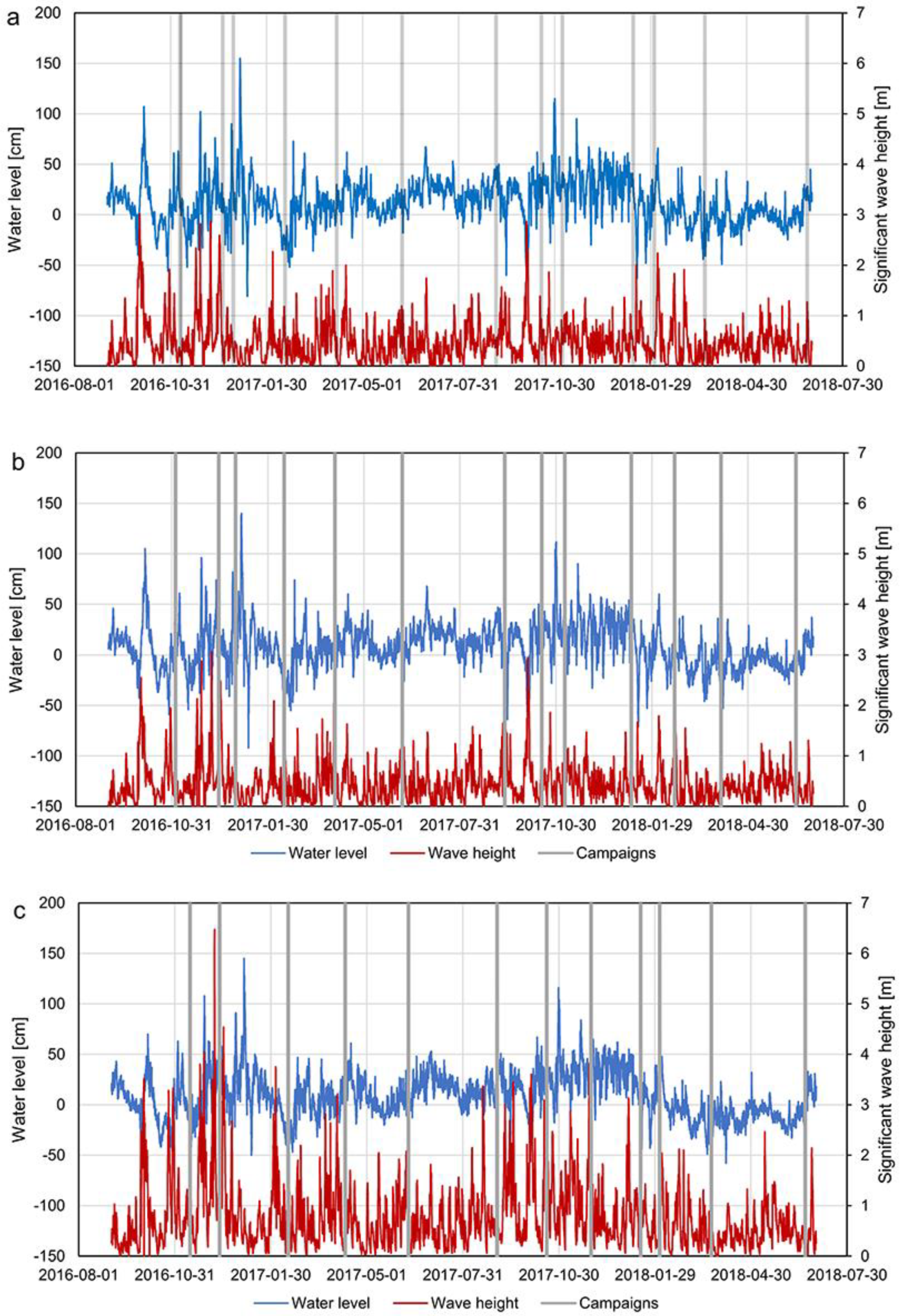
3.1. Hydrological Conditions during the Period of Study

Many storms reached the coast during the measurement period. Using the definition of storm surge described in Section 2.4 (based on sea levels of at least 0.45 m above mean sea level), a total of 61 storms affected the cliffs in Bansin, compared to 43 in Międzyzdroje and 62 in Wicie. The distribution of surges was highly uneven, as shown in Figure 3. The most intense period lasted from late November 2016 to mid-January 2017. Around 10 surges were distinguished during that period, with water levels exceeding 1.4 m above average at all locations on 4–5 January 2017. This water level corresponded to an event with a return period of 15–20 years [44]. The maximum water level of 1.55 m was observed at the Koserow tide gauge close to the Bansin cliffs. Conversely, the waves reached their maximum height throughout late 2016, culminating on 7 December 2016.
Another period of stormy weather lasted from mid-October 2017 to early January 2018, during which around 20 surges affected the coast. However, neither the water levels nor the wave heights were as extreme as those during the 2016–2017 storm season. The most intense storm in the 2017–2018 storm season occurred around 29–30 October 2017 during which the water levels slightly exceeded 1 m above mean in all study areas. Considering the stricter definition of storm surge presented by Wiśniewski and Wolski [44], i.e., the exceedance of water levels of 0.6 m above mean, the first half of the study period had three times more storms than the long-term average of about four per year, including a very unusual occurrence of a storm surge in June; the second half of the study period was close to an average year.

3.2. Descriptive Analysis of Cliff Erosion

During the monitoring period, the sediment budget was definitely negative with a total loss of 49,330 m3. Erosion was most significant on the cliffs (over 58,000 m3), while a positive budget was observed on the beaches, with a value slightly exceeding 9000 m3. This positive balance shows that not all of the cliffs’ material was swept into the sea, but some of it remained on the beaches.
Erosion and sedimentation were unevenly distributed in time and space (Figure 4). At the beginning of the 2016–2017 storm season, erosion was principally visible on the beach (over 80% of total erosion volume in Bansin and Międzyzdroje). As the successive lowering of beach proceeded, the proportions changed, and the cliff erosion started to dominate, reaching over 85% of the total erosion volume. Due to the very narrow beach, the Wicie area suffered cliff-dominated erosion of more than 90% of the total loss in this coast section. In fact, the sediment budget was obviously negative both for the beach and cliff during the winter season. The maximum negative volume of eroded material measured between the third and fourth topographic campaigns was also the highest during the monitoring period. Erosion volume on the beach varied at different test sites, reaching from 627 to 2191 and 2566 m3 for Międzyzdroje, Bansin, and Wicie beaches, respectively. However, the first group of severe storms affected the cliff face much stronger than the beach, exceeding the maximum volumes of 6000, 12,000, and 18,000 m3 for Międzyzdroje, Bansin, and Wicie cliffs, respectively. Notwithstanding the clear erosion dominance across the whole study area during the 2016–2017 storm season, the retreat of the cliff top was relatively small compared to changes of the 1 m contour line and the cliff base line. While the cliff top retreated by a maximum of 11 m in Wicie, the average change on all areas was less than 1 m, and the median was only 0.03 m. The maximum changes of shoreline and cliff base lines were similar, reaching around 11 m. However, the average change of shoreline and cliff base lines of 2.5 and 1.3 m, respectively, as well as medians of 1.7 and 0.15 m, respectively, suggested more even distribution.
The period between storm seasons contained higher variability in both the time and space distributions, even though the total volumes were much lower. Furthermore, the compilation of the next five surveys revealed both accumulation and erosional patterns with a rather modest positive overall sediment budget (1800 m3). Before the 2017 winter season approached, the dominant processes were much weaker, but cliff erosion still occurred along with the overall recovery of beach height and length. The volume values between surveys fluctuated from –2870 to 9280 m3 and –3520 to 3683 m3, respectively, for beach and cliff. However, the negative values for the beach and the positive for the cliffs were a consequence of landslide processes that pushed the cliff base line in the seaward direction rather than significant erosion or deposition episodes.
The second period of stormy weather as well as the following spring season (2017–2018) revealed strong similarities to the corresponding earlier periods. This observation was supported by a comparison of data from the last four topographic surveys. Erosion was still principally visible on the cliffs, though the water levels and wave heights were not as extreme as those during the 2016–2017 storm season. The much weaker waves were not able to clean all the debris, and in some of the investigated areas, the cliff base line migrated seawards, and the volume values presented an inverse pattern to what was observed during the first storm season. The after-storm period was again characterized by beach recovery processes.

3.3. Statistical Analysis of Cliff Erosion

The statistical analysis was performed using the BN presented in Figure 5. The final model, constructed following the procedure explained in Section 2.4., included five cliff erosion indicators explained by two morphological factors, eleven hydrological factors, and two meteorological factors. The morphological factors were additionally explained by two hydrological factors and one meteorological factor.
The shoreline is the most dynamic component of the coastline; therefore, its changes (Shore) have the highest number of explanatory variables. The highest correlation was observed with the 95th percentile of wind speed (WindSpeed_95), which gave a slightly higher correlation than the wave height indicators. A likely explanation for this relationship is that wind is more dynamic than offshore waves containing significant inertia and hence is a better predictor of the small wind-driven waves that contribute to shoreline retreat. The second factor influencing shoreline retreat was the width of the beach (Width) before the occurrence of erosion. Wider beaches have more material to be eroded, resulting in larger shoreline retreat. The beach width was influenced by both the maximum wave height (P_WaveHeight_Max), which resulted in shorter beaches, and the average temperature (P_Temp_Avg), which is an indicator of the time of the year, as beaches tend to be shorter during the autumn and winter storm season than during the warmer spring or summer. Other factors contributing to shoreline retreat were the 95th percentile of water levels (WaterLevel_95), average wave direction during storm surges (WaveDirect_Storm), and average wave peak period (WavePeakPer_Avg), all of which resulted in higher and longer waves attacking the shoreline, resulting in erosion.
Beach volume balance (Beach) was highly correlated (0.72) with shoreline retreat, which incorporated the influence of several factors. The average water level during storms (WaterLevel_Storm) further contributed to beach erosion, as higher baseline sea levels allowed waves to reach further onto the beach, while the 95th percentile of significant wave height (WaveHeight_95) indicated the importance of high waves in beach erosion.
Cliff foot retreat (Foot) showed a relatively low correlation (0.24) with beach volume balance, as more complex mechanisms were observed: material from cliff erosion could be deposited on the beach, which would result in a weak dependency between beach and cliff erosion. However, some of the waves eroding the beach still cut into the cliff. Specifically, waves that were both particularly high and long contributed to cliff foot retreat, as revealed by the wave power (WavePower_95) indicator, which was proportional to the product of significant wave height and the mean wave period. Additionally, the cliff was more prone to erosion if more vertical than inclined, as shown by the cliff slope (Slope) variable. The cliff slope showed the highest correlation with the average mean wave period in the preceding period (P_WaveMeanPer_Avg), where stormy periods resulted in lower cliff slopes due to erosion.
The cliff volume balance (Cliff) depended primarily on waves undercutting the cliff, resulting in the eventual collapse of the cliff. Erosion was further increased by very high waves, as shown by the accumulated excess energy (Storm_AEE) indicator. The accumulated excess energy indicator represented the energy of waves above a 2 m threshold (including sea level), which was close to the average elevation of cliff foots in the study area; hence, this indicator counted only the waves that actually eroded the cliff. Two other variables correlated with the cliff volume balance were the maximum mean wave period (WaveMeanPer_Max), which indicated the occurrence of very long waves, and the maximum water level (WaterLevel_Max), as the high baseline sea level increased the number of waves that could reach the cliff.
Finally, erosion of the cliff could also result in retreat of the cliff top (Top). This erosion indicator was the least dynamic and depended mostly on factors already included in previous erosion indicators. Some correlation existed with the total precipitation recorded during storms (Prec_Storm), as rainfall could weaken the structure of the cliff, making it more susceptible to collapse. Other factors showed only a small conditional correlation; the largest was for the maximum wave height (WaveHeight_Max), which indicated the occurrence of extreme waves having the biggest impact on the cliff.
The model was validated by analyzing the correlation between predicted and observed changes in the variables of interest (Table 2). This was carried out for different choices of input sample, thus analyzing how transferable is the model between locations. The small sample size resulted in a non-negligible variation of results between different model runs; therefore, the results shown are averages of 100 model runs per each variant of location or sample source. A split-sample validation (using half of the data as input sample, and the other half to run the model) showed only marginally lower performance than using the same data for both purposes. Of the three study sites, data from the Bansin cliff is the most transferable. For individual variables, the highest correlation between modeled and observed data is for beach volume balance, followed by shoreline retreat and beach width (correlations of 0.4-0.6). Correlations for cliff foot and volume balance are in the 0.3–0.4 range, and lower for the cliff top, which was the least dynamic part of the cliff in the timeframe of the study.

4. Discussion

The tracking of cliff changes requires very detailed topographic data to be acquired repeatedly in time, not only for revealing patterns of coastal behavior [18,45] but also for providing better understanding of the relations between processes and indicators. As the comparison of two datasets provided only a cumulative result for coastal analysis [15,16], multiple measurements enabled the analysis of both isolated events and storm series on erosion, as well as the processes for cliff modifications.
In this study, we demonstrated that changes to coastal cliffs are very complex, and physical processes that influenced both beach and cliff may be responsible for erosion processes. Our results confirmed the impact of sea activity as well as enabled evaluation of the effects of unfavorable weather conditions to coastal cliffs [18,24]. In fact, the cliff coast develops as a result of numerous overlapping processes. While storm surges undercut and destabilize cliff faces [46], waves are mainly responsible for temporal shoreline changes with correlation to temperature, which acts as a season indicator. Consequently, the beach is successively eroded and lowered, resulting in the occurrence of favorable hydrometeorological conditions for cliff erosion. These conditions are not directly linked to the highest waves, but to longest waves during maximum water levels. While high-magnitude events advance cliff face erosion, when these events weaken, part of the transported debris is lost, which starts the process of beach recovery [47,48]. Finally, the most powerful events were not able to directly influence the cliff top line. As presented by Kostrzewski et al. [24], changes of the cliff top line are linked with precipitation factors, especially during storm events.
In this study, as suggested by Andrews et al. [27], numerous topographic “snapshots” realized more than several times during a year were analyzed with increasingly popular Bayesian networks. This analysis enabled an understanding of the complex changes of coastal systems from the event scale to seasonal variations. The BN model presented here is the first BN application for analyzing short-term cliff erosion and therefore is not comparable with the few existing models due to the different spatial or temporal scales and model designs. Some similarities could be found; however, as certain common factors were identified to contribute to erosion, such as the cliff/beach slope, sea level, and wave height. On the other hand, recurring variables were not included in this study, such as the tidal range and geology/geomorphology of the coast. Tides have negligible amplitude along the coast in question. The qualitative properties of the cliffs were not included due to the similarity of the study sites. Moreover, inclusion of the geomorphology would necessitate the use of a discrete or hybrid BN, which would require a very different model set up in the context of our relatively small sample size.
In this study, the model was used for data analysis without making predictions. The inclusion of prediction capability in our model would require validation based on another cliff erosion dataset. For instance, the annual cliff top erosion since 1985 for multiple sections of the Wolin Island cliffs [24] could be used for this purpose. However, such an analysis is limited by the availability of hydrometeorological data. Existing reanalyses (ERA5, ERA-Interim) have much lower resolution than the WAM model used here; therefore, the wave conditions indicated in those reanalyses differ substantially from those in WAM: they show much bigger wave heights. Moreover, tests with an operational BN model have shown that such models are too sensitive, given the amount of data available. Therefore, more LiDAR scanning campaigns performed would be needed to improve the performance of the model, especially for the less dynamic upper parts of the cliff. The model than could be reworked using ERA5 as the input hydrometeorological dataset, which planned to be extended back to 1950 [32]. Moreover, the assumption of a normal copula for modeling the dependencies would need to be validated before the model could be used for prediction [49], and the graph would need to be further investigated to better represent the joint distribution [50]. The SI1 file presents an example of a modified BN with many additional arcs between the hydrometeorological variables, as those are the most highly correlated, and such connections are relevant for properly representing the joint distribution.

5. Conclusions

  • Our study demonstrates the advantages of using Bayesian network for analysis of surface morphological changes on cliff coasts even on relatively short analyzed shore segments. Despite the site-specific geomorphological settings for different test areas, the implementation of the proposed Bayesian network model enabled the determination of relationships between the erosion rates and selected factors. The proposed model explained the general behavior of the cliff coast with respect to different hydrometeorological conditions, indicating variables most relevant at each segment along the profile. Validation of the model showed good performance along the beach and cliff foot, but weaker in predicting cliff mass balance or cliff top recession.
  • Our study proves that high temporal resolution in TLS surveys enables the analysis of correlations between the influence of several factors (wave height, length and period, water level, storm energy, precipitation, etc.) and the geomorphological response of coast during isolated storm events, as well as with cumulative effects for season-long analysis. In general, a presentation of short and mid-term analyses expands possibilities in coastal morphological studies. Although we have seen a rapid increase of TLS usage in recent years, most of these have focused on a small quantity of realized surveys or long-term analysis.
  • The automatic extraction of all geomorphological indicators from DEMs enabled reproducible and comparable cliff recession analysis. However, caution should be taken when interpreting the beach recovery, because some erosion and deposition processes may be masked by an automatic delineation of the cliff base line.

Supplementary Materials

The following are available online at https://0-www-mdpi-com.brum.beds.ac.uk/2072-4292/11/7/843/s1: Table S1.1. Analytical periods used in the study according to dates of surveys by test site, Table S1.2. Candidate variables for the Bayesian Network model and their description, Description S1. Equations of synthetic indicators, Figure S1.1. A Bayesian Network for cliff erosion witb additional arc between hydrometeorological variables, Figure S1.2. D-calibration score for the unsaturated BN from the paper, Figure S1.3. D-calibration score for the saturated BN from this supplement. The following are available online at https://0-www-mdpi-com.brum.beds.ac.uk/2072-4292/11/7/843/s2: Table S2.1. Spearman’s rank correlations.

Author Contributions

Conceptualization, methodology, formal analysis and writing original draft: P.T. and D.P.; writing – review and editing: P.T., D.P. and A.G.; data curation: P.T., A.G.; resources and visualization: A.G. and S.W.; validation D.P.; supervision: O.M-N. and A.K; funding acquisition: P.T.

Funding

This research was funded by the National Science Centre, Poland, grant number UMO-2015/17/D/ST10/02191 “Coastal cliffs under retreat imposed by different forcing processes in multiple timescales - CLIFFREAT”.

Conflicts of Interest

The authors declare no conflict of interest.

References

  1. Terefenko, P.; Giza, A.; Paprotny, D.; Kubicki, A.; Winowski, M. Cliff retreat induced by series of storms at Międzyzdroje (Poland). J. Coastal Res. 2018, 85, 181–185. [Google Scholar] [CrossRef]
  2. Furmańczyk, K.; Andrzejewski, P.; Benedyczak, R.; Bugajny, N.; Cieszyński, Ł.; Dudzińska-Nowak, J.; Giza, A.; Paprotny, D.; Terefenko, P.; Zawiślak, T. Recording of selected effects and hazards caused by current and expected storm events in the Baltic Sea coastal zone. J. Coastal Res. 2014, 70, 338–342. [Google Scholar] [CrossRef]
  3. Paprotny, D.; Andrzejewski, P.; Terefenko, P.; Furmańczyk, K. Application of Empirical Wave Run-Up Formulas to the Polish Baltic Sea Coast. PLoS ONE 2014, 9, e105437. [Google Scholar] [CrossRef] [PubMed]
  4. Bugajny, N.; Furmańczyk, K. Comparison of Short-Term Changes Caused by Storms along Natural and Protected Sections of the Dziwnow Spit, Southern Baltic Coast. J. Coastal Res. 2017, 33, 775–785. [Google Scholar] [CrossRef]
  5. Deng, J.; Harff, J.; Zhang, W.; Schneider, R.; Dudzińska-Nowak, J.; Giza, A.; Terefenko, P.; Furmańczyk, K. The Dynamic Equilibrium Shore Model for the Reconstruction and Future Projection of Coastal Morphodynamics. In Coastline Changes of the Baltic Sea from South to East; Harff, J., Furmańczyk, K., VonStorch, H., Eds.; Springer: Cham, Switzerland, 2017; pp. 87–106. [Google Scholar]
  6. Uścinowicz, G.; Szarafin, T. Short-term prognosis of development of barrier-type coasts (Southern Baltic Sea). Ocean Coast. Manag. 2018, 165, 258–267. [Google Scholar] [CrossRef]
  7. Prémaillon, M.; Regard, V.; Dewez, T.J.B.; Auda, Y. GlobR2C2 (Global Recession Rates of Coastal Cliffs): A global relational database to investigate coastal rocky cliff erosion rate variations. Earth Surf. Dyn. 2018, 6, 651–668. [Google Scholar] [CrossRef]
  8. Hall, J.W.; Meadowcroft, I.C.; Lee, E.M.; van Gelder, P.H.A.J.M. Stochastic simulation of episodic soft coastal cliff recession. Coast. Eng. 2002, 46, 159–174. [Google Scholar] [CrossRef]
  9. Le Cozannet, G.; Garcin, M.; Yates, M.; Idier, D.; Meyssignac, B. Approaches to evaluate the recent impacts of sea-level rise on shoreline changes. Earth-Sci. Rev. 2014, 138, 47–60. [Google Scholar] [CrossRef] [Green Version]
  10. Beuzen, T.; Splinter, K.D.; Marshall, L.A.; Turner, I.L.; Harley, M.D.; Palmsten, M.L. Bayesian Networks in coastal engineering: 5 Distinguishing descriptive and predictive applications. Coast. Eng. 2018, 135, 16–30. [Google Scholar] [CrossRef]
  11. Hapke, C.; Plant, N. Predicting coastal cliff erosion using a Bayesian probabilistic model. Mar. Geol. 2010, 278, 140–149. [Google Scholar] [CrossRef] [Green Version]
  12. Gutierrez, B.T.; Plant, N.G.; Thieler, E.R. A Bayesian network to predict coastal vulnerability to sea level rise. J. Geophys. Res. 2011, 116, F02009. [Google Scholar] [CrossRef]
  13. Yates, M.L.; Le Cozannet, G. Brief communication “Evaluating European Coastal Evolution using Bayesian Networks”. Nat. Hazards Earth Syst. Sci. 2012, 12, 1173–1177. [Google Scholar] [CrossRef]
  14. Jäger, W.S.; Christie, E.K.; Hanea, A.M.; den Heijer, C.; Spencer, T. A Bayesian network approach for coastal risk analysis and decision making. Coast. Eng. 2018, 134, 48–61. [Google Scholar] [CrossRef]
  15. Le Mauff, B.; Juigner, M.; Ba, A.; Robin, M.; Launeau, P.; Fattal, P. Coastal monitoring solutions of the geomorphological response of beach-dune systems using multi-temporal LiDAR datasets (Vendee coast, France). Geomorphology 2018, 304, 121–140. [Google Scholar] [CrossRef]
  16. Kolander, R.; Morche, D.; Bimböse, M. Quantification of moraine cliff erosion on Wolin Island (Baltic Sea, northwest Poland. Baltica 2016, 26, 37–44. [Google Scholar] [CrossRef]
  17. Nunes, M.; Ferreira, O.; Loureiro, C.; Baily, B. Beach and cliff retreat induced by storm groups at Forte Novo, Algarve (Portugal). J. Coastal Res. 2011, 64, 795–799. [Google Scholar]
  18. Warrick, J.A.; Ritchie, A.C.; Adelman, G.; Adelman, K.; Limber, P.W. New techniques to measure cliff change form historical oblique aerial photographs and structure-for-motion photogrammetry. J. Coastal Res. 2017, 33, 39–55. [Google Scholar] [CrossRef]
  19. Palaseanu-Lovejoy, M.; Danielson, J.; Thatcher, C.; Foxgrover, A.; Barnard, P.; Brock, J.; Young, A. Automatic Delineation of Seacliff Limits using Lidar-derived High-resolution DEMs in Southern California. J. Coastal Res. 2016, 76, 162–173. [Google Scholar] [CrossRef] [Green Version]
  20. Rokiciński, K. Geograficzna i hydrometeorologiczna charakterystyka Morza Bałtyckiego jako obszaru prowadzenia działań asymetrycznych. Zeszyty Naukowe Akad. Marynarki Wojennej 2007, 48, 65–82. [Google Scholar]
  21. Wolski, T.; Wiśniewski, B.; Giza, A.; Kowalewska-Kalkowska, H.; Boman, H.; Grabbi-Kaiv, S.; Hammarklint, T.; Holfort, J.; Lydeikaitė, Ž. Extreme sea levels at selected stations on the Baltic Sea coast. Oceanologia 2014, 56, 259–290. [Google Scholar] [CrossRef]
  22. Paprotny, D.; Terefenko, P. New estimates of potential impacts of sea level rise and coastal floods in Poland. Nat. Hazards 2017, 85, 1249–1277. [Google Scholar] [CrossRef]
  23. Vousdoukas, M.I.; Voukouvalas, E.; Annunziato, A.; Giardino, A.; Feyen, L. Projections of extreme storm surge levels along Europe. Clim. Dyn. 2016, 47, 3171–3190. [Google Scholar] [CrossRef] [Green Version]
  24. Kostrzewski, A.; Zwoliński, Z.; Winowski, M.; Tylkowski, J.; Samołyk, M. Cliff top recession rate and cliff hazards for the sea coast of Wolin Island (Southern Baltic). Baltica 2015, 28, 109–120. [Google Scholar] [CrossRef] [Green Version]
  25. Schumacher, W. Coastal dynamics and coastal protection of the Island of Usedom. Greifswalder Geogr. Arbeiten 2002, 27, 131–134. [Google Scholar]
  26. Schwarzer, K.; Diesing, M.; Larson, M.; Niedermeyer, R.O.; Schumacher, W.; Furmanczyk, K. Coastline evolution at different time scales: Examples from the Pomeranian Bight, southern Baltic Sea. Mar. Geol. 2003, 194, 79–101. [Google Scholar] [CrossRef]
  27. Andrews, B.P.; Gares, P.A.; Colby, J.B. Techniques for GIS modeling of coastal dunes. Geomorphology 2002, 48, 289–308. [Google Scholar] [CrossRef] [Green Version]
  28. Vousdoukas, M.; Kirupakaramoorthy, T.; Oumeraci, H.; de la Torre, M.; Wübbold, F.; Wagner, B.; Schimmels, S. The role of combined laser scanning and video techniques in monitoring wave-by-wave swash zone processes. Coast. Eng. 2014, 83, 150–165. [Google Scholar] [CrossRef]
  29. Almeida, L.P.; Masselink, G.; Russell, P.E.; Davidson, M.A. Observations of gravel beach dynamics during high energy wave conditions using a laser scanner. Geomorphology 2015, 228, 15–27. [Google Scholar] [CrossRef] [Green Version]
  30. Terefenko, P.; Zelaya Wziątek, D.; Dalyot, S.; Boski, T.; Pinheiro Lima-Filho, F. A High-Precision LiDAR-Based Method for Surveying and Classifying Coastal Notches. ISPRS Int. J. Geo-Inf. 2018, 7, 295. [Google Scholar] [CrossRef]
  31. Cieślikiewicz, W.; Paplińska-Swerpel, B. A 44-year hindcast of wind wave fields over the Baltic Sea. J. Coastal Eng. 2008, 55, 894–905. [Google Scholar] [CrossRef]
  32. Hersbach, H.; Dee, D. ERA5 Reanalysis Is in Production. 2016. Available online: https://www.ecmwf.int/en/newsletter/147/news/era5-reanalysis-production (accessed on 23 November 2018).
  33. Rosser, N.J.; Brain, M.J.; Petley, D.N.; Lim, M.; Norman, E.C. Coastline retreat via progressive failure of rocky coastal cliffs. Geology 2013, 41, 939–942. [Google Scholar] [CrossRef] [Green Version]
  34. Johnstone, E.; Raymond, J.; Olsen, J.M.; Driscoll, N. Morphological Expressions of Coastal Cliff Erosion Processes in San Diego County. J. Coastal Res. 2016, 76, 174–184. [Google Scholar] [CrossRef] [Green Version]
  35. Hapke, C.J.; Reid, D. National Assessment of Shoreline Change, Part 4: Historical Coastal Cliff Retreat along the California Coast; USGS Open-File Report 2007-1133; U.S. Department of the Interior, U.S. Geological Survey: Santa Cruz, USA, 2007; 51p.
  36. Kurowicka, D.; Cooke, R. Uncertainty Analysis with High Dimensional Dependence Modelling; John Wiley & Sons Ltd.: Chichester, UK, 2006. [Google Scholar]
  37. Hanea, A.M.; Kurowicka, D.; Cooke, R.M. Hybrid Method for Quantifying and Analyzing Bayesian Belief Nets. Qual. Reliab. Eng. Int. 2006, 22, 709–729. [Google Scholar] [CrossRef]
  38. Hanea, A.; Morales Nápoles, O.; Dan Ababei, D. Non-parametric Bayesian networks: Improving theory and reviewing applications. Reliab. Eng. Sys. Saf. 2015, 144, 265–284. [Google Scholar] [CrossRef]
  39. Joe, H. Dependence Modeling with Copulas; Chapman & Hall/CRC: London, UK, 2014. [Google Scholar]
  40. Genest, C.; Rémillard, B.; Beaudoin, D. Goodness-of-fit tests for copulas: A review and a power study. Insur. Math. Econ. 2009, 44, 199–213. [Google Scholar] [CrossRef]
  41. Furmańczyk, K.K.; Dudzińska-Nowak, J.; Furmańczyk, K.A.; Paplińska-Swerpel, B.; Brzezowska, N. Critical storm thresholds for the generation of significant dune erosion at Dziwnow Spit, Poland. Geomorphology 2012, 143, 62–68. [Google Scholar] [CrossRef]
  42. Hackney, C.; Darby, S.E.; Leyland, J. Modelling the response of soft cliffs to climate change: A statistical, process-response model using accumulated excess energy. Geomorphology 2013, 187, 108–121. [Google Scholar] [CrossRef]
  43. Earlie, C.; Masselink, G.; Russell, P. The role of beach morphology on coastal cliff erosion under extreme waves. Earth Surf. Process. Landf. 2018, 43, 1213–1228. [Google Scholar] [CrossRef] [Green Version]
  44. Wiśniewski, B.; Wolski, T. Katalogi Wezbrań i Obniżeń Sztormowych Poziomów Morza oraz Ekstremalne Poziomy wód na Polskim Wybrzeżu; Maritime University of Szczecin: Szczecin, Poland, 2009. [Google Scholar]
  45. Young, A.P. Recent deep-seated coastal landsliding at San Onofre State Beach, California. Geomorphology 2015, 228, 200–212. [Google Scholar] [CrossRef]
  46. Marques, F.; Matildes, R.; Redweik, P. Statistically based sea cliff instability hazard assessment of Burgau—Lagos coastal section (Algarve, Portugal). J. Coastal Res. 2011, 64, 927–993. [Google Scholar]
  47. Varnes, D.J. Slope Movement Types and Processes. In Special Report 176: Landslides: Analysis and Control; Schuster, R.L., Krizek, R.J., Eds.; Transportation and Road Research Board; National Academy of Science: Washington, DC, USA, 1978; pp. 11–33. [Google Scholar]
  48. Bray, M.J.; Hooke, J.M. Prediction of soft-cliff retreat with accelerating sea-level rise. J. Coastal Res. 1997, 13, 453–467. [Google Scholar]
  49. Paprotny, D.; Morales-Nápoles, O. Estimating extreme river discharges in Europe through a Bayesian network. Hydrol. Earth Syst. Sci. 2017, 21, 2615–2636. [Google Scholar] [CrossRef] [Green Version]
  50. Morales Nápoles, O.; Hanea, A.M.; Worm, D.T.H. Experimental results about the assessments of conditional rank correlations by experts: Example with air pollution estimates. In Safety, Reliability and Risk Analysis: Beyond the Horizon; CRC Press/Balkema: Leiden, Holland, 2013; pp. 1359–1366. [Google Scholar]
Figure 1. Location map showing the study sites, tide gauges, and grid data points.
Remotesensing 11 00843 g001
Figure 2. Scheme of measuring procedure of major geomorphological indicators extracted from the LiDAR-derived digital elevation models.
Remotesensing 11 00843 g002
Figure 3. Water levels, significant wave height, and timing of the LiDAR measurement campaigns at (a) Bansin, (b) Międzyzdroje, and (c) Wicie. Water levels obtained from the tide gauge measurements, and wave heights obtained from the WAM model.
Remotesensing 11 00843 g003
Figure 4. Distribution of sediment changes in time (between LiDAR campaigns) and space (different test sites).
Remotesensing 11 00843 g004
Figure 5. Proposed Bayesian network for cliff coast erosion. The ordering of parent variables is clockwise, starting from the leftmost node. The numbers below the histograms indicate the average and standard deviation, and the numbers on the arcs are Spearman’s (conditional) rank correlations. See the SI1 file for full explanations of variables. The letter “P” before the name of some variables indicates that the values are for the preceding period, rather than for the period during which the erosion occurred.
Remotesensing 11 00843 g005
Table 1. Sources of hydromet variables of interest by study area and so eorological data. Locations of tide gauges and grid data points are shown in Figure 1.
VariableSourceProviderResolution
Wave parametersWAM wave model hindcastInterdisciplinary Centre for Mathematical and Computational Modelling of Warsaw University (ICM)hourly, 1/12°
Wave parametersERA5 wave reanalysis European Center for Medium-Range Weather Forecasts (ECMWF)hourly, 0.36°
Sea levelObservations at Koserow, Świnoujście and DarłowoGerman Federal Institute of Hydrology (BfG), Institute of Meteorology and Water Management (IMGW)hourly, at tide gauges
Temperature, precipitationERA5 atmosphere reanalysis European Center for Medium-Range Weather Forecasts (ECMWF)hourly, 0.28°
Table 2. Validation results for variables of interest by study area and source of sample for the model. Values indicate Spearman’s rank correlation.
Study AreaSource of DataVariable
ShoreBeachFootCliffTopWidthSlope
AllAll0.500.600.360.310.190.400.24
All (split-sample)0.480.590.350.300.180.370.24
Bansin 0.500.590.340.300.170.330.23
Międzyzdroje0.490.620.340.250.180.36−0.11
Wicie0.470.590.340.310.170.370.13
Bansin All0.600.740.320.250.010.260.19
Międzyzdroje + Wicie0.590.710.320.190.010.200.19
MiędzyzdrojeAll0.410.290.460.10−0.160.42−0.02
Bansin + Wicie0.410.280.460.07−0.160.40−0.02
WicieAll0.500.720.220.500.450.150.01
Bansin + Międzyzdroje 0.470.700.260.470.310.120.02

