1. Introduction
China is the world’s third largest sugar-producing country after Brazil and India. During the past decade, more than 90% of the sugar production in China comes from sugarcane. In addition, the sugarcane industry not only produces sugar but also many byproducts including cane juice for consumption, pulp, yeast, xylitol, paper, alcohol, ethanol, chemicals, bio-manure, feed, and electricity [
1].
Sugarcane cultivation requires a tropical or subtropical climate, with a minimum of 60 cm (24 in) of annual soil moisture. Most China’s sugarcane is cultivated in South China. The Zhanjiang City in Guangdong Province is one of the four most important sugar industry bases in China. According to the Guangdong Rural Statistical Yearbook (RSY) in 2017 and the China RSY in 2017, Zhanjiang alone contained approximately 8.5% of the total planting area of sugarcane in China. In addition, the sugarcane yield per unit area in Zhanjiang exceeded the average yield for China [
2,
3]. Timely and accurate estimation of the area and distribution of sugarcane provides basic data for regional crops and is crucial for researchers, governments, and commercial companies when formulating policies concerning crop rotations, ecological sustainability, and crop insurance [
4,
5,
6,
7].
Optical images are used to explore the links between the photosynthetic and optical properties of the plant leaves [
8,
9]. The optical image time series provides multispectral and textural information with medium spatial resolution (10–250 m) and has been proven efficient for sugarcane mapping [
10]: Morel utilized 56 SPOT images in order to estimate the sugarcane yield in France [
11]. Mello estimated the sugarcane yield in Brazil using the Moderate Resolution Imaging Spectroradiometer (MODIS) data time series [
12]. Mulianga employed 20 Landsat 8 Operational Land Imager (OLI) data to study the sugarcane extent and harvest mode in Kenya [
13]. The unique phenology of sugarcane, which is longer than rice but shorter than eucalyptus and fruit plants including pineapple and banana, is the key feature for sugarcane mapping using time series remote sensing data in Zhanjiang. Using six Chinese HJ-1 CCD images in 2013 and 2014, Zhou proposed an object-oriented classification method for mapping the extent of sugarcane in Suixi County, Zhanjiang City. The method employed spectral, spatial, and textural features that produced an overall classification accuracy of 93.6% [
14].
There are, however, two limitations associated with previous studies of sugarcane mapping using optical remote sensing:
One is that the critical observations during the sugarcane growing season were limited due to frequent cloudy weather in South China. Taking Suixi County, Zhanjiang City as an example, according to our preliminary tests, of the 52 images of Sentinel-2 (S2) data (tile number 49QCD) from 2015 to 2017, only four of them were cloudless (<10%). In addition, with the exception of one image acquired in June, the other three of these cloudless images were acquired from late October to January, outside the critical growth period.
The other limitation is that the classification method requires image time series covering the entire crop cycle, whereas in this case the maps were only available after the crop harvested. However, a complete cycle of sugarcane is approximately one year. In particular, the harvest takes place the year after the planting period, which limits the time efficiency of sugarcane maps.
In this case, the fact that active microwave remote sensing using synthetic aperture radar (SAR) works in all weather conditions makes it a useful tool for crop mapping. SAR backscatter is sensitive to crop and field conditions including: growth stages, biomass development, plant morphology, leaf-ground double bounce, soil moisture, irrigation conditions, and surface roughness [
15]. The phenological evolution of each crop produces a unique temporal profile of the backscattering coefficient. Therefore, the temporal profile in relation to crop phenology serves as key information to distinguish different crop types. Monitoring the stages of rice growth has been a key application of SAR in tropical regions since the 1990s, particularly in Asian countries. Most of this monitoring has focused on rice mapping by employing the European Remote Sensing satellites (ERS) 1 and 2 [
16,
17], Radarsat [
18], Envisat ASAR (Advanced Synthetic Aperture Radar) [
19], TerraSAR-X [
20], COSMO-SkyMed [
21] and recently Sentinel-1 (S1A) [
22,
23,
24,
25,
26,
27]. To date, however, there have been few studies that have utilized SAR data for sugarcane mapping. Given that sugarcane fields and rice paddies are similar, a large number of rice identification methods [
22,
23,
24,
25,
26,
27] can be used as reference material in sugarcane identification.
Although there are various SAR data sources available, the required spatial resolution in South China is considerably higher than in North China or North America, primarily due to small field parcel sizes. However, due to the variety of crops planted simultaneously with sugarcane in Zhanjiang, the revisit spacing necessary to observe the key phenological changes among the various crops, thereby distinguishing sugarcane, is smaller than in North China. S1A satellite provides C-band SAR data with a 12-day revisit time, its default operation mode over land areas is dual-polarized (VH, VV), and it has a spatial resolution of 5 m × 20 m in the range and azimuth directions, respectively. After applying 4 by 1 multi-look preprocessing, the data are delivered in the ground range detected (GRD) product at an image resolution of 10 m. The S1A was launched by the European Space Agency on April 3, 2014 and its data are open access. This relatively high spatial–temporal resolution provides an ideal data source for sugarcane mapping.
Early identification of crop type before the end of the season is critical for yield forecasting [
28,
29,
30,
31]. The prerequisite for early season mapping of crops is early acquisition of the features that play a major role in crop differentiation. For example, Sergii [
28] introduced a model for identification of winter crops using the MODIS Normalized Difference Vegetation Index (NDVI) data and developed phenological metrics. This method is based on the assumption that winter crops develop biomass during the early spring when other crops (spring and summer) have no biomass. Results demonstrated that this model is able to provide winter crop maps 1.5–2 months before harvest. McNairn developed a method for the identification of corn and soybean using TerraSAR-X and RADARSAT-2 [
32]; in particular, corn crops were accurately identified as early as six weeks after planting. Villa [
33] developed a classification tree approach that integrated optical (Landsat 8 OLI) and X-band SAR (COSMO-SkyMedl) data for the mapping of seven crop types. Results suggested that satisfactory accuracy may be achieved 2–3 months prior to harvest. Hao [
34] further clarified that the optimal time series length for crop classification using MODIS data was five months in the State of Kansas, as a longer time series provided no further improvement in classification performance.
However, sugarcane mapping using SAR data is still challenging because of the complexity in mixed pixels. For example, a non-vegetation surface that is intermittently waterlogged may be confused with an irrigated sugarcane field if their temporal backscatter signatures are similar. This is especially true in the case of early season mapping of sugarcane, when only part of the time series data are available. However, the non-vegetation surface can be easily identified in S2 optical data. Specifically, the maximum composites of the normalized difference vegetation index (NDVI) time series are superior to single date NDVI in removing the impact of cloud contamination and crop phenological change [
35,
36]. In this situation, the maximum composite of NDVI retrieved from S2 data can be used as complementary information to correct the sugarcane mapping results by removing the non-vegetation.
In this study, we attempted to develop a method for early season mapping of sugarcane using the S1A SAR imagery time series, S2 optical imagery, and field data of the study area:
First, we proposed a methodological framework consisting of two procedures: (1) initial sugarcane mapping using supervised classification with preprocessed S1A SAR imagery time series and field data. During this process, both random forest (RF) and Extreme Gradient Boosting (XGBoost) classifiers were tested; (2) non-vegetation removal, which was used to correct the initial map and produce the final sugarcane map. The method uses marker controlled watershed (MCW) segmentation with the maximum composite of NDVI derived from the S2 time series.
Second, we tested the framework using an incremental classification strategy for each subset of the S1A imagery time series covering the entire 2017–2018 sugarcane season.
The study is a preliminary assessment on building up an operational framework of crop mapping for rotation study and yield forecasting on major crops of Guangdong province, China. Using the Kappa coefficient as evaluation metric, we tested the accuracy of sugarcane mapping results with various configurations including polarization combinations, image acquisition periods, and classifiers employed.
The remainder of this article is organized as follows.
Section 2 describes the experimental materials, sugarcane mapping procedural framework, and method details.
Section 3 presents an analysis of the experimental results.
Section 4 discusses the results. Conclusions and future research possibilities are provided in
Section 5.
2. Materials and Methods
2.1. Study Area
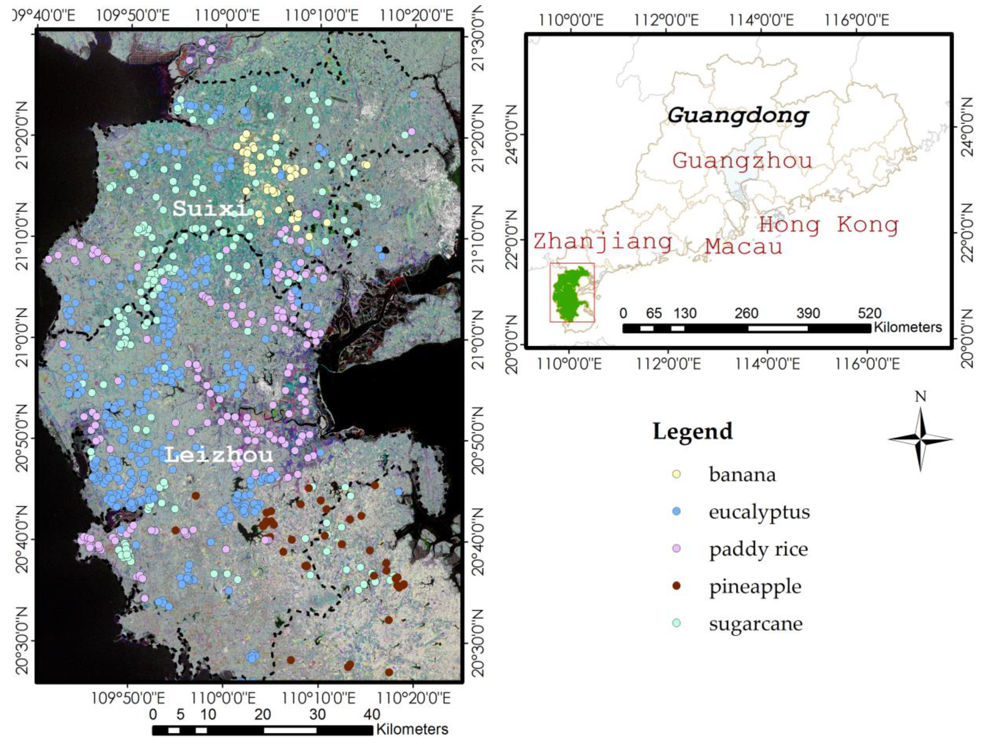
The study area includes Suixi and Leizhou Counties, which are in the southwest section of Guangdong Province, China (
Figure 1). This area has a humid subtropical climate, with short, mild, overcast winters and long, very hot, humid summers. The monthly daily average temperature in January is 16.2 °C (60.6 °F), and in July is 29.1 °C (84.2 °F). Rainfall is the heaviest and most frequent from April to September.
Sugarcane is the most prominent agricultural product of the two counties. Bananas, pineapples, and paddy rice are native products that also play a significant role in the local agricultural economy. In addition, the study area is the most important eucalyptus growing region in China.
2.2. Sugarcane Crop Calendar
As the crop rotates, the growth stages, biomass development, plant morphology, leaf-ground double bounce, soil moisture, irrigation conditions, and surface roughness in the crop field changes, resulting in changes in the backscatter coefficient. The phenological evolution of each crop produces a unique temporal profile of backscattering coefficient. Therefore, the temporal profile in relation to crop phenology serves as key information to distinguish different crop types.
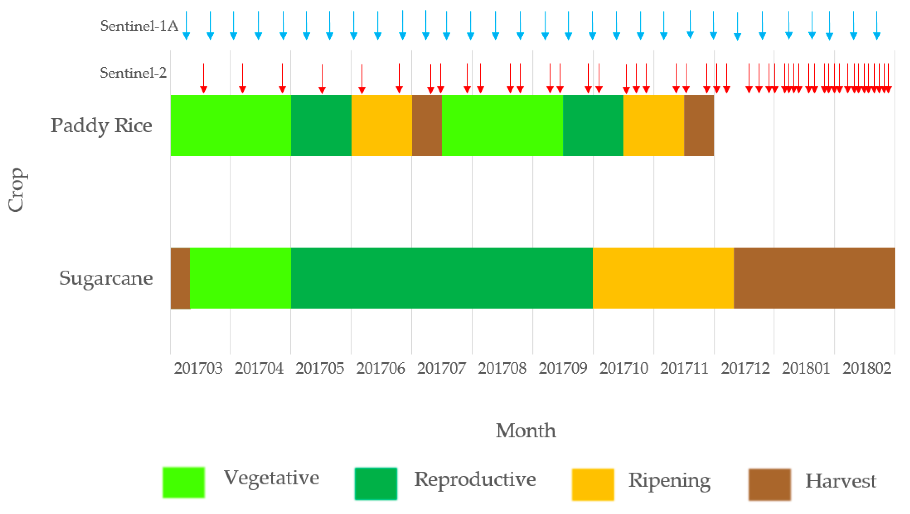
In this study, the phenology of sugarcane and paddy rice in Zhanjiang is categorized into four periods: vegetative, reproductive, ripening, and harvest (
Figure 2). The details of these periods are as follows:
For sugarcane: (1) the vegetative period runs from mid-March through April; (2) the reproductive period lasts from May through September; (3) the ripening period (including sugar accumulation) extends from October to early December; and (4) the harvest begins in late December and lasts until March of the following year (with most sugarcane being reaped in February) [
14].
For first season paddy rice [
22]: (1) the vegetative period (including trans-vegetation) is March and April; (2) the reproductive period is in May; (3) the ripening period is in June; and 4) the harvest begins in July and lasts for 2 weeks. For second season paddy rice: (1) the vegetative period runs from mid-July to early September; (2) the reproductive period lasts from mid-September to early October; (3) the ripening period extends from mid-October to mid-November; and (4) the harvest begins in late November and lasts for 2 weeks.
The banana, pineapple, and eucalyptus growth periods generally lasts 2-4, 1.5-2, and 4-6 years, respectively.
2.3. Sentinel-1A Data, Sentinel-2 Data, and Field Data
For this study, we used the S1A interferometric wide swath GRD product which featured a 12-day revisit time; thus there were 30 imageries acquired from 10 March, 2017 to 21 February, 2018, covering the entire sugarcane growing season. The product was downloaded from the European Space Agency (ESA) Sentinels Scientific Data Hub website (
https://scihub.copernicus.eu/dhus/). The product contains both VH and VV polarizations, which were used to evaluate the sensitivity of each polarization, distinguishing sugarcane from other vegetation.
The S2 data used in this study were the S2A and S2B L1C products. These data provide Top-of-Atmosphere (TOA) reflectance, rectified through radiometric and geometric corrections, including ortho-rectification and spatial registration on a global reference system with sub-pixel accuracy [
37]. The products were downloaded via the S2 repository on the Amazon Simple Storage Service (Amazon S3).
There were a total of 808 sample points (field data) obtained through ground surveys and interpretations in the study area for five main types of local vegetation: eucalyptus, paddy rice, sugarcane, banana, and pineapple. The locations of the points are presented in
Figure 1:
Ground surveys: We specified six major cropping sites based on expert knowledge, then we traveled to each site and recorded raw samples of the crop types at each site and along the way. The recording tools we used were a mobile app and a drone. The app was developed by our team and was used to obtain five corresponding pieces of information, namely, GPS coordinates, digital photos, crop types, photos taken at azimuth, and distances to crop fields. The drone was a DJI Phantom 3 Professional quadcopter (four rotors) and was used to survey the crop fields that were difficult to visit.
Interpretation: the photos taken at azimuth and the distance to crop fields were used to correct the GPS coordinates. Since the app only recorded the coordinates at the cell phone location and most of the crop fields were inaccessible, we needed to correct the coordinates to the centers of the crop fields.
2.4. Sugarcane Mapping Framework
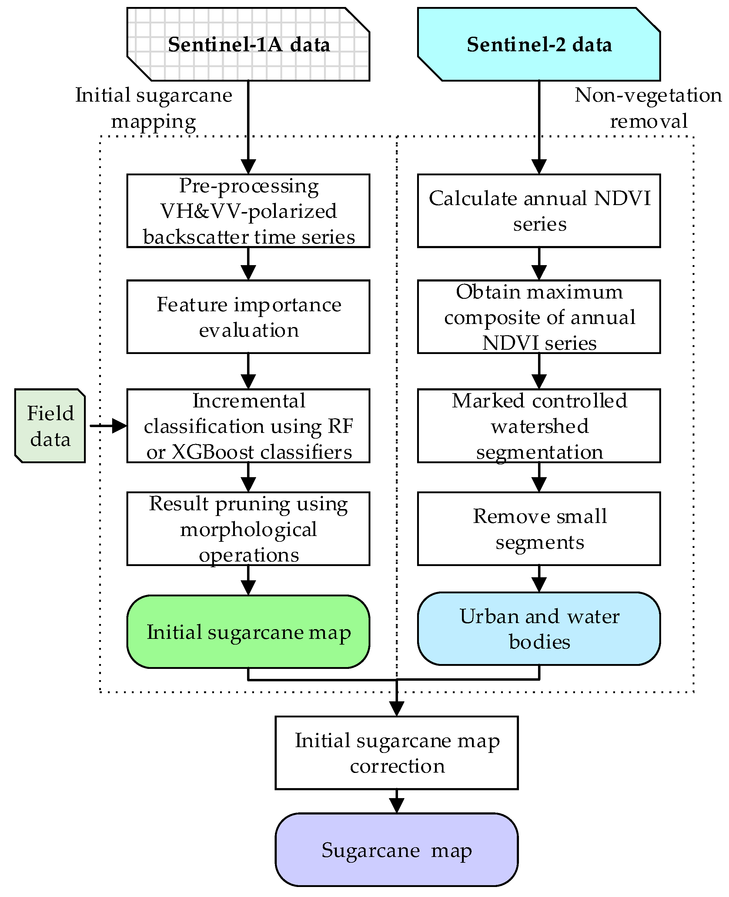
In this study, we proposed a methodological framework for sugarcane mapping using multi-temporal S1A SAR data, S2A and S2B optical data, and field data. The framework was divided into two main processes: initial sugarcane mapping and non-vegetation removal (
Figure 3).
Initial sugarcane mapping: The S1A SAR data for the study area was pre-processed in order to obtain the VH and VV polarized backscatter image time series. Next, to test the performance of the sugarcane early mapping, the image time series were incrementally selected and applied using the RF or XGBoost classifier and a result-pruning method based on morphological operation, which generated an initial sugarcane map.
Non-vegetation removal: Some non-vegetation surfaces included intermittently waterlogged surface which tended to be confused with sugarcane were filed in the S1A data. This study used S2 data to extract the non-vegetation land covers. The Normalized Difference Vegetation Index (NDVI) was first calculated from S2 data. Following that, using annual composites of the maximum filter, the differences between vegetation and non-vegetation were enhanced. Since the non-vegetation surfaces or water bodies are relatively concentrated, we applied marker controlled watershed (MCW) segmentation to the mapping of the non-vegetation surfaces in order to avoid the interference caused by the mixed-pixel effect.
Finally, we employed a non-vegetation mask to correct the initial sugarcane map, thereby producing the final sugarcane map.
The details of the procedural framework are delineated in the following sections.
2.5. Initial Sugarcane Mapping
The Initial sugarcane mapping using S1A SAR data consists of four steps: preprocessing, feature subset selection, random forest classification, and result pruning.
2.5.1. Sentinel-1A Data and Preprocessing
The S1A data were preprocessed using Sentinel Application Platform (SNAP) open source software version 6.0.0. The preprocessing stages included: (1) radiometric calibration that exported image band as sigma naught bands (σ°); (2) ortho-rectification using range Doppler terrain correction with Shuttle Radar Topography Mission Digital Elevation model; (3) reprojection to the Universal Transverse Mercator (UTM) coordinate system Zone 49 North, World Geodetic System (WGS) 84, and resampling to a spatial resolution of 10 m using the bilinear interpolation method [
22]; (4) smoothing of the S1A images by applying the Gamma-MAP (Maximum A Posteriori) speckle filter with a 7 × 7 window size; and (5) transformation of the ortho-rectified σ° band to the backscattering coefficient (dB) band.
2.5.2. Feature Importance Evaluation
Previous studies have shown that SAR images acquired during each phenological period may differ in their sensitivity to crop type. For two periods, one in which crops changes significantly and the other in which the crops are relatively stable, the first would generally contributes more to crop classification. The assumption behind early season sugarcane mapping using the S1A image time series is that the majority of the periods that are sensitive to sugarcane differentiation occur earlier than the insensitive periods. Moreover, the images obtained during the latter phenology stage after sugar accumulation may not be necessary [
14].
To verify this, we first plotted the temporal profiles of each sample type from the S1A image time series in order to visually observe the phenological variation of sugarcane and other vegetation. We then applied the RF and XGBoost classifier to rank the feature importance, respectively. The features used in this study were the 30 images acquired from March 10, 2017 to February 21, 2018. Each image contained both VH and VV polarizations.
The temporal profiles of sugarcane and other vegetation were plotted for both VH and VV polarizations using the preprocessed S1A image time series as well as the training samples mentioned in
Section 2.3. The mean backscatter coefficient was calculated by averaging the sample values for each vegetation type.
The RF classifier proposed by Breiman [
38] is an ensemble classifier that uses a set of decision trees to make a prediction and is designed to effectively handle high data dimensionality. Previous studies in crop mapping have demonstrated that, compared with state of the art classifiers i.e., Support Vector Machines with Gaussian kernel, the RF does not only produce high accuracy, but also features with fast computation and easy parameters tuning [
8,
22]. Several studies have investigated the use of the RF classifier for rice mapping with SAR datasets [
22,
23,
24]. The XGBoost is a scalable and flexible gradient-boosting classification method, which uses more regularized model formalization to control over-fitting, which gives it better performance. In addition, XGBoost supports parallelization of multi-threads while RF does not. Thus it makes XGBoost even faster than RF. Recently, it has been popular in many classification and crop mapping applications [
39,
40,
41,
42,
43]. Considering the intensive computation requirements in sugarcane mapping utilizing different polarizations and random split sample sets, we chose the time efficiency algorithms including RF and XGBoost as classifiers and evaluated their performance.
Both of the RF and XGBoost classifiers have specific hyper-parameters that require tuning for optimal classification accuracy. In this study, a 10-fold cross validation using all samples was performed for both RF and XGBoost classifiers, in order to optimize the key parameters that prevent overfitting (
Table 1). Other parameters were set as default value e.g. parameter “nthread” was set as using the maximum threads available on the system.
In RF and XGBoost classifiers, the relative rank (i.e., depth) of a feature used as a decision node in a tree can be used to assess the relative importance of that feature with respect to the predictability of the target class. Each decision node is a condition of a single feature, designed to split the dataset in two such that similar response values result in the same set. A measure is based on its selection of optimal conditions using Gini impurity. Thus, when training a tree, the amount that each feature decreases the weighted impurity in that tree can be calculated. For a forest, the impurity decrease from each feature can be averaged and normalized, and ultimately used to rank features [
38,
44].
2.5.3. Incremental Classification
In this study, we applied an incremental classification method in order to map sugarcane early in the agricultural season. This method first sets a start time point, then successively performs the supervised classification with the RF and XGBoost algorithm, each time a new S1A image acquisition is available, using all of the previously acquired S1A images [
44]. During this process, each new S1A acquisition triggers three classification scenarios, which are distinguished by the polarization channels used: VH, VV or VH + VV.
The above configurations serve two purposes: one is to analyze the evolution of the mapping accuracy as a function of time, thereby determining the time point at which the sugarcane map reaches an acceptable level of quality; and the other is to determine which polarization (VH, VV or VH + VV) performs best when distinguishing sugarcane from other crops.
2.5.4. Result Pruning
Due to mixed pixel effects, there were many misclassified pixels distributed along the boundaries of crop fields. To remove these errors, we applied a majority filter and two morphological operations, binary closing and binary opening to the initial sugarcane map.
- (1)
Majority filter: Replaces pixels in an image based on the majority of their contiguous neighboring pixels with a size equal to 16. It generalizes and reduces isolated small misclassified pixels.
- (2)
Binary closing: A mathematical morphology operation consisting of a succession of dilation and erosion of the input with a 3 × 3 structuring element. It can be used to fill holes smaller than the structuring element.
- (3)
Binary Opening: Consists of a succession of erosion and dilation with the same structuring element. It can be used to remove connected objects smaller than the structuring element.
Implementation details: The RF classifier used was based on Scikit-learn, version 0.20 [
45]; the XGBoost classifier was based on version 0.82 [
46]; the majority filter was based on GDAL Python script gdal_sieve.py version 2.2.3 and the morphology operations were based on Scikit-image, version 0.14 [
47]. The Python version was 2.7.
2.6. Non-Vegetation Removal
Although non-vegetation elements, including urban land areas and water bodies, were not the focus of this study, they may be confused with various types of crops in S1A VH and VV images. For example, the backscatter coefficients of buildings were high, while the values of cement and asphalt pavements were low. To avoid misclassification, we used the S2 optical data to extract a non-vegetation mask, which was then employed to exclude misclassified crops.
MCW segmentation based non-vegetation extraction, stems from the water extraction method proposed by Hao [
48]. In this study, the non-vegetation surfaces were also used in the MCW segmentation based extraction method but with different input images and parameters.
First, the NDVI (Equation (1)) was calculated from the S2 L1C product; second, a maximum filter was applied to the time series NDVIs in order to generate an annual NDVI composite (Equation (2)), which had the effect of enhancing the differences between vegetation and non-vegetation; third, the highly convincing non-vegetation surfaces and backgrounds were initially labelled using the strict thresholds listed in Equation (3); fourth, by carrying out the MCW segmentations, the remaining unlabeled area were then identified according to the input image gradients between two labelled areas. This method was also implemented using Scikit-image, version 0.14 [
47].
where
and
are the visible red and near-infrared bands in the S2 data, respectively;
is the NDVI time series across 1 year.
Finally, we employed this non-vegetation mask to correct the vegetation map and produce the final map showing sugarcane and other vegetation.
2.7. Accuracy Assessment
The total of 808 sample points was divided into two groups including training and testing samples, which were randomly split and into 485 (60%) and 323 (40%) respectively, of the total sample points for each vegetation type.
The accuracy assessment of the proposed sugarcane method consisted of two steps: (1) construction of the error matrix of sample counts using the confusion matrix; (2) calculation of the overall accuracy (OA), user’s accuracy (UA), producer’s accuracy (PA), and Kappa coefficient of our mapping algorithm based on the error matrix.
Note that in order to reduce the influence of sample split deviation when assessing the proposed method, the random splitting (using the same 60% and 40% proportions) was performed 10 times, which generated 10 sets of training and testing samples.
3. Results
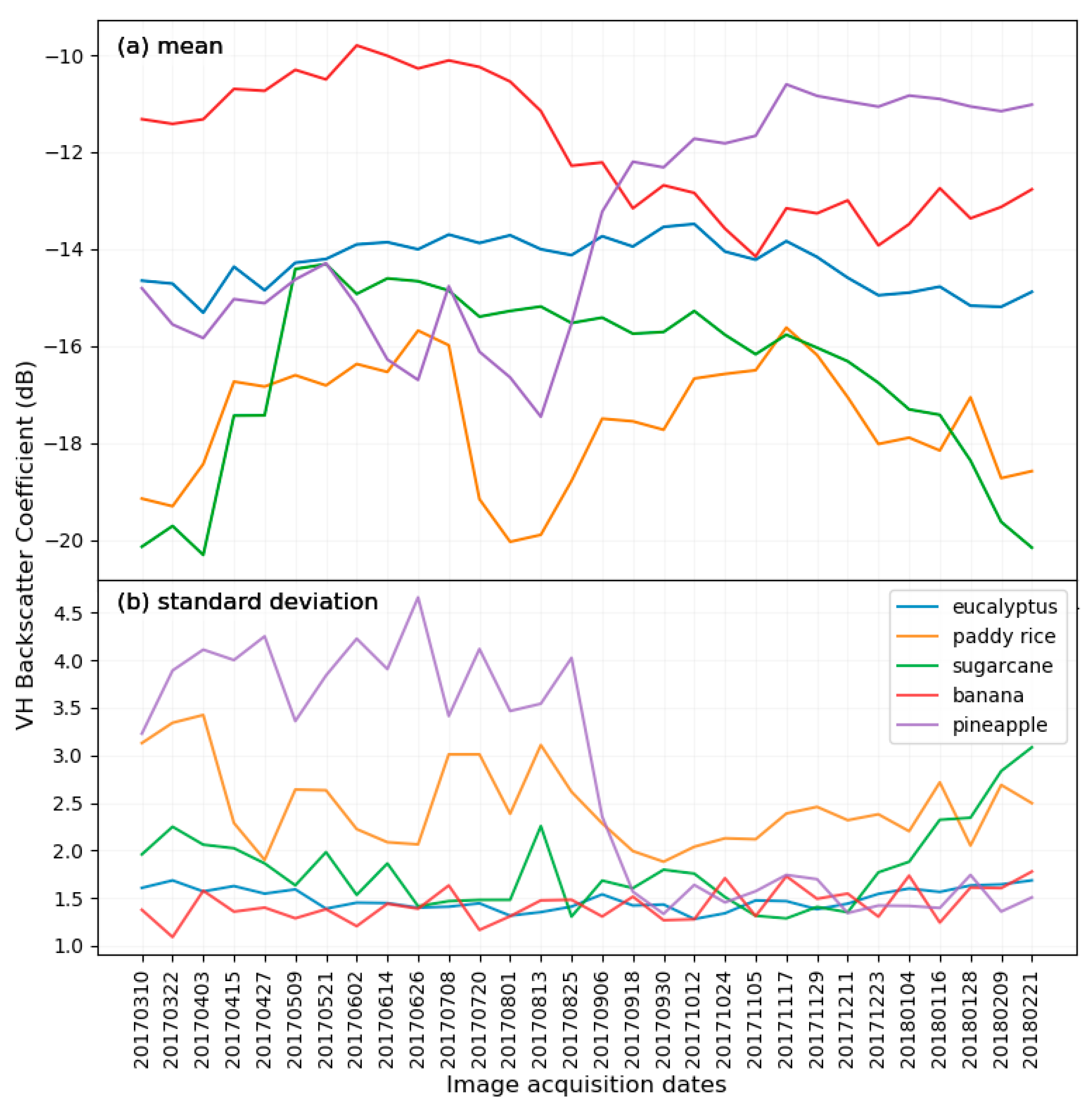
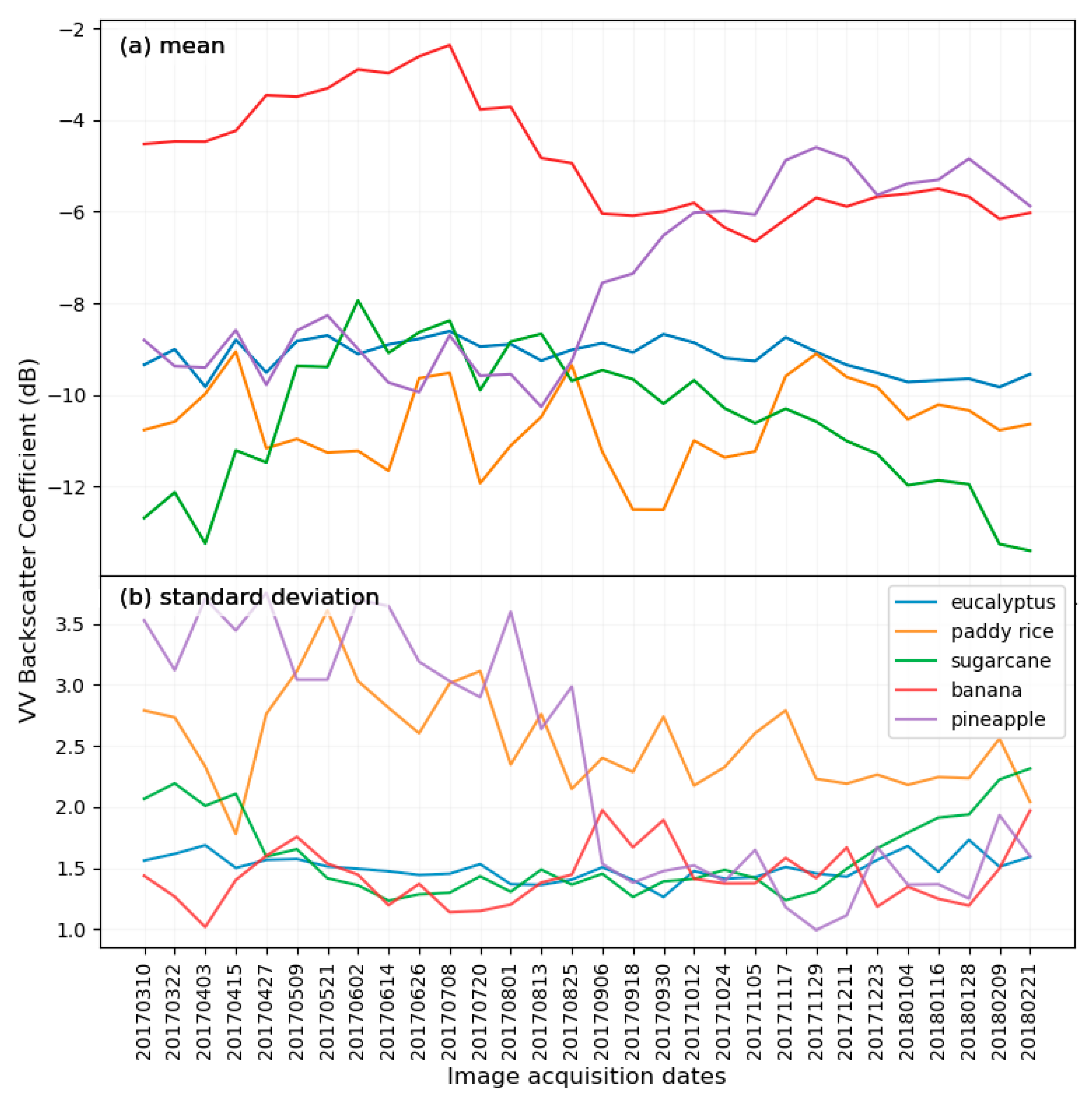
3.1. Temporal Profiles of the Sentinel-1A Backscatter Coefficient
The temporal profiles of sugarcane and other vegetation were plotted for the VH and VV polarizations of the S1A image time series, as shown in
Figure 4 and
Figure 5, respectively.
In general, the temporal profiles of the VH and VV polarizations were similar. Several important characteristics were reflected in both profile types: (1) a sharp increase in the mean of backscatter coefficient from early March to early May, which was during the sugarcane vegetative stage; (2) double-peak characteristics for the two-season paddy rice, which however, was not obvious in the VV profile. This is due to the fact that VV polarization is more sensitive to a waterlogged surface than VH polarization, especially for paddy rice during the reproductive stages [
22]. Despite this, the profile of rice was distinct compared to other crops.; and (3) the profiles of banana, pineapple, and eucalyptus had backscatter coefficients that were larger than those of sugarcane and paddy rice, thereby making the two groups distinct.
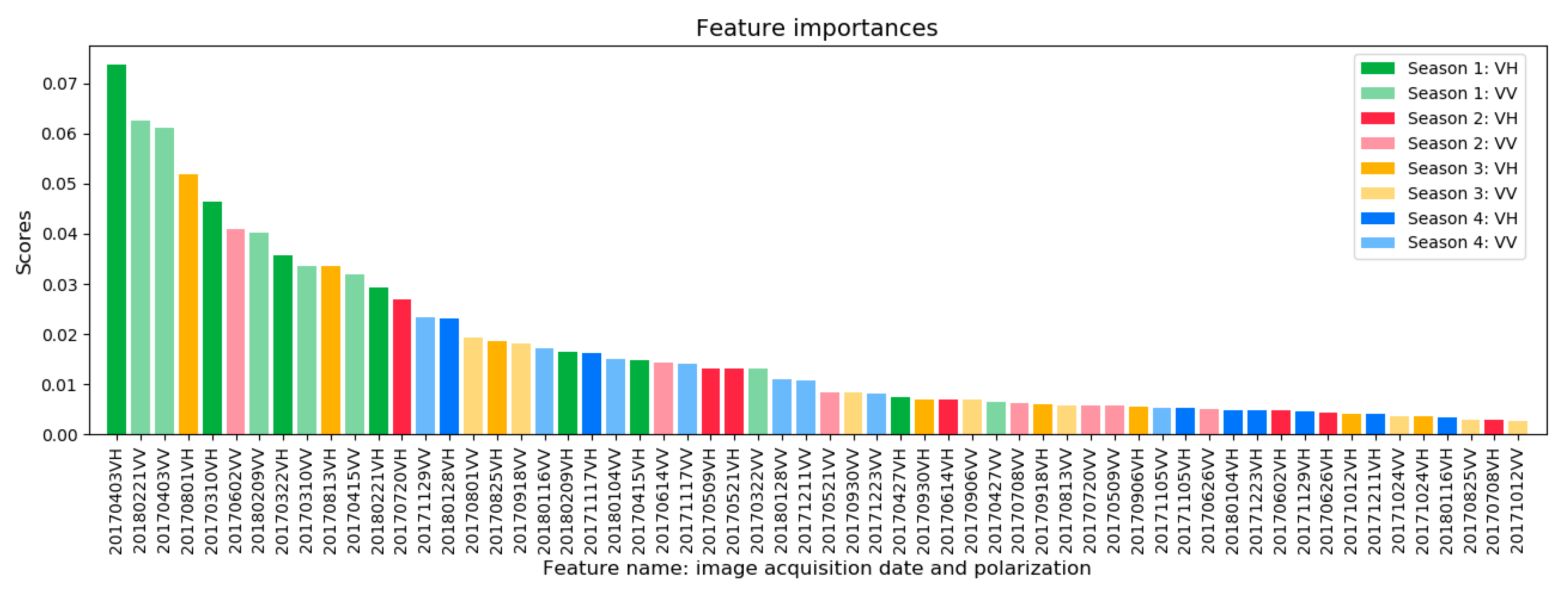
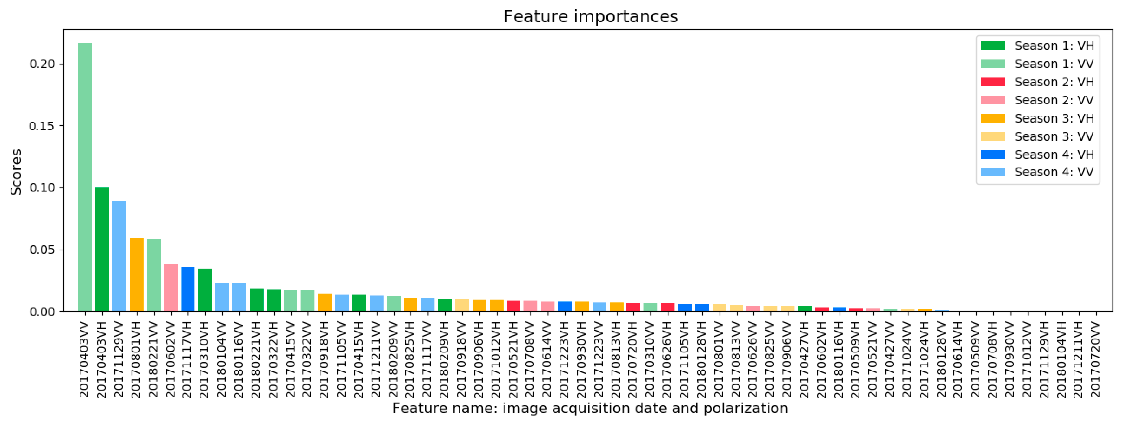
3.2. Feature Importance
The features used in this study were 30 images acquired from 10 March, 2017 to 21 February, 2018. Each image contained both VH and VV polarizations.
Figure 6 and
Figure 7 presents a total of 60 features sorted by decreasing importance in classifying sugarcane and other vegetation. Color coding was used to group features by image acquisition season and polarization: Season 1 from February to April is shown in green, Season 2 from May to June in red, Season 3 from August to October in yellow, and Season 4 for November, December, and January in blue. Both polarizations were plotted using the same color, although the VV polarization bar was set to half-transparent in order to distinguish it from the VH polarization.
The feature importance obtained from RF and XGBoost classifiers are demonstrated in
Figure 6 and
Figure 7 respectively.
In terms of image acquisition dates, Season 1 generally received the highest importance scores, since the vegetative stages of most crops occurred during this time. Although there was a large difference in the orders of feature importance for the two classification methods, images acquired at 10 March, 3 April, 2 June, 1 August in 2017, and 21 February in 2018 appeared among the 10 first features sorted by importance for both methods. Their corresponding phenological stages are listed in
Table 2, these results indicated that this period was critical for sugarcane identification.
In terms of polarizations, although the VV polarization acquired at 3 April, 2017 obtained the highest importance score with XGBoost classifier, in general, there was no significant difference in importance scores for VH and VV polarizations. Therefore, it was difficult to distinguish which polarization was better for sugarcane identification at this step.
3.3. Incremental Classification Accuracy
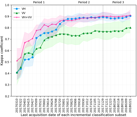
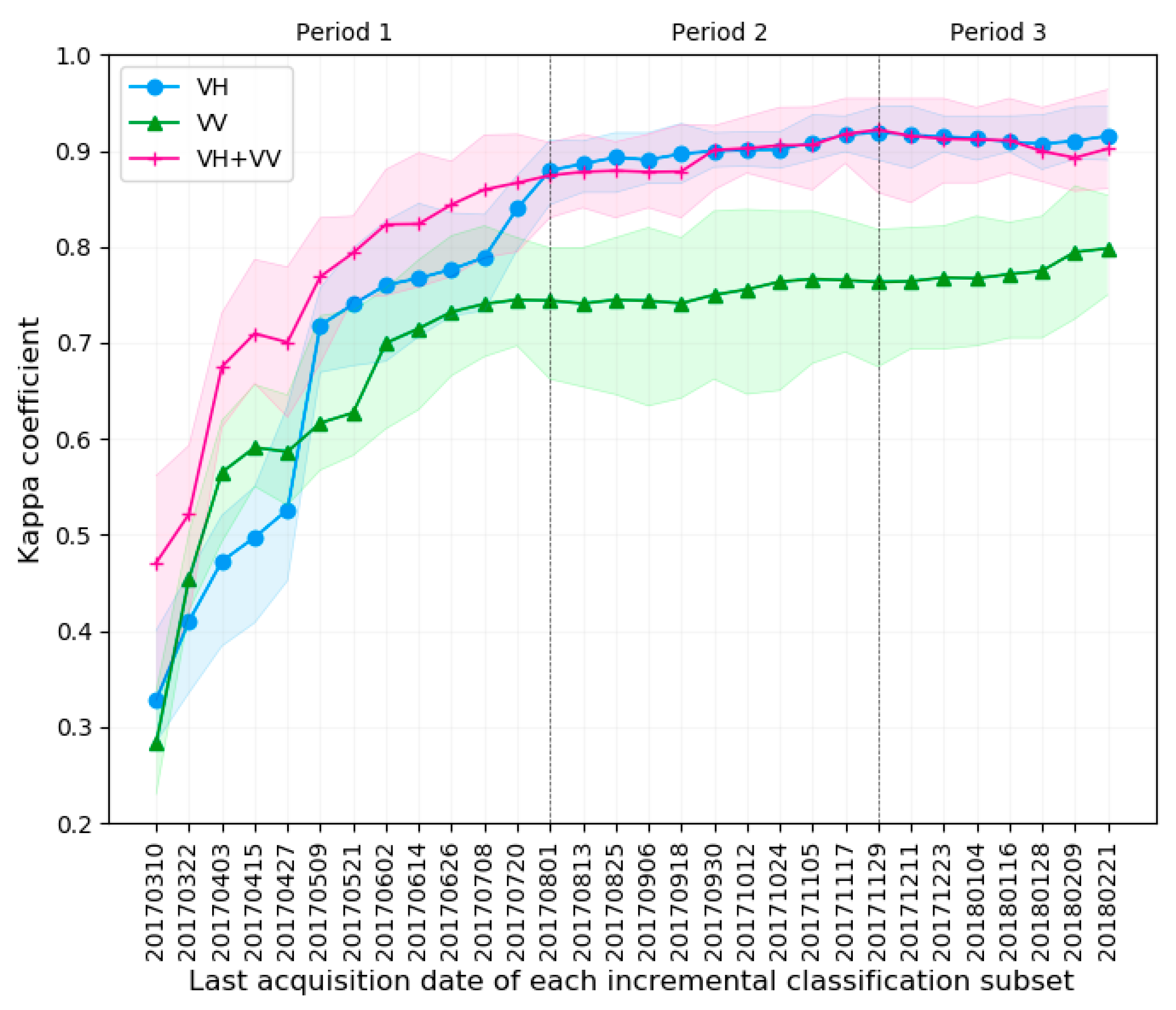
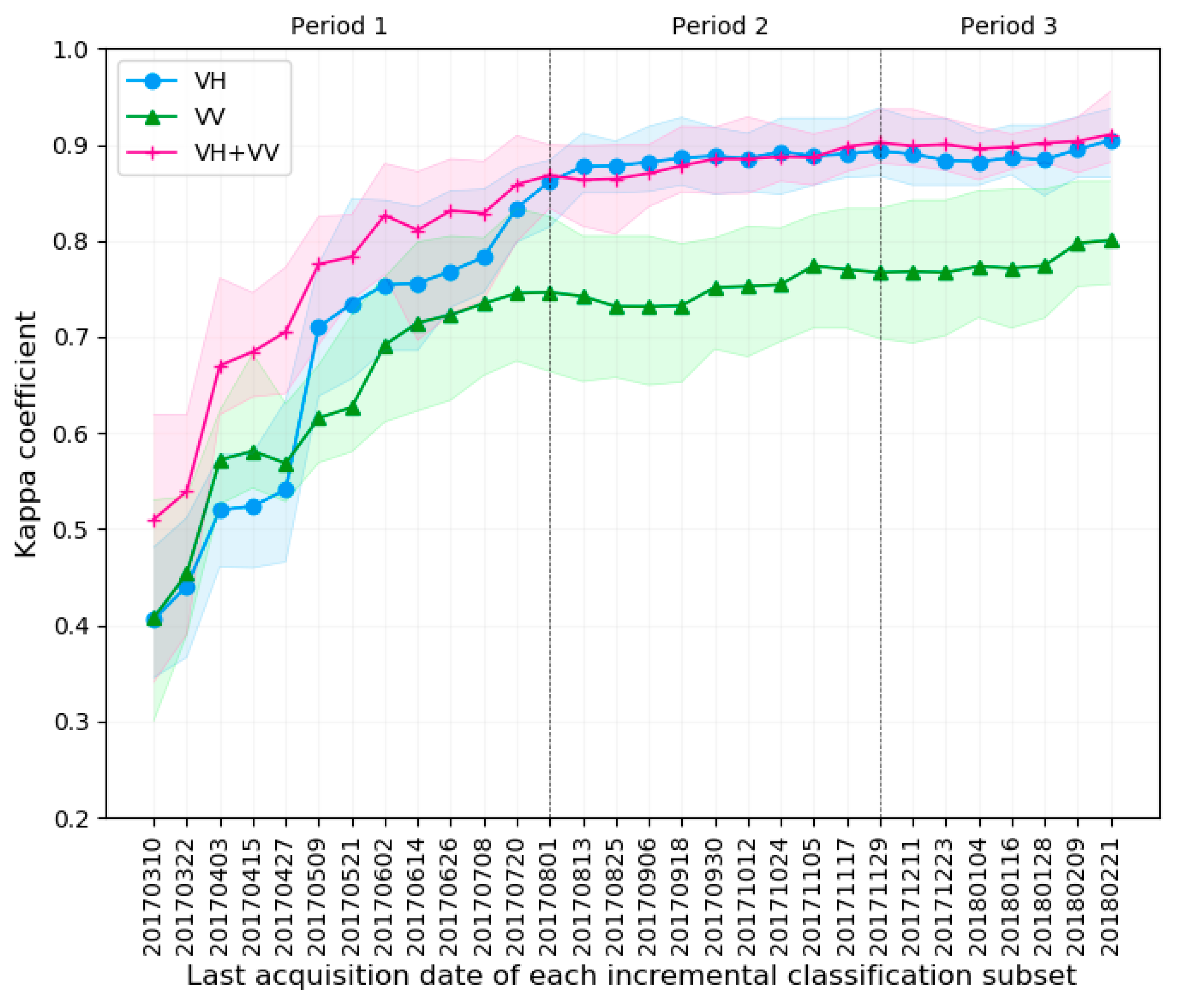
Figure 8 and
Figure 9 summarize the evolution of sugarcane mapping accuracy as a function of image acquisition date using RF and XGBoost classifiers, respectively. At each time point, the sugarcane map was generated and validated 10 times using 10 randomly split sample sets described in
Section 2.7. The mean of accuracy with confidence intervals including maximum and minimum (in terms of Kappa coefficient) are represented by line points, with upper and lower bounds. There were three mapping scenarios: (1) VH polarization alone (blue); (2) VV polarization alone (green); (3) joint VH + VV polarization (red).
In order to clarify the change trend, we used 1 August and 29 November 2017 as the cut-off points and divided the entire time series into the three periods. These two time points were chosen because they corresponded to the end of the harvesting stage of two season paddy rice, respectively.
In period 1, when more data were becoming available as the time progressed, the mapping accuracy of the three scenarios increased rapidly. Among them, the scenario of the joint VH + VV polarization outperformed the other two scenarios. VH polarization alone initially exhibited very low accuracy, however it increased rapidly and caught up with joint VH + VV to a level of 0.880 (RF) and 0.868 (XGBoost) by 1 August, 2017, which was also the time point 7 months before the sugarcane was harvested.
In period 2, the accuracies of the three scenarios increased slowly. Among them, the VH alone and VH + VV scenarios were similar, while the VV scenario exhibited the lowest accuracy. For the RF classifier, the maximum of accuracy using VH and VH + VV scenarios achieved 0.919 and 0.922 respectively and both in 29 November, 2017. At the same time point, using VH and VH + VV scenarios, the XGBoost classifier achieved an extreme accuracy of 0.894 and 0.902 respectively. The time point was three months before the sugarcane was harvested.
In period 3, the accuracy profiles of VH alone and VH + VV exhibited no further improvement for RF but slightly increased for XGBoost, which achieved the maximum accuracy of 0.905 and 0.911 using VH and VH + VV scenarios respectively and both in February 21, 2018.
Despite this, the accuracy profiles were stable in that the variation of accuracy was very small for both classifiers. In addition, the accuracy profile of VV alone showed an increasing trend but was significantly lower than the other two profiles.
Finally, for both RF and XGBoost classifiers, the confidence interval of accuracy yielded by VH + VV and VH scenarios rapidly decreased near 1 August, 2017. In particular, the confidence intervals were larger than 0.11 before this time point and smaller than 0.09 afterwards. The confidence intervals of accuracy yielded by VV scenario were generally large.
3.4. Sugarcane Mapping Results
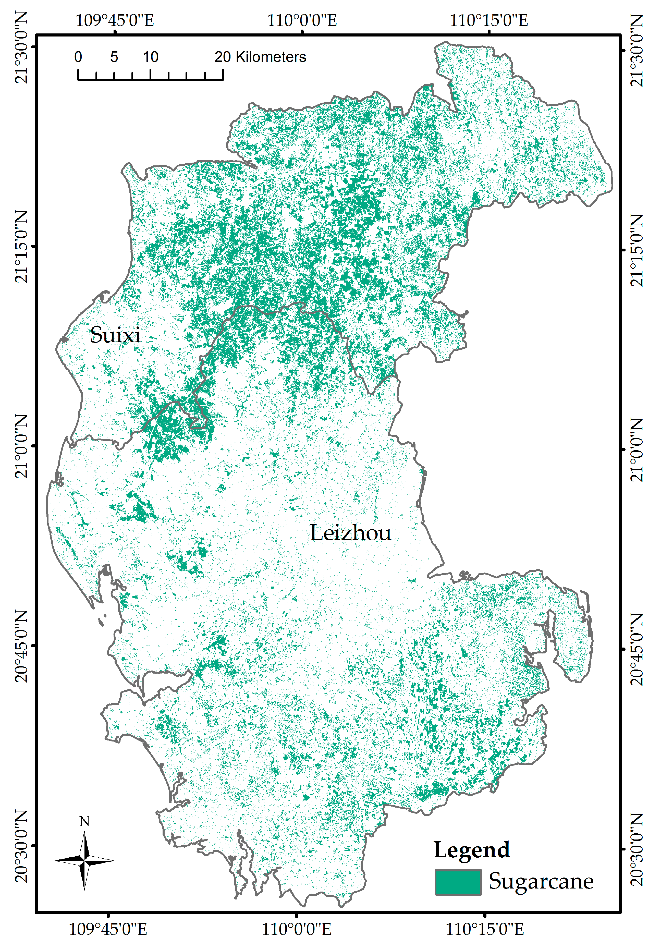
Figure 10 shows the sugarcane extent map generated using the proposed method and the S1A VH + VV imagery time series, ranging from 10 March, 2017 to 29 November, 2017, since our analysis had determined that this data subset was the most accurate.
We tested the proposed method using 323 test points, which represented 40% of the total counts.
Table 3 shows the confusion matrix between the filed samples and the corresponding classification results. The overall accuracy (OA), user’s accuracy (UA), producer’s accuracy (PA), and Kappa coefficients are also displayed. According to
Table 3, the classification determined by this study achieved satisfactory accuracies, with OA of 96% and Kappa of 0.90.
The total sugarcane areas in Suixi and Leizhou for the 2017–2018 harvest year estimated by this study were approximately 598.95 km
2 and 497.65 km
2, respectively. According to the Guangdong RSY in 2017 (the statistics data was for 2016) [
3], the total areas of sugarcane in Suixi and Leizhou were 445.5 km
2 and 518.82 km
2, respectively. Note that the large discrepancy between the sugarcane areas of Leizhou was primarily due to inconsistencies in the sugarcane harvest season and administrative boundaries used by this study and by the RSY. Therefore, we only focus on the relative accuracy of the total sugarcane mapping area, which was approximately 86.3%.
3.5. Computation Speed Comparison
Table 4 shows the time cost of computation (excluding data loading) using two classifiers with 808 samples and full time series, which consisted of S1A image series acquired from 30 imagery acquired from 10 March, 2017 to 21 February, 2018. The tests were performed using a CPU of Intel i7-6700 at 3.40 GHz with 8-cores. Results show the speedup of XGBoost over RF was 7.7, which was roughly equal to the number of threads available.
4. Discussion
In this study, we attempted to develop a method for the early season mapping of sugarcane. First, we proposed a framework consisting of two steps: initial sugarcane mapping using the S1A SAR imagery time series, followed by non-vegetation removal using S2 multispectral imagery. We then tested this framework using an incremental classification strategy with two classifiers, RF and XGBoost.
This method was based on the assumption that the majority of the periods that are sensitive to sugarcane identification occur earlier than those that are insensitive. In order to validate this, we collected 30 S1A imagery acquired from 10 March, 2017 to 21 February, 2018, covering the entire sugarcane growing season. Via feature importance analysis, we discovered that the images acquired from February through April generally received the highest importance scores. This is due to the fact that the vegetative stages of the sugarcane and first-season paddy rice occur during this period.
Incremental classification was performed each time a new S1A image acquisition became available, using all of the previously acquired S1A images. Each new S1A acquisition triggered three classifications with scenarios that included VH alone, VV alone, and joint VH + VV polarizations.
Results indicated that, the maximum accuracy, in terms of Kappa coefficient, achieved by RF classifier using scenarios of VH + VV reached a level of 0.922, which was slightly higher than 0.919 achieved using scenarios of VH alone. However, both the scenarios of VH + VV and VH alone outperformed the scenario of VV alone, which only reached a level of 0.798.
The XGBoost classifier achieved 0.911 using scenarios of VH + VV but were slightly lower than the RF classifier, however it showed promising results: one was that the accuracy profiles and confidence intervals obtained by scenarios of VH + VV and VH alone were similar. This demonstrated that the XGBoost was more robust to overfitting with noisy VV time series than RF; the other was the computing efficiency in that the XGBoost classifier was 7.7 times faster than the RF classifier in an 8-core CPU platform.
As for early season mapping of sugarcane, by using VH + VV polarization, an acceptable accuracy level above 0.902 can be achieved using time series from sugarcane planted up to three months before sugarcane harvest. The accuracy obtained at this period was acceptable, simply because longer time series provided no significant improvements in the sugarcane mapping accuracy.
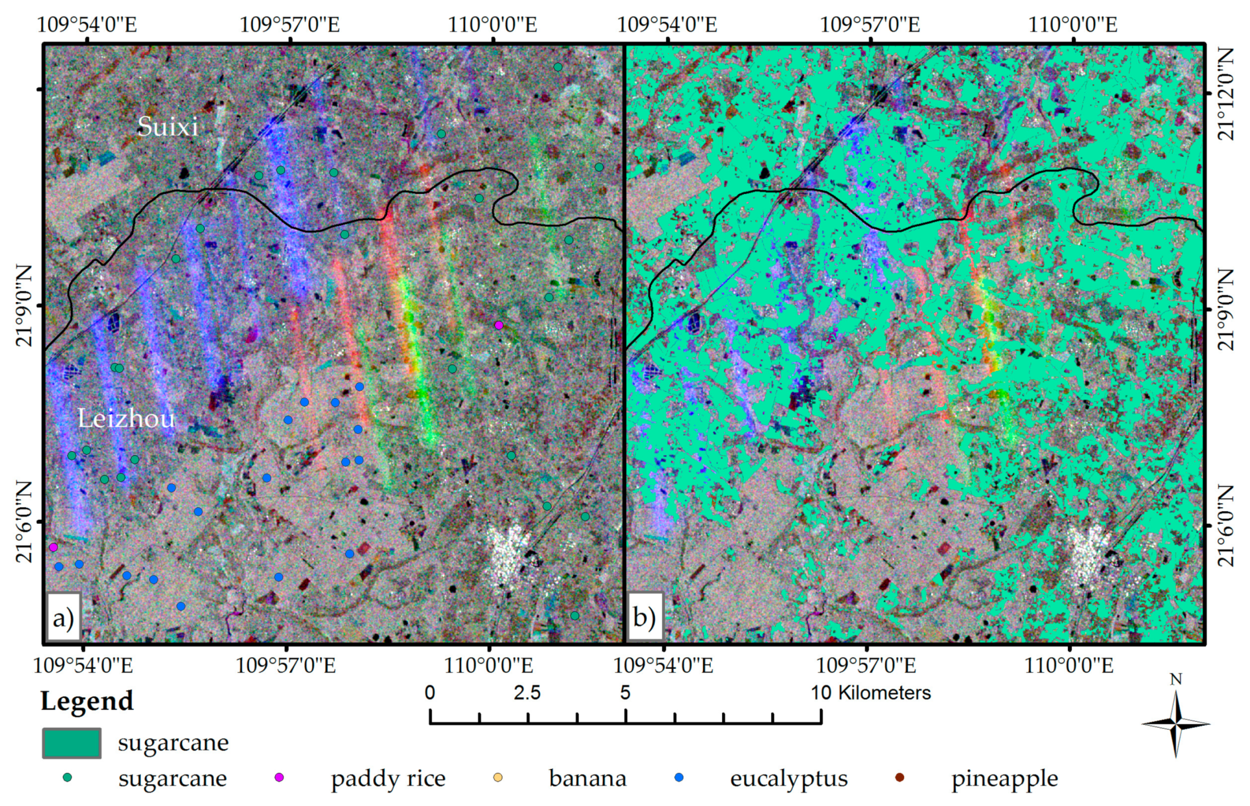
It should be noted that there are two issues related to the accuracy of sugarcane mapping:
First, the initial sugarcane mapping may wrongly identify some non-vegetation pixels including urban area and water bodies. To remove these, we developed two map correction methods: result pruning and non-vegetation removal. However, sample-based validation of the map correction results was difficult to assess, since the artifacts were generally small compared with the urban areas or water bodies. The artifact error should be quantitatively assessed using a map of urban areas and water bodies, something that was beyond the scope of this paper. Considering that these artifacts were located far from the sugarcane fields, their impact on sugarcane mapping accuracy was small. For the sake of brevity, we only presented a single example of result pruning and non-vegetation removal shown in
Figure 11.
Second, there were some white-stripe outliers that featured with very high values in original S1A data, due to electromagnetic interference. These outliers contaminated the observation, making it difficult to recover the original image.
Figure 12 shows an example of 3 S1A VH backscatter coefficients (dB) images in which outliers were concentrated. These images were of northern Leizhou and were acquired on 13 and 25 August and 18 September in 2017. We determined that although the outliers were visually obvious, they did not significantly impact the classification results. This was primarily due to the fact that the probability of outlier occurrence was low. Through visual inspection, we determined that the outliers were randomly distributed spatially and primarily occurred during summer. They appeared at the same position only once or twice throughout the year, whereas there were 30 or 31 images obtained annually. The RF and XGBoost algorithms were robust enough to handle a small number of outliers.
5. Conclusions
In this study, we attempted to develop a method for the early season mapping of sugarcane. First, we proposed a framework consisting of two procedures: initial sugarcane mapping using Sentinel-1A (S1A) synthetic aperture radar imagery time series, followed by non-vegetation removal using Sentinel-2 (S2) optical imagery. Second, we tested the framework using an incremental classification strategy using random forest (RF) and XGBoost classification methods based on S1A imagery covering the entire 2017–2018 sugarcane season.
The study area was in Suixi and Leizhou counties of Zhanjiang city, China. Results indicated that an acceptable accuracy, in terms of Kappa coefficient, can be achieved to a level above 0.902 using time series three months before sugarcane harvest. In general, sugarcane mapping utilizing the combination of VH + VV as well as VH polarization alone outperformed mapping using VV alone. Although the XGBoost classifier with VH + VV polarization achieved a maximum accuracy that was slightly lower than random forest (RF) classifier, the XGBoost showed promising performance in that it was more robust to overfitting with noisy VV time series and the computation speed was 7.7 times faster than RF classifier.
The total sugarcane areas in Suixi and Leizhou for the 2017–2018 harvest year estimated by this study were approximately 598.95 km2 and 497.65 km2, respectively. The relative accuracy of the total sugarcane mapping area was approximately 86.3%.
The effect of non-vegetation removal using S2 NDVI image maximum composites and the influence of outliers caused by electromagnetic interference on sugarcane mapping were also discussed.
Future work intends to incorporate non-vegetation removal with a road identifications method thus further improving the accuracy of sugarcane mapping. In addition, we are going to apply the proposed method on the mapping of major crops in Guangdong province, China.

 ,
, 


