Use of WorldView-2 Along-Track Stereo Imagery to Probe a Baltic Sea Algal Spiral

Remote Sensing Division, Naval Research Laboratory, Washington, DC 20375, USA
*
Author to whom correspondence should be addressed.
Remote Sens. 2019, 11(7), 865; https://0-doi-org.brum.beds.ac.uk/10.3390/rs11070865
Submission received: 26 March 2019
/
Revised: 5 April 2019
/
Accepted: 8 April 2019
/
Published: 10 April 2019
(This article belongs to the Special Issue Very High Resolution (VHR) Satellite Imagery: Processing and Applications)
Abstract
:The general topic here is the application of very high-resolution satellite imagery to the study of ocean phenomena having horizontal spatial scales of the order of 1 kilometer, which is the realm of the ocean submesoscale. The focus of the present study is the use of WorldView-2 along-track stereo imagery to probe a submesoscale feature in the Baltic Sea that consists of an apparent inward spiraling of surface aggregations of algae. In this case, a single pair of images is analyzed using an optical-flow velocity algorithm. Because such image data generally have a much lower dynamic range than in land applications, the impact of residual instrument noise (e.g., data striping) is more severe and requires attention; we use a simple scheme to reduce the impact of such noise. The results show that the spiral feature has at its core a cyclonic vortex, about 1 km in radius and having a vertical vorticity of about three times the Coriolis frequency. Analysis also reveals that an individual algal aggregation corresponds to a velocity front having both horizontal shear and convergence, while wind-accelerated clumps of surface algae can introduce fine-scale signatures into the velocity field. Overall, the analysis supports the interpretation of algal spirals as evidence of a submesoscale eddy and of algal aggregations as indicating areas of surface convergence.
1. Introduction
High spatial resolution imagery from satellites capable of along-track stereo, or from satellites that follow each other closely in time on similar orbits, can be exploited for target motion given appropriate time lags between the image acquisitions [1,2,3,4,5,6,7,8,9]. In the ocean, targets take the form of spatial gradients and other features in ocean color and surface temperature, suspended material, surface films, and (as in this work) algae. Ocean currents can be deduced from time-lagged images by using various techniques such as maximum cross-correlation [2,4,8] and optical flow [4,5,6,7,8,9]. Particularly exciting is the possibility of using high-resolution time-lagged imagery to explore the realm of the ocean submesoscale, in which strong surface convergences and downwelling become associated with horizontal density fronts and cyclonic vortices e.g., References [10,11].
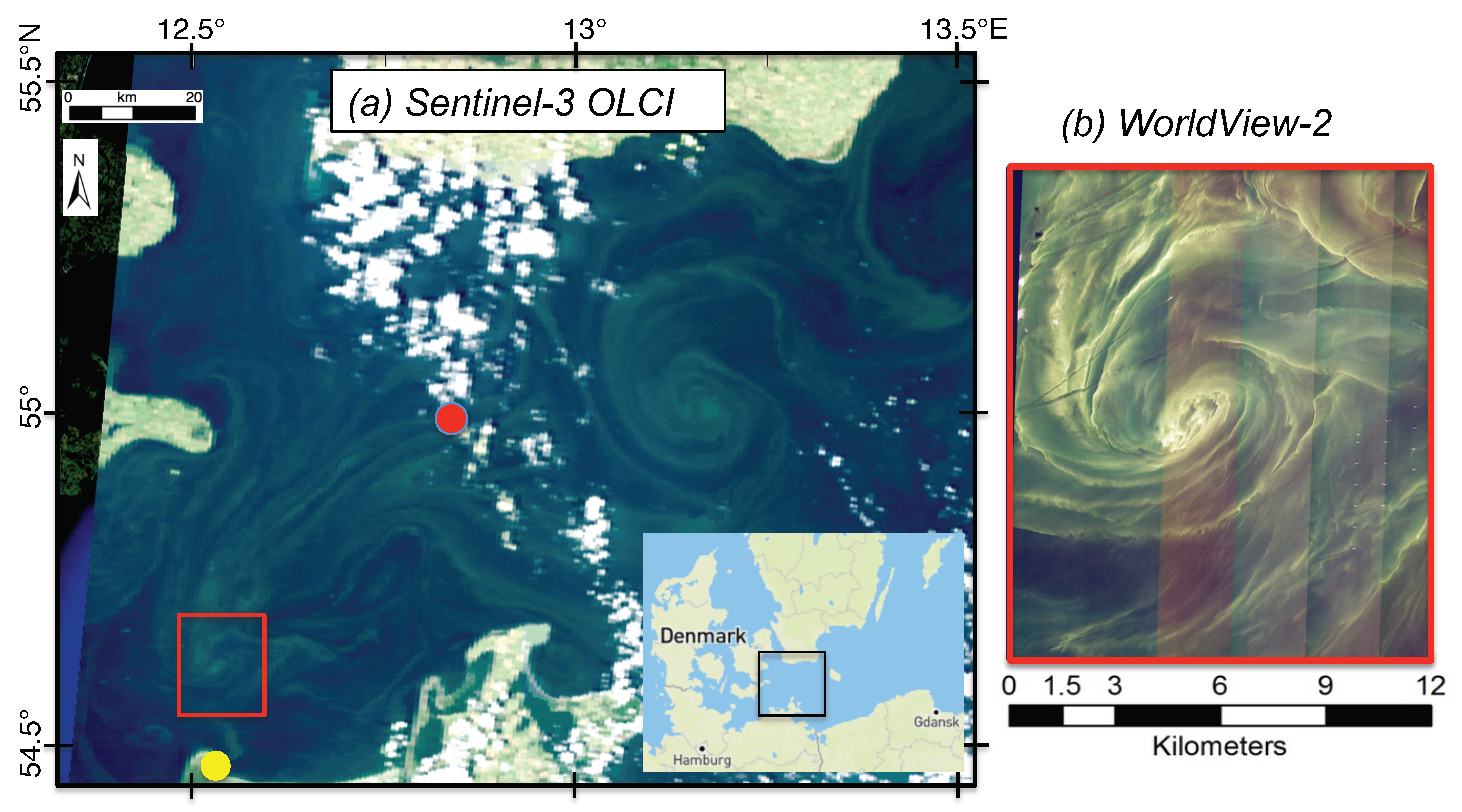
In this letter, a single pair of along-track stereo images from the WorldView-2 satellite (DigitalGlobe, Inc., Westminster, CO, USA; pixel sizes of ~1 m) is used to examine aspects of small-scale dynamical features as revealed through an algal bloom in the western Baltic Sea. A large-scale view of the study area is provided by a Sentinel-3 satellite image (Figure 1a). The numerous green filaments and spiral patterns in the imagery are caused by buoyant cyanobacteria (blue-green algae), which commonly form summer blooms, often toxic, on the surface of the Baltic Sea under relatively low wind conditions [12,13]. An understanding of and an ability to predict concentrations of cyanobacteria are of practical importance and interdisciplinary interest. The WorldView imagery captures a small algal spiral pattern (Figure 1b) that provides the focus of this study. High-resolution stereo views of submesoscale phenomena are rare in the Baltic Sea and other areas as well; and in the present case, may provide insight into how the various algal patterns arise and what might be learned from them. For instance, the relationship of the spiral pattern to ocean dynamics remains unclear. It is reasonable to suppose that a spiral pattern derives from the action of an underlying eddy, but to our knowledge this has never been confirmed directly. Assuming an eddy, then how does the spiral pattern arise? Is it from kinematic distortion (i.e., from a differential angular velocity of the fluid) of any initial distribution of algae material [14], or is it from the dynamics of the fluid, in which the cyanobacteria, like any other surface floating material, become concentrated along frontal convergence zones that are being swept into the eddy [10]?
In order to address such questions, the WorldView stereo data are analyzed here using an optical-flow algorithm to deduce the velocity field. There are, however, a variety of noise sources— such as signal processing, data collection configuration, and environmental factors—that can contaminate the results. A scheme for ameliorating the effect of one processing artifact (“striping”) is described and used in this work. As will be shown, the analysis does indeed reveal a vortex at the center of the algal spiral, which supports the interpretation of such algal spirals as evidence of a submesoscale eddy, and that an individual algal aggregation corresponds to a velocity front having both horizontal shear and convergence (and hence, downward transport).
2. Materials and Methods
2.1. Dataset
The WorldView-2 data were acquired on 1 July 2018, at 10:14:35 UTC (time t1; shown in Figure 1b) and 10:15:52 UTC (time t2); the time interval between data collections being Δt = t2 − t1 = 77 s. While only a segment of the imagery is examined in this study, browser versions of the full image strips can be accessed at https://discover.digitalglobe.com/; select “Area of Interest”; then “Search by image ID”, where the identification numbers for the t1 and t2 images are 10300100803F8400 and 10300100819E2800. The t1 and t2 collections had similar off-nadir angles (25° and 31°), but necessarily different target azimuth angles (261° and 333°). Solar elevation and azimuth angles were 57° and 155°. After geo-referencing and resampling to a uniform UTM map grid, spatial resolution is Δx = 2 m for the eight color and near-infrared bands and Δx = 0.5 m for the panchromatic band. A further step of image-to-image registration using a simple translation and ground control points, results in rms displacement errors of about 1 pixel. High spatial resolution combined with relatively large image time difference yields a velocity detection threshold Δx/Δt of 0.01 to 0.03 m s−1.
Wind data are available from the German research platform FINO-2 (55.007°N, 13.154°E), and a close-by land station (54.443°N, 12.558°E). (See Figure 1a for locations; see Figure S1 for time series). During the 48-h period prior to acquisition of the WorldView imagery, the mean 10-m wind speed at FINO-2 was 3.3 m s−1 (s.d. = 1.3 m s−1). For the hour immediately preceding image acquisition, the mean wind speed was 4.2 m s−1 at FINO-2 and 2.2 m s−1 at the land station, and the mean wind directions were 41.1° and 22.5°. In-water temperature and salinity measurements are also available from FINO-2, and profile and time series plots are shown in Figures S2 and S3. Stratification is dominated by temperature; the water column is weakly stratified in the upper 10 m, and becomes increasingly stratified toward the bottom. The stratification changes little over time, suggesting that horizontal spatial gradients are relatively weak.
2.2. Selection of Wavelength Bands to Analyze
An optimal signal would have a large dynamic range or image contrast and it would represent radiation backscattered from features at the sea surface, so that the derived velocity field could be ascribed to a fixed depth. The latter is an issue because the algae, in addition to forming accumulations at or very near the sea surface, will be dispersed by wind-induced shear and Langmuir circulation, and thus will have some vertical distribution. A dynamic range for an individual wavelength band can be defined as the rms signal in areas having real ocean structure minus that in areas where the signal is near the noise level. Values for the various WorldView bands were thus found to be as follows: highest (6.1 and 5.3 counts) for green and yellow wavelengths (bands 3 and 4); lowest (0.5 to 1.5 counts) for the shortest and the near-infrared wavelengths (bands 1, 2, 7, and 8); and intermediate (about 3 counts) for the red and red-edge wavelengths (bands 5 and 6). As the green wavelength band (band 3; 510 to 580 nm) had the best dynamic range, it was chosen for analysis. A segment of panchromatic data (dynamic range of 5.8 counts) will also be examined; although those data overall have a large percentage of signal near near-noise level, they do capture the finest-scale variations in the algal distributions.
As to the issue of what depth to associate with the derived velocity field, we can note that algal features were found to be highly coherent across bands 3 through 6. Band 6 (wavelengths of 706 to 746 nm) has a penetration depth of 0.75 m, based on the inverse attenuation coefficient for pure water; in the midst of an algal bloom, that depth is likely less. This suggests that, even though the algae may be mixed vertically downward several meters (see Section 3.2), the backscattered signal will be weighted toward the upper meter or so; hence, we assume the velocity field derived using band 3 represents the flow over the upper 1 to 2 meters of the water column.
2.3. Treatment of Noise Stripes
A push-broom instrument such as WorldView-2 uses a linear array of detectors arranged perpendicular to the flight direction of the spacecraft; different areas of the Earth’s surface are then imaged as the spacecraft flies forward. As different electronic amplifiers are used to process sequential sub-arrays of detector elements, small residual errors inevitably arise across the array [15]. Such errors give rise to a pattern of prominent vertical stripes in imagery having a small dynamic range, which is often the case for imagery of the ocean. Such stripes are clearly visible, for example, in Figure 1b, which combines data from red, green, and blue wavelengths (bands 5, 3, and 2, respectively). Striping occurs in every wavelength band, including the panchromatic band, but to a varying degree; and, after geo-referencing data from any wavelength band, a particular stripe will appear in a different geographic location in the t1 and t2 images. The stripe—particularly the abrupt transition, or a jump from one stripe to another—can then be falsely interpreted as an ocean feature that has moved, and this will introduce noise into an image-derived velocity field. An initial de-striping of the data is thus an important step.
Approaches described in the literature [16,17] are based on deriving a polynomial to describe the detector variations across the entire image; this typically results in different corrective adjustments or offsets for every pixel across the push broom. Our approach differs in that it attempts to correct for only the effects of the most significant jumps, which often are regularly spaced across the image and readily identified. The approach consists of the following steps, all of which are done prior to geo-referencing the image data. First (step 1), the position of each jump and its height are determined through examination of an otherwise locally homogeneous part of the image. Second (step 2), the heights are applied uniformly and cumulatively within each stripe to create a one-dimensional array or row of offset values. (A minor complication arises because of a small overlap in the sub-array processing; as a consequence, a jump from one stripe to the next occurs over a range of pixels—about 7 pixels in this dataset.) Lastly (step 3), the offsets are used to de-stripe the data image.
We found it convenient to do both steps 1 and 3 within the image-processing environment of ImageJ [18]. For step 1, we use the ImageJ “Plot Profile” tool in areas of the image where the real ocean signal variation is weak compared to the jump. (To increase the precision to which the jump heights are determined, all data values are first multiplied by one hundred.) For step 3, the imported row of offsets is replicated sufficiently to make an image of the same size as the data image, and is then subtracted from it using ImageJ’s “Image Calculator”. Figure S4 shows the data both before and after the de-striping.
2.4. Method for Calculating Currents
Optical-flow methods estimate the velocity field by assuming conservation of a passive tracer; i.e., the total (Lagrangian) derivative of the tracer is equal to zero for a suitably short time interval. This condition is represented as an exact integral of the nonlinear tracer-conservation equation
where I is tracer intensity, ∆t is the time difference between the two images, and r and u are the position and velocity vectors for a particular image pixel. For the present application, we use a nonlinear optical-flow method called the Global Optimal Solution [5,6,7]. In this approach, the image is partitioned into a number of square sub-domains (called tiles), n pixels on a side. The velocity field within each tile is modeled by a bilinear function. Velocity vectors at the tile nodes are derived through minimizing a cost function that is the sum of errors arising from the use of equation (1) at every pixel; an iterative technique is used that employs Gauss-Newton and Levenberg-Marquardt methods. Choice of tile size depends on the correlation length scale and noise level of the image data [7]. Our procedure at present is to try a range of tile sizes, then choose the one that is small enough to capture the features of interest without excessive noise. In this study, a value of n = 300 pixels with the band-3 data yielded a satisfactory result (see later Section 3.1); a value of n = 50 pixels was used with the panchromatic data.
I(r + u ∆t, t2) = I(r, t1)
A problem with any optical-flow method as applied to ocean imagery is sensitivity to intensity value changes that do not result from local surface currents; this is always a potential source of noise in the calculation [4]. An example would be changes in reflectance as the result of changes in viewing angles; another is contamination by non-ocean features such as clouds. To help mitigate such problems, two pre-processing steps are taken. The first is normalizing the images to have the same overall standard deviation and mean intensity levels. The second is creation of an image mask. In the present case, the elements of the mask include small clouds (and their shadows) that occur in the northwest corner of the image scene, an aircraft in the center-left part of the t2 image, and an underway boat near the top edge. The mask of that boat includes the part of the boat’s turbulent wake that formed between the t1 and t2 views, as this is a case where the tracer (the wake segment) is clearly not conserved between the two images. We did not, however, mask boat-generated internal waves that extend across the upper-middle part of the scene. (These are visible probably because of variations in reflected sky radiation resulting from internal wave-induced modulation of sea-surface roughness.) As internal waves propagate relative to the ambient fluid, they may contaminate estimates of the ambient water velocity.
After computing the velocity field, the vertical component of vorticity and horizontal divergence are calculated. These have their usual definitions: vorticity ζ = ∂v/∂x − ∂u/∂y, and horizontal divergence δ = ∂u/∂x + ∂v/∂y, where (u, v) are the (x, y) components of horizontal flow.
3. Results
3.1. Spiral Pattern (Band 3 Data)
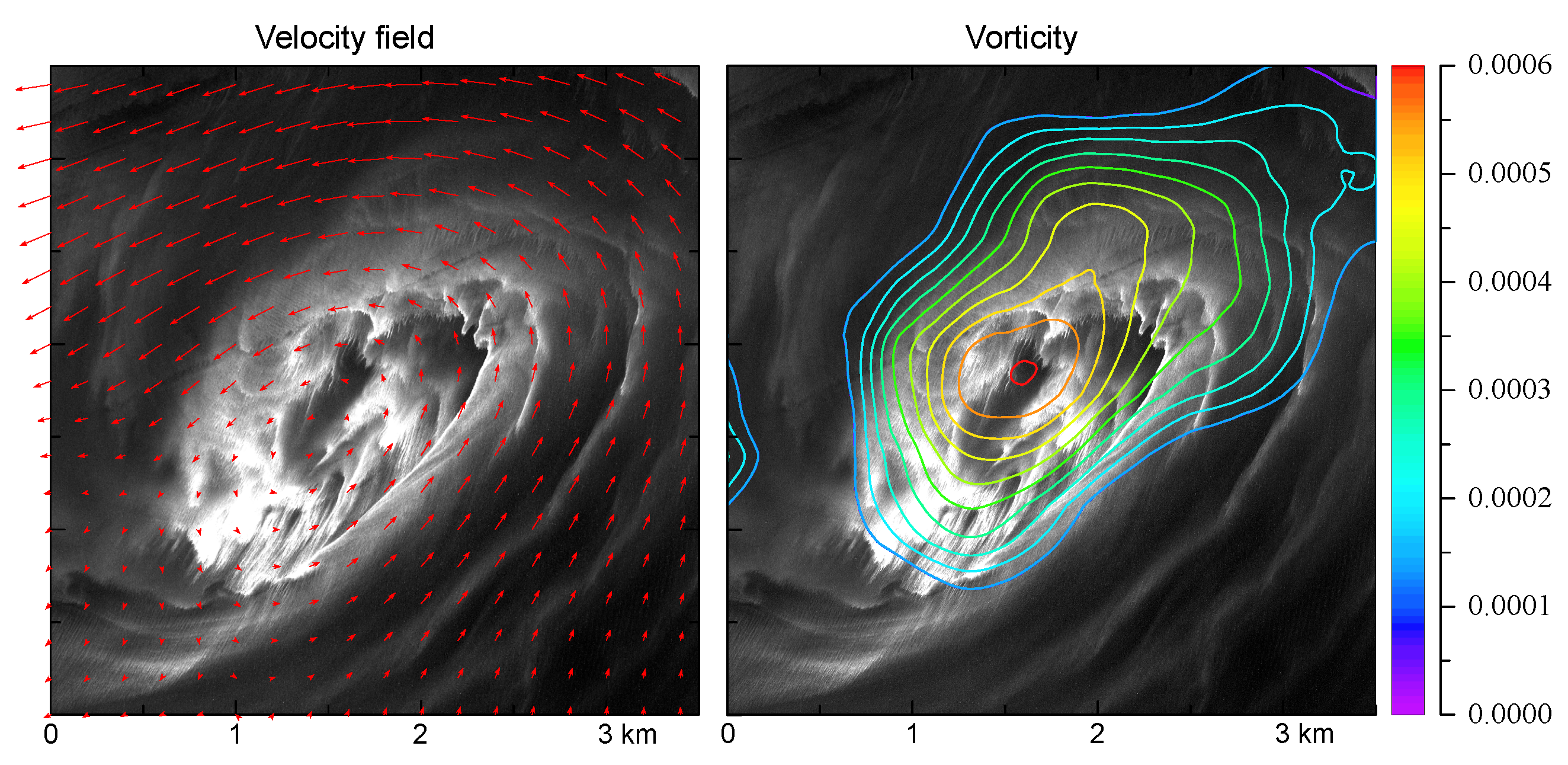
Results from analysis of the spiral pattern using band 3 data are shown in Figure 2. To help distinguish any circulation pattern associated with the spiral, the velocity field (Figure 2a) was computed after first spatially translating the t2 image to compensate for a 17-m southwestward drift of the spiral pattern between the t1 and t2 views. The dominant feature in the velocity field is an area of cyclonic (counter-clockwise) swirling flow that overlies what seems to be, based on the algae pattern, the visual center of the spiral pattern. This oval-shaped vortex is the central feature in the vorticity field (Figure 2b), though other features occur that may not all represent real dynamical features of the flow; see next section. In order to derive some properties of the vortex, we chose a contour level of 2.2 × 10⁻⁴ s−1 (e−1 times the maximum vorticity) to delineate a core region of the vortex. The objective here is to capture as much of the core vorticity as possible without including a possible errant signal, as represented by the lower-level contours that deviate from the overall oval shape. The area of the core was then used to estimate an approximate radius R = 1.1 km, and a mean vorticity ζcore= 3.8 × 10⁻⁴ s−1 (s.d.=1.0 × 10⁻⁴ s−1); equivalently, ζcore = 3.2 f, where f = 1.19 × 10⁻⁴ s−1 is the local Coriolis frequency. As could be expected, the core radius and vorticity do vary with computational scale (i.e., tile size n): At lower resolution (n = 400), the radius is larger (1.37 km) and mean vorticity smaller (2.7 × 10⁻⁴ s−1); at higher resolution (n = 200), the radius is smaller (0.91 km) and mean vorticity larger (4.1 × 10⁻⁴ s−1). The divergence field (not shown), when averaged over the core area, yields values not significantly different from the background.
The character of the vortex core is of course just a part of a description of the eddy’s hydrodynamics, as the spiraling arms of cyanobacteria accumulations extend over a much larger area. In synthetic aperture radar (SAR) imagery, at wind speeds of 0.2 to 5.6 m s−1, the spiral arms would appear as relative dark streaks because of the wave-damping effect of algae-derived surface films. Sub-mesoscale eddies are thus manifested in SAR imagery as “black” spirals [19]. In the Baltic Sea, such black eddies have a mean diameter D = 6.4 km (s.d. = 4.0 km) [20], where D is measured between the most remote edges of the spiral pattern. One way spiral eddies can form is through ageostrophic baroclinic instability associated with a background horizontal density gradient; and theoretical studies [21] show such eddies to have cyclonic vorticity and a spiral diameter D = 2 Rd, where Rd = (g Δρ/ρ H) 1/2 / f is the baroclinic deformation radius. Analysis of SAR spirals in the Baltic, Black, and Caspian seas shows that nearly all the spirals have a morphology consistent with cyclonic vorticity [19,20], a diameter proportional to Rd [20], and are statistically associated with lateral density gradients [20]. Our analysis explicitly reveals the cyclonic vorticity, and based on the available measurements of water stratification, we estimate a value of Rd ~ 3.7 km, which is close to a climatological value of 3.9 km near the study site [22]. These values of Rd can be compared with D/2 ~ 3 km, where D ~ 6 km is the distance between the farthest spiral arms in Figure 2. Our estimate of ~1.1 km for the radius of the vortex core is smaller than both D/2 and Rd, thus making the vortex itself a submesoscale feature. Other studies [10,23] support the notion of a relatively small submesoscale vortex core and convergence bands at larger radius that spiral inwards toward the core.
3.2. Algal Aggregations (Panchromatic Data)
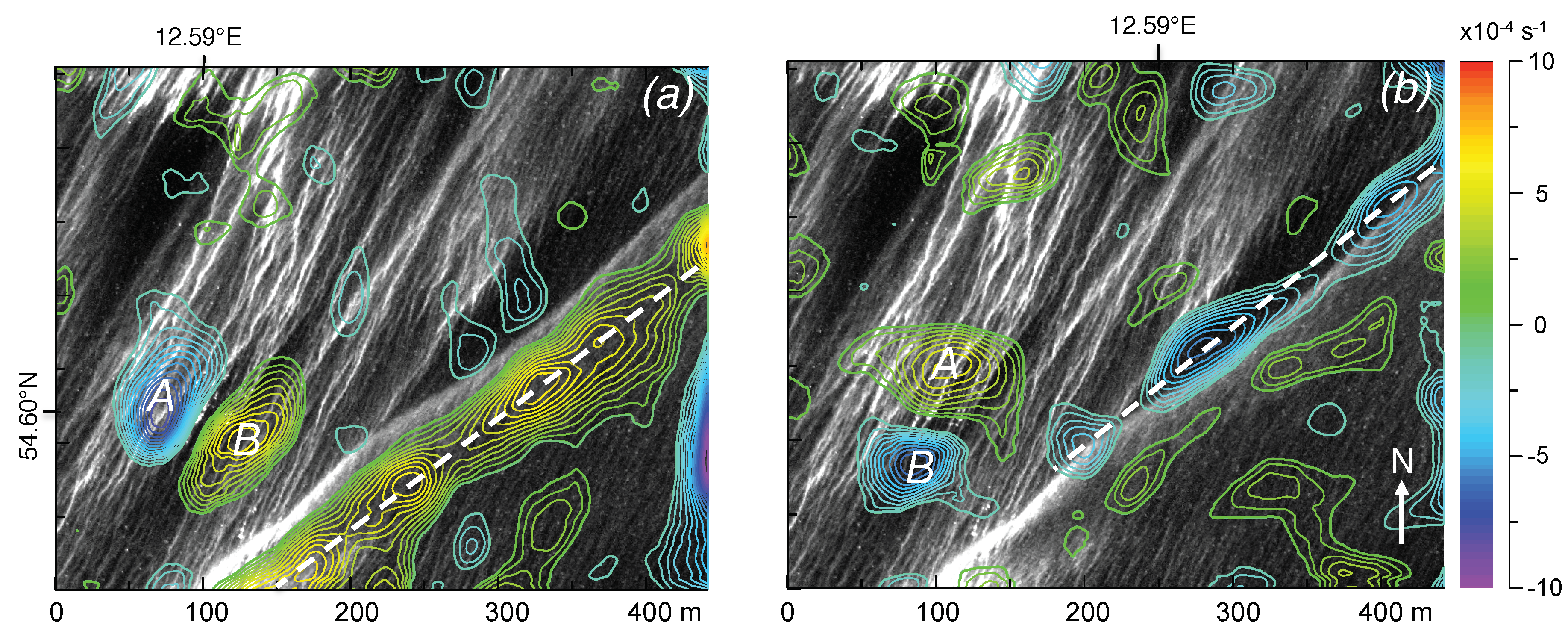
As an example of panchromatic data, we zoom into a representative area (Figure 3) within the spiral that shows two classes of algal features: windrows (the numerous bright streaks) and a long, individual algal aggregation that extends from the x axis toward the northeast, which we examine first.
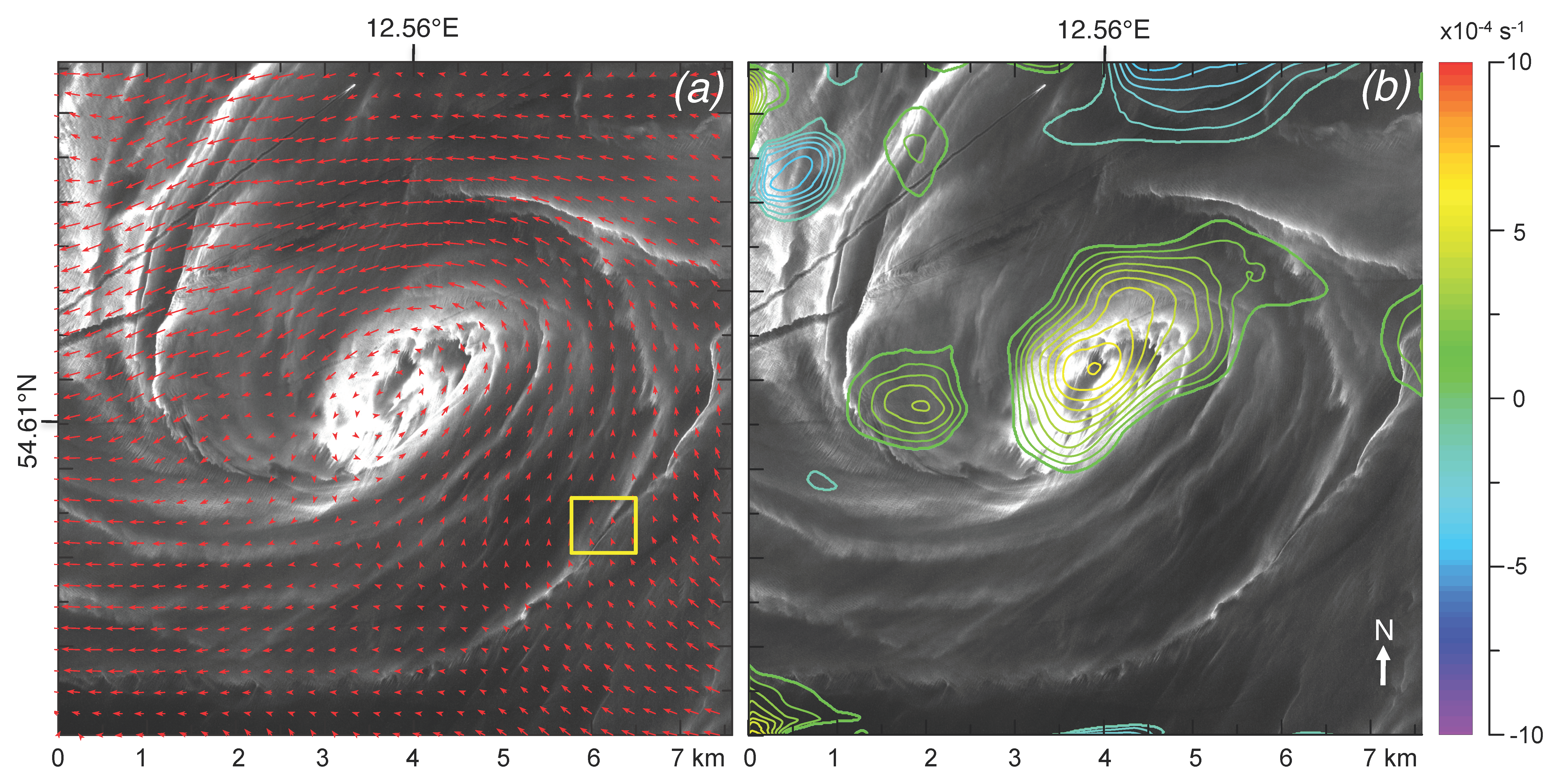
The dashed line in Figure 3a highlights a band of positive vorticity (horizontal shear) that lies to one side but parallels the aggregation. Spatially averaging in a 20-m wide strip along the dashed line yields a cyclonic vorticity of 4.81 × 10⁻⁴ s−1 (s.d. = 1.07 × 10⁻⁴ s−1). The dashed line in Figure 3b connects areas of negative divergence that overlay the aggregation. The mean divergence is −2.9 × 10⁻⁴ s−1 (s.d. = 1.42 × 10⁻⁴ s−1), and hence indicates surface convergence. These bands of vorticity and convergence indicate a velocity front. This supports an assumption made in the literature that such algal aggregations are frontal convergence zones and thus mark the locations of downwelling, i.e., that submesoscale convergence occurs within specific structures in the flow field [10]. Drifter measurements made in such structures show convergences of 2 to 6 f [10]; our value yields 2.4 f.
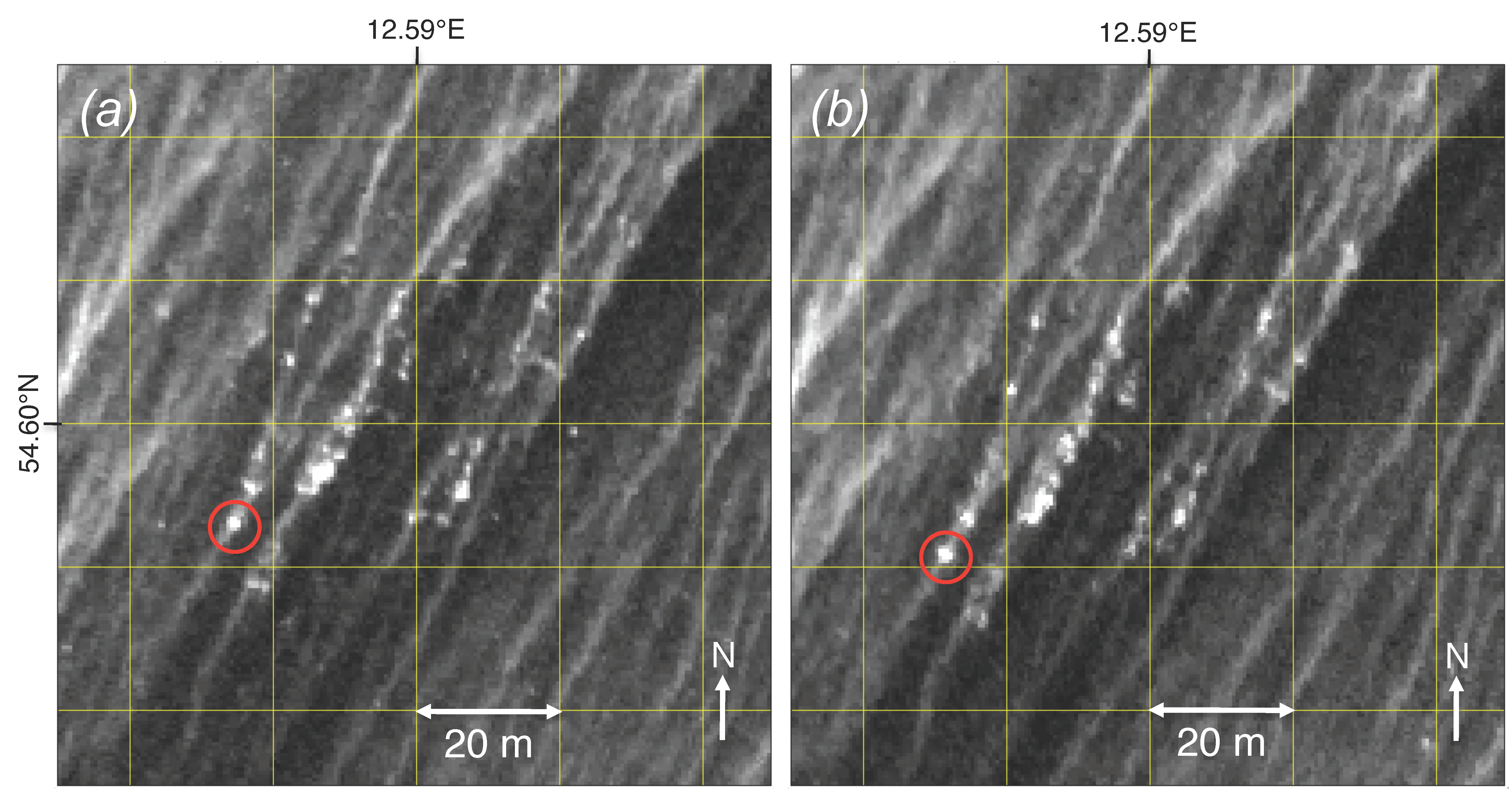
The windrows in Figure 3 are likely algae accumulations resulting from surface convergence created by Langmuir circulation cells [24,25]. Evidence for this is that the windrows are approximately aligned with the wind, i.e., they have an orientation of about 30°, which is within about 10° of the wind direction in the hour preceding image acquisition (Section 2.1). The spacing of the windrows in these data is in the range of 5 to 8 m, which would imply a mixing layer of 2.5 to 4 m depth. Amongst the windrows are a variety of relatively weak vorticity and divergence features, but an adjacent pair of negative and positive vorticity and divergence features (A and B in Figure 3a,b) stands out. These features can be accounted for as follows. Figure 4 shows an enlarged view of the area at times t1 and t2. The two views have been aligned using the windrow patterns; and, by referencing to a common set of grid lines, one can see that windrows patterns are indeed approximately stationary. On the other hand, numerous bright pixels near the middle of the scene, and associated with individual windrows, do move between views—by about 5 m, which corresponds to a relative speed of 0.06 m s−1, or about 1% of the wind speed. Bright pixels such as in this figure have an enhanced response in the WorldView near-infrared bands, and that response is characteristic of surface cyanobacteria [26]. The bright pixels are thus assumed to correspond to small clumps of floating algae, and these clumps are likely to be affected by both the wind-drift layer and wind drag on parts of the clumps that extend above the sea surface. The enhanced speed of the clumps is detected by the optical-flow analysis and gives rise to the dipolar vortices (A, B) in Figure 3a, and areas of divergence (A) and convergence (B) in Figure 3b as the flow first accelerates upwind of the clumps and then slows downwind. These fine-scale (~100 m) flow variations might, if desired, be suppressed by using the near-infrared response of the algae clumps to mask them prior to the velocity computation.
4. Conclusions
Very high-resolution, time-lagged satellite imagery has been used to examine aspects of small-scale ocean dynamical features as revealed through a cyanobacteria bloom in the western Baltic Sea. In this case, a single pair of along-track stereo WorldView images was analyzed using an optical-flow algorithm to derive fields of velocity, vertical vorticity, and horizontal divergence. The results show (we believe for the first time) that an algal spiral pattern has at its center a cyclonic vortex, and that an individual algal aggregation corresponds to a velocity front having both horizontal shear and convergence (and hence, downward transport). While some sources of processing and environment noise have been identified, further attention is needed for identifying and quantifying noise in the derived flow field. Despite these shortcomings, the approach examined here is generally applicable, as previous studies using WorldView imagery analyzed with the same optical-flow algorithm have shown it provides a new way to quantify spatially complex phenomena and to assess the fidelity of high-resolution coastal circulation models [8,9].
Supplementary Materials
The following are available online at https://0-www-mdpi-com.brum.beds.ac.uk/2072-4292/11/7/865/s1.
Author Contributions
G.M. conceived the idea for this study and drafted the manuscript. W.C. analyzed the imagery using his Global Optimal Solution algorithm, and contributed to the writing of the final draft.
Funding
This work was supported by the Office of Naval Research under Naval Research Laboratory (NRL) Project 72-1C02-09.
Acknowledgments
Data from the FINO-2 platform were provided courtesy of the BMWi (Bundesministerium fuer Wirtschaft und Energie, Federal Ministry for Economic Affairs and Energy) and the PTJ (Projekttraeger Juelich, project executing organization). This is contribution NRL/JA/7230-19-0341.
Conflicts of Interest
The authors declare no conflict of interest.
References
- Kääb, A.; Leprince, S. Motion detection using near-simultaneous satellite acquisitions. Rem. Sens. Environ. 2014, 154, 164–179. [Google Scholar] [CrossRef] [Green Version]
- Qazi, W.A.; Emery, W.J.; Fox-Kemper, B. Computing ocean surface currents over the coastal California current system using 30-min-lag sequential SAR images. IEEE Trans. Geosci. Rem. Sens. 2014, 52, 7559–7580. [Google Scholar] [CrossRef]
- Matthews, J.P.; Yoshikawa, Y. Synergistic surface current mapping by spaceborne stereo imaging and coastal HF radar. Geophys. Res. Letts. 2012, 39. [Google Scholar] [CrossRef] [Green Version]
- Gade, M.; Seppke, B.; Dreschler-Fischer, L. Mesoscale surface current fields in the Baltic Sea derived from multi-sensor satellite data. Int. J. Remote Sens. 2012, 33, 3122–3146. [Google Scholar] [CrossRef]
- Chen, W. A global optimal solution with higher order continuity for the estimation of surface velocity from infrared images. IEEE TGRS 2010, 48, 1931–1939. [Google Scholar]
- Chen, W. Nonlinear inverse model for velocity estimation from an image sequence. J. Geophys. Res. 2011, 116, C06015. [Google Scholar] [CrossRef]
- Chen, W.; Mied, R.P. River velocities from sequential multispectral remote sensing images. Water Resour. Res. 2013, 49, 3093–3103. [Google Scholar] [CrossRef] [Green Version]
- Delandmeter, P.; Lambrechts, J.; Marmorino, G.O.; Legat, V.; Wolanski, E.; Remacle, J.F.; Chen, W.; Deleersnijder, E. Submesoscale tidal eddies in the wake of coral islands and reefs: Satellite data and numerical modelling. Ocean Dyn. 2017, 67, 897–913. [Google Scholar] [CrossRef]
- Marmorino, G.; Chen, W.; Mied, R.P. Submesoscale Tidal-Inlet Dipoles Resolved Using Stereo WorldView Imagery. IEEE Geosci. Rem. Sens. Lett. 2017, 14, 1705–1709. [Google Scholar] [CrossRef]
- D’Asaro, E.A.; Shcherbina, A.Y.; Klymak, J.M.; Molemaker, J.; Novelli, G.; Guigand, C.M.; Haza, A.C.; Haus, B.K.; Ryan, E.H.; Jacobs, G.A.; et al. Ocean convergence and the dispersion of flotsam. Proc. Natl. Acad. Sci. USA 2018, 115, 1162–1167. [Google Scholar] [CrossRef] [Green Version]
- Taylor, J.R. Accumulation and subduction of buoyant material at submesoscale fronts. J. Phys. Oceanogr. 2018, 48, 1233–1241. [Google Scholar] [CrossRef]
- Huisman, J.; Codd, G.A.; Paerl, H.W.; Ibelings, B.W.; Verspagen, J.M.; Visser, P.M. Cyanobacterial blooms. Nature Rev. Microbiol. 2018, 16, 471. [Google Scholar] [CrossRef]
- Kahru, M. Using satellites to monitor large-scale environmental change: A case study of cyanobacteria blooms in the Baltic Sea. In Monitoring Algal Blooms: New Techniques for Detecting Large-Scale Environmental Change; Springer: Berlin, Germany, 1997; pp. 43–61. [Google Scholar]
- Flohr, P.; Vassilicos, J.C. Accelerated scalar dissipation in a vortex. J. Fluid Mech. 1997, 348, 295–317. [Google Scholar] [CrossRef]
- Updike, T.; Comp, C. Radiometric Use of WorldView-2 Imagery; Tech. Note; DigitalGlobe Inc.: Longmont, CO, USA, 2010. [Google Scholar]
- Corsini, G.; Diani, M.; Walzel, T. Striping removal in MOS-B data. IEEE Trans. Geosci. Rem. Sens. 2000, 38, 1439–1446. [Google Scholar] [CrossRef]
- Lyon, P.E. An automated de-striping algorithm for Ocean Colour Monitor imagery. Int. J. Rem. Sens. 2009, 30, 1493–1502. [Google Scholar] [CrossRef]
- Schneider, C.A.; Rasband, W.S.; Eliceiri, K.W. NIH Image to ImageJ: 25 years of image analysis. Nat. Methods 2012, 9, 671. [Google Scholar] [CrossRef]
- Karimova, S.; Gade, M. Improved statistics of sub-mesoscale eddies in the Baltic Sea retrieved from SAR imagery. Int. J. Rem. Sens. 2016, 37, 2394–2414. [Google Scholar] [CrossRef]
- Karimova, S. Spiral eddies in the Baltic, Black and Caspian seas as seen by satellite radar data. Adv. Space Res. 2012, 50, 1107–1124. [Google Scholar] [CrossRef]
- Eldevik, T.; Dysthe, K.B. Spiral eddies. J. Phys. Oceanogr. 2002, 32, 851–869. [Google Scholar] [CrossRef]
- Fennel, W.; Seifert, T.; Kayser, B. Rossby radii and phase speeds in the Baltic Sea. Cont. Shelf Res. 1991, 11, 23–36. [Google Scholar] [CrossRef]
- Marmorino, G.; Smith, G.; North, R.; Baschek, B. Application of airborne infrared remote sensing to the study of ocean submesoscale eddies. Front. Mech. Eng. 2018, 4. [Google Scholar] [CrossRef]
- Thorpe, S.A. Langmuir circulation. Annu. Rev. Fluid Mech. 2004, 36, 55–79. [Google Scholar] [CrossRef]
- Szekielda, K.H.; Marmorino, G.O.; Maness, S.J.; Donato, T.F.; Bowles, J.H.; Miller, W.D.; Rhea, W.J. Airborne hyperspectral imaging of cyanobacteria accumulations in the Potomac River. J. Appl. Rem. Sens. 2007, 1, 013544. [Google Scholar]
- McKinna, L.I. Three decades of ocean-color remote-sensing Trichodesmium spp. in the World’s oceans: A review. Progr. Oceanogr. 2015, 131, 177–199. [Google Scholar] [CrossRef]
Figure 1.
(a) Conditions in the Western Baltic Sea on 1 July 2018 as measured by the OLCI sensor aboard the Sentinel-3 satellite (https://s3view.oceandatalab.com/). Red-filled circle shows location of research platform FINO-2 (winds and in-water data); yellow-filled circle (just south of study site) indicates a land-based weather station. (b) WorldView-2 RGB image of the area of the red rectangle in panel a, showing the spiral pattern that is the focus of this study.

Figure 2.
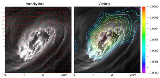
Results for area of the spiral pattern using data from band 3 (510 to 580 nm): (a) Velocity field; (b) Vorticity field. The largest vector in (a) has a magnitude of 0.21 m s−1. Contours in (b) are shown at an interval of 5 × 10⁻⁵ s−1, but only where the vorticity magnitude exceeds 1.5 × 10⁻⁴ s−1. A subset area (yellow rectangle; a) is examined in the next figure.
Figure 2.
Results for area of the spiral pattern using data from band 3 (510 to 580 nm): (a) Velocity field; (b) Vorticity field. The largest vector in (a) has a magnitude of 0.21 m s−1. Contours in (b) are shown at an interval of 5 × 10⁻⁵ s−1, but only where the vorticity magnitude exceeds 1.5 × 10⁻⁴ s−1. A subset area (yellow rectangle; a) is examined in the next figure.

Figure 3.
Example of algal aggregations in panchromatic data: (a) Vorticity; (b) Horizontal divergence. Contours are shown at an interval of 5 × 10⁻⁵ s−1, but only where the vorticity or divergence magnitude exceeds 1.5 × 10⁻⁴ s−1. Dashed lines and labeled features (A, B) are discussed in the text.
Figure 3.
Example of algal aggregations in panchromatic data: (a) Vorticity; (b) Horizontal divergence. Contours are shown at an interval of 5 × 10⁻⁵ s−1, but only where the vorticity or divergence magnitude exceeds 1.5 × 10⁻⁴ s−1. Dashed lines and labeled features (A, B) are discussed in the text.

Figure 4.
Enlargement of area near features A and B at times t1 (a) and t2 (b). The images shown here have been aligned using the windrow patterns. A common set of grid lines (spaced 20 m apart) helps illustrate how the brightest pixels (clumps of surface algae) move relative to the approximately stationary windrows. An example is circled in red and shows movement of about 5 m towards the south-southwest.

© 2019 by the authors. Licensee MDPI, Basel, Switzerland. This article is an open access article distributed under the terms and conditions of the Creative Commons Attribution (CC BY) license (http://creativecommons.org/licenses/by/4.0/).
Share and Cite
MDPI and ACS Style
Marmorino, G.; Chen, W. Use of WorldView-2 Along-Track Stereo Imagery to Probe a Baltic Sea Algal Spiral. Remote Sens. 2019, 11, 865. https://0-doi-org.brum.beds.ac.uk/10.3390/rs11070865
AMA Style
Marmorino G, Chen W. Use of WorldView-2 Along-Track Stereo Imagery to Probe a Baltic Sea Algal Spiral. Remote Sensing. 2019; 11(7):865. https://0-doi-org.brum.beds.ac.uk/10.3390/rs11070865
Chicago/Turabian StyleMarmorino, George, and Wei Chen. 2019. "Use of WorldView-2 Along-Track Stereo Imagery to Probe a Baltic Sea Algal Spiral" Remote Sensing 11, no. 7: 865. https://0-doi-org.brum.beds.ac.uk/10.3390/rs11070865
Note that from the first issue of 2016, this journal uses article numbers instead of page numbers. See further details here.