Temporal Up-Sampling of Planar Long-Range Doppler LiDAR Wind Speed Measurements Using Space-Time Conversion

Abstract

Measurement campaigns in wind energy research are becoming increasingly complex, which has exacerbated the difficulty of taking optimal measurements using light detection and ranging (LiDAR) systems. Compromises between spatial and temporal resolutions are always necessary in the study of heterogeneous flows, like wind turbine wakes. Below, we develop a method for space-time conversion that acts as a temporal fluid-dynamic interpolation without incurring the immense computing costs of a 4D flow solver. We tested this space-time conversion with synthetic LiDAR data extracted from a large-eddy-simulation (LES) of a neutrally stable single-turbine wake field. The data was synthesised with a numerical LiDAR simulator. Then, we performed a parametric study of 11 different scanning velocities. We found that temporal error dominates the mapping error at low scanning speeds and that spatial error becomes dominant at fast scanning speeds. Our space-time conversion method increases the temporal resolution of the LiDAR data by a factor 2.4 to 40 to correct the scan-containing temporal shift and to synchronise the scan with the time code of the LES data. The mean-value error of the test case is reduced to a minimum relative error of 0.13% and the standard-deviation error is reduced to a minimum of 0.6% when the optimal scanning velocity is used. When working with the original unprocessed LiDAR measurements, the space-time-conversion yielded a maximal error reduction of 69% in the mean value and 58% in the standard deviation with the parameters identified with our analysis.

1. Introduction

The arrangement of wind turbines into dense and efficient clusters is a central challenge in the design of wind farms. The detrimental effect of wake shading decreases energy yield and increases dynamic loads [1,2]. These additional loads lead to increased fatigue on the turbine components, increasing the likelihood of failure and early maintenance [3,4]. This additional and unexpected maintenance will deteriorate the economic and energy efficiency of the wind farm [5].

Wake models were developed early in the history of wind-turbine design to account for the loss of yield, wake-induced loads, and to aid in the design of wind turbines. Since single-point measurements are limited to cup anemometers mounted on the turbines themselves or on meteorological masts, reference and validation data can usually only be applied in the form of time averages [6,7,8].

Since wakes have highly dynamic behaviour, dynamic wake models have been developed for the sake of simulating how the wake meanders over time, to generate more realistic inflow conditions for load calculations in the design phase or for wind farm control. The dynamic wake meandering model (DWM) of Larsen et al. [9], which is unique in its method for simulating meandering behaviour, has been updated and adjusted to ease comparisons with measured data [10,11]. However, in Larsen et al. [10] and Churchfield et al. [11], a previously reported simulation of wake meandering from Larsen et al. [9] was used. Keck et al. [12] introduced a stochastic approach that considers meandering as it is related to atmospheric stability. Validation of these dynamic wake models requires wind velocity data collected with high spatial and temporal resolution, either from suitably recorded measurements or from high-fidelity computational fluid dynamics (CFD) simulations.

One of the most promising measuring devices for understanding wakes in free-field conditions is wind-speed Doppler light detection and ranging (LiDAR). LiDARs are configured as continuous-wave (CW) devices for short distances (<200 m) [13] or as pulsed systems for longer distances (<6000 m) [14]. Though LiDAR is commonly used for free-field measurements, Van Dooren et al. [15] took LiDAR measurements in a wind tunnel under controlled conditions in order to investigate wake behaviour using a synchronised dual-short-range LiDAR setup. Van Dooren et al. [15] captured two-dimensional (2D) flow situations of a model wind farm with three turbines in the range of 20 s per horizontal scan. Bartl et al. [16] investigated how selected yaw misalignments affected wake properties by varying the inflow turbulence and shear in a wind tunnel. In experimental and numerical tests, atmospheric conditions are not trivial to reconstruct, especially the recreation of fluctuations of length scales larger than the turbine. Thus, CFD and wind-tunnel tests cannot replace measurements of a full-scale system in the full field, but instead extend the range of research possibilities.

Due to the measurement principle used, some limitations apply when using a single long-range LiDAR setup for full-scale wake measurements. In Section 2, we discuss the constraints due to the one-dimensionality of the measurements, which include the complications in volume averaging due to the laser pulse. We also discuss how all the scanning measurements must strike a compromise between spatial and temporal resolution. These restrictions apply to both CW and pulsed LiDAR systems.

A significant advantage of short-range CW systems over long-range systems is their high measurement frequency, which allows temporal processes to be captured on a shorter time scale. In contrast, pulsed devices can take measurements at multiple quasi-instantaneous positions along the laser beam at long range. This spatial distribution allows the flow pattern of one or many wind turbines to be mapped within one scan.

Depending on the scan-repetition time and the maximum measurement range, characteristic air parcels can be analysed in the form of flow structures at multiple times at different positions with successive scans. Thus, the advection speed of the parcels can be determined and conclusions about their behaviour can be drawn [17]. The reasonableness of the reconstruction must be considered for each application. Resource assessment places more emphasis on time-interval-based values, like 10-min average wind speed and the ambient turbulence intensity [18], than on more fine-grained high-resolution flow dynamics. The numerical and temporal resources required to reconstruct high-resolution flow dynamics are inconsistent with the resulting benefits. In contrast, high-resolution time series are required for the characterisation and validation of models of wake meandering. Larsen et al. [9], Bingöl et al. [19], and Trujillo et al. [20] used LiDAR-based wake wind-speed time series with moderate sampling frequencies, between 0.04 Hz and 0.06 Hz, in order to compare the wake deficit position with wake meander model predictions from the DWM [9].

However, when analysing wake measurements recorded with LiDAR systems, especially in connection with other measurements, high-resolution multidimensional wake measurement data is helpful for the sake of synchronisation and correlation with data about atmospheric or turbine conditions’ information, like stability indicators, wind shear, wind veer, turbine thrust, and turbine loads, measured at specific moments in time [21]. As measurement campaigns tend to become more and more complex to allow detailed analysis of flow situations [21], the limitations of long-range LiDAR systems need to be understood in detail. Specifically, researchers need to know how planar measurement results can be used as time series in addition to the standard mode of statistical averages. To the same end, data-processing methods that can overcome the limitations of individual measurement systems with sufficient accuracy must be improved.

The first objective of this paper is to produce synchronised temporal and spatial high-resolution up-sampled flow data. The secondary objective is to facilitate comparison of this flow data with LES reference data. This comparison requires that the dynamics of planar full-field wake measurements are compatible with data from wind-tunnel experiments or CFD simulations. Further, this full-scale measurement data can be used directly for the evaluation of temporally variable flow structures or dynamic wake models.

To this end, Section 2 reports our parametric study of the measurement frequency of numerically simulated LiDAR data from an LES wake flow field, to understand how the measurement parameters influence the mapping quality. In Section 3, we present a method for temporal fluid-dynamics interpolation based on space-time conversion, which improves the temporal resolution of long-range planar LiDAR data to a sub-measurement-time scale. With this improvement in the temporal resolution, the time shift within a scan can be corrected, and we can mutually synchronise distinct measurements independent of their sampling time or temporal resolution. In Section 4, we show how the mapping error of horizontal and vertical nacelle-mounted wake measurements shifts from a spatial to a temporal nature as the measurement frequency changes. This analysis addresses how the representation of the mean value and standard deviation is affected by retrospectively increasing the temporal resolution of planar long-range LiDAR measurements. The effects of propagation and implied restrictions are discussed in Section 5 and conclusions are drawn in Section 6. While the paper focuses mostly on the presentation of horizontal measurements, appendices include detailed figures that show the corresponding results for vertical measurements. The effects of temporal up-sampling of LiDAR scans with different angular velocities are detailed in supplementary online video material.

2. Planar LiDAR Data

LiDAR systems are subject to limitations inherent to their principle of operation. Single systems can only measure the so-called line-of-sight (LOS) velocity along the direction of the laser beam, which is calculated from the light backscattered from aerosols [22].

A major source of inaccuracy is the spatial resolution of LiDAR, which depends mainly on the pulse length. When using a pulsed laser in commercial devices, the spatial quantisation of the wind speed in the radial direction is in the range of approximately 30 m [23]. This quantisation limit leads to volume averaging within an assumed cylindrical probe volume. This characteristic of LiDAR measurements has already been studied for its effects in turbulence measurement during the early days of LiDAR wind measurements [23,24,25]. Depending on the mode of operation, a second volume-averaging effect can build up in the scanning direction while recording planar measurements. During free flow, the associated error is relatively small [26]. In strongly turbulent flow situations that are very inhomogeneous, such as wind-turbine wakes, stronger deviations arise [26]. To understand the errors in this case, Fuertes and Porté-Agel [27] studied the errors in scanned measurements caused by heterogeneity in temporally averaged wake measurements.

A further restriction on LiDAR technology, which also applies to all scanning measurements systems, is that the spatial and temporal resolution of the measurements is in a trade-off relationship. The slower the selected scan speed, the finer the spatial resolution and the longer the scan-repetition time. Within a scan, the velocities measured at each scan angle correspond to different time stamps within a certain interval. Even though a whole scan may be visualised as a single picture or frame, such an illustration is not physically based and may be misleading. To avoid this effect, planar LiDAR data is usually averaged under the assumption that the time shift within a scan is negligible when compared with the averaging time.

A serious obstacle to using LiDAR for measurements of wind farms lies in the limited temporal resolution, or rather in the ideal combination of temporal and spatial resolutions that cannot yet be achieved with LiDAR systems. When using a very slow scanning speed, flow measurements are not recorded frequently enough to give a sufficient representation of the fluctuating behaviour, which is why the errors are temporal in nature. When using a very fast scan, the quantisation of the flow is too coarse. In this case, small-scale flow structures cannot be mapped with sufficient accuracy, which leads to errors of a spatial nature. Between these extremes lies an optimal parameter set that can clearly depict spatial structures and temporal fluctuations in the flow.

A statistical approach can be used to determine the optimal parameters, and will guarantee that the recorded data is sufficient:

$$N_m\ge {\left(\frac{z{\sigma }_m}{e}\right)}^2,$$

(1)

where $N_m$ is the required number of scans, $z$ is the confidence interval, $e$ is the maximum tolerable error, and ${\sigma }_m$ is the standard deviation of the measurements [28]. The scan resolution or measurement frequency can be derived from the number of scans required to provide a statistical estimation of the mean value. The basic problem here is that the requisite standard deviation (${\sigma }_m$) is unknown. In practice, this value can be calculated from additional measurements taken by instruments, like sonic or cup anemometers, or it can be estimated from previous LiDAR measurements to select appropriate LiDAR measurement parameters, like the angular-scan resolution.

The theoretical consideration of an optimal parameter set clarifies that many planar LiDAR measurements are recorded sub-optimally and may be statistically under-determined. Furthermore, for continuously optimal measurements, the measurement resolution will need to be adapted continuously to the variability in the flow. This adaptation requires a re-assessment of the data analysis and indicates that complex data-processing methods are in need of development.

In this study, we used simulated LiDAR data synthesised with a large-eddy simulation (LES) run in a LiDAR simulator (Section 2.2) to improve the error evaluation. We performed a parametric study of the measurement frequency to address the challenge of optimal measurement settings that can be used in real LiDAR measurement campaigns that may use a broad spectrum of measurement frequencies. The measurement parameters and trajectories used in these simulations were based on a real LiDAR measurement campaign of an onshore wind farm near Brusow in northern Germany, recorded in 2015 [21]. In the following, we first discuss real measurement parameters, as they provide a foundation for the variations that we used to generate LiDAR data from the LES, which are described afterwards.

2.1. Measurement Trajectories

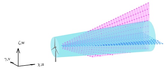
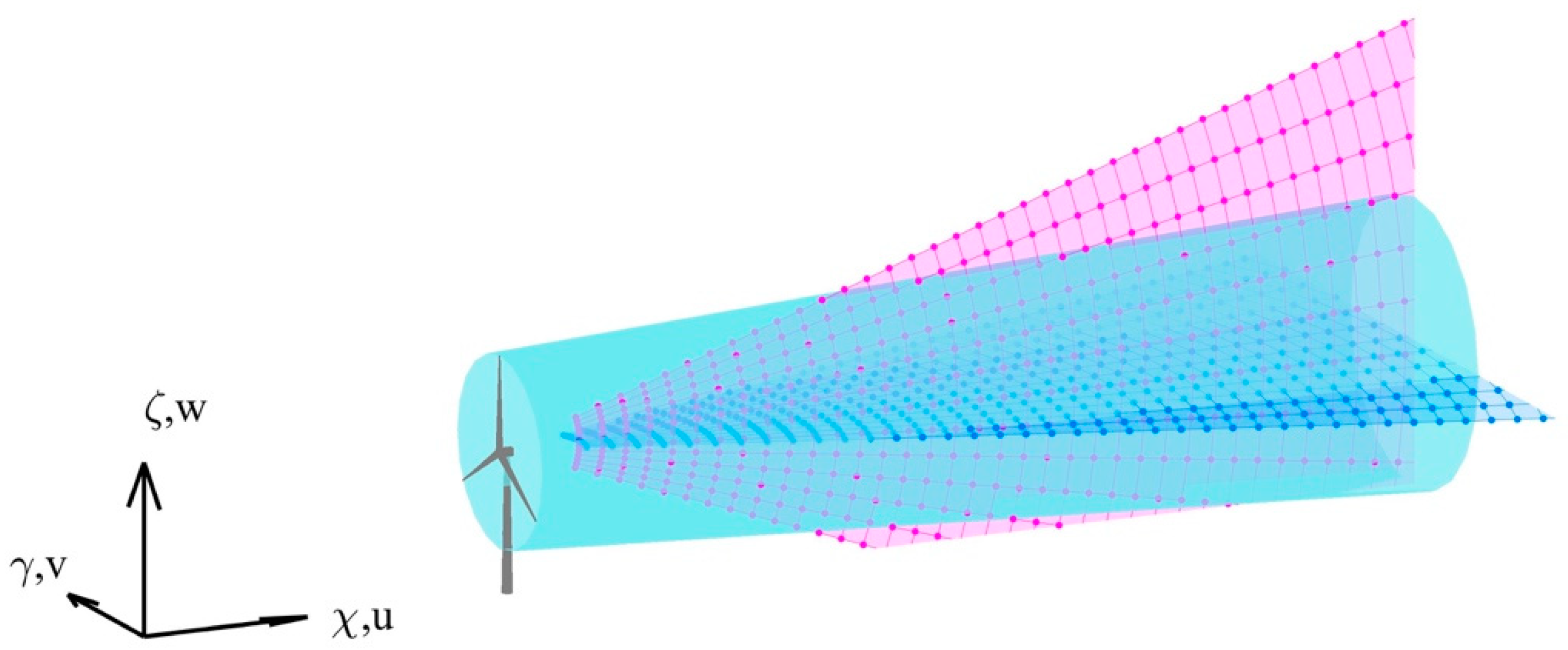
During the measurement campaign, we were fortunately able to position two long-range LiDAR devices on a single nacelle. At first, the measurement campaign in Brusow was intended for the improvement of commercial measurements, but instead aimed at a specific investigation of wake deflections caused by specific yaw misalignments. For this purpose, one device was used for horizontal plan position indicator (PPI) scans and the other was used for vertical range height indicator (RHI) scans. This combination of scans forms two unsynchronised perpendicular measurement planes in the downstream direction, which sliced the wake in horizontal and vertical directions, as illustrated in Figure 1. The installation of the LiDAR on the nacelle offers the advantage of reducing the measurement elevation for the horizontal scans relative to that of ground-based scans, and avoiding obstacles when adjusting the scan orientation to align with the direction of the wind.

Planar trajectories are executed either by fixing the elevation angle of the scanner ($\theta$) and continuously changing the azimuth angle ($\varphi$) (PPI) or by fixing the azimuthal scanner orientation while varying the elevation angle (RHI). PPI scans are typically executed with a full 360° azimuth range, and RHI scans are typically executed with a full 180° elevation range. In the configuration used in the present study, we performed only sectoral scan patterns, which we refer to as PPI and RHI below for the sake of readability. Since only sectors were measured, the scanning head requires some reset time ($t_r$) to return to its initial position. As no previous such measurements or studies about nacelle-based wake measurements were available, the scanning parameters used in the 2015 measurement campaign were not chosen specifically for certain atmospheric conditions, but they were instead chosen for their potential use as universal settings for volumetric nacelle-based wake measurements.

The structure of the LiDAR devices dictates that the measurement data is given in a spherical coordinate system that has the typical characteristics of a polar grid, in which the planar point density decreases as the measurement distance increases. The measurement grid is determined by the radial measurement points along the laser beam and the accumulation time due to the angular velocity in relation to the total opening angles, $\Delta \varphi$ and $\Delta \theta$. In the measurement trajectories that are actually executed, the total opening angles are defined symmetrically as:

$$\Delta \varphi =\left|{\varphi }_2-{\varphi }_1\right|,$$

(2)

$$\Delta \theta =\left|{\theta }_2-{\theta }_1\right|.$$

(3)

Measurement points were set in the radial direction in a range of 50 m to 1150 m at intervals of 7 m. During the measurements, we tested various accumulation times and found that ${\vartheta }_{acc}$ = 200 ms strikes a good compromise between the backscattering intensity and temporal resolution. The initial configuration for the angular speeds, ${\omega }_{\varphi }$ and ${\omega }_{\theta }$, was set to 2°/s, with total opening angles, $\Delta \varphi$ and $\Delta \theta$, of 40°. These settings yielded angular resolutions, ${ℛ}_{\varphi }$ and ${ℛ}_{\theta }$, of 0.4°.

2.2. Synthetic LiDAR Data

A large-eddy simulation based on the parallelized large-eddy simulation model (PALM) [29] and with the actuator line approach (ACL) [30] was used to calculate numerical approximations of the reference wake flow field behind the National Renewable Energy Lab’s 5-MW model wind turbine [31] with a rotor diameter ($D$) of 126 m. We decided to run this LES in an offshore environment since we did not plan to compare the real LiDAR data directly with the synthetic data. Furthermore, the simulation of the LiDAR measurement parameters is not affected by the choice between onshore or offshore conditions. The atmospheric conditions corresponded to a mean wind speed ($u_o$) of 8 m/s at a hub height of 92 m with an ambient turbulence intensity ($I_0$) of 5.8% at neutral stability. In these simulations, we used a 10-min time interval for the entire simulation, which therefore has a temporal resolution of 1 Hz and a spatial resolution of 10 m per grid cell in all three dimensions.

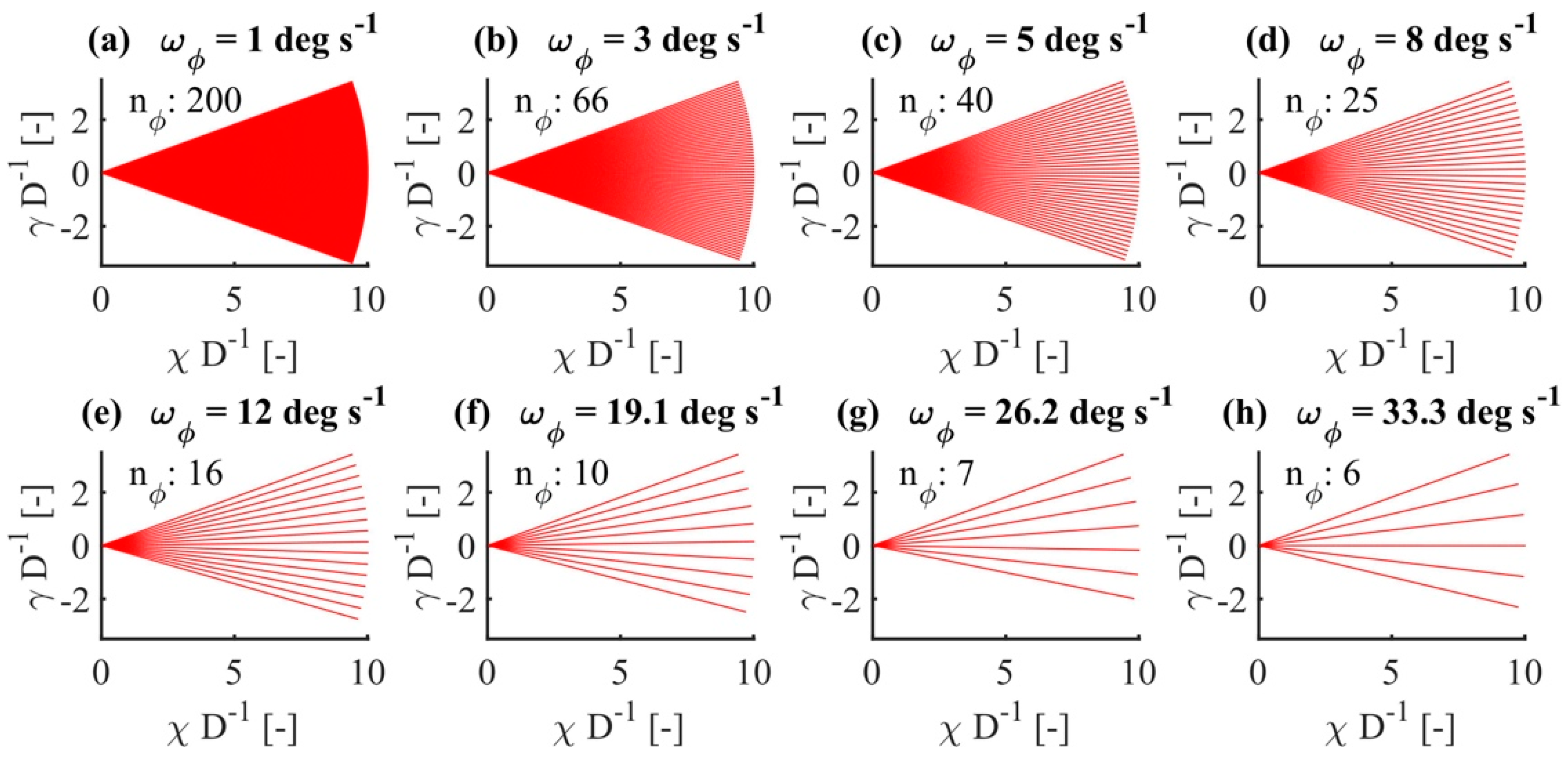
The varied parameter for the parametric analysis was the measurement frequency ($f_s$) as a function of the angular velocities, ${\omega }_{\varphi }$ and ${\omega }_{\theta }$. These parameters are listed in

Table 1. Simulated LiDAR trajectories of cross-measurements for $n_r=180$ and $\mathrm{T}=600\mathrm{s}$.

${\omega }_{\varphi }$, ${\omega }_{\theta }$	$\Delta \varphi$, $\Delta \theta$	${\mathrm{N}}_{\varphi }$, ${\mathrm{N}}_{\theta }$	$n_{pnt}$	$n_{\varphi }$, $n_{\theta }$	${ℛ}_{\varphi }$, ${ℛ}_{\theta }$	${\mathrm{T}}_{\varphi }$ ${\mathrm{T}}_{\theta }$	$f_s$	${\eta }_m$
1°/s	40°	15	36000	200	0.2°	40.0 s	0.024 Hz	97.2 %
2°/s	40°	29	18000	100	0.4°	20.0 s	0.047 Hz	94.2 %
3°/s	40°	42	11880	66	0.6°	13.3 s	0.068 Hz	91.0 %
4°/s	40°	54	9000	50	0.8°	10.0 s	0.089 Hz	89.2 %
5°/s	40°	66	7920	40	1.0°	8.0 s	0.011 Hz	86.8 %
6°/s	40°	77	6840	33	1.2°	6.7 s	0.127 Hz	84.6 %
8°/s	40°	97	4500	25	1.6°	5.0 s	0.161 Hz	80.6 %
12°/s	40°	133	2880	16	2.5°	3.3 s	0.221 Hz	73.4 %
19.11°/s	40°	183	1800	10	4.0°	2.1 s	0.303 Hz	63.4 %
26.22°/s	40°	221	1260	7	5.7°	1.5 s	0.370 Hz	55.8 %
33.33°/s	40°	250	1080	6	6.7°	1.2 s	0.417 Hz	50.0 %

. Figure 2 shows that the spatial resolution of the measurement grid of the trajectories has a significant effect. To make this data comparable to actual LiDAR measurement campaigns, we chose reasonable and realistic scan durations and extended them to approach the upper physical limits of common commercial long-range LiDAR devices. We selected a total of 11 different angular velocities for each value of ${\omega }_{\varphi }$ and ${\omega }_{\theta }$ and applied the accumulation time of ${\vartheta }_{acc}$ = 200 ms at the sampling frequencies of 0.024 to 0.417 Hz. The effect on the number of scans for each scan type within a 10-min interval (${\mathrm{N}}_{\varphi }$ and ${\mathrm{N}}_{\theta }$), the number of measurement points ($n_{pnt}$) for each scan type, the number of angular measurements per scan ($n_{\varphi }$ and $n_{\theta }$), the angular resolution (${ℛ}_{\varphi }$ and ${ℛ}_{\theta }$), the scan duration (${\mathrm{T}}_{\varphi }$ and ${\mathrm{T}}_{\theta }$), and the measurement-time efficiency (${\eta }_m$), all as a percentage of the total measurement time within a 10-min interval, are listed in Table 1. The coordinate system and the wind-speed components, as they are used below, are defined in Figure 1.

With the simulated measurement trajectories, we aimed to reproduce measurement points that are comparable to those in the measurement campaign and maintain the radial resolution of 7 m. The related choices result in an overlap of the pulses emitted by the LiDAR as 81.3% of the probe volume length of ~60 m. This resulted in the total number of radial ranges ($n_r$) being 180 at the radial distances of 1 to 1260 m. The point density of the Cartesian LES and the polar LiDAR measurement grid differ in the $\chi$ direction because of the radial spread of the angular measurements, which is illustrated in Figure 2. Thus, numerical redundancies while interpolating within LES grid cells can only be prevented with an extremely finely discretised wind field and the necessary numerical and temporal capacities were not available within the scope of this study. Since the spatial resolution of the LES with 10 m per grid cell is coarser than the 7-m radial resolution of the LiDAR simulation, the permanent interpolation of the LES grid onto the LiDAR grid restricts our results to realistic behaviours. We expect that the standard deviation of the simulated LiDAR measurement will be lower than that of free-field measurements because of the interpolation from the polar to the Cartesian grid, but the main cause of this difference in the standard deviation is the much lower accumulation time of the LiDAR at ${\vartheta }_{acc}=0.2\mathrm{s}$ compared to the temporal resolution of the LES at 1 Hz. This difference is critical, so we cannot ensure the absolute transferability of the results presented in Section 4 to real LiDAR measurements taken from a free field. Nevertheless, our analysis of the standard deviations gives some indication of trends in the wake behaviour.

However, to give simulated behaviour that is most similar to the full-scale measurements, we considered the reset time (${\mathrm{t}}_r$), which is needed by the LiDAR device to restart the trajectory. During this time, the LiDAR returns to the initial scanner position without recording any measurements. The repetition time of a scan is, therefore, the sum of the scan time (${\mathrm{T}}_{\varphi }$) and the reset time (${\mathrm{t}}_r$). The reset time (${\mathrm{t}}_r$) was derived from real LiDAR measurements and was set to ${\mathrm{t}}_r$ = 1.2 s for an opening angle of 40°. The following equations explain the formal relationship of the PPI and RHI trajectories. For the sake of brevity, only the PPI case is written out below:

$${\mathrm{T}}_{\varphi }=\frac{\Delta \varphi }{{\omega }_{\varphi }},$$

(4)

$$n_{\varphi }=\frac{{\mathrm{T}}_{\varphi }}{{\vartheta }_{acc}},$$

(5)

$${ℛ}_{\varphi }=\frac{\Delta \varphi }{n_{\varphi }},$$

(6)

$${\mathrm{N}}_{\varphi }=\lceil \frac{\mathrm{T}}{{\mathrm{T}}_{\varphi }}\rceil ,$$

(7)

$\mathrm{T}=600s$ in the present study.

$$n_{pnt}=n_{\varphi }·n_r,$$

(8)

$${\eta }_m=1-\frac{{\mathrm{t}}_r}{{\mathrm{T}}_{\varphi }},$$

(9)

$$f_s=\frac{1}{{\mathrm{T}}_{\varphi }+{\mathrm{t}}_r},$$

(10)

For the calculation of ${\mathrm{N}}_{\varphi }$ and ${\mathrm{N}}_{\theta }$, we rounded up the scans that began in the 10-min interval, but did not finish within the interval. This rounding was not applied when determining ${\eta }_m$ to visualise how the measurement time efficiency is changed by the different angular velocities.

We also normalised the coordinate system to the wind turbine rotor diameter ($D$).

We used the defined measurement trajectories listed in Table 1 when running the LIXIM LiDAR simulator developed at ForWind by Trabucchi [32], which was used by van Dooren et al. [33] to calculate velocity data from an LES wind field. In total, 2334 synthetic scans representing 11 different angular velocities were simulated within the same 10-min interval of the LES. As with the physical LiDAR measurements, the resulting velocity data are given in radial coordinates.

The limitations and peculiarities of numerically simulated LiDAR measurements have been investigated before. Stawiarski et al. [34] studied the errors that affect a simulated dual-Doppler LiDAR system. They found that the error in the determination of the radial velocity consists of a random error due to measurement inaccuracies caused by the speckle effect and detector noise, a systematic error due to the frequency shift of the laser, non-linear amplifiers, digitising errors and non-ideal noise statistics, and direction errors due to the imperfect adjustment of the LiDAR system and/or scanner movement. Together, these errors cause a projection error, like that described in Equation (14). Träumner et al. [35] used simulated data to investigate the ability of dual-Doppler LiDAR systems to estimate turbulence length scales. The use of a LiDAR simulator in the present study is meant to represent an ideal LiDAR which, apart from volume averaging, does not consider any other interference, as described by Stawiarski et al. [34]. This ideal simulation emphasises the peculiarities of the space-time conversion method discussed below.

Within the LIXIM software, we used the weighted average of the LOS velocity over the sample volume we considered. To this end, we defined a linear coordinate ($s$) in the beam direction and varied its orientation as shown in Figure 2 with different azimuth/elevation angles. The linear coordinate, $s$, represents the radial distance from the LiDAR to the measurement point. The range gate length corresponding to the spatial extension ($\Delta p=36\mathrm{m}$) and the Gaussian-formed laser pulse with intensity, $I_p$, characterised by a full-width at half-maximum ($\Delta r$) of 30 m [36] were used to calculate the LOS velocity:

$$I_p\left(s\right)=\frac{1}{\sqrt{\pi }\Delta r}{e}^{\left(-\frac{s^2}{\Delta r^2}\right)}.$$

(11)

The estimated LOS velocity is therefore:

$${\widehat{\upsilon }}_{LOS}\left(s\right)=\frac{1}{\Delta p}{{\displaystyle \int }}_{-\Delta p/2}^{+\Delta p/2}{\upsilon }_p\left(s\right)ds,$$

(12)

where:

$${\upsilon }_p\left(s\right)={{\displaystyle \int }}_{-k_p\frac{\Delta r}{2}}^{+k_p\frac{\Delta r}{2}}{\upsilon }_{r^{\prime }}\left(s^{\prime }-s\right)I\left(s^{\prime }-s\right)d{s}^{\prime },$$

(13)

with $I=\frac{I_p\left(s\right)}{{{\displaystyle \int }}_{-\infty }^{+\infty }{I}_p\left(s\right)ds}$ and $k_p=2.56$.

We are aware that the pulse intensity of a real LiDAR differs from the Gaussian representation in Equation (11), but Frehlich used a similar Gaussian distribution [24]. Stawiarski et al. [34] and Träumner et al. [35] used a similar weighting function. In other studies, the pulse shape was modelled with other approaches. Mann et al. [37] used an axisymmetric function that, according to Lindöw [38], reasonably approximates the distribution of the pulses emitted by the WindCube LiDAR system. Fuertes et al. [39] built on Mann et al. [37] for the pulse-weighting of a single LiDAR, but they used a 3D Gaussian function to evaluate three synchronised LiDAR measurements.

The choice of the laser pulse function directly affects the calculation of the LOS velocity. As can be deduced from Equation (11), the radial velocity component is a weighted average of the pulse geometry. This averaging in the beam direction affects the resulting velocity, as it is affected by the velocity shear within the pulse geometry. In a wind field with constant laminar wind speed, volume averaging would have no effect. The stronger and faster the velocity shear within the probe volume, however, the greater the error in the accumulated speed. This influences the representation of the mean value and the standard deviation, which will thereby be under-estimated in relation to the reference. Depending on the pulse shape that is assumed, volume averaging will have different effects.

As we used it, LIXIM was only able to calculate the spatial average in the radial direction, but not in the scanning direction. This provided deeper insight into step-and-stare measurements, in which the scanner stops and accumulates data for each measurement. This behaviour restricts the transferability of the resulting parameters to on-the-fly measurements, in which the scanner continuously accumulates data as it moves. LiDAR measurements are usually taken on-the-fly to optimise measurement efficiency in terms of the measurement time. To give some insight into the peculiarities of on-the-fly measurements, we will subsequently introduce a planar average that accounts for this effect in Section 4.1.1.

3. Method

3.1. Wind-Speed Reconstruction

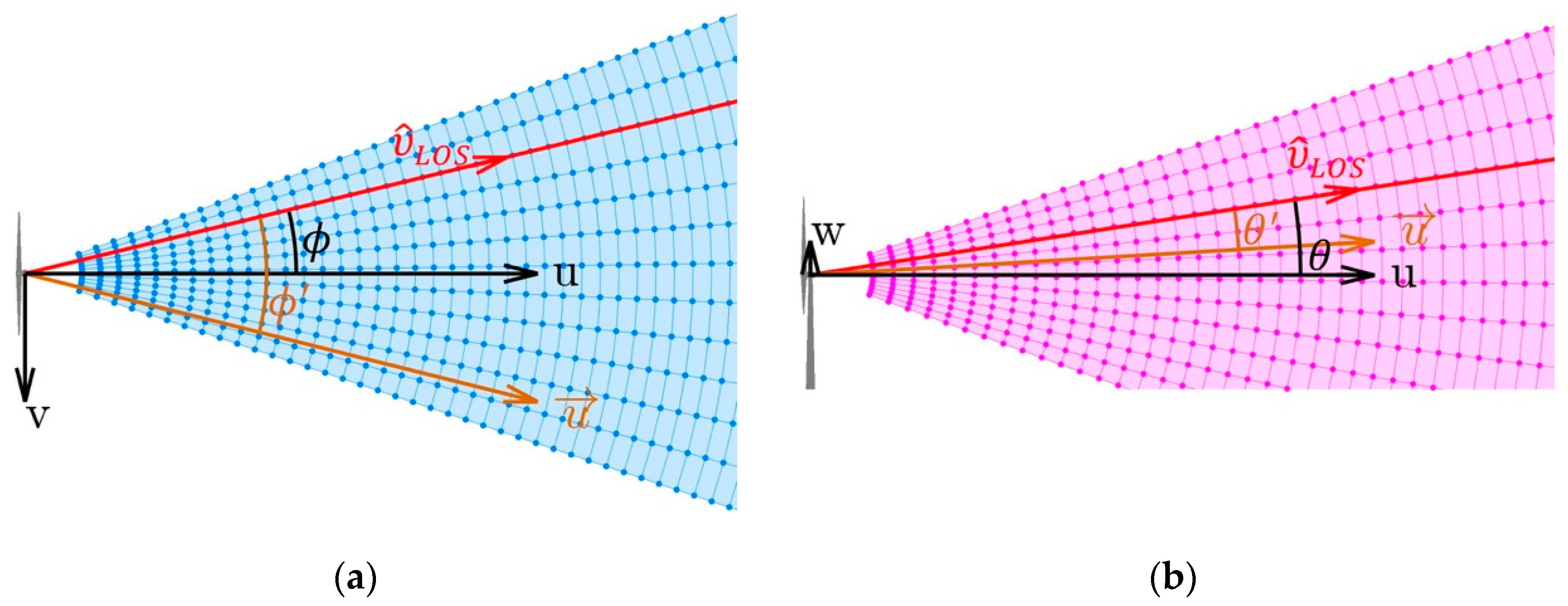
Since LiDAR provides 1D LOS velocities, we assume that horizontal and vertical wind directions are constant within the considered time interval ($\mathrm{T}$) of the flow field. Thus, the streamwise wind-speed component ($u$) can be constructed relative to an external source of wind direction:

$$u=\frac{{\widehat{\upsilon }}_{LOS}}{\cos \left({\varphi }^{\prime }\right)\cos \left({\theta }^{\prime }\right)},$$

(14)

where ${\varphi }^{\prime }$ is the difference between the horizontal wind direction, $\mathsf{\Phi }$, and the azimuth angle, $\varphi$, and ${\theta }^{\prime }$ is the difference between the vertical wind direction, $\mathsf{\Theta }$, and the elevation angle, $\theta$, as illustrated in Figure 3.

With nacelle-based measurements, we can assume that the wind direction tracking of the turbine is sufficiently good if no intentional yaw misalignment is present. Within the synthetic data, the lateral wind-speed component ($v$) and the vertical component ($w$) are assumed to average out to zero, though this assumption does not apply in the near-wake region ($\mathsf{\chi }{D}^{-1}\le 3$). Alternatively, the PPI scans we performed can be used to determine the wind direction at different downstream distances if we use the horizontal velocity azimuth display (VAD) fitting approach. In other cases, $\mathsf{\Phi }$ and $\theta$ can be determined with external wind direction instruments, such as vertical profilers using VAD or Doppler-beam-swing (DBS).

Below, we will calculate the average velocity and its standard deviation in the $u$ direction. This calculation applies Equation (14) to the time series of LOS velocities of each point within the measurement area. The resulting statistics do not allow us to reconstruct the exact streamwise wind-speed component statistics. Even so, the implied assumptions are unavoidable when using LiDAR data without other external information or reconstructions based on turbulence spectra. We are aware that our calculation of the standard deviation of the projected wind-speed component (${\sigma }_u$) differs from the standard deviation of the LOS velocities (${\sigma }_{{\widehat{\upsilon }}_{LOS}})$ for ${\varphi }^{\prime }\ne 0$ and ${\theta }^{\prime }\ne 0$ due to the non-linear dependence of the standard deviation of the LOS velocities (${\sigma }_{{\widehat{\upsilon }}_{LOS}})$ on the standard deviations of the main wind-speed components (${\sigma }_u$, ${\sigma }_v$, ${\sigma }_w$). Since the standard deviations of all wind-speed components in LiDAR measurements (${\sigma }_u$, ${\sigma }_v$, ${\sigma }_w$) represent unknowns with no additional external measurements, Equation (14) represents a pragmatic approach for projecting the LOS velocity time series onto the main wind direction, from which the standard deviation (${\sigma }_u$) can be compared with the standard deviation of the LES (${\sigma }_{u_{LES}}$).

The LOS velocities were projected scan-wise, and individual scans were interpolated onto a Cartesian (χ-γ or γ-ζ) coordinate grid using the natural-neighbour interpolation [40].

3.2. Wind-Field Propagation

For most wind speed analyses that aim to give wind speed averages, the recorded scans can be assumed to be quasi-instantaneous. The time shift within a scan is relatively small when compared to the total averaging time. In contrast, if certain dynamics will be calculated or derived from the wind-speed measurements, a high-resolution time series will be needed. If the measurement frequency of points within the measurement region is higher, the conclusions about the dynamics will be more accurate. When analysing scanned wake measurements, special attention must be paid to the temporal shift within a scan, as this temporal shift means that the scan does not show the flow situation at one moment, but instead covers a time interval. When scanning cross-wise in the flow direction, characteristic flow structures are distorted depending on their expansion and flow velocity. If the scan direction is parallel to the flow direction, flow structures may be distorted or may be imaged several times in a single scan, depending on the flow dynamics and scan velocity. This effect is relevant when determining the wake deficit of a wind turbine or when determining the dynamics at the centre of the wake in the downstream direction. Two aspirations are joined with this effect: (1) Our aim is to improve on the temporal resolution and (2) to give a temporally realistic representation of the scanned data. As Section 3.3 will show, the improvement of the temporal resolution improves the physical realism of the data.

Table 1 shows that planar scans are typically taken over intervals from 1.2 s to 40 s. The scan-repetition time limits the temporal scale of the data that can be analysed and synchronised with simultaneously measured data. As mentioned in Section 1, the correlation of flow structures with atmospheric or turbine-measured data is essential for identifying specific synergies in the LiDAR measurements.

The approach used in the following space-time conversion is chosen to meet the requirement that a characteristic flow situation be measured several times in sequence. Depending on the flow velocity and the measurement range, this limits the region in which wind-field propagation can be applied. According to the requirement that a flow situation be measured in two or more consecutive scans, we can use the laws of fluid dynamics to convert the spatial wind velocity information collected in a scan into temporally expressed information. This general idea has been used in other studies to interpolate or extrapolate flow situations from measurements or defined states. Schneiders and Scarano [41] reconstructed instantaneous flow fields from time-resolved volumetric particle tracking velocimetry (PTV) measurements using multidimensional velocity measurements and their derivatives. Their vortex-in-cell plus (VIC+) method relies on the calculation of vorticity, which in turn requires at least 2D velocity information, which cannot be collected with a single LiDAR system. Like the approach we describe below, Rott et al. [42] used a semi-Lagrangian advection scheme and a stepwise flow solver to estimate the available power during the curtailment of a wind farm by forecasting the flow dynamics and aerodynamic interactions between the turbines. Valldecabres et al. [43] applied the hypothesis of frozen turbulence [44] with local topographic corrections to forecast wind speeds at specific downstream positions from LiDAR measurements taken over the very-short term.

In this section, we propose a model that describes how the flow evolves between subsequent scans, which we then apply to achieve continuous closure of planar LiDAR data over time at a specific downstream position. This approach assumes that the measured air parcels evolve downstream along with the local streamwise velocity. This implies that the air parcels do not adhere to Taylor’s frozen turbulence hypothesis that assumes advection with a global mean velocity [44]. Like the approach of Rott et al. [42], the following approach can be described using a semi-Lagrangian scheme. At each time step ($t$), the velocity data on a grid point is interpreted as a parcel of air that is free to move with its own velocity ($u\in ℝ$) and direction ($\overrightarrow{u}\in S^1\subset {ℝ}^2$), with $S^1≔\left\{\left(\mathsf{\chi },\gamma \right)\in {ℝ}^2|\sqrt{{\mathsf{\chi }}^2+{\gamma }^2}=1\right\}$. This can be understood as an interpretation of Taylor [44] that applies to small spatial and temporal scales.

The advection of each parcel can be approximated in a discretised fashion using the following equations:

$$\frac{\partial u\left(\mathsf{\chi },\mathrm{t}\right)}{\partial t}=-u\left(\mathsf{\chi },\mathrm{t}\right)·\nabla u\left(\mathsf{\chi },\mathrm{t}\right),$$

(15)

$$u\left(\mathsf{\chi },t+\Delta t\right)=u\left(\mathsf{\chi },t\right)-\Delta t·u\left(\mathsf{\chi },t\right)·\frac{\delta u\left(\mathsf{\chi },\mathrm{t}\right)}{\delta \mathsf{\chi }},$$

(16)

$$u\left(\mathsf{\chi },t+\Delta t\right)=u\left(\mathsf{\chi },t\right)-\Delta t·u\left(\mathsf{\chi },t\right)·\frac{u\left(\mathsf{\chi },t\right)-u\left(\mathsf{\chi }-\Delta \mathsf{\chi },t\right)}{\Delta \mathsf{\chi }},$$

(17)

with $\frac{\mathsf{\Delta }\mathsf{\chi }}{\mathsf{\Delta }t}=u\left(\mathsf{\chi },t\right)$ respectively $\Delta \mathsf{\chi }=u\left(\mathsf{\chi },t\right)·\Delta t$. Note that this equation is given in only one dimension because it is projected on the affine subspace, $\mathsf{\chi }+\lambda \overrightarrow{u}\subset {ℝ}^2$, with $\lambda \in ℝ$. This representation gives:

$$u\left(\mathsf{\chi },t+\Delta t\right)=u\left(\mathsf{\chi },t\right)-\left(u\left(\mathsf{\chi },t\right)-u\left(\mathsf{\chi }-\Delta t·u\left(\mathsf{\chi },\mathrm{t}\right),t\right)\right),$$

(18)

$$u\left(\mathsf{\chi },t+\Delta t\right)=u\left(\mathsf{\chi }-\Delta t·u\left(\mathsf{\chi },\mathrm{t}\right),t\right),$$

(19)

where $\mathsf{\Delta }\mathsf{\chi }$ is the distance that the given air packet travels in one time step ($\Delta t$). If we define ${\mathsf{\chi }}_{old}≔\mathsf{\chi }-\Delta t·u·\overrightarrow{u}$ as the initial position of the packet on the regular Cartesian grid, Equation (19) shows that, at the next time step, $t_{new}≔t+\Delta t$, each parcel transports its own velocity and direction to its new location via advection ($\mathsf{\chi }={\mathsf{\chi }}_{old}+\Delta t·u·\overrightarrow{u}$). This means that parcels on the regular Cartesian grid are displaced to an irregular grid. To resolve the new velocity field in the original grid, the velocities in the intermediate grid are interpolated onto the initial grid using natural-neighbour interpolation [40].

To give an example of this method, we initialise this space-time conversion approach using a scan from Section 2.2 at $t_n$ and iterate it with selected temporal resolutions ($\Delta t$) to the time interval of the subsequent scan ($t_{n+1}$). Comparing the iterated and interpolated scans at $t_{n+1}$ with the processed LiDAR scan at $t_{n+1}$, the flow structures are subjected to numerical diffusion and smoothed out by the subsequent interpolation. To minimise the multiplication of errors with multiple iterations, we applied a mixed propagation approach with the temporal weighted average of forward- and backward-oriented propagations.

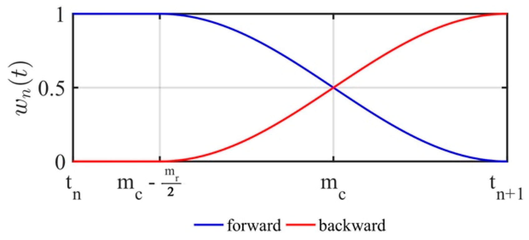
In the backwards-oriented propagation, we initialise the process with a negative time step ($-\Delta t$) that causes the air parcel at $t_{n+1}$ to propagate backwards in time to $t_n$. The sinusoidal function, $w_n\left(t\right)$, is used to calculate the weighted average of forward and backward propagations in order to minimise numerical diffusion and to guarantee continuous advection with no unphysical gaps.

We are aware that fluid-mechanical mixing processes are irreversible. We assume, however, that the spatial scale of the mixing process is considerably smaller than the spatial resolution of the measurements, so irreversibility is not a concern. We define $t\in \left\{ℝ|t_n\le t\le t_{n+1}\right\}$ and:

$$w_n\left(t\right)=\{\begin{array}{cc}1,& t\le m_c-\frac{m_r}{2}\hfill \\ \frac{1+\cos \left(\frac{\pi }{2}+\frac{\pi }{m_r}\left(\frac{t}{t_{n+1}}-m_c\right)\right)}{2},& m_c-\frac{m_r}{2}<t<m_c+\frac{m_r}{2}\hfill \\ 0,& m_c+\frac{m_r}{2}\le t\hfill \end{array}$$

(20)

Thus, the weighting function, $w_n\left(t\right)$, has total width of $t_{n+1}-t_n$ and gives variable results in the range from $t>m_c-\frac{m_r}{2}$ to $t<m_c+\frac{m_r}{2}$. The variable, $m_c$, serves as the point in time between $t_n$ and $t_{n+1}$ at which the weighting functions, $w_n\left(t\right)$, for forward propagation and $1-w_n\left(t\right)$ for backwards propagation are in equilibrium. The variable, $m_r=\frac{4}{5}\left(t_{n+1}-t_n\right)$, represents the centred window around $m_c=\frac{2}{5}{t}_n+\frac{3}{5}{t}_{n+1}$, within which $w_n\left(t\right)$ can take values between 1 and 0. Outside of $m_r$, the weighting function is either 1 or 0. The shift in the centre of the weighting function ($m_c$) towards $t_{n+1}$ suggests the greater effect of forward propagation compared with the backwards propagation, which accords with the irreversibility of the mixing processes. The behaviour of the weighting functions is illustrated in Figure 4. This treatment of $w_n\left(t\right)$ and the configuration of $m_r$ and $m_c$ were developed in an unpublished internal study that we will only outline briefly here.

Different approaches for mixing functions were tested in parametric studies to find the functions that give the smallest error of mixed propagation in comparison to the mean and standard deviation of the LES reference wind-speed values. We tested a linear approach, an exponential approach, and the trigonometric approach that we eventually used. The exponential increase in the error with each interpolation step was damped the most robustly when using the trigonometric function.

The definition of wind-field propagation implies that $\Delta t$ is the variable that determines the error. The number of interpolation steps (${\mathsf{\Pi }}_{\varphi }$, ${\mathsf{\Pi }}_{\theta }$) between two subsequent scans depends on this interval. We define the number of propagation steps between two scans as:

$${\mathsf{\Pi }}_{\varphi }=\left|\frac{T_{\varphi }+t_r}{\mathsf{\Delta }t}\right|,$$

(21)

with ${\mathsf{\Pi }}_{\varphi }\in \mathbb{N}$.

3.3. Temporal Correction and Data Synchronisation

Since planar LiDAR measurements are recorded with temporally distributed scans, each scan maps the evolution of flow over the scanning period. This temporal shift within the scan increases with longer scan duration, making scanned measurements difficult to compare with measurements that are presented in instantaneous form. The temporal correction method discussed in this section is intended to align the temporal shift within a scan so the flow situation at a single moment in time can be expressed. The refinement of the temporal resolution to scales less than that of the measurement, as introduced in Section 3.2, lays the foundation for the temporal correction.

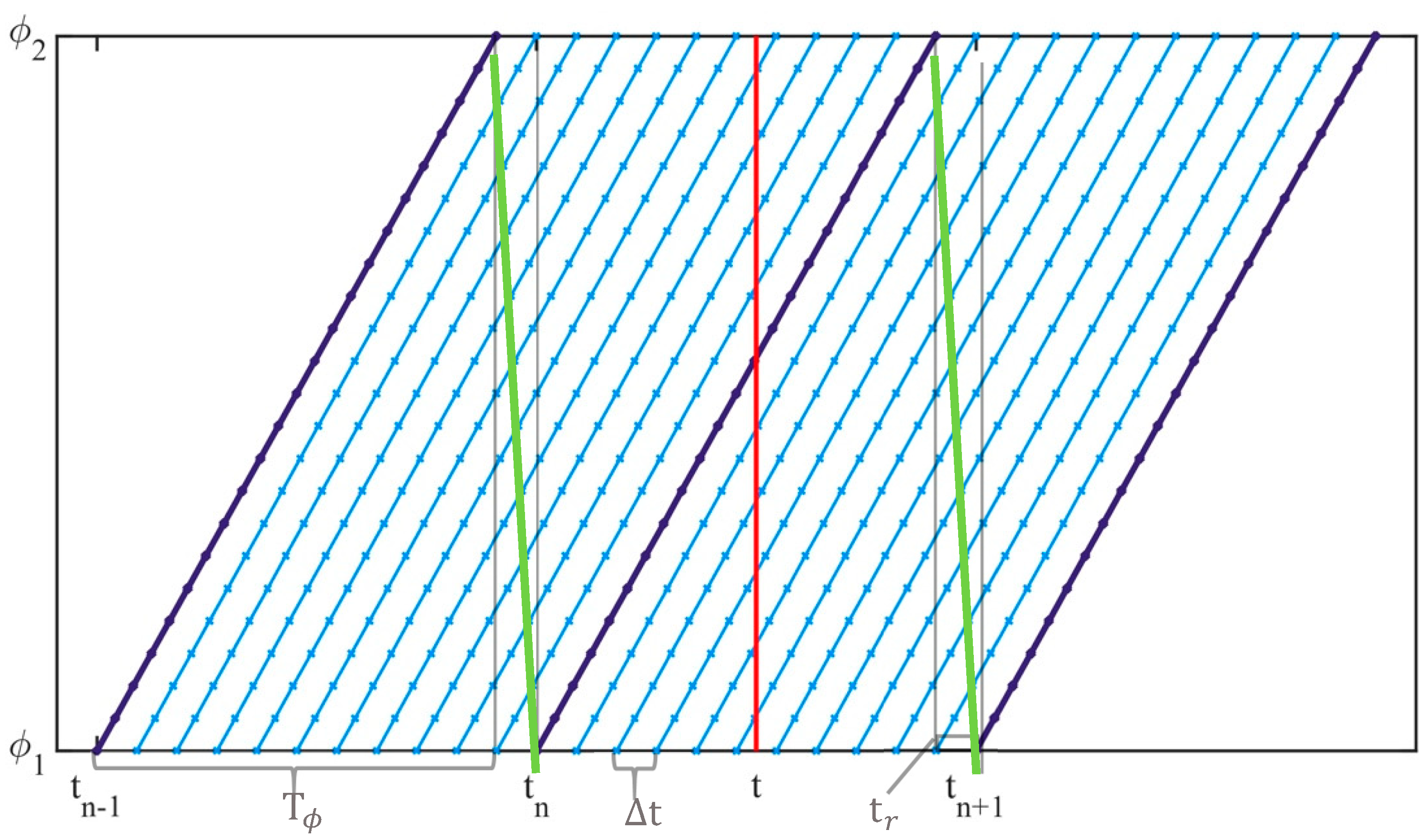
The time interval of each scan can be described as $T_n=\left[t_{n,1},t_{n,2}\right]≔\left\{t_{n,\mathsf{\chi }}\in T_n|t_{n,1}<t_{n,\mathsf{\chi }}<t_{n,2}\right\}$, where $t_{n,1}$ and $t_{n,2}$ are the beginning and end of the scan. Since the azimuth angle ($\varphi$) and the elevation angle ($\theta$) are functions of time, they can be expressed as $\varphi \left(t_{n,\mathsf{\chi }}\right)$ and $\theta \left(t_{n,\mathsf{\chi }}\right)$. As the time gaps between $\varphi \left(t_{n,\mathsf{\chi }}\right)$ and $\varphi \left(t_{n+1,\mathsf{\chi }}\right)$ and between $\theta \left(t_{n,\mathsf{\chi }}\right)$ and $\theta \left(t_{n+1,\mathsf{\chi }}\right)$ are closed with discrete interpolation steps because of the mixed wind-field propagation, 3D natural-neighbour interpolation can be applied at time $t$ [40]. The first two dimensions represent the scanned measurement area and the third dimension represents time. Figure 5 illustrates the temporal correction method and the 3D interpolation in 2D form, and the measurement area is represented as the scan angle, $\varphi \left(t\right)$, $\theta \left(t\right)$, over time. The propagation steps (light-blue lines) between two consecutive scans (dark-blue lines) are indicated by their slope, such that the measurement result and the refinement of the temporal resolution represent the measurement area over a time interval. By choosing the interpolation time step ($\Delta t$) carefully to give an integer number for interpolation ($\mathsf{\Pi }$), we can exclude the reset time of the scanner ($t_r$) (green lines), during which no measurements are captured. As shown in Figure 5, 3D interpolation is used to give the values of wind speed over the entire measurement area at the moment ($t$) (red line).

When a smaller value of $\Delta t$ is chosen, the temporal correction will have finer spatial resolution, since the spatial coverage is time-dependent. With the application of the temporal correction, measurements taken over a period of time can be interpolated into the same time and can thereby be synchronised to a single moment. Next, the RHI and PPI scans are synchronised to match the temporal resolution of the reference LES wind-field data.

The possibility of synchronising time-series data is not entirely novel. Cheynet et al. [45] shifted a time series of pulsed LiDAR data statically to a certain time using Taylor’s approach [44] to calculate the data’s coherence. While this approach retains the time-series dynamics, our method instead gives a new planar time series of data.

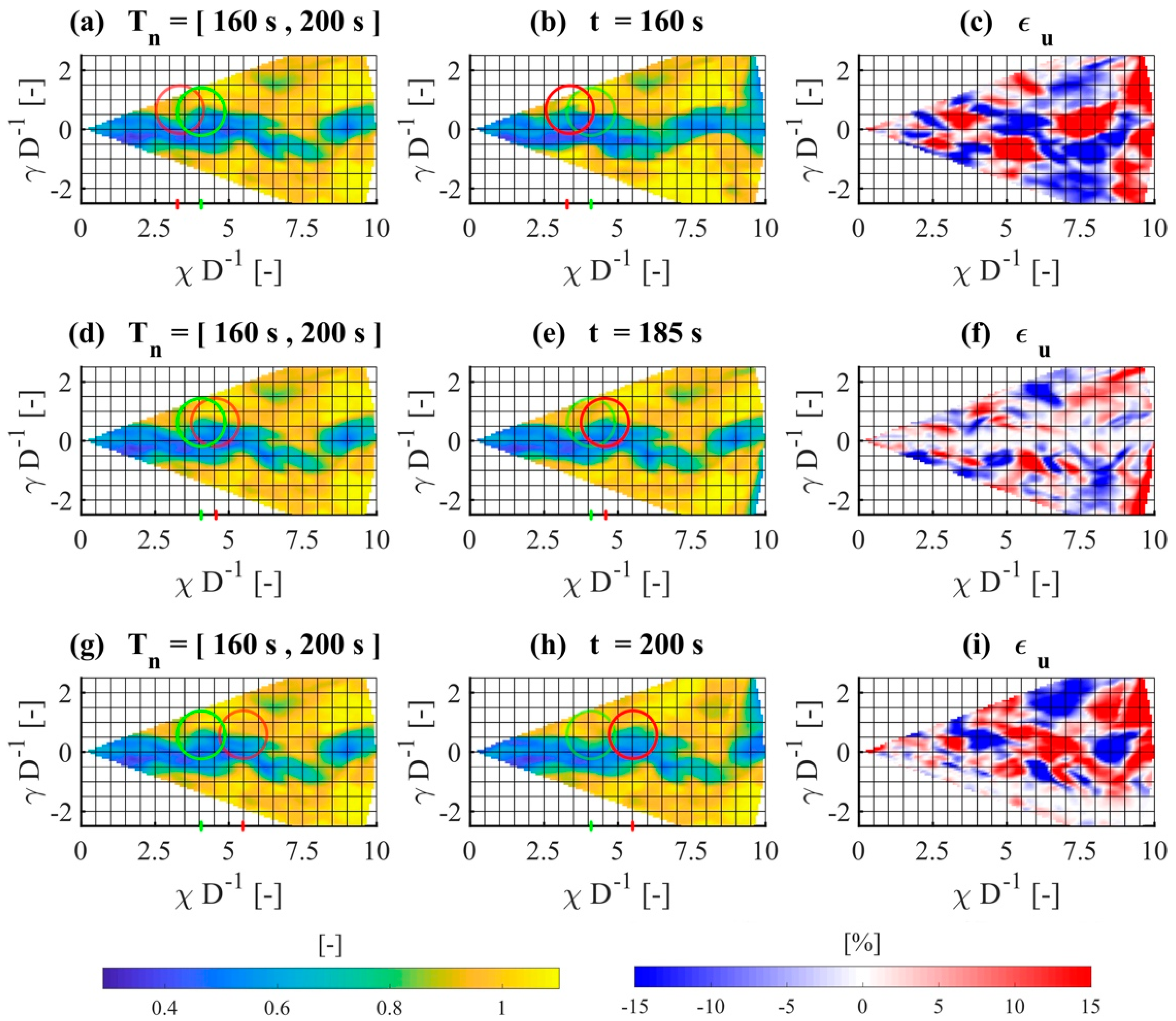
Figure 6 shows an example scan with ${\omega }_{\varphi }=1°/\mathrm{s}$, from which the effect of the temporal alignment can be seen within the planar scans. The first column (Figure 6a,d,g) shows the original LiDAR data measured in the time interval, $T_n=\left[160\mathrm{s},200\mathrm{s}\right]$. In the second column (Figure 6b,e,h), we see the temporal improved and corrected wake velocity data at the start of the scan at $t=160\mathrm{s}$ (Figure 6b), at the middle at $t=185\mathrm{s}$ (Figure 6e) and at the end at $t=200\mathrm{s}$ (Figure 6h). The third column (Figure 6c,f,i) visualises the instantaneous wind-speed deviations of the original LiDAR scan to the corrected data. While in the original scans, in Figure 6a,d,g, the green marked characteristic wake structures have the same downstream position for the time interval ($T_n$), it can be seen in the corrected data in Figure 6b,e,h that the positions of the red marked structures differ clearly from the green markings at individual points in time ($t$). We chose these three time points in order to show the effect of temporal alignment using the most common time sampling types, which set the time stamp either at the beginning of the measurement (Figure 6a–c), at the middle of the scan (Figure 6d–f), or at the end of the scan (Figure 6g–i). From the different positions of the green and red markers and with regard to the large wind-speed deviations in Figure 6c,f,i, we emphasise the relevance of the temporal correction again. However, the extent to which the temporal correction influences the results of the analysis of dynamic processes, like wake centre tracking or load time-series correlation, was not within the scope of the results in Section 4 and should be investigated in other studies.

4. Results

This section first discusses the results of the synthetic LiDAR data with different angular velocities (${\omega }_{\varphi }$) in Section 4.1. These results are related to the angular velocity instead of the measurement frequency, since the angular velocities are easier to differentiate in terms of typography. We describe the effects of the space-time conversion with different propagation time steps ($\mathsf{\Delta }t$) on the mean wind speed and its standard deviation in Section 4.2. For the sake of readability, we do not present detailed results of all the scan velocities we evaluated, instead illustrating only a selection of the data. We report all the results related to the RHI measurements in the appendix. We previously normalised all the wind speeds with a 10-min free-stream average and with the corresponding free-stream wind-speed profile, so the velocities are dimensionless in our presentation.

4.1. Calculation of Synthetic LiDAR Data

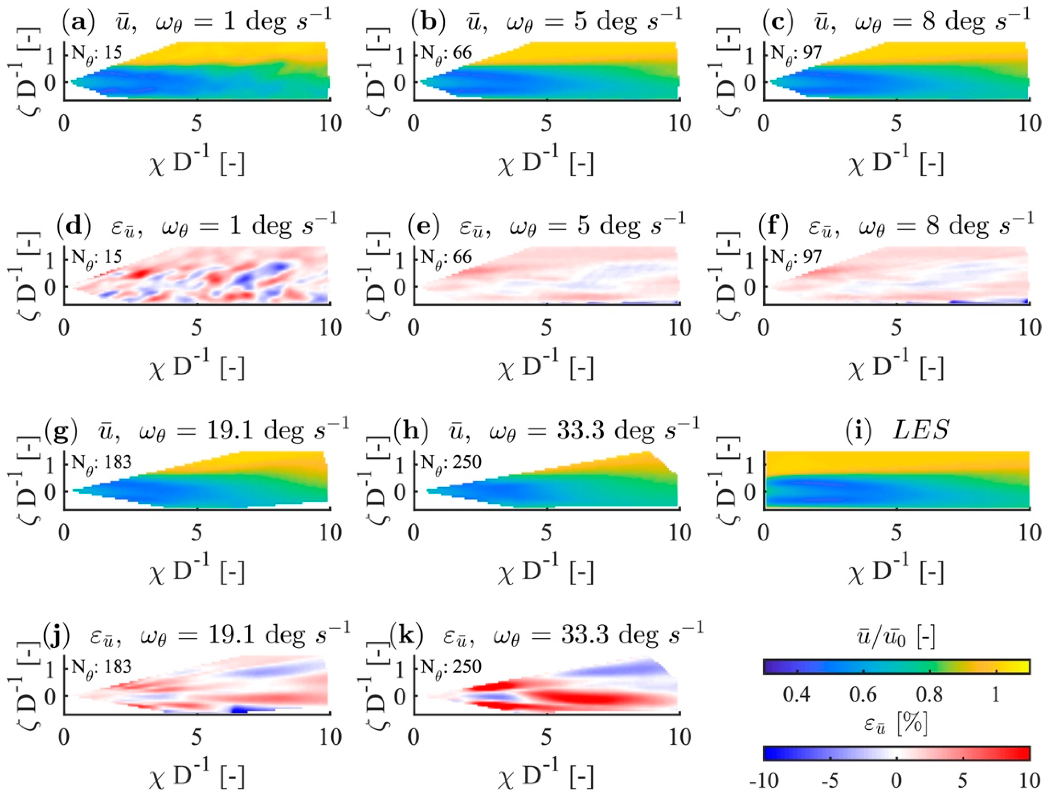
The LiDAR simulation was applied to synthesise a 10-min wake flow field, yielding the horizontal and vertical measurements summarised in Table 1. The resulting scanning times limit both the spatial and temporal resolution. One can see in these results how the choice of different scanning speeds affects the mapping accuracy of successive LiDAR scans. For error analysis, we evaluated the data at downstream distances of $4\le \mathsf{\chi }{D}^{-1}\le 9$ to compare this data with the propagated data described in Section 4.2. The RHI results that correspond to the data in Figure 7 and Figure 8 are presented in Appendix A. Nevertheless, in this section, we summarised the RHI data in Figure 9b.

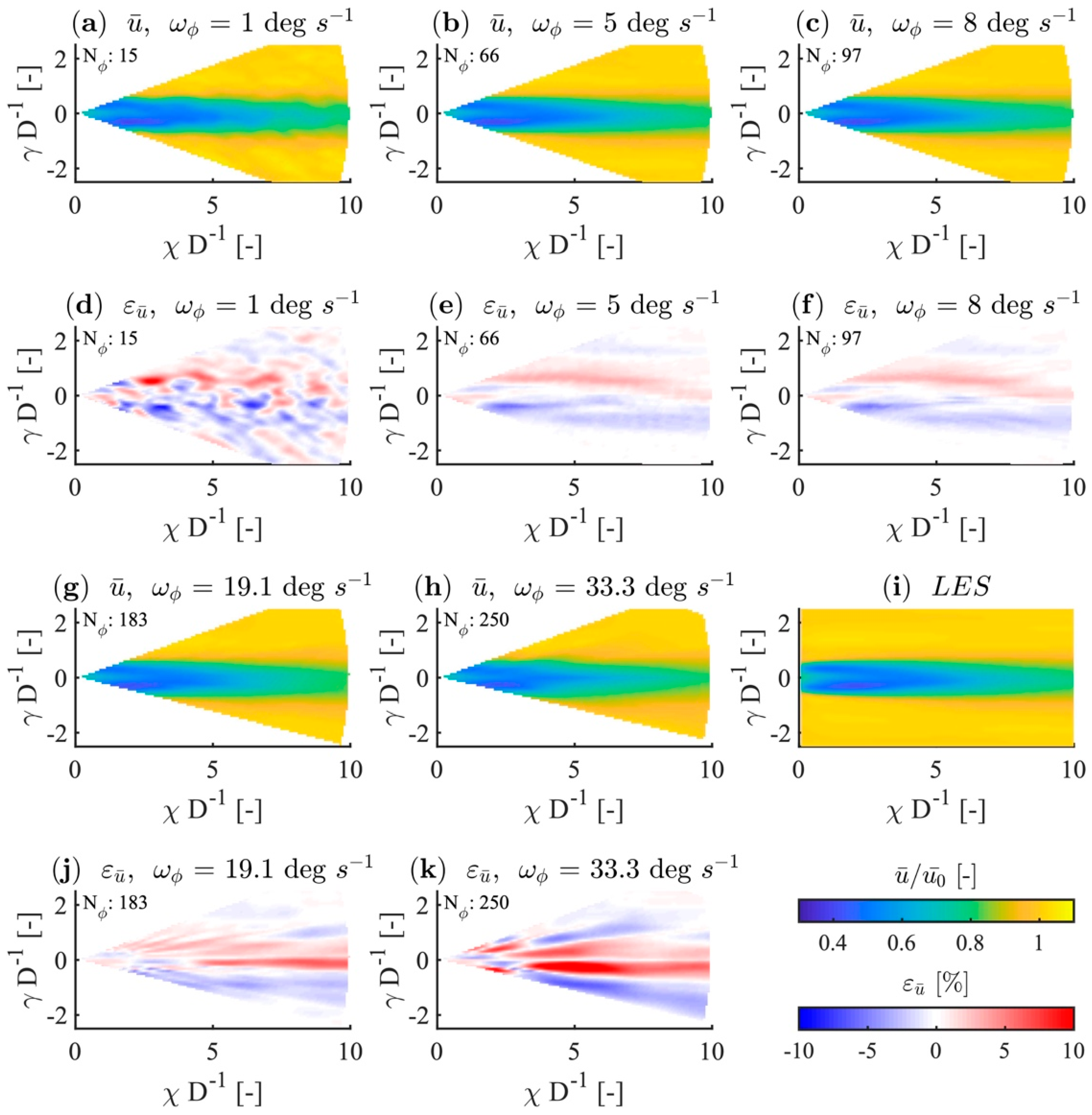
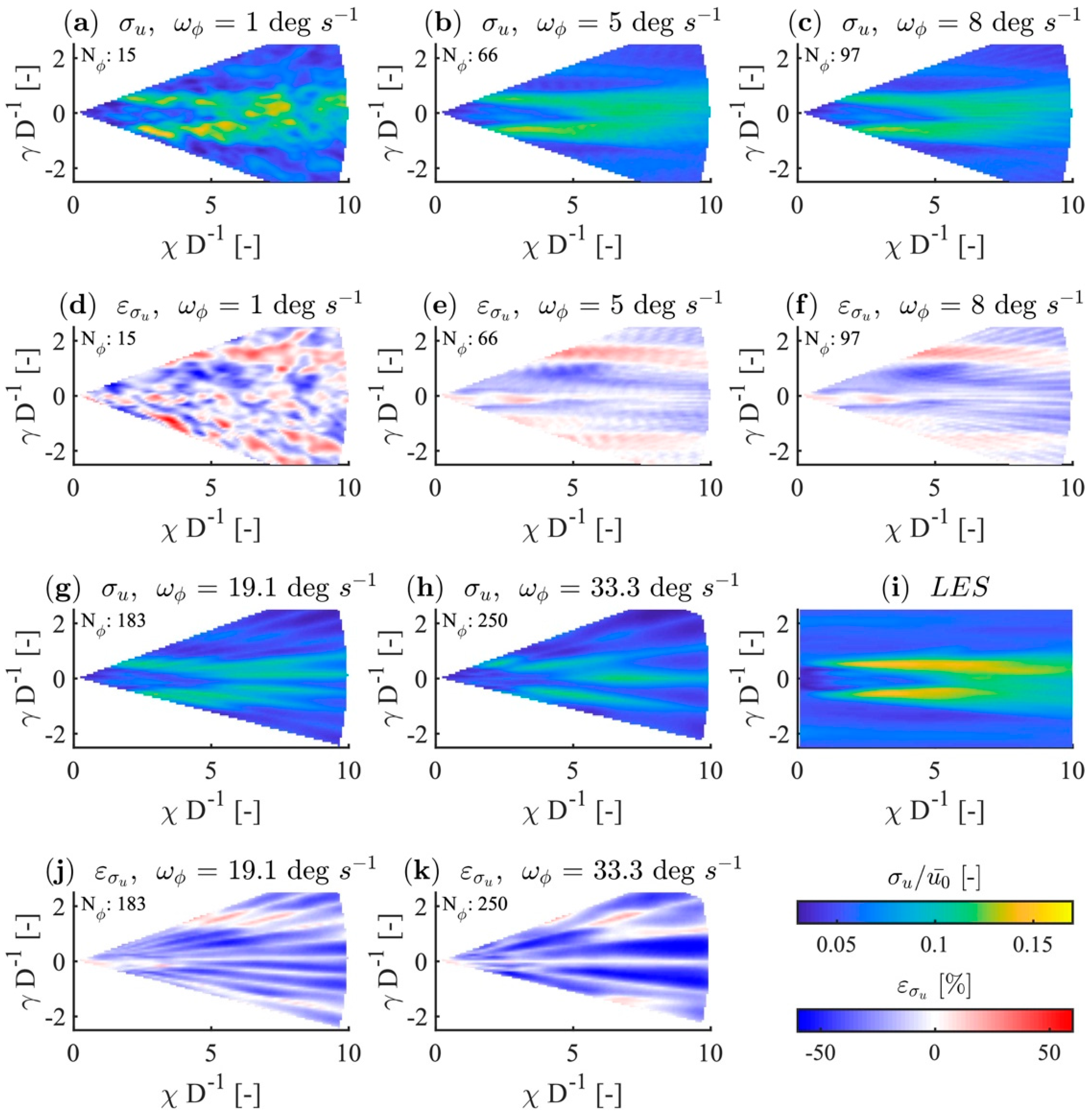
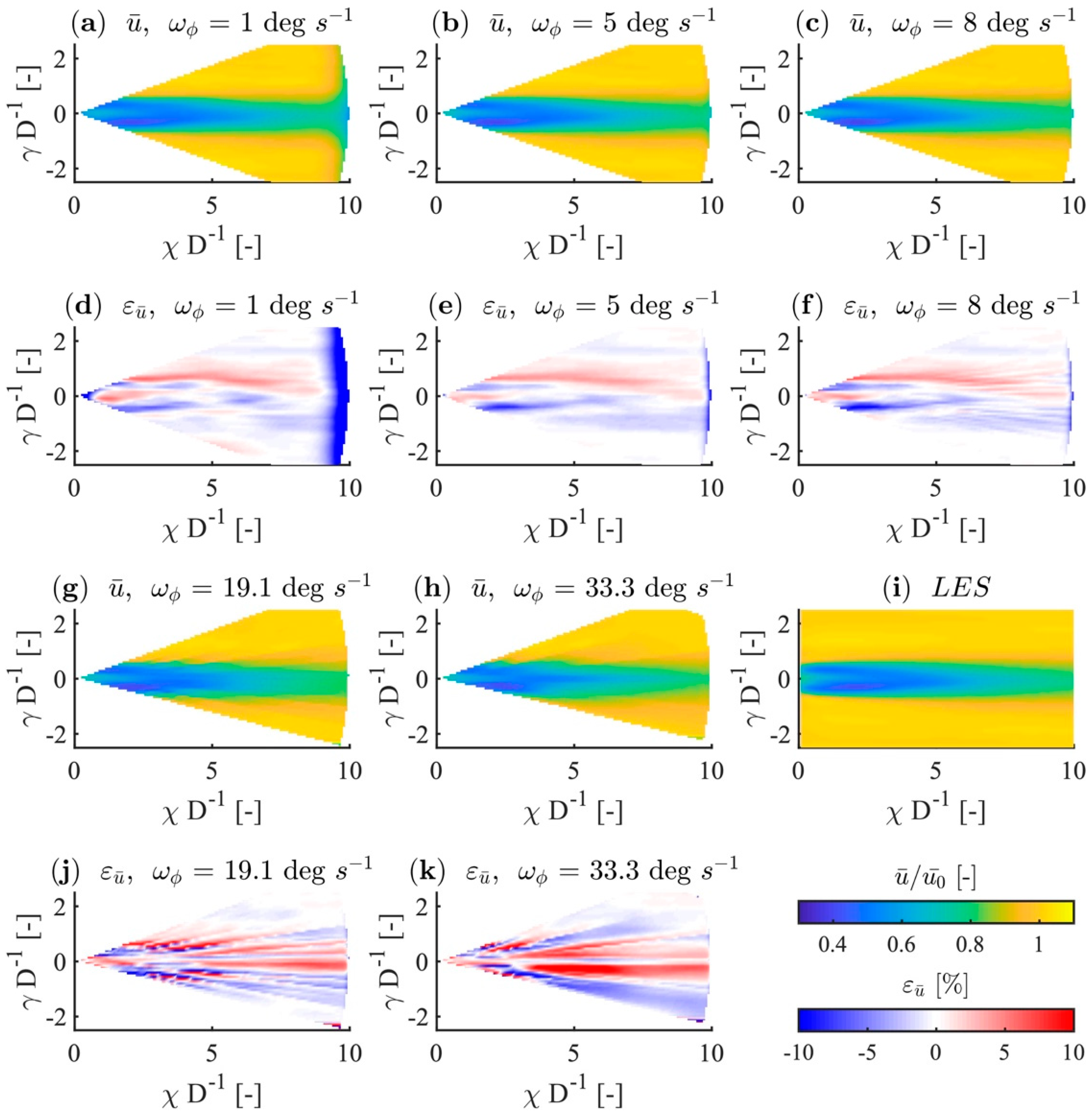
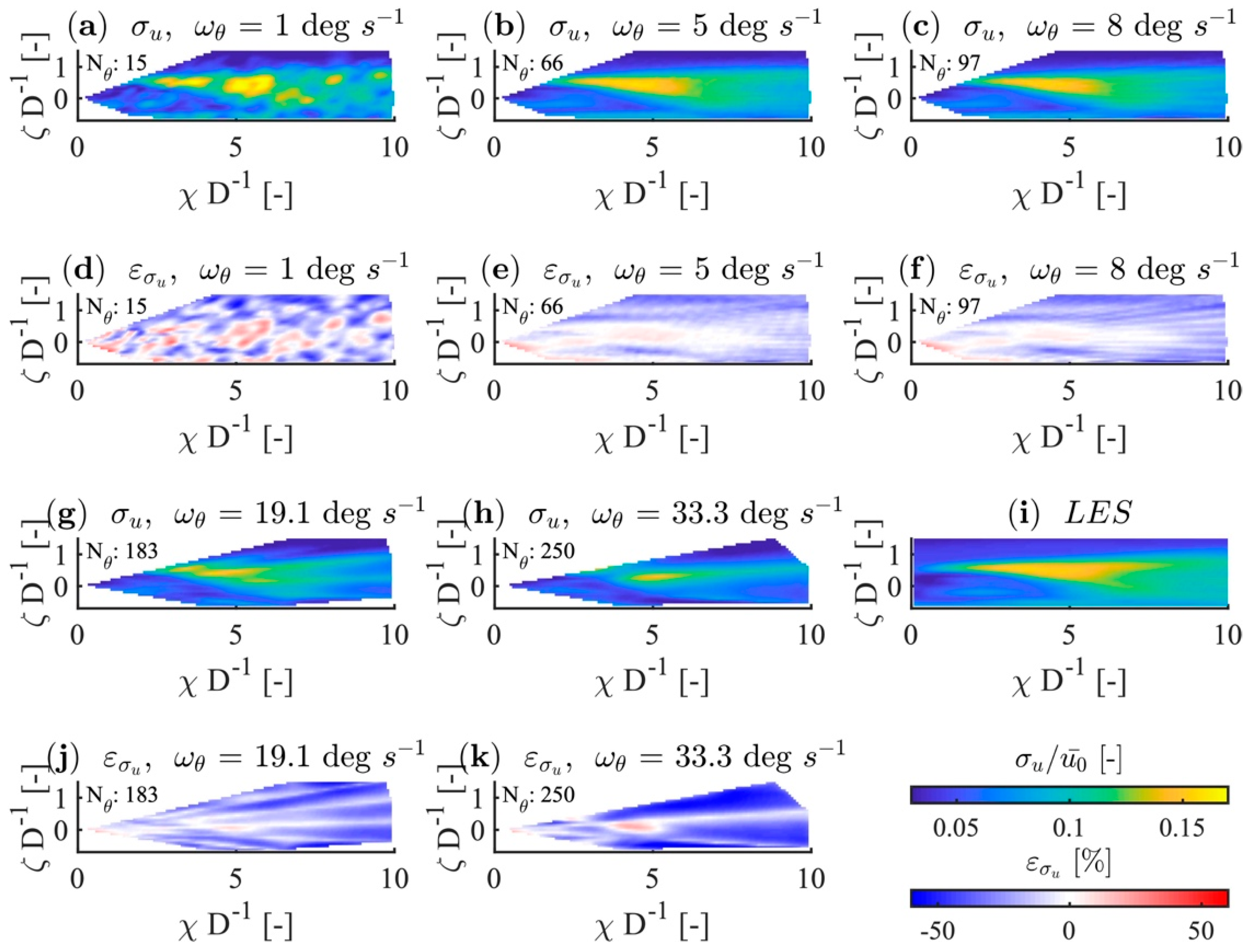
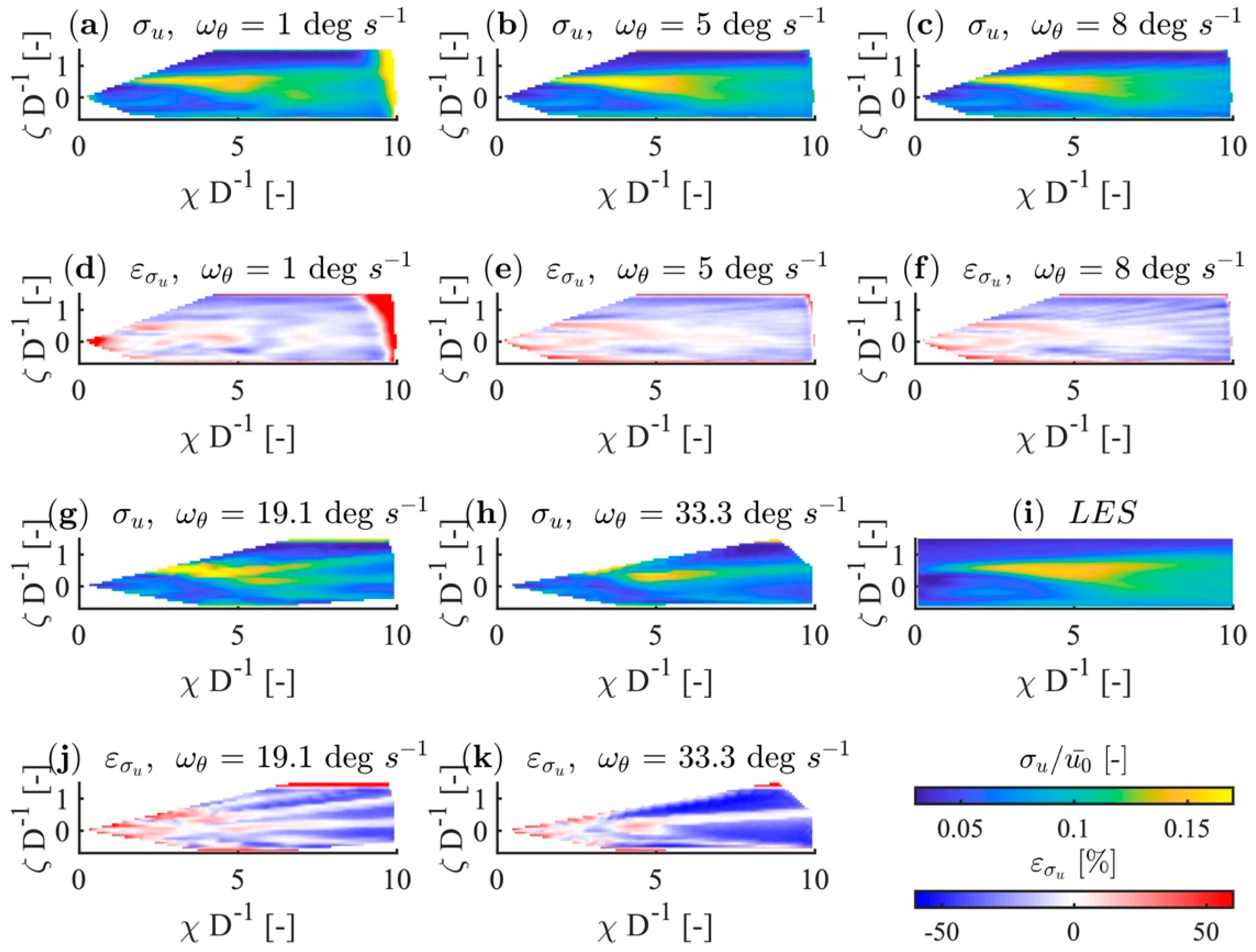
Slow scan speeds yield fine spatial and coarse temporal resolution and fast scan speeds give the opposite resolutions. These effects are shown in the visualisation of the 10-min averaged wind speeds shown in Figure 7 and the distribution of the standard deviations shown in Figure 8. The low temporal resolution is indicated by the wavy flow structures along the wake in the plot of average wind speeds in Figure 7a,b,d,e and in the standard deviations in Figure 8a,b,d,e. These features arise because the number of scans is not sufficient to form a smooth flow field, as stated in Equation (1). In contrast, structural artefacts of quantification by the laser beam along the wake can be seen in Figure 7c,f–h,j,k, which indicate that the spatial resolution is lower than the LES averages in Figure 7i. The strip-shaped structures in the standard deviation (Figure 8c,f–h,j,k) indicate the limits of the LIXIM LiDAR simulator, which does not reproduce volume-averaging behaviour in the scanning direction. The quantisation of the measurement area with single beams can be seen in the reduction of the standard deviation. Since no measurements are recorded between the individual laser beams, the standard deviation cannot be higher than it is directly on the beams due to the interpolation from inter-polar coordinates to the Cartesian grid. Thus, we see a transition from good spatial to good temporal resolution as the angular velocity changes from 1.00°/s to 33.33°/s. While the variation of the angular velocity apparently has a minor influence on the measurement of the structure of the average wake velocity, the expected under-estimation of the standard deviation caused by volume averaging and the measurement frequency ($f_s$) can be seen in the wake region as the angular velocity (${\omega }_{\varphi }$) increases (Figure 8g,h).

4.1.1. Error Case Discrimination

We determine the deviation from the LES by defining an average velocity error:

$${\epsilon }_{\overline{u}}=\frac{\overline{u_{lidar}}-\overline{u_{LES}}}{\overline{u_{LES}}},$$

(22)

and the standard-deviation error:

$${\epsilon }_{{\sigma }_u}=\frac{{\sigma }_{lidar}-{\sigma }_{LES}}{{\sigma }_{LES}},$$

(23)

where $N_{lidar}$ is the number of velocity points included in the original LiDAR data, while $N_{LES}$ is the number of corresponding velocity points in the LES data. Note that $u$ is normalised before this step, so that ${\epsilon }_{\overline{u}}$ and ${\epsilon }_{{\sigma }_u}$ are dimensionless and are given in percentages.

For a more detailed analysis, we distinguished three regions of errors:

• Error at the centreline in the wake: $\gamma D^{-1}=0$ and $\zeta D^{-1}=0$.
• Planar wake error: $-1\le \gamma D^{-1}\le 1$ and $-1\le \zeta D^{-1}\le 1$.
• Error in the free stream outside of the wake (opposite the planar wake case).

We introduce these three groups of errors to clarify the added volume-averaging error in the scanning direction. Since this effect is not reproduced in the LiDAR simulator, we attempted to account for it by posteriorly averaging the planar error. The aim of this process was not exactly to recreate the scan-wise volume averaging in the measured data, but instead to reproduce a similar trend. As a result, the first case, considering data on the centreline, reproduces the step-and-stare measurement behaviour. The second case, planar wake error, resembles the behaviour of on-the-fly measurements. The third case considers free-stream error in the measurements of flow outside of the wake.

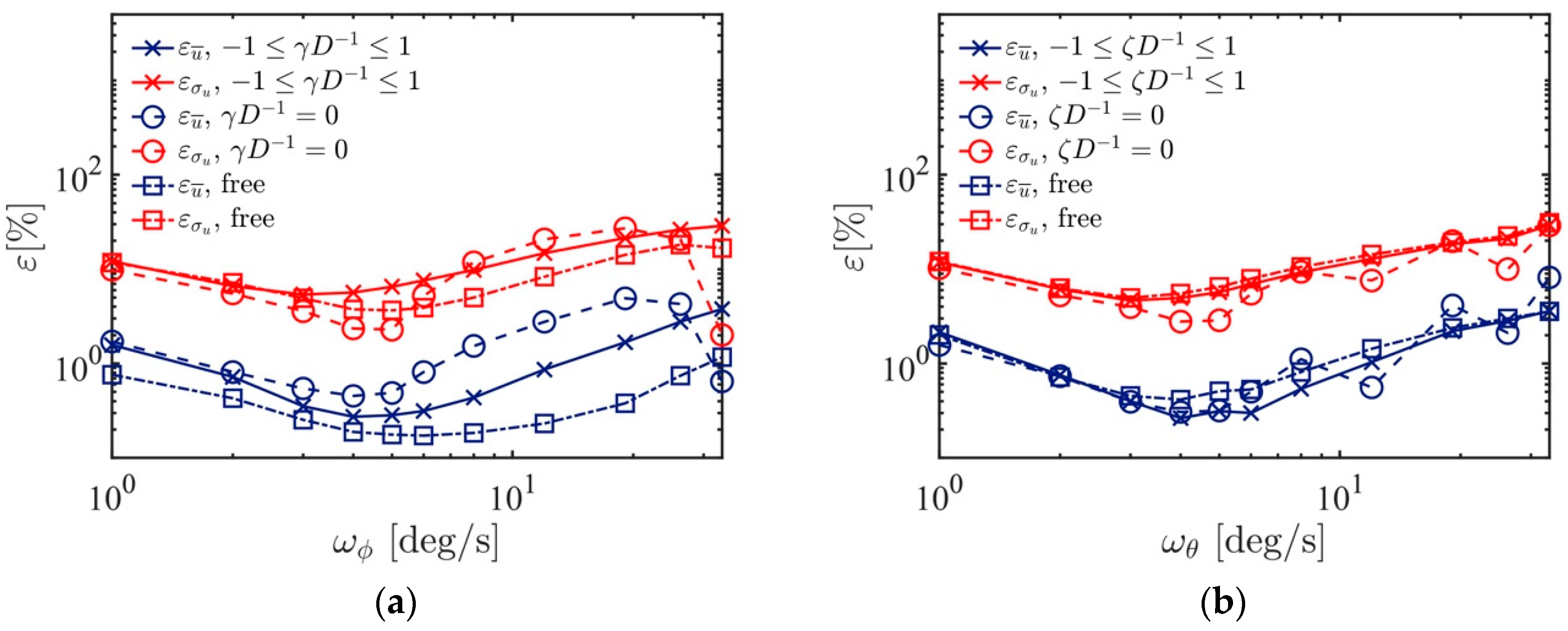
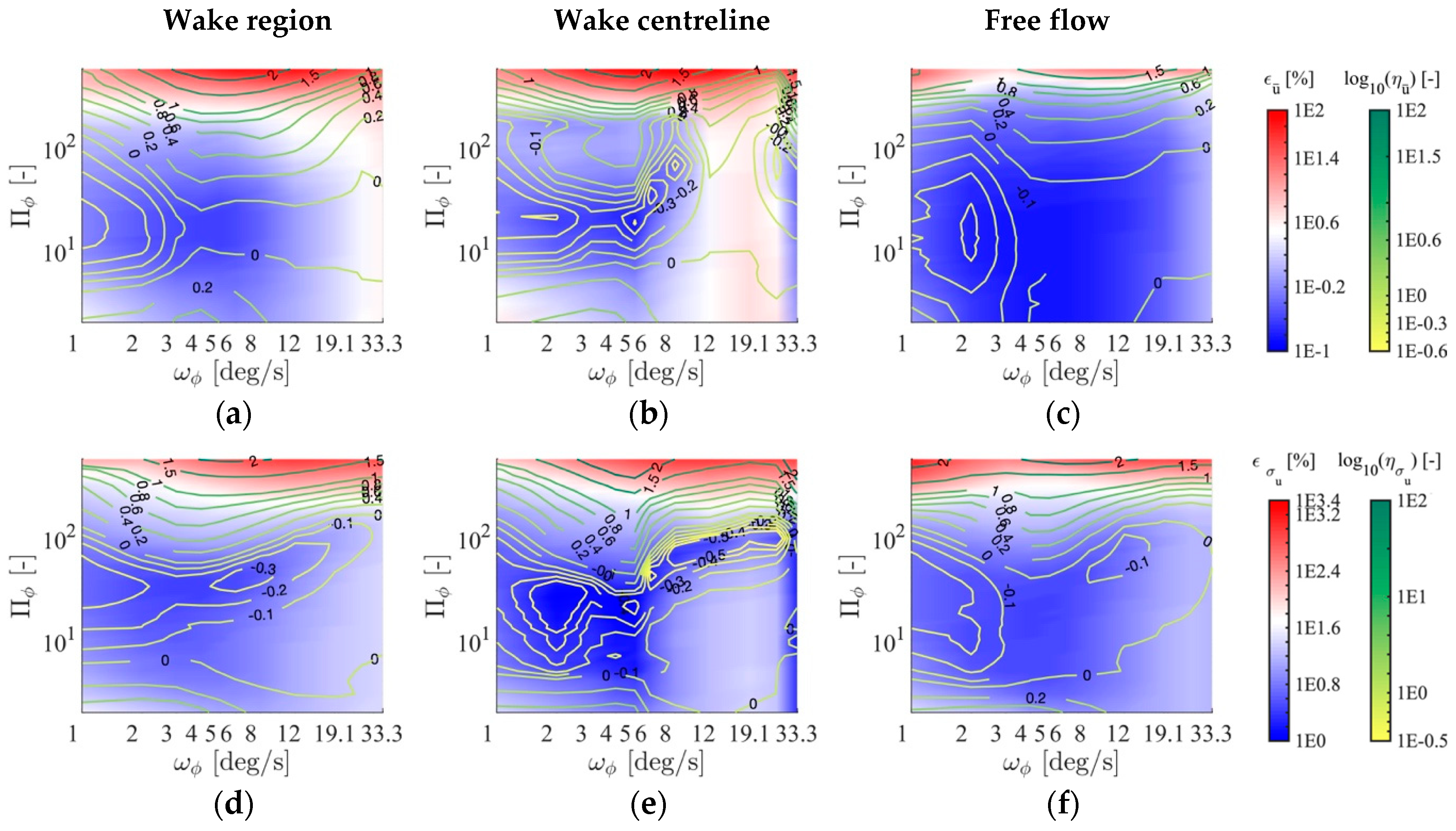
The plots in Figure 9 show the behaviour of ${\epsilon }_{\overline{u}}$ and ${\epsilon }_{{\sigma }_u}$ for each of the three types of error, depending on the scan speeds, ${\omega }_{\varphi }$ and ${\omega }_{\theta }$. As mentioned above in Section 1, the largest errors occur at the extremes of very slow and very fast measurements. In general, similar behaviour is seen in all the errors in the PPI and RHI measurements. The errors are high at the scanning speed of 1°/s, decrease as the scan speed increases until the minima are reached, and increase again up to the speed of 33.33°/s.

Mean-value error (${\epsilon }_{\overline{u}}$) and the standard-deviation error (${\epsilon }_{{\sigma }_u}$) emerge along the centreline in the RHI scans, $\zeta D^{-1}=0$. At the scanning speed of ${\omega }_{\theta }=8°/\mathrm{s}$, these errors are more scattered than the other errors. In addition, the centreline errors in the PPI scans show an unexpectedly low value at the scanning speed of ${\omega }_{\varphi }=33.33°/\mathrm{s}$, which we are unable to explain. The wind-speed data along the centreline is clearly affected the least by the change between the polar and Cartesian coordinate systems, since the scan geometry and the resulting distribution of angular measurements cover this line more consistently than other positions with measurement points. While all errors in the RHI and PPI scans decrease along with increasing angular speeds, the ensemble minimum occurs at approximately 5°/s. The centreline error increases dramatically after 5°/s. The logarithmic representation in these plots makes it difficult to recognise the point symmetry of the error behaviour. The PPI error is symmetric around the minimum at ${\omega }_{\varphi }=4°/\mathrm{s}$ and ${\epsilon }_{\overline{u}}$ = 0.46 %. The minimum of the standard deviation is found at ${\omega }_{\varphi }=5°/\mathrm{s}$ and ${\epsilon }_{{\sigma }_u}=$2.29 %. In the RHI scans, errors of the same magnitude are seen at ${\omega }_{\theta }=4°/\mathrm{s}$ with ${\epsilon }_{\overline{u}}=0.31\%$ and at ${\omega }_{\theta }=4°/\mathrm{s}$ with ${\epsilon }_{{\sigma }_u}=2.78\%$.

By averaging all points in the wake,$-1\le \gamma D^{-1}\le 1$ and $-1\le \zeta D^{-1}\le 1$, the representation of wind speed with the LiDAR measurements is improved. The average wind-speed error (${\epsilon }_{\overline{u}}$) is smaller than the centreline error in the PPI and RHI scans. However, since the standard-deviation error (${\epsilon }_{{\sigma }_u}$) is more pronounced than the mean wind-speed error (${\epsilon }_{\overline{u}}$), we conclude that volume averaging of the LiDAR measurements and the associated time shift within the scans accurately reproduces the mean wind speed, although the measured values are widely dispersed. In this case, the minimal error of the standard deviation is ${\epsilon }_{{\sigma }_u}=$5.40 % at ${\omega }_{\varphi }=3°/\mathrm{s}$ for the PPI scans and ${\epsilon }_{{\sigma }_u}=$4.98 % at ${\omega }_{\theta }=3°/\mathrm{s}$ for the RHI scans. This minimum indicates that the local turbulence intensity averaged over the wake can be reproduced with an accuracy of ~5 % in absolute terms.

As expected, the free-flow errors for the PPI scan are the lowest of any in our analysis. Since the RHI scans mainly map the wake due to the scan geometry (Figure 9), free flow could not be defined exactly. These values are given for completeness, but should not be used for drawing generalised conclusions. The PPI free-stream error shows similar behaviour to that of the averaged wake errors, which is likely due to the process of area averaging. The errors are scaled over the scan speeds towards lower values. The minimum of ${\epsilon }_{\overline{u}}=$0.17% occurs at ${\omega }_{\varphi }=6°/\mathrm{s}$, and the minimum of ${\epsilon }_{{\sigma }_u}=$3.68% occurs at ${\omega }_{\varphi }=5°/\mathrm{s}$, which are comparable to the centreline errors. Since the turbulence intensity increases considerably compared to the ambient conditions in the high-shear areas of the wakes (Figure 8i), we deduce that, with lower turbulence intensities, the mapping error is minimal so the optimal scanning speed is faster. This relationship means that the more a flow fluctuates, measuring spatial structure becomes more important than measuring temporal changes.

The data corresponding to Figure 9 is listed in

Table A1. Average wind speed and standard deviation error against the LES of PPI scans for different angular velocities, ${\omega }_{\varphi }$.

	1°/s	2°/s	3°/s	4°/s	5°/s	6°/s	8°/s	12°/s	19.1°/s	27.2°/s	33.3°/s
wake region$\mathbf{-}\mathbf{1}\mathbf{\le }\mathit{\gamma }{\mathit{D}}^{\mathbf{-}\mathbf{1}}\mathbf{\le }\mathbf{1}$
${\mathit{\epsilon }}_{\overline{\mathit{u}}}$	1.68%	0.72%	0.36%	0.29%	0.31%	0.35%	0.49%	0.99%	1.99%	3.17%	4.21%
${\mathit{\epsilon }}_{{\mathit{\sigma }}_{\mathit{u}}}$	12.61%	5.71%	4.81%	5.00%	5.93%	7.06%	9.43%	14.83%	21.04%	25.63%	27.85%
wake centreline$\mathit{\gamma }{\mathit{D}}^{\mathbf{-}\mathbf{1}}\mathbf{=}\mathbf{0}$
${\mathit{\epsilon }}_{\overline{\mathit{u}}}$	1.71%	0.81%	0.54%	0.46%	0.49%	0.81%	1.54%	2.77%	4.91%	4.27%	0.65%
${\mathit{\epsilon }}_{{\mathit{\sigma }}_{\mathit{u}}}$	9.81%	5.54%	3.59%	2.36%	2.29%	5.23%	11.87%	20.65%	27.09%	20.72%	2.01%
free flow
${\mathit{\epsilon }}_{\overline{\mathit{u}}}$	0.77%	0.43%	0.25%	0.19%	0.18%	0.17%	0.18%	0.23%	0.38%	0.74%	1.17%
${\mathit{\epsilon }}_{{\mathit{\sigma }}_{\mathit{u}}}$	11.78%	7.19%	4.91%	3.77%	3.68%	3.90%	5.00%	8.34%	14.22%	18.15%	16.69%

and

Table A2. Average wind speed and standard deviation error against the LES of RHI scans for different angular velocities, ${\omega }_{\theta }$.

	1°/s	2°/s	3°/s	4°/s	5°/s	6°/s	8°/s	12°/s	19.1°/s	27.2°/s	33.3°/s
wake region$\mathbf{-}\mathbf{1}\mathbf{\le }\mathit{\zeta }{\mathit{D}}^{\mathbf{-}\mathbf{1}}\mathbf{\le }\mathbf{1}$
${\mathit{\epsilon }}_{\overline{\mathit{u}}}$	2.15%	0.76%	0.40%	0.26%	0.31%	0.30%	0.54%	1.04%	2.21%	2.84%	3.59%
${\mathit{\epsilon }}_{{\mathit{\sigma }}_{\mathit{u}}}$	11.87%	6.15%	4.66%	4.96%	5.70%	6.94%	9.24%	12.87%	18.43%	21.02%	29.30%
wake centreline$\mathit{\zeta }{\mathit{D}}^{\mathbf{-}\mathbf{1}}\mathbf{=}\mathbf{0}$
${\mathit{\epsilon }}_{\overline{\mathit{u}}}$	1.58%	0.73%	0.39%	0.31%	0.32%	0.50%	1.11%	0.56%	4.13%	2.11%	8.20%
${\mathit{\epsilon }}_{{\mathit{\sigma }}_{\mathit{u}}}$	10.28%	5.29%	3.97%	2.78%	2.87%	5.47%	9.37%	7.58%	19.78%	10.00%	28.98%
free flow
${\mathit{\epsilon }}_{\overline{\mathit{u}}}$	2.01%	0.72%	0.45%	0.42%	0.51%	0.53%	0.81%	1.44%	2.39%	3.00%	3.58%
${\mathit{\epsilon }}_{{\mathit{\sigma }}_{\mathit{u}}}$	12.02%	6.27%	4.98%	5.51%	6.48%	7.92%	10.60%	14.26%	19.26%	22.48%	30.87%

in Appendix B.

4.2. Time-Resolution Improvement

To evaluate the effects of increasing the temporal resolution of the synthetic LiDAR data, we first propagated the LiDAR scan backwards and forwards using the wind-field propagation method described in Section 3.2 to obtain a mixed and closed space-time conversion. Then, we compared the propagated scans with the reference LES wind field. We corrected the scan-containing time error and synchronised the propagated data with the LES time data. In this subsection, we first discuss the effect of the propagation on the temporally averaged values, like the mean value and the standard deviation, before we address the dynamic behaviour. The following results are based on the averages of the optimal time steps achieved in Section 4.3. For the results herein, we used ${\mathsf{\Pi }}_{\varphi }=16$ as the number of interpolation steps for the PPI data and ${\mathsf{\Pi }}_{\varphi }=14$ for the RHI data. The influence of ${\mathsf{\Pi }}_{\varphi ,\theta }$ is discussed in Section 4.3. We present all the RHI-related results in Appendix C.

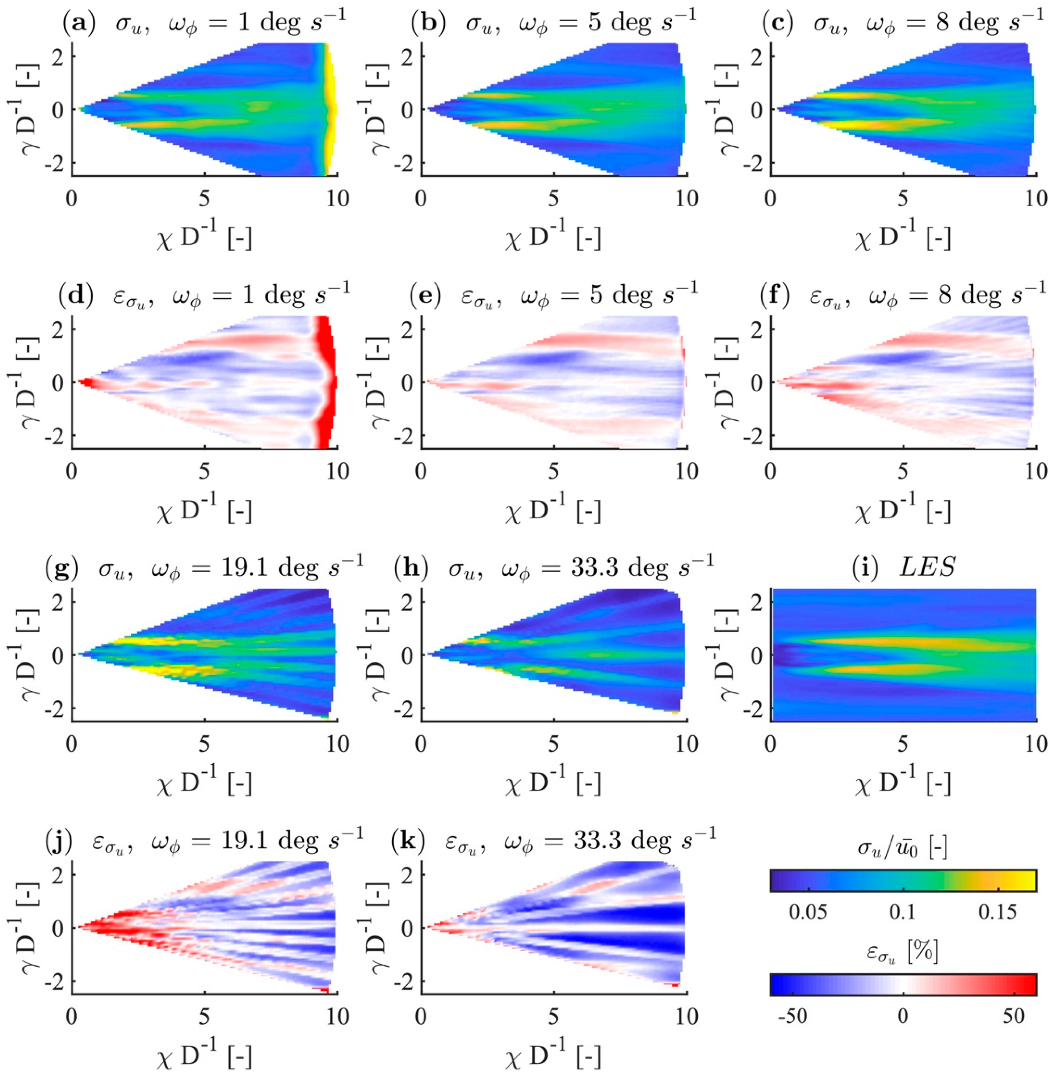
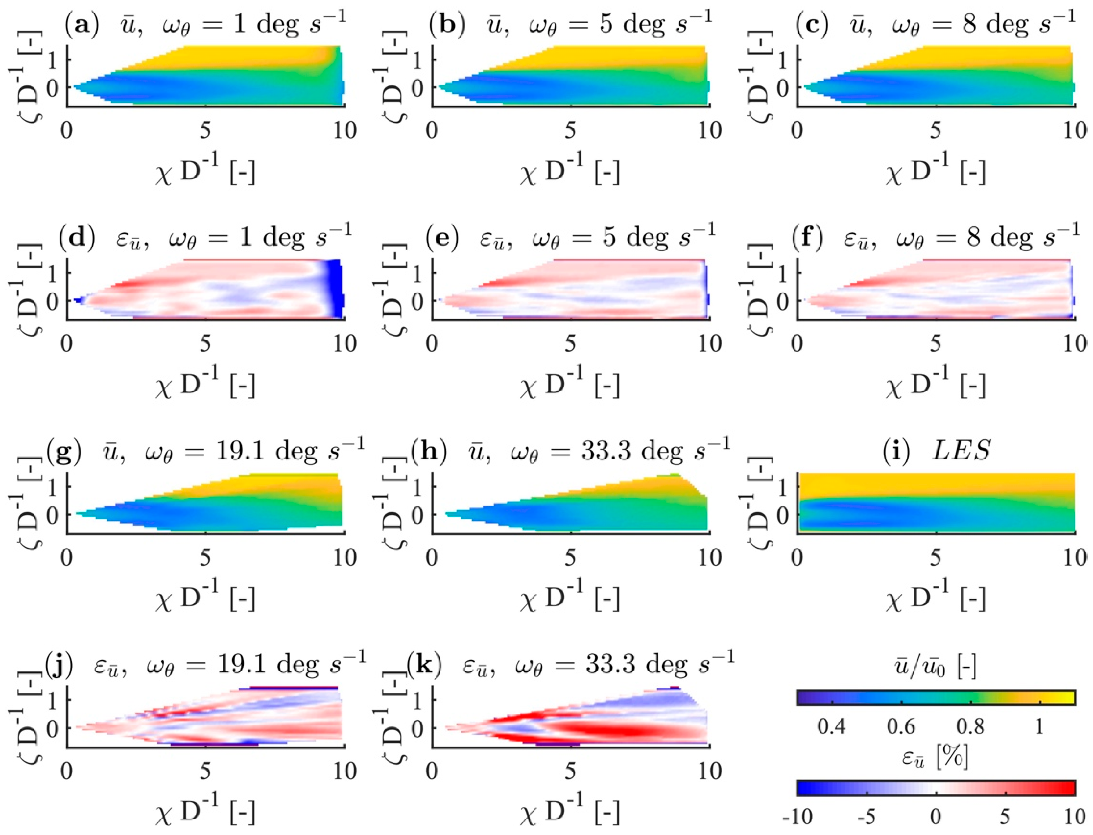
Figure 10 illustrates the averaged wind speed ($\overline{u}$) of the propagated PPI data, which are analogous to the original PPI data shown in Figure 7. As with the original LiDAR scan discussed in Section 4.1, no significant differences in the mean wind speeds of the wake appear. When considering the differences from the LES data (Figure 10d–f,j,k and Figure 11d–f,j,k), the same deviation structures occur independently of the angular velocity, even though the structures become coarser because of angular quantisation at faster sampling rates. Compared with Figure 7a,b,d,e, in which individual flow artefacts that are caused by the very low number of samples appear, the artefacts in the propagated data in Figure 10a,b,d,e are smoothed into the flow direction and are much more like the LES reference data. With propagation and synchronisation with the LES time steps, the number of scans is increased by a factor of 2.4 to 40 within the 10-min time period. Depending on the scanning speed, the structural representation of the flow field is significantly improved.

For the angular velocities, ${\omega }_{\varphi }=1°/\mathrm{s}$ and ${\omega }_{\varphi }=5°/\mathrm{s}$(Figure 10a,b,d,e), propagation artefacts are clearly visible at the extremes of the measurement domain around $\mathsf{\chi }{D}^{-1}$ = 10. In those cases, the interpolation time (${\mathrm{T}}_{\varphi }$) and the propagation domain create a mixture of wind speeds with boundary conditions in combination with the mean flow velocity, and this blending manifests as a reduction of wind speed. These artefacts can also be seen in the visualisation of the standard deviation of the wind speed shown in Figure 11a,b,d,e, which are no longer detectable if ${\omega }_{\varphi }>5°/\mathrm{s}$.

The effect of the quantisation of the measurement area by individual angular measurements, which is also remarked upon in Section 4.1 and Section 4.3, is not compensated for by wind-field propagation and is still visible if ${\omega }_{\varphi }\ge 8°/\mathrm{s}$ (Figure 11c,f–h,j,k).

To address the dynamic effects of wind-field propagation and to reveal a holistic understanding of the dynamic behaviour, the reader should refer to the supplementary information of video S1 for horizontal slices and video S2 for vertical slices. Videos S1 and S2 show the main wind-speed components ($u$) of the propagated LiDAR data and deviations from the LES reference for different angular velocities, which are analogous to the data in Figure 7. As the angular velocity increases, flow structures are represented with decreasing accuracy because of the decreasing point density of the polar grid. Artefacts due to inconsistent advection velocities during the propagation between two scans can be detected in the errors (${\epsilon }_u$) oriented in the flow direction. These artefacts are most evident at the midpoint between two laser-beam passes (red line) and below the laser beam. In addition, the effect of mixing the boundary conditions with the measured wind speeds appears below the laser beam.

Because of the interpolation method visualised in Figure 5, the instantaneous wind-speed error (${\epsilon }_u=\frac{u_{\mathrm{propagated}}-u_{\mathrm{LES}}}{u_{\mathrm{LES}}}$) is lowest around the position of the moving laser beam, since the wind speed in this region corresponds to the un-propagated LiDAR data. The resulting error in the immediate surroundings of the laser beam indicates the volume-averaging error in the beam direction.

4.3. Influence of the Interpolation Time Step, Δt, on the Statistical Error

As we discussed in Section 3.3, the number of propagation steps ($\mathsf{\Pi }$) between two measured scans influences the temporal accuracy of the mapping of a scan interpolated at a certain time (t). If $\mathsf{\Pi }$ is too low, the temporal changes in the flow structures are not resolved sufficiently, which increases the temporal error. Since our interpolation method employs a simplistic approach to represent fluid dynamics, the propagation will make the representation diverge somewhat from a realistic physical picture of the flow field. As more steps are interpolated between two scans, the temporal aspect of the reproduction of the flow between each scan will improve. At the same time, the reconstruction error will increase. Since some inaccuracy will arise in the speed of advection between pairs of scans, the position of the flow structures will be shifted somewhat. To investigate the effects of different interpolation steps ($\mathsf{\Delta }t$) and to determine the parameter configuration that has the lowest statistical errors, we have evaluated different values of $\mathsf{\Pi }$ for each scanning speed, ${\omega }_{\varphi ,\mathsf{\theta }}$. The corresponding results for RHI scans are presented in Appendix D.

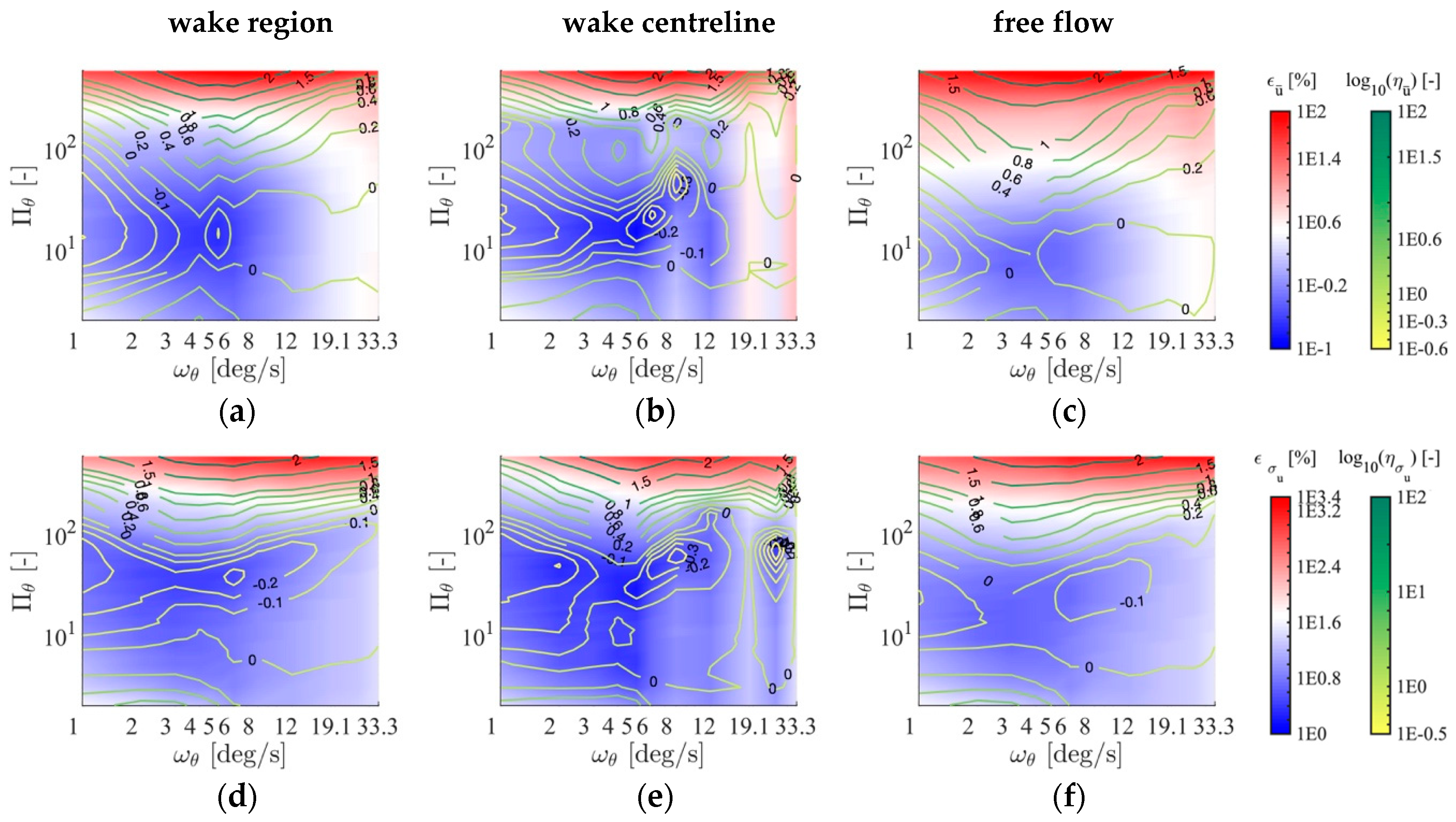
Applying the definition of the averaged error (${\epsilon }_{\overline{u}}$) in Equation (22) and the standard-deviation error, ${\epsilon }_{{\sigma }_u}$, in Equation (23) to the temporally improved wind fields with different combinations of ${\omega }_{\varphi }$ and ${\mathsf{\Pi }}_{\varphi }$ (respectively, ${\omega }_{\mathsf{\theta }}$ and ${\mathsf{\Pi }}_{\mathsf{\theta }}$), Figure 12 shows the resulting three error cases that were reduced above:

• Inside the wake for $-1\le \gamma D^{-1}\le 1$ and $-1\le \zeta D^{-1}\le 1$.
• Along the centreline for $\gamma D^{-1}=0$ and $\zeta D^{-1}=0$.
• In the free flow.

The errors are shown in colour, and the iso-lines represent the power of the ratio of the error of the propagated data to the error of the original LiDAR data, ${\eta }_{\overline{u}}=\frac{{\epsilon }_{\overline{u}}{}_{propagated}}{{\epsilon }_{\overline{u}}{}_{lidar}}$ and ${\eta }_{{\sigma }_u}=\frac{{\epsilon }_{{\sigma }_u}{}_{propagated}}{{\epsilon }_{{\sigma }_u}{}_{lidar}}$.

For the sake of readability, we have listed the configurations that give minimum errors in

Table 2. Combinations of $\omega$ and $\mathsf{\Pi }$ that give local minima for different error regions in the PPI and RHI data.

	PPI			RHI
	Wake Region	Wake Centreline	Free Flow	Wake Region	Wake Centreline	Free Flow
$\omega$	5°/s	5°/s	5°/s	5°/s	5°/s	3°/s
$\mathsf{\Pi }$	16	18	9	14	16	7
${\mathit{\epsilon }}_{\overline{\mathit{u}}}$	0.24%	0.15%	0.14%	0.20%	0.13%	0.40%
$\omega$	4°/s	5°/s	4°/s	4°/s	5°/s	3°/s
$\mathsf{\Pi }$	33	21	16	33	26	13
${\mathit{\epsilon }}_{{\mathit{\sigma }}_{\mathit{u}}}$	2.89%	0.60%	3.02%	2.79%	1.61%	4.53%

.

The results in Figure 12 show that an optimal interpolation time step exists for each angular velocity. If we compare these results with those in Figure 9, we see that a single optimal angular velocity yields the smallest mapping errors for a set of wake speed and atmospheric conditions. The resulting ${\eta }_{\overline{u}}$ and ${\eta }_{{\sigma }_u}$ are plotted as iso-lines in Figure 12 to show which value of ${\mathsf{\Pi }}_{\varphi }$ most improves the temporal resolution and minimises the absolute error. These values show the exponent of the decimal expression of ${\eta }_{\overline{u}}$ and ${\eta }_{{\sigma }_u}$. The zero line is a significant feature as it indicates the boundary at which the combination of ${\omega }_{\varphi }$ and ${\mathsf{\Pi }}_{\varphi }$ shifts from reducing to amplifying the mapping error. In all three regions, both the average wind-speed error and standard-deviation error are reduced over the entire range of angular velocities. The most significant improvements are achieved at scanning speeds slower than the optimum, but they do not reflect the absolute smallest error. The results in Figure 12 show that for the test case we considered, the error is reduced to the minimum of ${\eta }_{\overline{u}}$ = 30.5% of the original ${\epsilon }_{\overline{u}}$ and to ${\eta }_{{\sigma }_u}$ = 42% of the original ${\epsilon }_{{\sigma }_u}$. The most significant improvements are outlined in

Table 3. Combinations of $\omega$ and $\mathsf{\Pi }$ that optimize ${\eta }_{\overline{u}}$ and ${\eta }_{{\sigma }_u}$ for different cases of PPI and RHI data.

	PPI			RHI
	Wake Region	Wake Centreline	Free Flow	Wake Region	Wake Centreline	Free Flow
$\omega$	1°/s	2°/s	2°/s	1°/s	1°/s	1°/s
$\mathsf{\Pi }$	16	21	13	13	16	8
${\eta }_{\overline{u}}$	35.5%	31.0%	36.9%	30.5%	31.2%	46.5%
$\omega$	1°/s	1°/s	1°/s	1°/s	1°/s	1°/s
$\mathsf{\Pi }$	33	42	37	67	60	26
${\eta }_{{\sigma }_u}$	42.8%	43.6%	45.6%	43.9%	42.0%	60.5%

.

5. Discussion

Scanning LiDAR measurements must strike a compromise between temporal and spatial resolution. Since full-field measurements are usually very expensive, the scan parameters are usually chosen to minimize the scanning time. The greatest obstacle to the choice of effective scanning parameters is the limited availability of adequate validation measurements, so we used synthetic LiDAR data to verify the validity of parameter choices. This synthetic dataset raises questions about transferability and the extent to which the combination of a synthetic wind field and a LiDAR simulator can represent realistic characteristics of full-field LiDAR measurements. As discussed in Section 2.2, the lack of volume averaging in the scanning direction limits the direct transferability of synthetic data to step-and-stare LiDAR measurements. In most actual cases [21,26,33,43,46,47,48,49,50,51], scanning measurements are taken on-the-fly to minimize the scanning time. This tendency implies that during the angular movement of the scanner head, backscattering is accumulated continuously, so the velocity measurements are averaged over the traversed volume of air. Real on-the-fly measurements will show a higher reduction in the standard deviation caused by this additional averaging. Though the data processing within a LiDAR system can be regarded as a non-linear signal process, we compensated for the effects of scanning-volume averaging with retrospective averaging. We considered this missing effect with a separate consideration of the mean and standard-deviation error at the centreline to representing the on-beam behaviour and planar error.

Optics and internal signal processing are also not considered in the LiDAR simulator, as described by Stawiarski et al. [34]. The calculated velocities have the typical device characteristics of one-dimensionality and beam-wise volume averaging, but no indication of the measurement quality, which is usually given by the carrier-to-noise ratio (CNR) or signal-to-noise ratio (SNR). In a real device, the variations in the CNR or SNR and the resulting fluctuations in the wind speed after filtering tend to reduce the data availability [26], which is also not reproduced in the simulation. The test case discussed above therefore represents an idealisation of the measurements in every respect, so it naturally draws attention to the peculiarities of real LiDAR measurements.

The results given above are based on the projection of the LOS velocities in the main wind direction that was described in Section 3.1. The assumption of homogeneity in the projection affects the accuracy of the representation of the wind-speed statistics, especially in areas where the assumption does not apply (in the near-wake region ($\mathsf{\chi }{D}^{-1}\le 3$)). Further, the calculation of the standard deviation from the projected time series of LOS velocities introduces some error due to the non-linear dependency of the standard deviation of the LOS velocities (${\sigma }_{{\widehat{\upsilon }}_{LOS}})$ on the standard deviations of the main wind-speed components (${\sigma }_u$, ${\sigma }_v$, ${\sigma }_w$). From Figure 8 and Figure 11, one can see that the error in the standard deviation from deviations in the measurement angle (${\varphi }^{\prime }\ne 0$ and ${\theta }^{\prime }\ne 0$) in the main flow direction is marginal compared to the error of the standard deviation due to the spatial and temporal quantisation. Otherwise, a clear trend in the error versus the measuring angle would be apparent in Figure 8 and Figure 11. This statement only applies to the present test case since the difference in the angles of the measurement and the main wind direction (${\varphi }^{\prime },{\theta }^{\prime }$) are very small because of the nacelle-based measurement setup. We are aware that the projection error increases with increasing ${\varphi }^{\prime }$ and ${\theta }^{\prime }$, but we cannot isolate this effect within the scope of this paper. We do assume that this source of error will have more of an effect if the scanned area is not aligned with the main wind direction, which is confirmed in Fuertes and Porté-Agel [27] for ground-based measurements.

For these reasons, we cannot claim that transfer to real data will results in the same degree of improvement in the mapping accuracy. The basis of data with which this study was conducted is too limited. To consider the general transferability of the propagation method discussed above, more flow situations with variable atmospheric conditions will need to be investigated analogously. These could be combined into a database that would give optimal measurement parameters for a range of atmospheric conditions.

When improving temporal resolution, the space-time conversion proposed above will introduce some error. The results in Section 4.3 indicate that this numerical error increases along with the number of interpolations and will produce the minimal mapping error with some combinations of scan parameters. In the present study, we were not able to determine the extent to which the improvement in the mapping accuracy is due to the statistical correlation described in Equation (1).

Regardless of the requirement of statistical independence imposed by Equation (1), we saw an improvement in the mapping quality of the mean values. The improvement in the standard deviation should be considered more critically and will be analysed again in a future study. A reasonable approach might consider, first, the ratio of the LiDAR accumulation time to the temporal resolution of the LES and, second, the nature of the step-and-stare measurement method. Further studies should evaluate the extent to which improvements to the standard deviation achieved with the wind-field propagation method satisfy turbulence characteristics, or whether this improvement is merely coincidental.

6. Conclusions

This paper has presented a space-time conversion method for long-range planar LiDAR data, which achieves temporal interpolation that reflects reasonable approximations of fluid-dynamic processes. This method allowed us to retrospectively improve the temporal resolution of successive scans and to synchronise the scans with measurements collected with different time stamps. This method corrects for time shifts within a scan by applying a sinusoidal weighted average of forward- and backward-propagated wind fields taken from different completed scans, which fills in the unmeasured flow behaviour. We used synthetic LiDAR data generated by a numerical simulator and in an LES wind-turbine wake flow field to evaluate the method in terms of the mean wind speed and standard deviation.

A parametric study of 11 scanning velocities for both PPI and RHI scans was then carried out for a test case with an ambient wind speed of $u_0=8\mathrm{m}/\mathrm{s}$ and a turbulence intensity of $I_0=5.8\%$. Using a total of 2334 scans, we revealed how the mapping error in the LiDAR measurements is affected by the angular-scan velocity. This error is temporal in nature at low scanning speeds and shifts to a spatial error at high scanning speeds. The optimal scanning speed is determined by the turbulence intensity and the corresponding spatial variability in the wind-turbine wake. Analysis of 11 different scan velocities showed that, with the careful selection of typical measurement parameters, the compromise between temporal and spatial resolution is well balanced. In the specific test case we considered, the optimal measurements are taken with slower scan speeds and higher spatial resolutions. The use of wind-field propagation increased the volume of synthetic LiDAR data by a factor of 2.4 to 40, allowing synchronisation with the LES reference data. This synchronization led to an improvement of the structural mapping, in terms of both the mean wind speed and the standard deviation.

The interpolation method can be used with various configurations of interpolation steps between two scans, so it can serve as a universal tool for increasing the temporal resolution of planar LiDAR measurements with a minimal increase in statistical errors. This interpolation is particularly useful for the analysis and comparison of wake measurements, for which some wake characteristics might be correlated with data of finer temporal resolution recorded external to the wind turbine, such as load data. In addition to synchronising the data from complex measurement campaigns taken with various LiDAR devices and sensors, the possibility of temporal up-sampling allows for easier processing. In the test case discussed above, the maximum reduction of the error of the mean wind speed was 30.5% and the standard-deviation error was reduced by 42%.

References

- Crespo, A.; Hernández, J.; Frandsen, S. Survey of modelling methods for wind turbine wakes and wind farms. Wind Energy 1999, 2, 1–24. [Google Scholar] [CrossRef]
- Vermeer, L.J.; Sørensen, J.N.; Crespo, A. Wind turbine wake aerodynamics. Prog. Aerosp. Sci. 2003, 39, 467–510. [Google Scholar] [CrossRef]
- Kelley, N.; Osgood, R.; Bialasiewicz, J.; Jakubowski, A. Using wavelet analysis to assess turbulence/rotor interactions. Wind Energy 2000, 3, 121–134. [Google Scholar] [CrossRef]
- Hand, M. Mitigation of Wind Turbine/Vortex Interaction Using Disturbance Accommodating Control. Ph.D. Thesis, National Renewable Energy Lab., Golden, CO, USA, 2003. [Google Scholar] [CrossRef] [Green Version]
- Manwell, J.F.; McGowan, J.G.; Rogers, A.L. Wind Energy Explained: Theory, Design and Application; John Wiley & Sons: Hoboken, NJ, USA, 2010. [Google Scholar]
- Ainslie, J.F. Calculating the flow field in the wake of wind turbines. J. Wind Eng. Ind. Aerodyn. 1988, 27, 213–224. [Google Scholar] [CrossRef]
- Jensen, N.O. A Note on Wind Generator Interaction Tech. Rep. Risø-M-2411(EN); Risø National Laboratory: Roskilde, Denmark, 1983. [Google Scholar]
- Frandsen, S.; Barthelmie, R.; Pryor, S.; Rathmann, O.; Larsen, S.; Højstrup, J.; Thøgersen, M. Analytical modelling of wind speed deficit in large offshore wind farms. Wind Energy 2006, 9, 39–53. [Google Scholar] [CrossRef]
- Larsen, G.; Madsen, H.; Thomsen, K.; Larsen, T. Wake meandering: A pragmatic approach. Wind Energy 2008, 11, 377–395. [Google Scholar] [CrossRef]
- Larsen, T.; Madsen, H.; Larsen, G.; Hansen, K.S. Validation of the dynamic wake meander model for loads and power production in the Egmond aan Zee wind farm. Wind Energy 2013, 16, 605–624. [Google Scholar] [CrossRef]
- Churchfield, M.J.; Lee, S.; Moriarty, P.J.; Hao, Y.; Lackner, M.A.; Barthelmie, R.; Lundquist, J.; Oxley, G. A Comparison of the Dynamic Wake Meandering Model, Large-Eddy Simulation, and Field Data at the Egmond aan Zee Offshore Wind Plant. In Proceedings of the 33rd Wind Energy Symposium 2015, Kissimmee, FL, USA, 5–9 January 2015. [Google Scholar] [CrossRef]
- Keck, R.-E.; de Maré, M.; Churchfield, M.J.; Lee, S.; Larsen, G.; Aagaard Madsen, H. On atmospheric stability in the dynamic wake meandering model. Wind Energy 2014, 17, 1689–1710. [Google Scholar] [CrossRef]
- Cheynet, E.; Jakobsen, J.B.; Snæbjörnsson, J.; Angelou, N.; Mikkelsen, T.; Sjöholm, M.; Svardal, B. Full-scale observation of the flow downstream of a suspension bridge deck. J. Wind Eng. Ind. Aerodyn. 2017, 171, 261–272. [Google Scholar] [CrossRef]
- Trabucchi, D.; Trujillo, J.J.; Schneemann, J.; Bitter, M.; Kühn, M. Application of staring LiDARs to study the dynamics of wind turbine wakes. Meteorol. Z. 2015, 6, 557–564. [Google Scholar] [CrossRef]
- van Dooren, M.F.; Campagnolo, F.; Sjöholm, M.; Angelou, N.; Mikkelsen, T.; Floris, M. Demonstration and uncertainty analysis of synchronised scanning LiDAR measurements of 2-D velocity fields in a boundary-layer wind tunnel. Wind Energy Sci. 2017, 2, 329–341. [Google Scholar] [CrossRef]
- Bartl, J.; Mühle, F.; Schottler, J.; Sætran, L.; Peinke, J.; Adaramola, M.; Hölling, M. Wind tunnel experiments on wind turbine wakes in yaw: Effects of inflow turbulence and shear. Wind Energy Sci. 2018, 3, 329–343. [Google Scholar] [CrossRef]
- Machefaux, E.; Larsen, G.C.; Troldborg, N.; Gaunaa, M.; Rettenmeier, A. Empirical modeling of single-wake advection and expansion using full-scale pulsed LiDAR-based measurements. Wind Energy 2015, 18, 2085–2103. [Google Scholar] [CrossRef]
- IEC 61400-1:2015. Assessment of a Wind Turbine for Site-Specific Conditions; IEC: Geneva, Switzerland, 2015. [Google Scholar]
- Bingöl, F.; Mann, J.; Larsen, G.C. Light detection and ranging measurements of wake dynamics part I: One-dimensional scanning. Wind Energy 2010, 13, 51–61. [Google Scholar] [CrossRef]
- Trujillo, J.-J.; Bingöl, F.; Mann, J.; Larsen, G.C.; Kühn, M. Light detection and ranging measurements of wake dynamics part II: Two-dimensional scanning. Wind Energy 2011, 14, 61–75. [Google Scholar] [CrossRef]
- Bromm, M.; Rott, A.; Beck, H.; Vollmer, L.; Steinfeld, G.; Kühn, M. Field investigation on the influence of yaw misalignment on the propagation of wind turbine wakes. Wind Energy 2018, 21, 1011–1028. [Google Scholar] [CrossRef]
- Goyer, G.G.; Watson, R. The Laser and its Application to Meteorology. Bull. Am. Meteorol. Soc. 1963, 44, 564–575. [Google Scholar] [CrossRef]
- Gal-Chen, T.; Xu, M.; Eberhard, W.L. Estimation of atmospheric boundary layer fluxes and other turbulence parameters from Doppler LiDAR data. J. Geophys. Res. 1992, 97, 18409–18423. [Google Scholar] [CrossRef]
- Frehlich, R. Coherent Doppler LiDAR signal covariance including wind shear and wind turbulence. Appl. Opt. 1994, 33, 6472–6481. [Google Scholar] [CrossRef]
- Frehlich, R. Effects of wind turbulence on coherent Doppler LiDAR performance. J. Atmos. Ocean. Technol. 1997, 14, 54–75. [Google Scholar] [CrossRef]
- Beck, H.; Kühn, M. Dynamic data filtering of long-range Doppler LiDAR wind speed measurements. Remote Sens. 2017, 9, 561. [Google Scholar] [CrossRef]
- Fuertes, F.; Porté-Agel, F. Using a Virtual LiDAR Approach to Assess the Accuracy of the Volumetric Reconstruction of a Wind Turbine Wake. Remote Sens. 2018, 10, 721. [Google Scholar] [CrossRef]
- Stenger, H. Mehrstufige Stichprobenverfahren. Metrika 1974, 21, 7. [Google Scholar] [CrossRef]
- Raasch, S.; Schröter, M. PALM—A Large-Eddy Simulation Model Performing on Massively Parallel 419 Computers. Meteorol. Z. 2001, 10, 363–372. [Google Scholar] [CrossRef]
- Troldborg, N. Actuator Line Modeling of Wind Turbine Wakes. Ph.D. Thesis, Technical University of 421 Denmark—Department of Wind Energy, Risø Campus, Roskilde, Denmark, 2008. [Google Scholar]
- Jonkman, J.; Butterfield, S.; Musial, W.; Scott, G. Definition of a 5-MW Reference Wind Turbine for Offshore System Development (No. NREL/TP-500-38060); National Renewable Energy Lab. (NREL): Golden, CO, USA, 2009. [Google Scholar]
- Trabucchi, D.; Trujillo, J.J.; Steinfeld, G.; Schneemann, J.; Machtaa, M.; Cariou, J.P.; Kühn, M. Numerical Assessment of Performance of LiDAR WindScanners for Wake Measurements; EWEA: Brussel, Belgium, 2011. [Google Scholar]
- van Dooren, M.F.; Trabucchi, D.; Kühn, M. A Methodology for the Reconstruction of 2D Horizontal Wind Fields of Wind Turbine Wakes Based on Dual-Doppler LiDAR Measurements. Remote Sens. 2016, 8, 809. [Google Scholar] [CrossRef]
- Stawiarski, C.; Traumner, K.; Knigge, C.; Calhoun, R. Scopes and challenges of dual-doppler LiDAR wind measurements-an error analysis. J. Atmos. Ocean. Technol. 2013, 30, 2044–2062. [Google Scholar] [CrossRef]
- Träumner, K.; Stawiarski, C.; Kottmeier, C.; Knigge, C.; Raasch, S. Assessment of surface-layer coherent structure detection in dual-Doppler LiDAR data based on virtual measurements. Bound.-Layer Meteorol. 2015, 156, 371–393. [Google Scholar] [CrossRef]
- Peña Diaz, A.; Hasager, C.B.; Lange, J.; Anger, J.; Badger, M.; Bingöl, F.; Bischoff, O.; Cariou, J.P.; Dunne, F.; Emeis, S.; et al. Remote Sensing for Wind Energy; Number DTU Wind Energy-E-Report-0029(EN), DTU 385 Wind Energy; DTU: Lyngby, Denmark, 2013; Chapter 5; pp. 131–148. [Google Scholar]
- Mann, J.; Cariou, J.P.C.; Parmentier, R.M.; Wagner, R.; Lindelöw, P.; Sjöholm, M.; Enevoldsen, K. Comparison of 3D turbulence measurements using three staring wind LiDARs and a sonic anemometer. Meteorol. Z. 2009, 135–140. [Google Scholar] [CrossRef]
- Lindelöw, P. Fiber Based Coherent LiDARs for Remote Wind Sensing. Ph.D. Thesis, Danish Technical University, Lyngby, Denmak, 2008. [Google Scholar]
- Fuertes, F.C.; Iungo, G.V.; Porté-Agel, F. 3D Turbulence Measurements Using Three Synchronous Wind LiDARs: Validation against Sonic Anemometry. J. Atmos. Oceanic Technol. 2014, 31, 1549–1556. [Google Scholar] [CrossRef]
- Sibson, R. A brief description of natural neighbour interpolation. In Interpreting Multivariate Data; Barnett, V., Ed.; Wiley: New York, NY, USA, 1981; pp. 21–36. [Google Scholar]
- Schneiders, J.; Scarano, F. Dense velocity reconstruction from tomographic PTV with material derivatives. Exp. Fluids 2016, 57, 139. [Google Scholar] [CrossRef]
- Rott, A.; Boersma, S.; van Wingerden, J.W.; Kühn, M. Dynamic flow model for real-time application in wind farm control. J. Phys. Conf. Ser. 2017, 854. [Google Scholar] [CrossRef]
- Valldecabres, L.; Peña, A.; Courtney, M.; von Bremen, L.; Kühn, M. Very short-term forecast of near-coastal flow using scanning LiDARs. Wind Energy Sci. 2018, 3, 313–327. [Google Scholar] [CrossRef]
- Taylor, G.I. The spectrum of turbulence. Proc. R. Soc. Lond. Ser. A Math. Phys. Sci. 1938, 164, 476–490. [Google Scholar] [CrossRef]
- Cheynet, E.; Jakobsen, J.B.; Snæbjörnsson, J.; Mann, J.; Courtney, M.; Lea, G.; Svardal, B. Measurements of surface-layer turbulence in a wide Norwegian fjord using synchronized long- range Doppler wind LiDARs. Remote Sens. 2017, 9, 977. [Google Scholar] [CrossRef]
- Käsler, Y.; Rahm, S.; Simmet, R.; Kühn, M. Wake measurements of a multi-MW wind turbine with coherent long-range pulsed Doppler wind LiDAR. J. Atmos. Ocean. Technol. 2010, 27, 1529–1532. [Google Scholar] [CrossRef]
- Smalikho, I.N.; Banakh, V.A.; Pichugina, Y.L.; Brewer, W.A.; Banta, R.M.; Lundquist, J.K.; Kelley, N.D. LiDAR investigation of atmosphere effect on a wind turbine wake. J. Atmos. Ocean. Technol. 2013, 30, 2554–2570. [Google Scholar] [CrossRef]
- Aitken, M.L.; Banta, R.M.; Pichugina, Y.L.; Lundquist, J.K. Quantifying Wind Turbine Wake Characteristics from Scanning Remote Sensor Data. J. Atmos. Ocean. Technol. 2014, 31, 765–787. [Google Scholar] [CrossRef]
- Iungo, G.V.; Porté-Agel, F. Volumetric LiDAR scanning of wind turbine wakes under convective and neutral atmospheric stability regimes. J. Atmos. Ocean. Technol. 2014, 31, 2035–2048. [Google Scholar] [CrossRef]
- Banta, R.M.; Pichugina, Y.L.; Brewer, W.A.; Lundquist, J.K.; Kelley, N.D.; Sandberg, S.P.; Alvarez, R.J.; Hardesty, R.M.; Weickmann, A.M. 3D volumetric analysis of wind turbine wake properties in the atmosphere using high-resolution Doppler LiDAR. J. Atmos. Ocean. Technol. 2015, 32, 904–914. [Google Scholar] [CrossRef]
- Aitken, M.L.; Lundquist, J.K. Utility-Scale Wind Turbine Wake Characterization Using Nacelle-Based Long-Range Scanning LiDAR. J. Atmos. Ocean. Technol. 2014, 31, 1529–1539. [Google Scholar] [CrossRef]
Figure 1.
Illustration of cross-measurement trajectories. A horizontal PPI scan is shown in dark blue, and a vertical RHI scan is shown in pink. The wake volume is indicated in light blue.
Figure 2.
Illustration of the polar measurement grid of a PPI scan in the Cartesian χ-γ coordinate system. Each sub-figure plots the grid density for eight out of a total of eleven different angular velocities ().
Figure 3.
Illustration of the measurement geometry, including the wind vector, , the azimuth angle, (), and the elevation angle, (), of (a) a horizontal PPI scan and (b) a vertical RHI scan. The red line indicates the LiDAR laser beam.
Figure 4.
Example of the weighting function, , for forward propagation (blue) and the function, , for backwards propagation (red).
Figure 5.
Temporal alignment of a PPI scan at time . Dark-blue lines indicate LiDAR measurements, light-blue lines indicate the propagation steps, green lines indicate the measurement reset time (), and the red line marks the time of interpolation. This example shows .
Figure 6.
Example of the temporal correction for a time shift with a PPI scan. The first column (a,d,g) shows the original LiDAR scan in the time interval, . The second column (b,e,h) shows the temporal improved and corrected data at (b) , (e) , and (h) . The third column (c,f,i) illustrates the instantaneous wind-speed deviations of the data in the first and second columns. The green circles mark the characteristic wake structure within the original PPI scan. The red circles indicate the propagated position of the same characteristic wake structure within the time-aligned data at the defined time points.
Figure 7.
(a–c,g,h) Visualisation of the normalised 10-min averaged wind-speed component () of the original PPI data and (d–f,j,k) the corresponding flow deviations () in comparison to (i) the normalised 10-min averaged wind-speed component () of the LES data.
Figure 8.
(a–c,g,h) Visualisation of the normalised 10-min standard deviation () of the wind-speed component () of the original PPI data and (d–f,j,k) the corresponding deviations () from (i) the normalised 10-min standard deviation of the wind-speed component () in the LES data.
Figure 9.
Velocity error (, blue) and standard-deviation error (, red) of synthetic LiDAR data as compared against the LES for the planar section (crosses), centreline (circles), and free-flow region (squares) of (a) PPI scans and (b) RHI scans.
Figure 10.
Visualisation of the normalised 10-min averaged wind-speed component () of the propagated PPI data and (d–f,j,k) the corresponding flow deviations () in comparison to (i) the normalised 10-min averaged wind-speed component () of the LES data.
Figure 11.
Visualisation of the normalised 10-min standard deviation () of the wind-speed component () of the propagated PPI data and (d–f,j,k) the corresponding deviations () in comparison to (i) the normalised 10-min standard deviation of the wind-speed component () of the LES data.
Figure 12.
Effect of different numbers of interpolation steps, , on the error of (a–c) the average wind speed, , and (d–f) the error of the standard deviation, , for (a,d) the wake in the range of , (b,e) along the centreline, , and (c,f) in free flow of the propagated PPI scans.