Perceptual Quality Assessment of Pan-Sharpened Images
by
 and
and
Oscar A. Agudelo-Medina
1,†, 
Hernan Dario Benitez-Restrepo
1,*,†,
Gemine Vivone
2,† and
Alan Bovik
3,† 1
Department of Electronics and Computer Sciences, Pontificia Universidad Javeriana, Seccional Cali 760031, Colombia
2
Department of Information Engineering, Electrical Engineering and Applied Mathematics, University of Salerno, 84084 Fisciano, Italy
3
Department of Electrical and Computer Engineering and the Institute for Neuroscience, University of Texas at Austin, Austin, TX 78712, USA
*
Author to whom correspondence should be addressed.
†
These authors contributed equally to this work.
Remote Sens. 2019, 11(7), 877; https://0-doi-org.brum.beds.ac.uk/10.3390/rs11070877
Submission received: 17 February 2019
/
Revised: 2 April 2019
/
Accepted: 3 April 2019
/
Published: 11 April 2019
(This article belongs to the Special Issue The Quality of Remote Sensing Optical Images from Acquisition to Users)
Abstract
:Pan-sharpening (PS) is a method of fusing the spatial details of a high-resolution panchromatic (PAN) image with the spectral information of a low-resolution multi-spectral (MS) image. Visual inspection is a crucial step in the evaluation of fused products whose subjectivity renders the assessment of pansharpened data a challenging problem. Most previous research on the development of PS algorithms has only superficially addressed the issue of qualitative evaluation, generally by depicting visual representations of the fused images. Hence, it is highly desirable to be able to predict pan-sharpened image quality automatically and accurately, as it would be perceived and reported by human viewers. Such a method is indispensable for the correct evaluation of PS techniques that produce images for visual applications such as Google Earth and Microsoft Bing. Here, we propose a new image quality assessment (IQA) measure that supports the visual qualitative analysis of pansharpened outcomes by using the statistics of natural images, commonly referred to as natural scene statistics (NSS), to extract statistical regularities from PS images. Importantly, NSS are measurably modified by the presence of distortions. We analyze six PS methods in the presence of two common distortions, blur and white noise, on PAN images. Furthermore, we conducted a human study on the subjective quality of pristine and degraded PS images and created a completely blind (opinion-unaware) fused image quality analyzer. In addition, we propose an opinion-aware fused image quality analyzer, whose predictions with respect to human perceptual evaluations of pansharpened images are highly correlated.
1. Introduction
Pan-sharpening (PS) is a conventional approach for integrating the spatial details of a high-resolution panchromatic (PAN) image and the spectral information of a low-resolution multi-spectral (MS) image (both simultaneously obtained over the same region) to produce a high-resolution MS image [1]. The fused images obtained are known to be spatially and spectrally enhanced compared to the MS and the PAN images, respectively. Hence, these images are known as PAN-sharpened because the information of the PAN image is used to sharpen the MS bands. Furthermore, PS is a preliminary step for enhancing images prior to conducting remote sensing tasks, such as change detection [2], object recognition [3], visual image analysis, and scene interpretation [4]. The scientific literature has categorized classical PS methods into component substitution (CS) and multiresolution analysis (MRA). CS approaches substitute the spatial information contained within an original MS image with spatial details contained in a PAN image. This substitution can yield visually-appealing PS images that are robust against small misregistration errors. MRA methods extract PAN details via spatial filtering while preserving spectral information, yielding outcomes that are also robust with respect to temporal misalignments [5]. Modern approaches have been recently developed that advance the performance of classical methods. These techniques reformulate PS as an inverse problem, where the goal is to obtain a high-resolution MS image from low-resolution MS and PAN measurements. Previous efforts have utilized priors for the PS ill-posed inverse problem such as total variation [6,7,8] and sparsity models [9,10,11]. During the fusion process, algorithms may introduce spatial distortions and spectral distortions that can adversely affect the quality of pan-sharpened images.
In [12], the authors proposed the first quantitative quality assessment method for PS. They stated that PS outcomes should have the properties of consistency and synthesis. Consistency implies that the fused image should be as similar as possible to the original multispectral image, which means that the fused image should be compared to the original image at its lower spatial resolution. Synthesis entails that: (i) any fused synthetic image should be as identical as possible to the image that the corresponding MS sensor would observe with the highest resolution, and (ii) the MS set of synthetic images should be as identical as possible to the MS set of images that the corresponding sensor would observe with the highest resolution. The consistency property can be easily tested. However, the evaluation of the synthesis property is unattainable in practice because of the lack of a reference image. This issue is overcome by reduced resolution (RRes) assessment. The RRes approach examines the images at a spatial resolution lower than the original (induced artificially) and uses the original MS image as a reference. Quality indices such as spectral angle mapper (SAM), root mean squared error (RMSE), erreur relative globale adimensionnelle de synthèse (), the universal image quality index (), spatial cross-correlation (), and the universal image quality index of pan-sharpened multispectral imagery () [13] have enabled reasonably accurate assessment of the results. Nonetheless, there might be differences between the image quality assessment (IQA) results obtained at reduced resolution and the perceptual quality of the fusion product at the original scale [13]. The full resolution (FRes) assessment refers to the evaluation of the pan-sharpened images without a reference image and can also employ no-reference (NR) IQA indexes such as the quality w/no reference () index [13] (composed of a spectral distortion index and a spatial distortion index ), the Khan protocol [14], the hybrid (HQNR) [15], and the edge-based image fusion metric (EFM) [16]. These do not require a reference image, but instead operate on the relationships among the source images (MS and PAN) and the pan-sharpened image. Even though these approaches process the images at the native scale, they are biased by the definition of the indexes. A more recent work proposed an approach for estimating an overall quality index at FRes by using multiscale measurements [17]. The problem is recast into a sequential Bayesian framework by exploiting a Kalman filter to find its solution. This methodology has been assessed both on simulated and real scenarios acquired by four different sensors (GeoEye-1, Pléiades, WorldView-3, and WorldView-4) and has demonstrated a superior consistency of their estimates at RRes and a better match with the qualitative analysis at FRes with respect to the benchmark. It is important to observe that the visual assessment is crucial in the process of PS image evaluation and complements quantitative quality assessment. Apart from the fact that artifacts cannot be easily quantified, human interpretation adds valuable information to the process. In this work, we propose a human perceptual quality assessment perspective to the FRes evaluation of PS outputs that is intended to support the qualitative (visual) analysis of RBG representations of the fused products like those that have been widely used in previous reports [13,17,18,19,20,21,22]. This proposal is of crucial importance for the development of PS algorithms that are employed to build products for visual applications, such as Google Earth and Microsoft Bing maps. Hence, we follow a different path by proposing a new FRes PS IQA measure based on the statistics of natural images, commonly referred to as natural scene statistics (NSS), which seeks to extract statistical regularities from PS images. Natural images have statistical properties that are sensitive to distortion in such a way that deviations of these statistics from their regular counterparts reflect the extent of the impairment. Here, a “natural image” is one formed by sensing radiation projected from interactions with the real-world, including both man-made and naturally-occurring objects, but excluding computer-generated images. NSS models have been demonstrated to capture the statistical consistencies of natural images successfully both in the spatial [23] and wavelet domains [24]. Examples of NSS models include the 1/f model of the amplitude spectrum of visible light (VL) images, sparse coding characteristics of cortical-like filters [25], and the underlying Gaussianity of perceptually-processed band-pass images [26]. Since the human visual system has adapted to reflect the statistical structure of natural images, the statistical regularities of the real-world environment are quite relevant to the design of visual interpretation algorithms [27,28,29,30,31]. We build completely blind and opinion-aware fused image quality analyzers, whose relative predictions match better to human perceptual evaluations than do state-of-the-art reduced and full-resolution quality metrics. Section 2.1 presents the development of our proposed fused image quality analyzer, and we also describe a human study we conducted on the subjective quality of pristine and degraded PS images, including PAN images impaired with blur distortion. Section 3 explains the correlation outcomes between the image quality analyzers and the human ratings. Finally, we draw conclusions in Section 5.
2. Materials and Methods
2.1. Blind Image Quality Assessment
An important advance in NR or blind image quality assessment (BIQA) (i.e., methods that do not require access to the pristine reference image at all) was the realization that the otherwise highly-regular natural scene statistics (NSS) of photographic images are predictably modified by distortions. NSS describe regularities in images captured by an optical camera, as opposed to machine-generated images. Previous studies [23,24,32] have developed image quality (IQ) metrics based on NSS that achieve high correlation against human quality perception. Moreover, in [33,34], Goodall et al. and Moreno-Villamarin et al. described the use of NSS to account for image quality in long-wave infrared (LWIR) and fused visible and LWIR images, while [35] established an IQA model for hyperspectral images using quality-sensitive features. In [18], the authors proposed a generalized quality with no reference () predictor to assess hyper-sharpening performance. This metric builds on the natural image quality evaluator (), which is a “completely blind” IQA model that only makes use of measurable deviations from expected statistical regularities that are observed on high-quality natural images, without the need for training on human-rated distorted images and without any exposure to or training on distorted images. This model is based on the construction of a “quality-aware” collection of statistical features that derive from on a simple and successful space domain NSS model. These features are trained on a corpus of natural, high-quality short-wave infrared (SWIR) images. predicts the quality of high-resolution (HR) SWIR images for WorldView-3 images. Before we build new IQA models for our application, we next describe the human subjective study, which we later use to design both opinion distortion-unaware and opinion-aware pan-sharpened image quality analyzers.
2.2. Subjective Study
Subjective studies of (reduced and full-resolution) PS image quality assessment require qualitative evaluation of PS results through visual inspection to understand the local spectral, radiometric, and geometric distortions that can occur and that manifest as color changes and degradations of spatial details in the PS images. However, subjective studies are time consuming and expensive. In previous comparative studies of PS algorithms, visual quality assessment was directed towards general impressions of each image: good or poor sharpness and degrees of color distortion [19,36]. The reference images and fused images were displayed side by side (a double-stimulus (DS) study) to enable the subjects to rank the images produced by the various methods. In a different approach presented in [37], the authors developed a visual quality assessment protocol (VQAP) in which the human evaluator is guided through the process of fused image assessment from global to local features. Criteria such as sharpness, color preservation, and object recognition support the judgment on the quality of the images. In total, 46 experts participated in the study, who evaluated 23 aspects of PS images related to spatial, spectral, and object-level quality criteria on a global, regional, and local scale. Weighting factors quantified the importance of these individual aspects. As a result, each criterion is weighted according to the answers provided by the experts. We conducted a different human study because this kind of resource was not already available. The new database is a useful tool for assessing how well pan-sharpened image quality prediction models perform, as measured by how well they correlate with subjective judgments. In our experiment, 33 subjects evaluated 135 images, where each subject participated in five sessions. Half of the presented images were in true color, while the other half of the images were pseudo-colored. The true color (TC) images were composed of the red (R), green (G), and blue (B) bands. The pseudo-color (PC) images were composed of near-infrared (NIR), R, and G bands, using the definition in [19]. Among these images, five were pristine multi-spectral reference images (REF), five were interpolated multi-spectral images using a polynomial kernel with 23 coefficients (EXP) [38], and 125 were images fused using six different fusion techniques, as shown in Table 1. Ninety of these 135 PS images were generated by blurring the PAN images artificially.
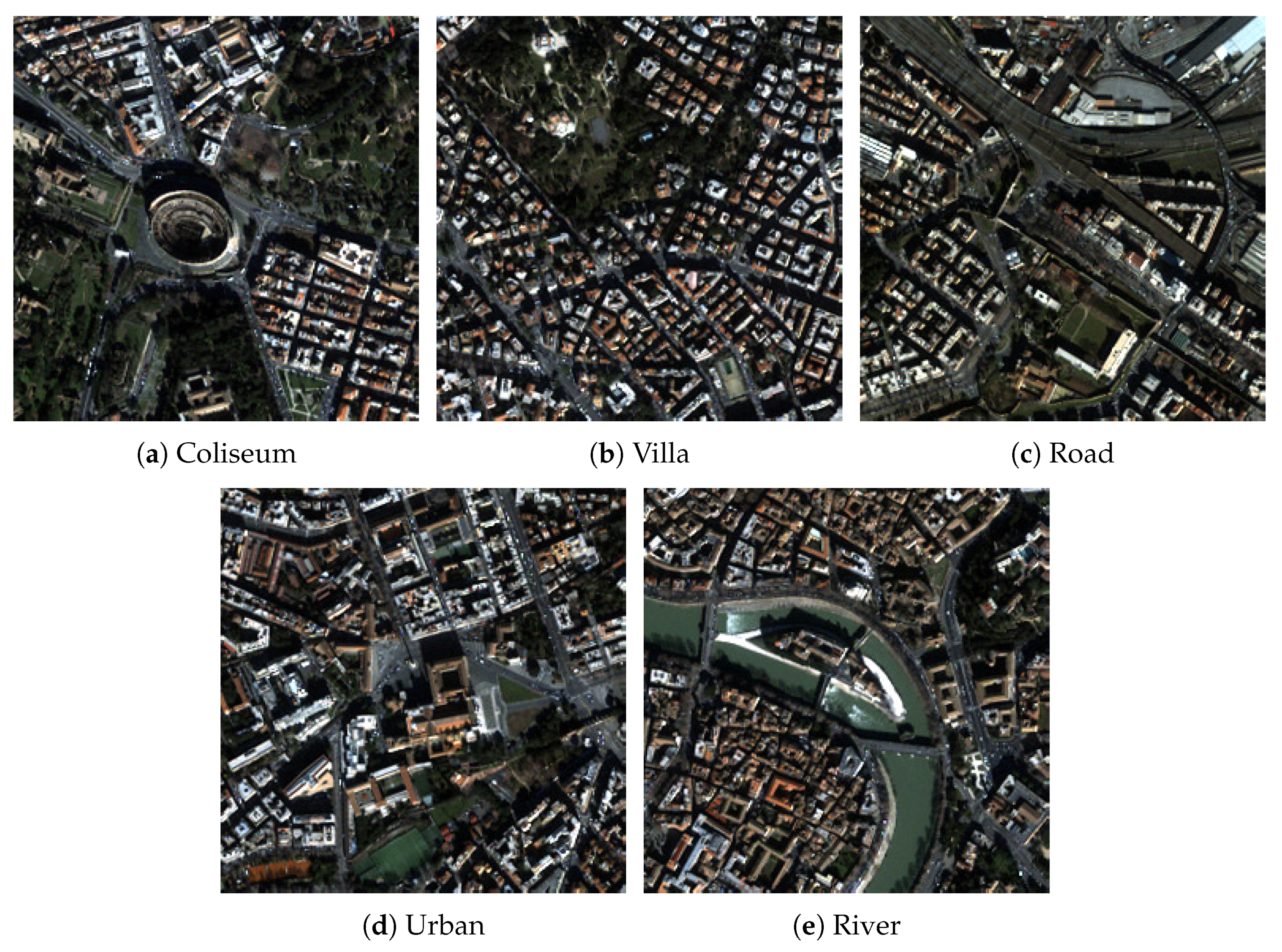
We used the component substitution (CS) and multiresolution analysis (MRA) PS algorithms following [13]. The algorithms were classified into low-, medium-, and high-performance methods based on the scores computed at full- and reduced resolution on the regions of interest (ROI) named Coliseum, Villa, Road, Urban, and River and extracted from dataset IKONOS. Each ROI of 256 × 256 × 4 pixels for MS and 1024 × 1024 pixels for PAN was extracted from specific regions of one larger image of the city of Rome with size of 6452 × 6432 pixels for PAN and 1613 × 1608 × 4 pixels for MS images. The reduced resolution metrics were applied on 64 × 64 × 4 MS images that were obtained by filtering and sub-sampling the original 256 × 256 × 4 MS images. PAN image size was 256 × 256 for this case. We selected one algorithm from each performance group, yielding a set of PS techniques having a wide range of performances. Specifically, we used: [13] (i) CS approaches: principal component analysis (PCA), intensity-hue-saturation (IHS), and band-dependent spatial detail (BDSD); and (ii) MRA methods: a trous wavelet transform using Model 2 (ATWT-M2), high-pass filtering (HPF), and the modulation transfer function Laplacian pyramid with context-based decision (MTF-GLP-CBD).
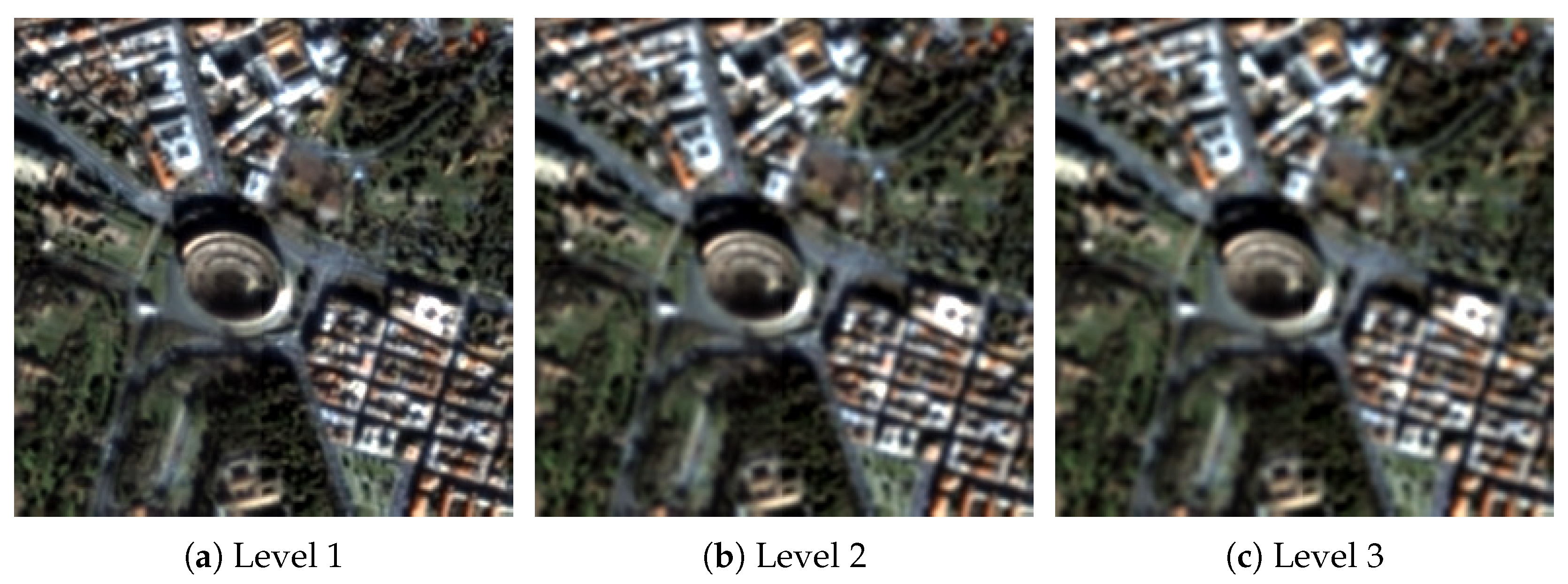
Blur distortion was applied at three levels to the PAN images by defining a Gaussian blur kernel of size 25 × 25 pixels, chosen from . The 33 subjects who participated in the test were students and professors at Pontificia Universidad Javeriana Cali (May 2018), with ages ranging from 18–38 years, without prior experience participating in subjective tests or image quality assessment. The gender ratio of the subjects was 1:3, with less females than males. Before the start of the study, the subjects were explained the different types of distortion present in the images such as artifacts, insufficient color representation, lack of sharpness, and over-/under-exposure as follows:
- Artifacts: noise and blockiness distortions not part of the image content.
- Color: images with incorrect or insufficient color representation.
- Sharpness: general unsharpness, i.e., lack of detail, texture, or sharpness. This distortion differs from out-of-focus distortion in that with sharpness distortion, objects are in focus, but do not appear “crisp” or detailed.
- Exposure: over-/under-exposure, making it difficult to see parts or the entirety of the scene.
At the start of the first session, the subjects had their vision examined using Snellen and Ishihara tests. Test images were displayed to acquaint the participants with the images and the interface. A total of four images with different color representation and distortions were presented to the subjects in the test procedure. These images were not related to the images of the study to avoid biasing the participants. The session routines were developed in MATLAB and the PsychToolbox [39]. The procedure followed the recommendations mentioned in [40], where the subjects indicated the quality of the video on a continuous scale between [0, 100], in which each original image was included in the experiment, but not identified as such. The test was performed with an HP S1933 monitor (18.5”) and an Intel HD 4000 graphic card to observe the images. The screen resolution was set to 1366 × 768 at 60 Hz, at a viewing distance between 45 cm and 55 cm. The stimulus images were displayed at their native resolution to prevent distortions due to scaling operations. Areas outside the images were set to black. In addition, the Spyder5 PRO calibrated the display to an industry color reference standard [41]. The study took place during three sessions of 25 min each with 33 volunteers for a total of 440 images evaluated. The sequence started displaying a single stimulus image for 5 s. Then, the subject rated the image using a continuous sliding quality bar with labels “Bad”, “Poor”, “Fair”, “Good”, or “Excellent” and selected the most relevant distortion doing a keyboard selection.
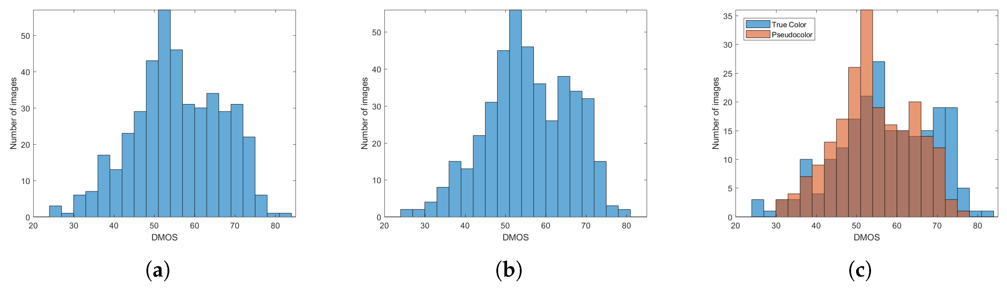
Figure 1 depicts the reference undistorted multi-spectral images scenes: Coliseum, Villa, Road, Urban, and River, used for the subjective study. Examples of the images presented in the subjective study are shown in Figure 2, which depicts a true color image of the Coliseum scene fused with BDSD using a local parameter estimator, distorted with blur and distortion levels. Histograms of the collected differential mean opinion scores (DMOS) are shown in Figure 3, depicting a fairly broad distribution. Scores before subject rejection fell within the range [25, 85], while scores after subject rejection fell within [25, 80], yielding a narrower range of visual quality. DMOS histograms of true color representation has a wider range than pseudo-color representation. This subjective study provided a set of human scores on PS images that supported the design, implementation, and test of NR full-resolution PS image quality metrics in the next section. The results of the subjective study and the proposed image quality analyzers can be found at https://github.com/oscaragudelom/Pansharpening-IQA. In the next section, we present the results of the opinion-aware () and opinion-unaware () quality analyzers.
2.3. Opinion- and Distortion-Unaware Pan-Sharpened Image Quality Analyzer
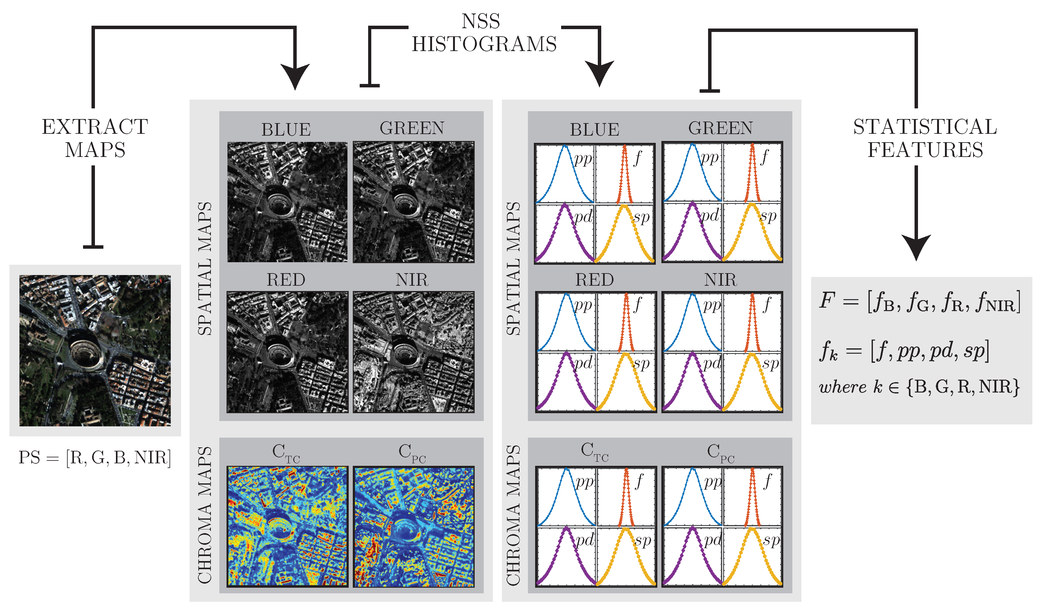
A completely blind image quality analyzer refers to an image quality model that does not require training on databases of human judgments of distorted images and does not rely on training on, or tuning, or any modeling of, or exposure to specific distortions. Instead, a pristine MS image model was constructed from 80 images (each of dimensions 256 × 256) from a region of interest (ROI) of the original MS images from [42]. To ensure independence between the pristine model and the test scores, the ROIs that constituted this model were different from the ROIs selected for use in the subjective study. The idea behind this approach was to measure the dissimilarity between the pristine image model and the test image and use it as a quality measure. A total of 276 features were then extracted, from each image in the pristine set, which were then used to create a pristine model. Since phenomena such as the presence of punctual colored features, saturation, or faded colors affected the visual quality of the PS images, we extracted perceptually-relevant chroma feature maps from true color and false color representations as shown in Figure 4. Chroma feature maps have been employed to learn image features that effectively predict human visual quality judgments of inauthentic and usually isolated (single) distortions in [30]. These feature maps are expressed as a combination of the two chrominance components a* and b* of the CIELAB color space [43] as follows:
Moreover, to capture spatial distortions in the PS images, we deployed features derived from perceptually-relevant bandpass natural scene statistics models of such distorted images based on bandpass statistical image models. In prior research on the quality evaluation of LWIR, fused LWIR and visible, and X-ray images, these models played a key role in the design of successful QA metrics [33,34,44]. Our overall blind IQA models used the following quality-aware processes [34]:
- Mean-subtracted contrast normalized (MSCN) coefficients [45].
- Four “paired products” of horizontal (H), vertical (V), and diagonally-adjacent (D1 and D2) coefficient pairs (which may be viewed as empirical directional correlations) calculated as the products of adjoining MSCN coefficients [23].
- The MSCN coefficients were supplemented by a set of log derivative coefficients (PD1...PD 7), which were intended to provide higher sensitivity to high-frequency noise [46].
- The coefficients obtained from a steerable pyramid image decomposition were used to capture oriented band-pass characteristics, as in [24].
In Figure 4, the feature identifiers that we labeled the MSCN, paired products, paired log-derivatives, and steerable pyramid coefficients with are f, pp, pd, and sp, respectively. Vector is composed of statistical features such as (i) shape and variance extracted from a generalized Gaussian distribution (GGD) that models pp coefficients and (ii) the shape, mean, left variance, and right variance obtained from an asymmetric Gaussian distribution (AGGD) that models the f, pd, and sp coefficients [33]. We built a multivariate Gaussian model (MVG) based on the features extracted from a given image. Thus, the number of features represents the dimensionality of the MVG model. The two parameters of the MVG model (i.e., and ) were estimated as in [32], using a maximum likelihood estimator:
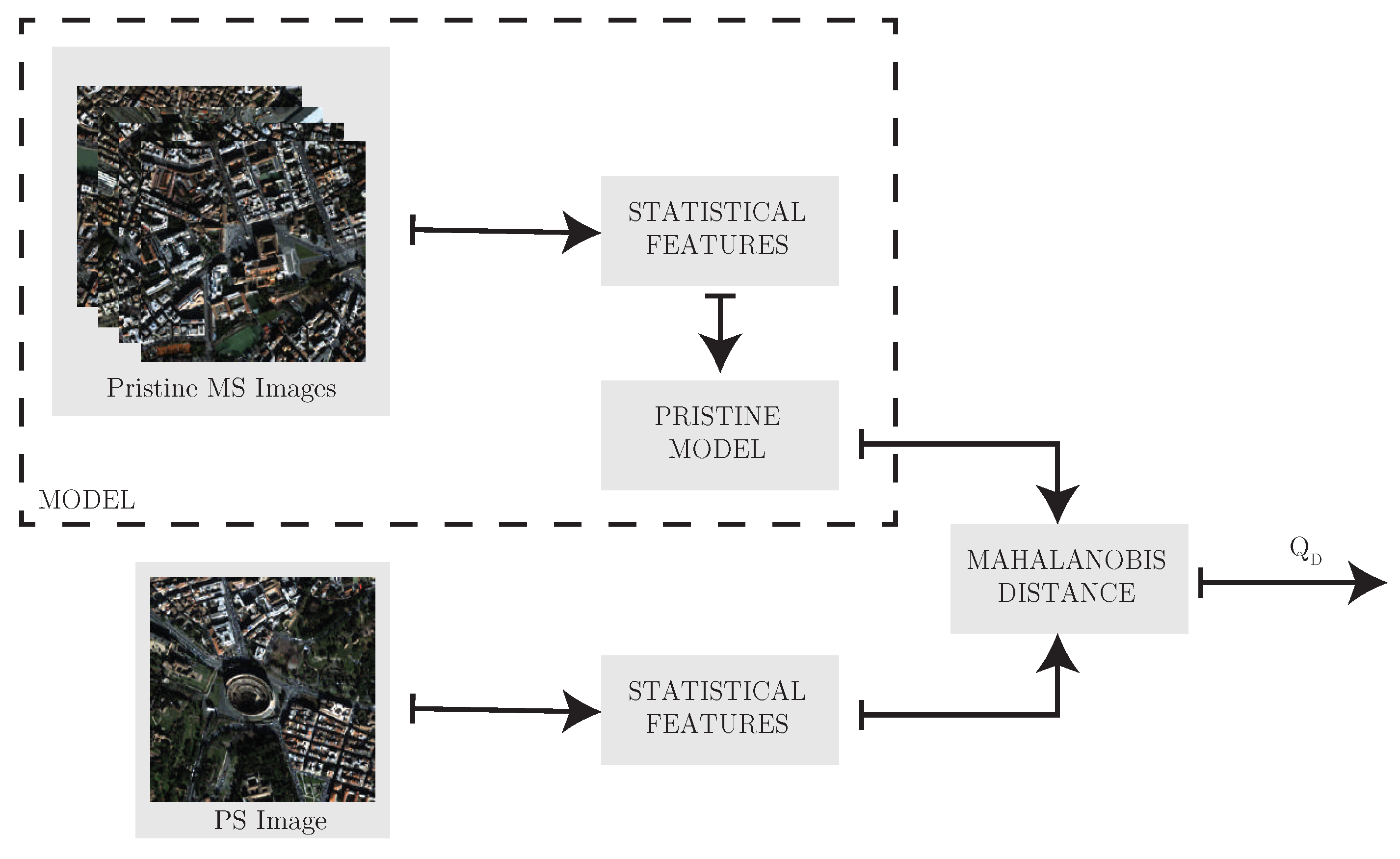
where is the m-dimensional vector that represents the perceptual quality features, denotes the mean vector, and is the co-variance matrix of the MVG model. A set of pristine images (original MS images) and a set of distorted PS images (distorted, down-sampled, then fused) were fitted to the MVG model, making it possible to predict the quality by comparing the pristine model to the model of the degraded image using the Mahalanobis distance:
where , and , are the mean vectors and co-variance matrices of the models obtained with a standard maximum likelihood estimation procedure [47]. and are the quality measures defined on the features extracted only from the spatial map and from the chroma map, respectively. In application and as shown in Figure 5, receives as unique input a fused image and extracts a feature vector with m = 46 × 6 = 276 (46 features extracted from four spatial maps (R, G, B, and NIR) and from two chroma maps, i.e., true color and pseudo-color ). Hence, in Equation (3) = , and , , and are the parameters extracted by the standard maximum likelihood estimation procedure. The pristine model was composed of 80 original MS images deemed to be of high visual quality. No pan-sharpened images were included.
2.4. Opinion-Aware Pan-Sharpened Image Quality Analyzer
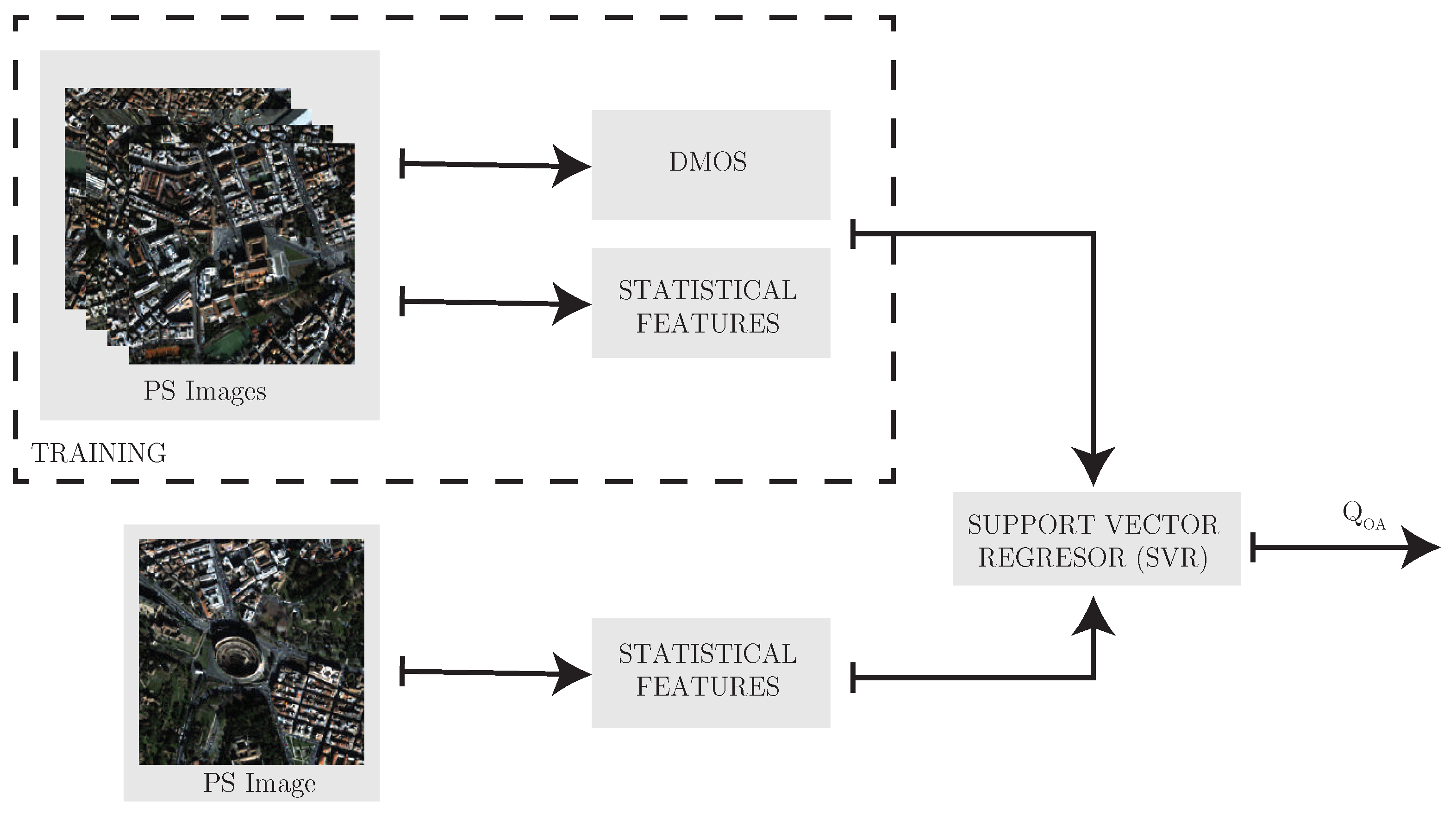
An opinion-aware (OA) quality analyzer refers to a model that has been trained on a database(s) of distorted images with associated human subjective opinion scores. In this case, a mapping is learned from a quality-aware feature space of quality scores using a regression module, yielding an opinion-aware quality model . In our implementation, we used a support vector machine (SVM) regressor (SVR), as shown in Figure 6. This method has been previously applied to IQA using NSS-based features [23,33,34]. SVR is generally noted for being able to handle high-dimensional data, although the framework is generic enough to allow for the use of any regressor. We utilized the LIBSVM package [48] to implement an -SVR with a radial basis function (RBF) kernel, finding the best fitting parameters and using 5-fold cross-validation.
Figure 3 depicts the extraction of the vector F that represents the input quality-aware feature space to the SVR that implements . Since the requires a training procedure, we divided the data from the subjective study into random subsets, where 80% was used for training and 20% for testing, and we took care not to overlap between training and test content. This was done to ensure that results did not depend on features extracted from content, rather than distorted content.
3. Results
The experimental results were developed on the dataset acquired by the sensor, whose characteristics are detailed in [13]. We calculated the geometric mean of the resulting DMOS () obtained by evaluating the true and pseudo-color versions of the PS images in order to generate one score to be mapped by the SVR. In order to account for a possible nonlinear relationship, the scores of the algorithm were passed through a logistic function to fit the objective models to DMOS. Table 2 tabulates the means and standard deviations of 11 reduced resolution, full-resolution, and proposed PS images’ quality analyzers for blurred and undistorted (UD) PS images, while Table 3 presents the analysis for only UD PS images. These scores were obtained from 125 PS images that included 35 UD and 90 blurred PS outcomes. All metric scores indicated better quality results for the UD case. Furthermore, Table 4, Table 5, Table 6, Table 7 and Table 8 show the RRes metrics scores, while Table 9, Table 10, Table 11, Table 12 and Table 13 tabulate the RRes metrics, the proposed PS images’ quality analyzers’ outputs, and the values. The bold numbers in these tables indicate the best performing PS methods. Both sets of metrics were calculated on 35 UD PS images from five different PS scenes extracted from IKONOS satellite images: Villa, Urban, Road, River, and Coliseum. Many results provided by the proposed PS images’ quality analyzers agreed with the human judgments. Furthermore, the proposed PS images’ quality analyzers’ outputs were in line with those obtained at RRes and FRes. We ranked the PS algorithms into high, medium, and low performance according to the scores provided by RRes, RRes, the proposed PS image quality analyzers, and DMOS in Table 14, Table 15, Table 16 and Table 17. These rankings were obtained from 125 PS images that included 35 UD and 90 blurred PS outcomes. The small number of PS techniques evaluated prevented the application of clustering techniques such as k-means. Therefore, to rank the PS techniques, we used the number of times a PS technique was placed in the top three ranks according to a given set of metrics (i.e., RRes, RRes, PS IQA analyzers, or DMOS) to determine its classification as low, medium, or high performance. According to RRes and RRes evaluations, BDSD and MTF-GLP-CBD achieved high and medium performance, while the proposed PS IQA analyzers and DMOS classified BDSD and PCA with high and medium performance. The CS algorithms yielded a higher fidelity in rendering the spatial details in the final image than the MRA techniques. Nonetheless, this usually incurred a higher spectral distortion. This justified the greater alignment between the CS-based algorithms (e.g., BDSD and PCA) and the DMOS data, as shown in Table 18. In fact, Google Earth employs a modified version of the Brovey transformation to sharpen the MS images. Nonetheless, the increment of the spectral distortion of the component substitution methods led to lower performance when indexes such as and were used, as shown in Table 14, where the best approaches were BDSD followed by MTF-GLP-CBD. These results agree with those presented in Vivone et al. [13] when an IKONOS dataset is explored.
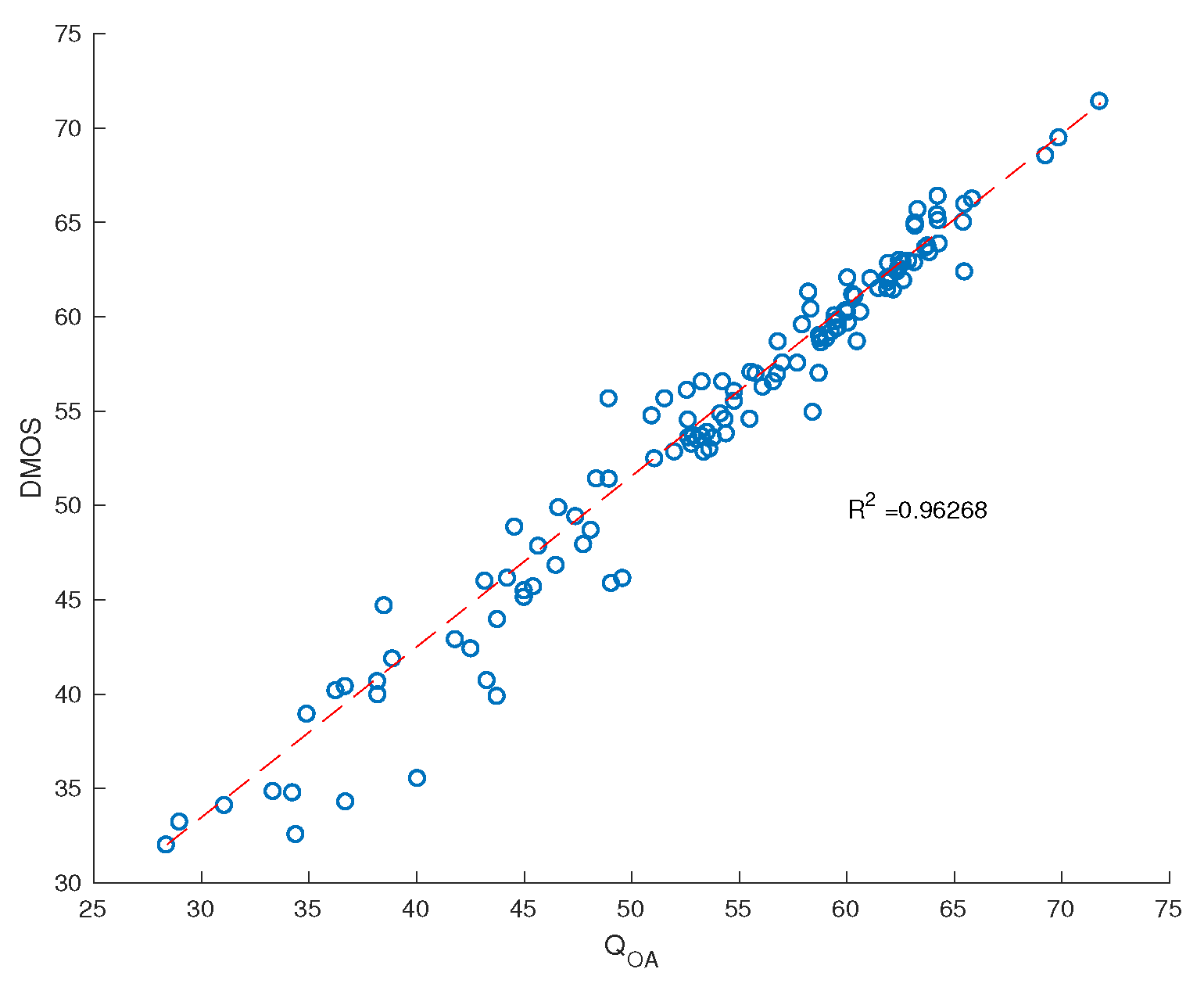
We computed the Spearman rank correlation coefficient (SRCC) and the linear correlation coefficient (LCC), over 1000 iterations for all models, and present their median and standard deviation values in Table 19. The high performance of can be explained by the use of the SVR on a set of data (80% of the acquired samples) that are correlated to the 20% of the samples used for the validation (e.g., samples provided by the same people, scenarios acquired by the same sensor (IKONOS), the same hardware and software exploited for the visual inspection). Furthermore, it is important to notice that the index had access to DMOS scores in the training datasets. Although was the second best model, its performance in terms of the standard deviations of SRCC and LCC was more variable, but it only measured the spatial quality. No information about the spectral quality was included, which limits the assessment of the overall quality of a fusion product. To test whether the results presented in Table 19 are statistically significant, we carried out a non-parametric Kruskal–Wallis statistical significance test on each median value of SRCC between the DMOS and the quality measures (after nonlinear mapping) over 1000 training-test combinations on the dataset. The null hypothesis was that the median SRCC for the algorithm in a row of Table 20 was equal to the median SRCC of the algorithm in a column with a confidence of 95%. The alternate hypothesis was that the median SRCC of the row was greater than or less than the median SRCC of the column. Table 20 tabulates the results of the statistical significance test, where a value of one indicates that the performance of the IQA measure in the row was statistically better than that of the column; zero means that it was statistically worse; and “-” means that it was statistically indistinguishable. From this table, we concluded that the models and produced highly-competitive quality predictions with statistical significance against all of the other quality algorithms tested, while other measures specially designed to evaluate spatial quality such as , , and provided worse correlations against human scores. Since the index is based on RMSE, it is well-known that it has low correlation with human quality perception [49]. This fact limits ’s range of validity. Regarding , it is relevant to point out that the QNR index follows the no reference (NR) paradigm presented in [50], and it is restricted by the validity of assumptions such as the parameters used to combine the two spatial and spectral distortion indexes to get the overall quality index, the use of spatial filters and their design (usually matching the modulation transfer functions of the acquisition devices), and the sensitivity to spatial misalignments. Furthermore, the metrics are different, and the agreement should be found between the and the but always considering that the evaluates the whole image (with a full radiometric range and all bands); instead, we were interested in another issue involving human perception of PS images. Figure 7 depicts the scatter plot of the predicted scores given by our quality model versus DMOS, along with the best fitting logistic function.
4. Discussion
The models and can be seen as supplying additional numerical information with respect to full-resolution protocols (such as and ) that quantitatively assess PS images. This also complements the visual analysis of PS images carried out in previous work that proposed FRes methods, as explained in Section 1. and are also complementary to FRes indices because they measure visual quality with another goal (i.e., prediction of human quality ratings). It is important to notice that and are only one part of the quality assessment procedure and should normally be accompanied by other evaluation protocols, such as those presented in [14,51].
5. Conclusions
NSS are affected by distortions present in PS images, as has been shown in previous work modeling degradation in LWIR, fused LWIR, X-ray, and visible images. NSS proved to be a powerful descriptor, principally when assessing PS images with spatial distortions. Therefore, we proposed both completely blind and opinion-aware fused image quality analyzers whose predictions were highly correlated with human subjective evaluations. This proposed approach intended to support and standardize the visual qualitative evaluation of pan-sharpened images. Our future research plans include more experiments to validate the proposed IQA measures on other classes of satellite data.
Author Contributions
Conceptualization, methodology, and software, O.A.A.-M. and H.D.B.-R.; validation and formal analysis, G.V., A.B., H.D.B.-R., and O.A.A.-M.; writing, review and editing, O.A.A.-M. and H.D.B.-R.
Funding
The authors would like to thank the cooperation of all partners within the Centro de Excelencia y Apropiación en Internet de las Cosas (CEA-IoT) (CEA IoT web page: http://www.cea-iot.org/) project. The authors would also like to thank all the institutions that supported this work: the Colombian Ministry for Information and Communications Technology (Ministerio de Tecnologías de la Información y las Comunicaciones (MinTIC)) and the Colombian Administrative Department of Science, Technology and Innovation (Departamento Administrativo de Ciencia, Tecnología e Innovación-Colciencias) through the Fondo Nacional de Financiamiento para la Ciencia, la Tecnología y la Innovación Francisco José de Caldas (Project ID: FP44842-502-2015). The authors would also like to acknowledge the grant provided by Comision Fulbright Colombia to fund the Visiting Scholar Scholarship granted to H.D.B.-R.
Conflicts of Interest
The authors declare no conflict of interest. The funders had no role in the design of the study; in the collection, analyses, or interpretation of data; in the writing of the manuscript; nor in the decision to publish the results.
References
- Du, Q.; Younan, N.H.; King, R.; Shah, V.P. On the performance evaluation of pan-sharpening techniques. IEEE Geosci. Remote Sens. Lett. 2007, 4, 518–522. [Google Scholar] [CrossRef]
- Souza, C.; Firestone, L.; Silva, L.M.; Roberts, D. Mapping forest degradation in the Eastern Amazon from SPOT 4 through spectral mixture models. Remote Sens. Environ. 2003, 87, 494–506. [Google Scholar] [CrossRef]
- Mohammadzadeh, A.; Tavakoli, A.; Zoej, V.; Mohammad, J. Road extraction based on fuzzy logic and mathematical morphology from pan-sharpened ikonos images. Photogramm. Rec. 2006, 21, 44–60. [Google Scholar] [CrossRef]
- Laporterie-Déjean, F.; de Boissezon, H.; Flouzat, G.; Lefèvre-Fonollosa, M.J. Thematic and statistical evaluations of five panchromatic/multispectral fusion methods on simulated PLEIADES-HR images. Inf. Fusion 2005, 6, 193–212. [Google Scholar] [CrossRef]
- Baronti, S.; Aiazzi, B.; Selva, M.; Garzelli, A.; Alparone, L. A theoretical analysis of the effects of aliasing and misregistration on pansharpened imagery. IEEE J. Sel. Top. Signal Process. 2011, 5, 446–453. [Google Scholar] [CrossRef]
- Palsson, F.; Sveinsson, J.R.; Ulfarsson, M.O. A new pansharpening algorithm based on total variation. IEEE Geosci. Remote Sens. Lett. 2014, 11, 318–322. [Google Scholar] [CrossRef]
- He, X.; Condat, L.; Chanussot, J.M.B.D.J.; Xia, J. A new pansharpening method based on spatial and spectral sparsity priors. IEEE Trans. Image Process. 2014, 23, 4160–4174. [Google Scholar] [CrossRef]
- Vivone, G.; Simões, M.; Dalla Mura, M.; Restaino, R.; Bioucas-Dias, J.M.; Licciardi, G.A.; Chanussot, J. Pansharpening Based on Semiblind Deconvolution. IEEE Trans. Geosci. Remote Sens. 2015, 53, 1997–2010. [Google Scholar] [CrossRef]
- Li, S.; Yang, B. A New Pan-Sharpening Method Using a Compressed Sensing Technique. IEEE Trans. Geosci. Remote Sens. 2011, 49, 738–746. [Google Scholar] [CrossRef]
- Li, S.; Yin, H.; Fang, L. Remote Sensing Image Fusion via Sparse Representations over Learned Dictionaries. IEEE Trans. Geosci. Remote Sens. 2013, 51, 4779–4789. [Google Scholar] [CrossRef]
- Vicinanza, M.R.; Restaino, R.; Vivone, G.; Dalla Mura, M.; Chanussot, J. A Pansharpening Method Based on the Sparse Representation of Injected Details. IEEE Geosci. Remote Sens. Lett. 2015, 12, 180–184. [Google Scholar] [CrossRef]
- Wald, L.; Ranchin, T.; Mangolini, M. Fusion of satellite images of different spatial resolutions: Assessing the quality of resulting images. Photogramm. Eng. Remote Sens. 1997, 63, 691–699. [Google Scholar]
- Vivone, G.; Alparone, L.; Chanussot, J.; Dalla Mura, M.; Garzelli, A.; Licciardi, G.A.; Restaino, R.; Wald, L. A critical comparison among pansharpening algorithms. IEEE Trans. Geosci. Remote Sens. 2015, 53, 2565–2586. [Google Scholar] [CrossRef]
- Khan, M.M.; Alparone, L.; Chanussot, J. Pansharpening Quality Assessment Using the Modulation Transfer Functions of Instruments. IEEE Trans. Geosci. Remote Sens. 2009, 47, 3880–3891. [Google Scholar] [CrossRef]
- Aiazzi, B.; Alparone, L.; Baronti, S.; Carla, R.; Garzelli, A.; Santurri, L. Full scale assessment of pansharpening methods and data products. Proc. SPIE 2014, 9244, 924402-1–924402-22. [Google Scholar]
- Javan, F.D.; Samadzadegan, F.; Reinartz, P. Spatial quality assessment of pan-sharpened high resolution satellite imagery based on an automatically estimated edge based metric. Remote Sens. 2013, 5, 6539–6559. [Google Scholar] [CrossRef]
- Vivone, G.; Restaino, R.; Chanussot, J. A Bayesian Procedure for Full-Resolution Quality Assessment of Pansharpened Products. IEEE Trans. Geosci. Remote Sens. 2018, 56, 4820–4834. [Google Scholar] [CrossRef]
- Kwan, C.; Budavari, B.; Bovik, A.C.; Marchisio, G. Blind quality assessment of fused worldview-3 images by using the combinations of pansharpening and hyper-sharpening paradigms. IEEE Geosci. Remote Sens. Lett. 2017, 14, 1835–1839. [Google Scholar] [CrossRef]
- Alparone, L.; Wald, L.; Chanussot, J.; Thomas, C.; Gamba, P.; Bruce, L.M. Comparison of pansharpening algorithms: Outcome of the 2006 GRS-S data-fusion contest. IEEE Trans. Geosci. Remote Sens. 2007, 45, 3012–3021. [Google Scholar] [CrossRef]
- Toet, A.; Franken, E. Perceptual evaluation of different image fusion schemes. Displays 2003, 24, 25–37. [Google Scholar] [CrossRef]
- Pohl, C.; van Genderen, J.L. Multisensor image fusion in remote sensing: Concepts, methods and applications. Int. J. Remote Sens. 1998, 19, 823–854. [Google Scholar] [CrossRef]
- Chavez, P.; Bowell, J. Comparison of the spectral information content of Landsat Thematic Mapper and SPOT for three different sites in the Phoenix, Arizona Region. ISPRS J. Photogramm. Remote Sens. 1988, 54, 1699–1708. [Google Scholar]
- Mittal, A.; Moorthy, A.K.; Bovik, A.C. No-reference image quality assessment in the spatial domain. IEEE Trans. Image Process. 2012, 21, 4695–4708. [Google Scholar] [CrossRef]
- Moorthy, A.K.; Bovik, A.C. Blind image quality assessment: From natural scene statistics to perceptual quality. IEEE Trans. Image Process. 2011, 20, 3350–3364. [Google Scholar] [CrossRef]
- Olshausen, B.A.; Field, D. Emergence of simple-cell receptive field properties by learning a sparse code for natural images. Nature 1996, 381, 607–609. [Google Scholar] [CrossRef]
- Ruderman, D. The statistics of natural images. Netw. Comput. Neural Syst. 1994, 5, 517–548. [Google Scholar] [CrossRef] [Green Version]
- Simoncelli, E.P.; Olshausen, B.A. Natural image statistics and neural representation. Annu. Rev. Neurosci. 2001, 24, 1193–1216. [Google Scholar] [CrossRef]
- Olshausen, B.A.; Field, D.J. Natural image statistics and efficient coding. Netw. Comput. Neural Syst. 1996, 7, 333–339. [Google Scholar] [CrossRef] [Green Version]
- Saad, M.A.; Bovik, A.C.; Charrier, C. Blind image quality assessment: A natural scene statistics approach in the DCT domain. IEEE Trans. Image Process. 2012, 21, 3339–3352. [Google Scholar] [CrossRef]
- Ghadiyaram, D.; Bovik, A.C. Perceptual quality prediction on authentically distorted images using a bag of features approach. J. Vis. 2017, 17, 32. [Google Scholar] [CrossRef] [Green Version]
- Gupta, P.; Glover, J.; Paulter, N.G., Jr.; Bovik, A.C. Studying the Statistics of Natural X-ray Pictures. J. Test. Eval. 2018, 46, 1478–1488. [Google Scholar] [CrossRef]
- Mittal, A.; Soundararajan, R.; Bovik, A.C. Making a “completely blind” image quality analyzer. IEEE Signal Process. Lett. 2013, 20, 209–212. [Google Scholar] [CrossRef]
- Goodall, T.R.; Bovik, A.C.; Paulter, N.G. Tasking on natural statistics of infrared images. IEEE Trans. Image Process. 2016, 25, 65–79. [Google Scholar] [CrossRef]
- Moreno-Villamarin, D.; Benitez-Restrepo, H.; Bovik, A. Predicting the Quality of Fused Long Wave Infrared and Visible Light Images. IEEE Trans. Image Process. 2017, 26, 3479–3491. [Google Scholar] [CrossRef]
- Yang, J.; Zhao, Y.; Yi, C.; Chan, J.C.W. No-Reference Hyperspectral Image Quality Assessment via Quality-Sensitive Features Learning. Remote Sens. 2017, 9, 305. [Google Scholar] [CrossRef]
- Thomas, C.; Ranchin, T.; Wald, L.; Chanussot, J. Synthesis of multispectral images to high spatial resolution: A critical review of fusion methods based on remote sensing physics. IEEE Trans. Geosci. Remote Sens. 2008, 46, 1301–1312. [Google Scholar] [CrossRef]
- Pohl, C.; Moellmann, J.; Fries, K. Standardizing quality assessment of fused remotely sensed images. Int. Arch. Photogramm. Remote Sens. Spat. Inf. Sci. 2017, 42, 863–869. [Google Scholar] [CrossRef]
- Aiazzi, B.; Alparone, L.; Baronti, S.; Garzelli, A. Context-driven fusion of high spatial and spectral resolution images based on oversampled multiresolution analysis. IEEE Trans. Geosci. Remote Sens. 2002, 40, 2300–2312. [Google Scholar] [CrossRef]
- Brainard, D.H.; Vision, S. The psychophysics toolbox. Spat. Vis. 1997, 10, 433–436. [Google Scholar] [CrossRef]
- Seshadrinathan, K.; Soundararajan, R.; Bovik, A.C.; Cormack, L.K. Study of subjective and objective quality assessment of video. IEEE Trans. Image Process. 2010, 19, 1427–1441. [Google Scholar] [CrossRef]
- Datacolor Spyder5 Family. 2018. Available online: http://www.datacolor.com/photography-design/product-overview/spyder5-family/#spyder5pro (accessed on 11 May 2018).
- Image Copyright DigitalGlobe. 2017. Available online: https://apollomapping.com/ (accessed on 16 April 2018).
- Rajashekar, U.; Wang, Z.; Simoncelli, E.P. Perceptual quality assessment of color images using adaptive signal representation. Proc. SPIE 2010, 7527, 75271L. [Google Scholar]
- Gupta, P.; Sinno, Z.; Glover, J.L., Jr.; Paulter, N.G.; Bovik, A.C. Predicting detection performance on security X-ray images as a function of image quality. IEEE Trans. Image Process. 2019. [Google Scholar] [CrossRef]
- Alparone, L.; Baronti, S.; Garzelli, A.; Nencini, F. A global quality measurement of pan-sharpened multispectral imagery. IEEE Geosci. Remote Sens. Lett. 2004, 1, 313–317. [Google Scholar] [CrossRef]
- Zhang, Y.; Chandler, D.M. No-reference image quality assessment based on log-derivative statistics of natural scenes. J. Electron. Imaging 2013, 22, 043025. [Google Scholar] [CrossRef]
- Bishop, C.M. Pattern Recognition and Machine Learning; Springer: Cambridge, UK, 2006; Volume 60, p. 78. [Google Scholar]
- Chang, C.C.; Lin, C.J. LIBSVM: A library for support vector machines. ACM Trans. Intell. Syst. Technol. (TIST) 2011, 2, 27. [Google Scholar] [CrossRef]
- Wang, Z.; Bovik, A.C. Mean squared error: Love it or leave it? A new look at signal fidelity measures. IEEE Signal Process. Mag. 2009, 26, 98–117. [Google Scholar] [CrossRef]
- Selva, M.; Santurri, L.; Baronti, S. On the Use of the Expanded Image in Quality Assessment of Pansharpened Images. IEEE Geosci. Remote Sens. Lett. 2018, 15, 1–5. [Google Scholar] [CrossRef]
- Alparone, L.; Aiazzi, B.; Baronti, S.; Garzelli, A.; Nencini, F.; Selva, M. Multispectral and panchromatic data fusion assessment without reference. Photogramm. Eng. Remote Sens. 2008, 74, 193–200. [Google Scholar] [CrossRef]
Figure 1.
Reference undistorted multi-spectral images scenes used for the subjective study obtained from [42].
Figure 1.
Reference undistorted multi-spectral images scenes used for the subjective study obtained from [42].

Figure 2.
Example of distortion levels. Three different levels of distortion for (a–c) blur.

Figure 3.
Histograms of the differential mean opinion scores (DMOS) in 33 equally-spaced bins for (a) scores obtained for all images before subject rejection, (b) scores obtained for all images after subject rejection, and (c) scores after subject rejection for true color and pseudo-color image representation in the subjective study.

Figure 4.
The perceptual feature space obtains empirical histograms from space maps (B, G, R, NIR) and chroma true color () and chroma pseudo-color () maps. Chroma maps result from the chrominance components of the TC and PC representations, respectively. Then, the processing models extract statistical features in the vector F. NSS, natural scene statistics.

Figure 5.
Flowchart of the opinion- and distortion-unaware quality analyzer.

Figure 6.
Flow chart of the ODAquality analyzer.

Figure 7.
Scatter plot of prediction scores versus the DMOS for all images assessed in the subjective human study and the best fitting logistic function. Notice the linear relationship with .
Figure 7.
Scatter plot of prediction scores versus the DMOS for all images assessed in the subjective human study and the best fitting logistic function. Notice the linear relationship with .


Table 1.
Description of images employed in the subjective study. TC, true color; PC, pseudo-color; MS, multi-spectral; PS, pan-sharpening.
Table 1.
Description of images employed in the subjective study. TC, true color; PC, pseudo-color; MS, multi-spectral; PS, pan-sharpening.
| TC | PC | |
|---|---|---|
| EXP | 5 | 5 |
| Undistorted MS | 5 | 5 |
| PS images | 125 | 125 |
| Total | 135 | 135 |
Table 2.
Means and standard deviations of quality scores from 11 reduced resolution and full-resolution quality metrics. In this case, each algorithm analyzed 125 PS images affected by three different levels of blur distortion.
Table 2.
Means and standard deviations of quality scores from 11 reduced resolution and full-resolution quality metrics. In this case, each algorithm analyzed 125 PS images affected by three different levels of blur distortion.
| 0.75 | 0.10 | |
| 9.25 | 1.91 | |
| 0.80 | 0.11 | |
| 0.50 | 0.26 | |
| 0.11 | 0.08 | |
| 0.84 | 0.07 | |
| 722.66 | 351.80 | |
| 457.36 | 126.26 | |
| 1508.58 | 443.02 | |
| 5.38 | 1.40 | |
| 54.95 | 8.83 |
Table 3.
Means and standard deviations of quality scores from 11 reduced resolution and full-resolution quality metrics. In this case, each algorithm analyzed 35 PS undistorted images (6 PS algorithms + EXP) in five different scenarios.
Table 3.
Means and standard deviations of quality scores from 11 reduced resolution and full-resolution quality metrics. In this case, each algorithm analyzed 35 PS undistorted images (6 PS algorithms + EXP) in five different scenarios.
| 0.79 | 0.13 | |
| 8.38 | 2.42 | |
| 0.85 | 0.15 | |
| 0.54 | 0.25 | |
| 0.14 | 0.08 | |
| 0.81 | 0.09 | |
| 479.95 | 259.90 | |
| 418.99 | 126.44 | |
| 1182.35 | 379.18 | |
| 4.38 | 1.22 | |
| 47.54 | 11.36 |
Table 4.
IKONOS Roma Villa scene, reduced resolution metrics quantitative results. IHS, intensity-hue-saturation; BDSD, band-dependent spatial detail; ATWT-M2, a trous wavelet transform using Model 2; HPF, high-pass filtering; MTF-GLP-CBD, modulation transfer function Laplacian pyramid with context-based decision. The bold number indicates the best performing PS method according to each quality metric.
| EXP | 0.51 | 13.45 | 0.51 | 0.88 |
| 0.73 | 10.16 | 0.93 | 0.88 | |
| IHS | 0.73 | 10.32 | 0.91 | 0.88 |
| BDSD | 0.93 | 5.61 | 0.95 | 0.87 |
| ATWT-M2 | 0.63 | 11.72 | 0.86 | 0.88 |
| HPF | 0.81 | 8.94 | 0.91 | 0.88 |
| MTF-GLP-CBD | 0.93 | 5.83 | 0.94 | 0.93 |
Table 5.
IKONOS Roma Urban scene, reduced resolution metrics quantitative results. The bold number indicates the best performing PS method according to each quality metric.
Table 5.
IKONOS Roma Urban scene, reduced resolution metrics quantitative results. The bold number indicates the best performing PS method according to each quality metric.
| EXP | 0.60 | 11.89 | 0.50 | 0.48 |
| 0.80 | 8.63 | 0.93 | 0.49 | |
| IHS | 0.80 | 8.58 | 0.93 | 0.49 |
| BDSD | 0.94 | 5.31 | 0.94 | 0.70 |
| ATWT-M2 | 0.70 | 10.27 | 0.86 | 0.48 |
| HPF | 0.86 | 7.58 | 0.91 | 0.51 |
| MTF-GLP-CBD | 0.94 | 5.39 | 0.94 | 0.71 |
Table 6.
IKONOS Roma Road scene, reduced resolution quantitative results. The bold number indicates the best performing PS method according to each quality metric.
Table 6.
IKONOS Roma Road scene, reduced resolution quantitative results. The bold number indicates the best performing PS method according to each quality metric.
| EXP | 0.58 | 11.63 | 0.52 | 0.59 |
| 0.82 | 8.30 | 0.93 | 0.60 | |
| IHS | 0.83 | 8.16 | 0.94 | 0.60 |
| BDSD | 0.94 | 5.18 | 0.95 | 0.70 |
| ATWT-M2 | 0.68 | 10.10 | 0.85 | 0.59 |
| HPF | 0.86 | 7.15 | 0.92 | 0.62 |
| MTF-GLP-CBD | 0.94 | 5.24 | 0.94 | 0.73 |
Table 7.
IKONOS Roma River scene, reduced resolution quantitative results. The bold number indicates the best performing PS method according to each quality metric.
Table 7.
IKONOS Roma River scene, reduced resolution quantitative results. The bold number indicates the best performing PS method according to each quality metric.
| EXP | 0.58 | 10.43 | 0.51 | 0.09 |
| 0.81 | 7.42 | 0.93 | 0.08 | |
| IHS | 0.81 | 7.51 | 0.93 | 0.07 |
| BDSD | 0.95 | 4.45 | 0.95 | 0.61 |
| ATWT-M2 | 0.68 | 9.07 | 0.84 | 0.08 |
| HPF | 0.86 | 6.58 | 0.91 | 0.21 |
| MTF-GLP-CBD | 0.94 | 4.54 | 0.94 | 0.55 |
Table 8.
IKONOS Roma Coliseum scene, reduced resolution quantitative results. The bold number indicates the best performing PS method according to each quality metric.
Table 8.
IKONOS Roma Coliseum scene, reduced resolution quantitative results. The bold number indicates the best performing PS method according to each quality metric.
| EXP | 0.58 | 12.12 | 0.51 | 0.30 |
| 0.73 | 10.34 | 0.87 | 0.31 | |
| IHS | 0.77 | 9.58 | 0.90 | 0.30 |
| BDSD | 0.88 | 6.51 | 0.92 | 0.57 |
| ATWT-M2 | 0.68 | 10.74 | 0.83 | 0.30 |
| HPF | 0.83 | 7.98 | 0.89 | 0.35 |
| MTF-GLP-CBD | 0.88 | 6.61 | 0.91 | 0.51 |
Table 9.
IKONOS Roma Villa scene, full-resolution, image quality assessment metrics, and quantitative results. The bold number indicates the best performing PS method according to each quality metric.
Table 9.
IKONOS Roma Villa scene, full-resolution, image quality assessment metrics, and quantitative results. The bold number indicates the best performing PS method according to each quality metric.
| DMOS-GM | ||||||||
|---|---|---|---|---|---|---|---|---|
| EXP | 0.40 | 0.59 | 1055.62 | 524.89 | 2266.59 | 5.79 | 69.75 | 69.44 |
| 0.13 | 0.84 | 531.40 | 385.05 | 988.53 | 4.85 | 42.96 | 42.86 | |
| IHS | 0.13 | 0.84 | 604.92 | 377.77 | 1208.89 | 4.78 | 51.27 | 46.10 |
| BDSD | 0.05 | 0.88 | 447.97 | 312.53 | 908.14 | 5.77 | 43.88 | 43.92 |
| ATWT-M2 | 0.26 | 0.71 | 1001.56 | 486.65 | 1625.02 | 7.53 | 59.24 | 58.81 |
| HPF | 0.10 | 0.85 | 488.97 | 290.10 | 865.49 | 4.53 | 53.77 | 53.44 |
| MTF-GLP-CBD | 0.06 | 0.85 | 481.73 | 445.63 | 1120.57 | 5.58 | 45.33 | 45.10 |
Table 10.
IKONOS Roma Urban scene, full-resolution, image quality assessment metrics, and quantitative results. The bold number indicates the best performing PS method according to each quality metric.
Table 10.
IKONOS Roma Urban scene, full-resolution, image quality assessment metrics, and quantitative results. The bold number indicates the best performing PS method according to each quality metric.
| DMOS-GM | ||||||||
|---|---|---|---|---|---|---|---|---|
| EXP | 0.26 | 0.74 | 993.92 | 400.93 | 1841.59 | 6.17 | 71.32 | 71.38 |
| 0.07 | 0.90 | 273.39 | 255.64 | 801.77 | 3.56 | 39.31 | 38.90 | |
| IHS | 0.06 | 0.91 | 261.11 | 305.48 | 965.23 | 3.47 | 46.61 | 40.69 |
| BDSD | 0.07 | 0.88 | 265.99 | 311.59 | 843.91 | 4.42 | 42.20 | 39.93 |
| ATWT-M2 | 0.10 | 0.88 | 486.16 | 369.68 | 1148.38 | 6.46 | 61.52 | 60.21 |
| HPF | 0.05 | 0.89 | 271.42 | 203.53 | 828.77 | 3.80 | 50.14 | 49.84 |
| MTF-GLP-CBD | 0.09 | 0.82 | 251.77 | 362.45 | 911.05 | 4.23 | 47.19 | 39.84 |
Table 11.
IKONOS Roma Road scene, full-resolution, image quality assessment metrics, and quantitative results. The bold number indicates the best performing PS method according to each quality metric.
Table 11.
IKONOS Roma Road scene, full-resolution, image quality assessment metrics, and quantitative results. The bold number indicates the best performing PS method according to each quality metric.
| DMOS-GM | ||||||||
|---|---|---|---|---|---|---|---|---|
| EXP | 0.26 | 0.73 | 975.01 | 568.75 | 2023.48 | 5.31 | 65.33 | 64.98 |
| 0.09 | 0.86 | 297.67 | 345.64 | 913.40 | 2.71 | 32.04 | 33.19 | |
| IHS | 0.08 | 0.87 | 272.50 | 444.76 | 1094.48 | 2.62 | 32.11 | 31.97 |
| BDSD | 0.07 | 0.86 | 293.88 | 344.67 | 855.00 | 4.05 | 36.30 | 32.53 |
| ATWT-M2 | 0.11 | 0.87 | 381.90 | 364.40 | 1127.49 | 4.35 | 54.08 | 53.83 |
| HPF | 0.06 | 0.88 | 335.78 | 312.76 | 861.62 | 2.61 | 44.79 | 42.37 |
| MTF-GLP-CBD | 0.09 | 0.83 | 279.91 | 371.91 | 925.52 | 3.70 | 41.69 | 35.50 |
Table 12.
IKONOS Roma River scene, full-resolution, image quality assessment metrics, and quantitative results. The bold number indicates the best performing PS method according to each quality metric.
Table 12.
IKONOS Roma River scene, full-resolution, image quality assessment metrics, and quantitative results. The bold number indicates the best performing PS method according to each quality metric.
| DMOS-GM | ||||||||
|---|---|---|---|---|---|---|---|---|
| EXP | 0.07 | 0.92 | 998.36 | 556.13 | 1872.33 | 4.96 | 68.88 | 68.50 |
| 0.20 | 0.79 | 301.85 | 468.15 | 947.26 | 2.50 | 39.39 | 40.14 | |
| IHS | 0.20 | 0.78 | 307.58 | 579.74 | 1252.39 | 2.49 | 40.98 | 40.63 |
| BDSD | 0.07 | 0.88 | 298.84 | 499.56 | 954.65 | 3.61 | 39.36 | 40.37 |
| ATWT-M2 | 0.08 | 0.91 | 461.56 | 765.40 | 1438.87 | 3.71 | 59.04 | 56.96 |
| HPF | 0.14 | 0.81 | 312.69 | 521.22 | 978.25 | 2.59 | 47.73 | 48.82 |
| MTF-GLP-CBD | 0.11 | 0.81 | 276.91 | 497.61 | 930.82 | 3.42 | 41.15 | 41.83 |
Table 13.
IKONOS Roma Coliseum scene, full-resolution, image quality assessment metrics, and quantitative results. The bold number indicates the best performing PS method according to each quality metric.
Table 13.
IKONOS Roma Coliseum scene, full-resolution, image quality assessment metrics, and quantitative results. The bold number indicates the best performing PS method according to each quality metric.
| DMOS-GM | ||||||||
|---|---|---|---|---|---|---|---|---|
| EXP | 0.10 | 0.86 | 978.35 | 641.87 | 1787.43 | 5.20 | 63.04 | 62.91 |
| 0.27 | 0.63 | 616.29 | 210.12 | 1244.64 | 4.75 | 35.28 | 34.26 | |
| IHS | 0.26 | 0.65 | 396.08 | 621.18 | 1396.54 | 4.08 | 35.22 | 34.74 |
| BDSD | 0.16 | 0.73 | 291.14 | 346.07 | 874.35 | 4.94 | 33.39 | 34.07 |
| ATWT-M2 | 0.09 | 0.84 | 451.73 | 458.47 | 1313.14 | 4.95 | 54.03 | 53.64 |
| HPF | 0.20 | 0.69 | 464.43 | 316.12 | 1143.46 | 4.44 | 40.65 | 44.65 |
| MTF-GLP-CBD | 0.20 | 0.66 | 389.77 | 398.16 | 1123.17 | 5.46 | 34.91 | 34.81 |
Table 14.
Clustering of pan-sharpening algorithms applied to IKONOS Roma Villa, Urban, Road, River, and Coliseum scenes’ data into high, medium, and low performance. Input data for clustering are the reduced resolution scores indexes , , , and in Table 4, Table 5, Table 6, Table 7 and Table 8.
| High | Medium | Low | |
|---|---|---|---|
| Villa | MTF-GLP-CBD | BDSD | HPF |
| Urban | BDSD | MTF-GLP-CBD | HPF |
| Road | BDSD | MTF-GLP-CBD | HPF |
| River | BDSD | MTF-GLP-CBD | HPF |
| Coliseum | BDSD | MTF-GLP-CBD | HPF |
Table 15.
Clustering of pan-sharpening algorithms applied to IKONOS Roma Villa, Urban, Road, River, and Coliseum scenes’ data into high, medium, and low performance. Input data for clustering are the full-resolution index in Table 9, Table 10, Table 11, Table 12 and Table 13.
| High | Medium | Low | |
|---|---|---|---|
| Villa | BDSD | MTF-GLP-CBD | HPF |
| Urban | IHS | PCA | HPF |
| Road | HPF | IHS | ATWT-M2 |
| River | ATWT-M2 | BDSD | MTF-GLP-CBD |
| Coliseum | ATWT-M2 | BDSD | HPF |
Table 16.
Clustering of pan-sharpening algorithms applied to IKONOS Roma Villa, Urban, Road, River, and Coliseum scenes’ data into high, medium, and low performance. Input data for clustering are the full-resolution image quality assessment (IQA)-based indexes , , , and , in Table 9, Table 10, Table 11, Table 12 and Table 13.
| High | Medium | Low | |
|---|---|---|---|
| Villa | BDSD | HPF | PCA |
| Urban | PCA | IHS | BDSD |
| Road | PCA | BDSD | IHS |
| River | PCA | BDSD | MTF-GLP-CBD |
| Coliseum | BDSD | IHS | HPF |
Table 17.
Clustering of pan-sharpening algorithms applied to IKONOS Roma Villa, Urban, Road, River, and Coliseum scenes’ data into high, medium, and low performance. Input data for clustering are the IQA-based indexes , , , , and in Table 9, Table 10, Table 11, Table 12 and Table 13.
| High | Medium | Low | |
|---|---|---|---|
| Villa | PCA | BDSD | MTF-GLP-CBD |
| Urban | PCA | BDSD | MTF-GLP-CBD |
| Road | PCA | IHS | BDSD |
| River | PCA | IHS | BDSD |
| Coliseum | PCA | IHS | BDSD |
Table 18.
Means () and standard deviations () of for each PS technique extracted from 30 PS undistorted images (6 PS algorithms) in five different scenarios). The PS techniques are organized from high to low performance.
Table 18.
Means () and standard deviations () of for each PS technique extracted from 30 PS undistorted images (6 PS algorithms) in five different scenarios). The PS techniques are organized from high to low performance.
| BDSD | 37.87 | 4.07 |
| PCA | 38.16 | 4.74 |
| IHS | 38.82 | 5.55 |
| MTF-GLP-CBD | 39.41 | 4.33 |
| ATWT-M2 | 47.82 | 4.37 |
| HPF | 56.69 | 2.93 |
Table 19.
Median and standard deviation of the Spearman rank correlation coefficient (SRCC) and the linear correlation coefficient (LCC) between DMOS and spatial quality indices measured over 1000 iterations.
Table 19.
Median and standard deviation of the Spearman rank correlation coefficient (SRCC) and the linear correlation coefficient (LCC) between DMOS and spatial quality indices measured over 1000 iterations.
| 0.6692 | 0.1040 | 0.6739 | 0.1029 | 7.1022 | 1.1542 | |
| 0.6146 | 0.1171 | 0.6352 | 0.1191 | 7.4441 | 1.2732 | |
| 0.8408 | 0.0633 | 0.8668 | 0.0487 | 4.7596 | 0.8503 | |
| 0.1502 | 0.1126 | 0.1249 | 0.1034 | 9.3622 | 1.1801 | |
| 0.1482 | 0.1201 | 0.1379 | 0.1145 | 9.2684 | 1.3716 | |
| 0.1564 | 0.1281 | 0.1515 | 0.1214 | 9.1547 | 1.3583 | |
| 0.8096 | 0.0753 | 0.8229 | 0.0810 | 5.6903 | 1.3099 | |
| 0.2153 | 0.1446 | 0.2264 | 0.1428 | 9.0588 | 1.2170 | |
| 0.7762 | 0.0727 | 0.7671 | 0.0931 | 6.3339 | 1.2881 | |
| 0.5496 | 0.1350 | 0.5931 | 0.1257 | 7.6390 | 1.1749 | |
| 0.9262 | 0.0416 | 0.9374 | 0.0289 | 4.8784 | 1.0508 |
Table 20.
Statistical significance matrix of SRCC between DMOS and quality indices.
| - | 1 | 0 | 1 | 1 | 1 | 0 | 1 | 0 | 1 | 0 | |
| 0 | - | 0 | 1 | 1 | 1 | 0 | 1 | 0 | 1 | 0 | |
| 1 | 1 | - | 1 | 1 | 1 | 1 | 1 | 1 | 1 | 0 | |
| 0 | 0 | 0 | - | - | - | 0 | 0 | 0 | 0 | 0 | |
| 0 | 0 | 0 | - | - | - | 0 | 0 | 0 | 0 | 0 | |
| 0 | 0 | 0 | - | - | - | 0 | 0 | 0 | 0 | 0 | |
| 1 | 1 | 0 | 1 | 1 | 1 | - | 1 | 1 | 1 | 0 | |
| 0 | 0 | 0 | 1 | 1 | 1 | 0 | - | 0 | 0 | 0 | |
| 1 | 1 | 0 | 1 | 1 | 1 | 0 | 1 | - | 1 | 0 | |
| 0 | 0 | 0 | 1 | 1 | 1 | 0 | 1 | 0 | - | 0 | |
| 1 | 1 | 1 | 1 | 1 | 1 | 1 | 1 | 1 | 1 | - |
© 2019 by the authors. Licensee MDPI, Basel, Switzerland. This article is an open access article distributed under the terms and conditions of the Creative Commons Attribution (CC BY) license (http://creativecommons.org/licenses/by/4.0/).
Share and Cite
MDPI and ACS Style
Agudelo-Medina, O.A.; Benitez-Restrepo, H.D.; Vivone, G.; Bovik, A. Perceptual Quality Assessment of Pan-Sharpened Images. Remote Sens. 2019, 11, 877. https://0-doi-org.brum.beds.ac.uk/10.3390/rs11070877
AMA Style
Agudelo-Medina OA, Benitez-Restrepo HD, Vivone G, Bovik A. Perceptual Quality Assessment of Pan-Sharpened Images. Remote Sensing. 2019; 11(7):877. https://0-doi-org.brum.beds.ac.uk/10.3390/rs11070877
Chicago/Turabian StyleAgudelo-Medina, Oscar A., Hernan Dario Benitez-Restrepo, Gemine Vivone, and Alan Bovik. 2019. "Perceptual Quality Assessment of Pan-Sharpened Images" Remote Sensing 11, no. 7: 877. https://0-doi-org.brum.beds.ac.uk/10.3390/rs11070877
Note that from the first issue of 2016, this journal uses article numbers instead of page numbers. See further details here.