Towards Uniform Point Density: Evaluation of an Adaptive Terrestrial Laser Scanner


1
Lyles School of Civil Engineering, Purdue University, West Lafayette, IN 47907, USA
2
Geospatial Research Lab, Corbin Field Station, 15319 Magnetic Lane, Woodford, VA 22580, USA
3
Blackmore Sensors and Analytics, Inc., Bozeman, MT 59718, USA
*
Author to whom correspondence should be addressed.
Remote Sens. 2019, 11(7), 880; https://0-doi-org.brum.beds.ac.uk/10.3390/rs11070880
Submission received: 28 February 2019
/
Revised: 5 April 2019
/
Accepted: 5 April 2019
/
Published: 11 April 2019
Abstract
:One of the intrinsic properties of conventional terrestrial laser scanning technology is the unevenness of its point density over the scene where objects rendered closer to the scanner are more densely covered than the ones far away. This uneven distribution can be amplified as the working range of a laser scanner gets longer. In such case a higher pulse repetition rate (PRR) is applied to the whole scanning area and the scanning time will be dramatically increased. To improve the efficiency of the conventional laser scanning technology, a prototype of adaptive scanning technology, the HRS3D-AS scanner has been developed by Blackmore Sensors and Analytics, Inc. This paper briefly describes the working principles of the adaptive scanner and presents a thorough evaluation on the distributions of the point density in comparison to the conventional scanning. Based on this study, we show that such a new technology can produce a point cloud of more uniform density and less data volume. The overall field scanning time can be reduced by several times compared to the conventional, PRR-fixed scanning. Such properties are expected to significantly simplify the algorithmic development and increase the productivity in data acquisition and processing. The limitations of this new adaptive scanning technology are also discussed in terms of redundant and unresolved details. Finally, recommendations related to the practicing of such adaptive scan are discussed.
1. Introduction
Point density, commonly described by the number of lidar (light detection and ranging) measured points per unit area on a given target [1], is one of the most important metrics that characterizes the quality of point clouds produced by topographic laser scanners [1,2,3]. Nonuniformity of point density is a common problem in terrestrial laser scanning (TLS) since the targets far away from the scanner are more sparely measured than closer objects. Simply increasing the pulse repetition rate will improve the point density in the far field with sacrifice the efficiency of the system. First, it will make the close field-point density much denser. Furthermore, the scanning time over the study area will dramatically increase. Factors influencing the spatial point density of TLS include: the scan pattern, scan rate and pulse repetition rate (PRR). Proper design and operation to achieve an ideal spatial point density throughout an acquired scene has become an important and difficult topic.
Due to the unavoidable existence of nonuniformity in point density, many studies have been undertaken reporting on the effect of point density relating to lidar data processing and information extraction. Such studies include theoretical studies on single-beam laser [4] and multi-beam laser [5], where the point distribution on a simulated hollow sphere surrounding the sensor is simulated and analyzed. Empirical works include the effect of point density on canopy height [6], biomass estimation [7,8,9], tree structure delineation [10], and the measurement accuracy of forestry in general [11]. The quality of building extraction affected by point density was also discussed by [12,13]. Given the nonuniformity of point density, people intended to find more optimal and reasonable ways to define and calculate the point density [14,15] or to preprocess point clouds to generate uniform point density [16]. Even more challenging is that uneven point density can considerably affect the performance of point cloud processing algorithms. For example, a fundamental point cloud processing algorithm is normal estimation, which is closely related to point density. Nonuniform point density makes it difficult to define a stable neighborhood of a point to estimate normal vector, consequently causing errors in point cloud registration [17,18], point cloud feature calculation [19], calibration of spinning actuated lidar scanner [20]. Recent efforts have been made in developing a variety of robust approaches for information extraction from lidar point clouds [21,22,23].
Besides the quality of the data and performance of the data processing, another problem conventional TLS has is efficiency or productivity, i.e., collecting minimal amount of data within least amount of time to reliably meet the need of an application. When scanning, nearly all terrestrial commercial laser scanners apply a “full dome” scanning approach. This means the instrument scans the scene at a fixed angular resolution (i.e., angular sampling density) and PRR regardless of the target’s range. Some suggested to rotate the scanner with high frequency to acquire dense point clouds [24]. This usually results in an over-sampled, large number of pulses being generated to the detriment of the scene. Moreover, scanning at a high frequency would detract the accuracy of point cloud [24]. Reference [25] has pointed out that there should be a trade-off between sampling density and scanning duration as well as the amount of data produced.
This paper introduces a new paradigm of terrestrial laser scanning and evaluates its performance. The prototype scanner, HRS3D-AS is an adaptive scanner which intends to collect point clouds with uniform density regardless of the distance to the scanner. Our testing and evaluation focused on the spatial distribution of point density with the objective to understand the properties of this new scanning technology in terms of its expected design specifications and resulting data quality.
2. Principles of the Adaptive Scanning
The prototype terrestrial scanner HRS3D-AS (adaptive scanner) to be evaluated is developed by Blackmore Sensors and Analytics, Inc. (https://blackmoreinc.com/). It is a significant upgrade from its precursor HRS-3D, which was first reported by its designer and developer in [26,27]. This equipment is based on the principle of frequency modulated continuous waveform (FMCW) laser ranging or laser detection and ranging (LADAR). In comparison to conventional laser scanners, a FMCW system has several key advantages as it outperforms the conventional pulsed system in terms of range resolution, obscurant penetration, and maximum working range [26,27]. As a function of frequency-based technology, a FMCW scanner can provide Doppler imaging and detect moving objects. Such scanner also requires lower power to realize greater range measurement than conventional systems [26]. The “probing” signal used in FMCW system helps it overcome the inability to scale power in linear mode systems, thus improving the system in both range and signal fidelity [27]. It should be noted HRS3D-AS does not use pulsed laser and its optical output is continuous wave. The term MRR or measurement repetition rate should be used to describe the measurement speed of the scanner. Nonetheless, the lidar industry has standardized on the term “pulse repetition rate”, or “PRR”. To avoid confusion, we often use the term PRR colloquially despite its inaccurate description of the sensors’ internal working principles.
This paper evaluates a unique characteristic of the scanner newly available in HRS3D-AS, i.e., the ability of adjusting angular resolution and PRR to achieve a uniform spatial resolution in the resultant point cloud. The basic specifications of HRS3D-AS are summarized in Table 1.
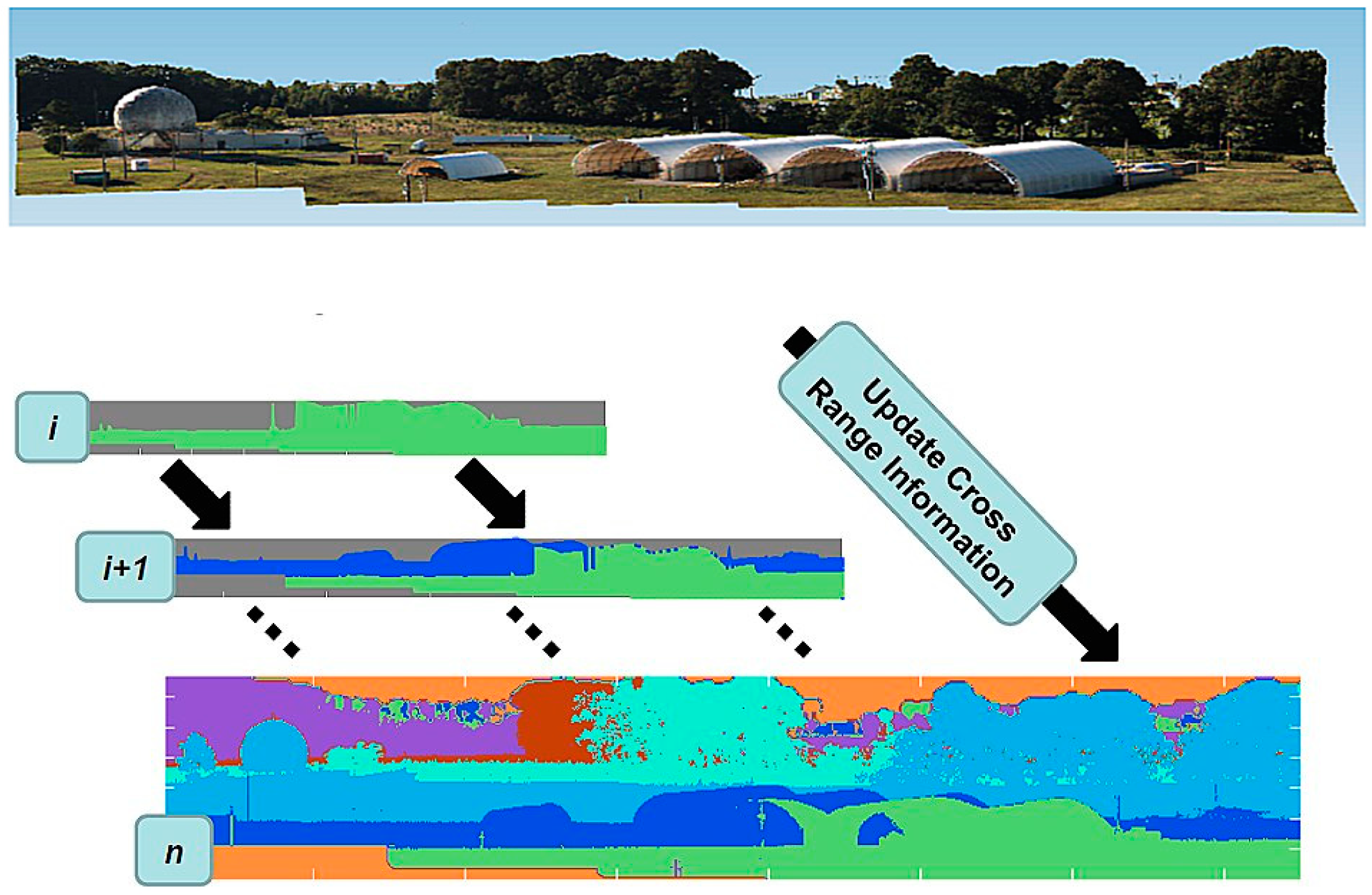
To help accomplish this, the adaptive scanner can work under two modes, conventional single frequency and adaptive multi-frequency. The conventional mode separately scans the scene with a constant angular resolution and PRR, while the adaptive mode works with varying angular resolutions and PRR that maintain high point densities for targets at greater distances in a scene. When operating in the adaptive mode, the scanner first performs an initial coarse, overview scan (under one user-selected pulse repetition rate or PRR) of a scene with a relatively low PRR. This overview scan allows the instrument to divide the scene into several irregular zones according to the distances measured to the targets. As shown in Figure 1, the subsequent scan will then be carried out zone-by-zone, from near (zone 1) to distant (zone n), at the corresponding PRRs and angular resolutions. In summary, the constant angular resolution and PRR of a conventional laser scanner often result in sparser point spacing in distant areas while close range areas are over-sampled. The adaptive mode adjusts the angular resolution and PRR based on the measured zoning distances to the targets so that the point spacing or density can be as even as possible over the entire scene. Table 2 lists the equipment-programmed zone designations and their corresponding ranges and frequencies for the HRS3D-AS scanner.
However, it should be noted that the point density is not mathematically truly uniform. The adaptive scanning algorithm is designed to ensure a minimum sample density is achieved everywhere in the scene. For example, users can request that samples be no more than 5 cm apart. This maximum on-target sample spacing will be respected, but samples will be denser than this spacing at some locations within the scene. Moreover, not all of the zones are used in a scan since the scene may not contain targets at the farther ranges.
3. Study Area and Data
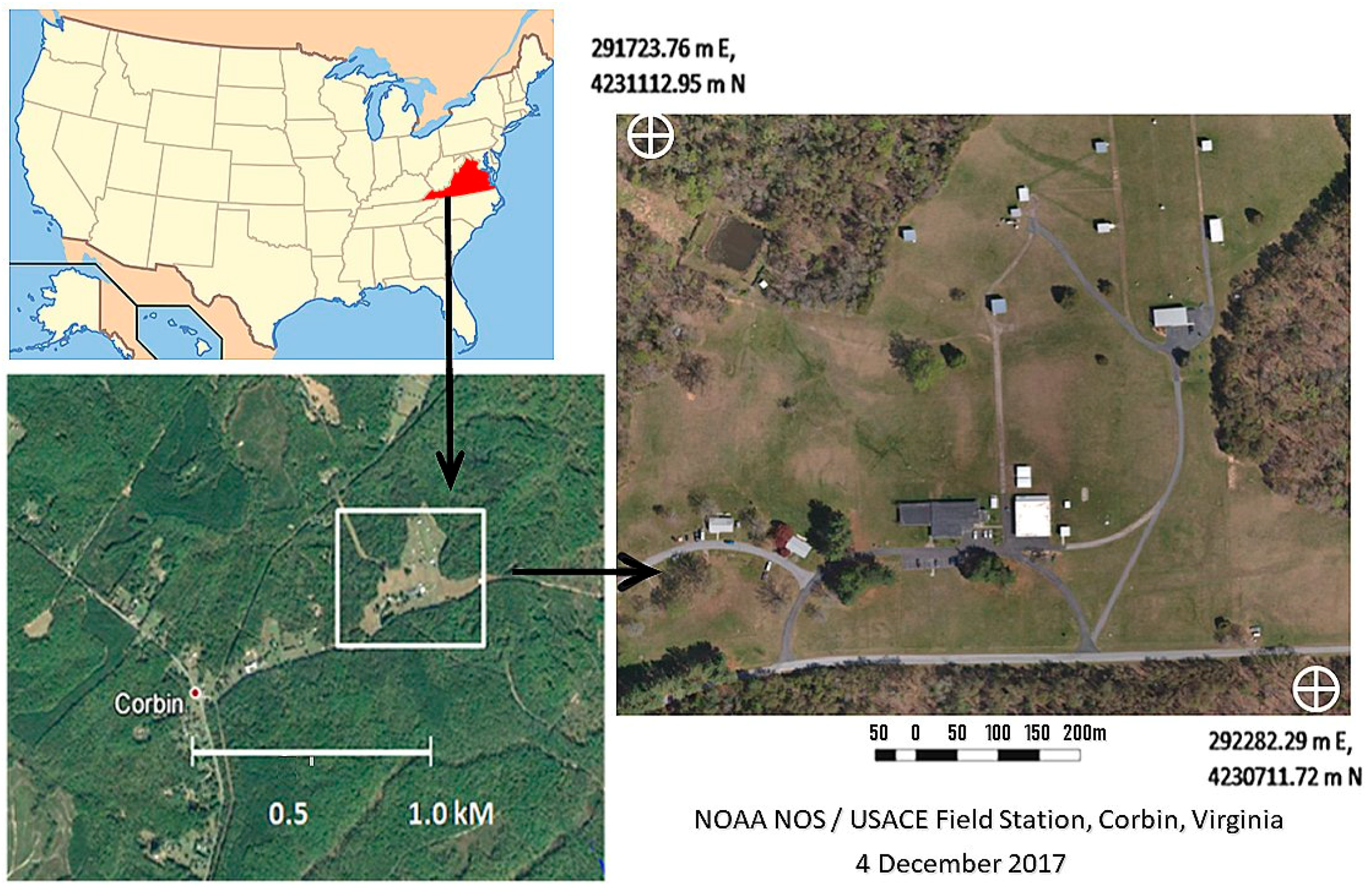
The area selected for this study was the National Oceanic and Atmospheric Administrations, National Ocean Service (NOAA NOS) geodetic surveying training facility at Corbin, Virginia (Figure 2). The area (UTM, Zone 18N scene center 292060.83 m E, 4250963.83 m N) is a 120-hectare, semi-wooded and open site characterized by both deciduous and coniferous trees and rolling topography. The facility is a dedicated center for high accuracy geodetic mapping, unmanned aerial vehicle research and testing, and laser scanner evaluation. Geometric control targets used for this study were previously established during the summer of 2017 and surveyed using high precision GPS (global positioning system) by rapid-static method resulting in sub-centimeter accuracies. All control data were processed using NOAA’s NGS OPUS (On-Line Positioning User Service) and the NovAtel Grafnet (Alberta, Canada) surveying package and placed in the WGS 84 horizontal datum in UTM Zone 18N coordinates using the NAVD 88 vertical datum.
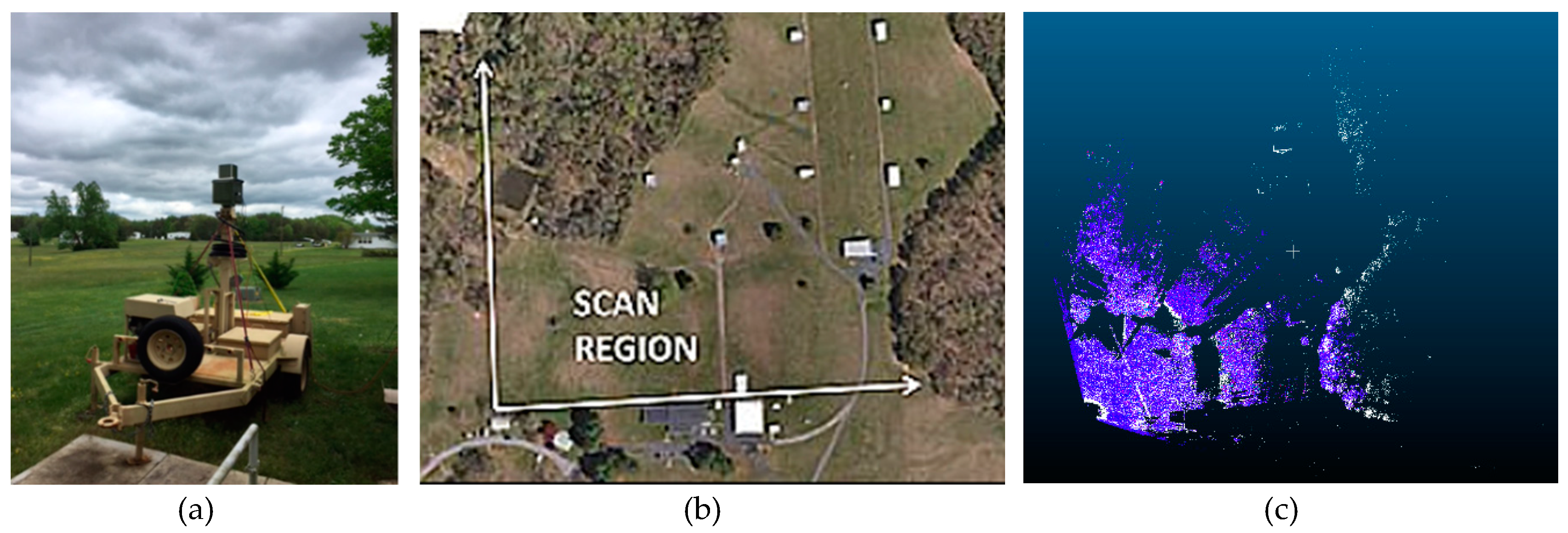
Scene acquisition was accomplished by placing the HRS3D-AS on a deployable tower and elevating the unit 3.05 m above the ground as shown in Figure 3a. To compare data integrity, the same scene was scanned separately using both conventional and adaptive modalities with the HDS3D-AS scanner. Figure 3b depicts the scan region. Figure 3c shows that the point clouds of these two modes mostly overlap, while the maximum range of the conventional mode is larger than the adaptive one.
During the experiment, the scanning range for both the conventional and adaptive collections were set as 1500 m and the resolution was set as 10 mm. During the adaptive scanning, both the horizontal and vertical scanning speed were automatically adjusted according to those scanning parameters and the zone designation shown in Table 2. During the conventional scanning, the PRR was fixed as 48 kHz. The summary of the data collections is shown in Table 3. Initially, the Z range of the adaptive point cloud is from 23.7 m to 56 m; the Z range of the conventional point cloud is from 11.2 m to 107.2 m. However, there are only less than 1% points in the low range (11.20–50.00 m) and high range (90.00–107.20 m). After filtering, the Z range of conventional dataset becomes 60.2 m to 81.1 m. Similarly, we filtered the adaptive dataset and the Z range of the adaptive dataset became 59.8 m to 85.4 m. It should be noted the comparative analysis only makes sense when the two scanning modes yield approximately the same of amount of data. The conventional mode produced about 26.9% more points in total than the adaptive mode does, whereas this number is respectively 152.4% for ground points and 8.6% for non-ground.
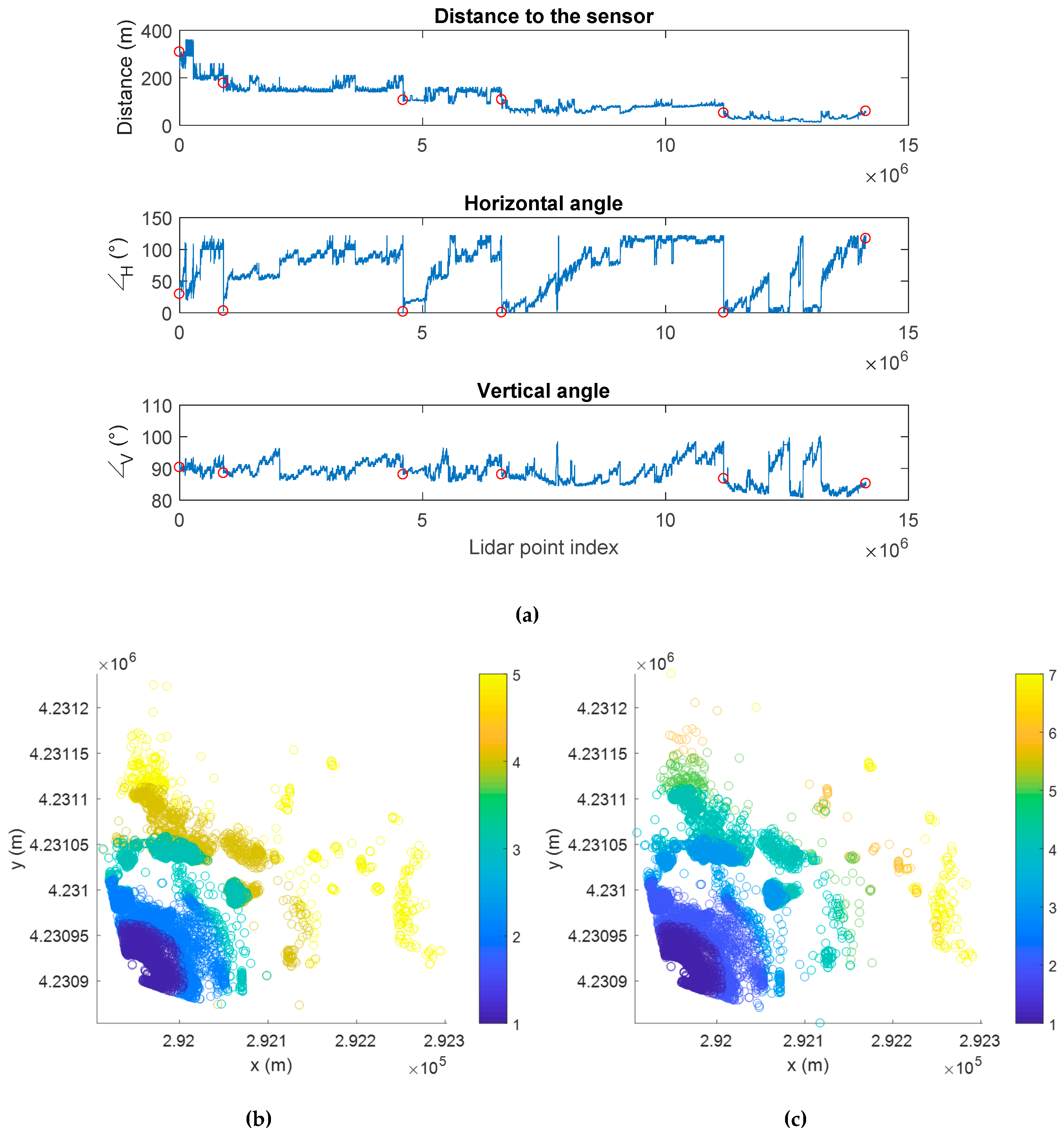
The zone information, i.e., the zone ID for a point in the point clouds may be useful for evaluation. In this study, the adaptive mode started with an overview scan at a frequency of 48 kHz. The results were then stored as a spate overview file. During the subsequent zone-targeted scan, the instrument stored the data according to their zone ID, i.e., each zone has its own file. In this study, a total of seven zone files has 14,122,242 points, whereas there are only 1,605,184 points in the overview scan, i.e., about 11.37% of the zone files. As an option, all the zone files may be combined into one file and provided to the end user. Under such scenario, we need to derive the zone information from the combined adaptive point cloud. For this purpose, we plotted the distances-to-sensor, vertical angle and horizontal angle of all points in the order of their collection. The results are shown in Figure 4a. The lidar points where their horizontal angles are 90 degrees were taken as at the zone boundary. The derived zones were then shown in Figure 4b. For comparison purpose, all the seven zone files were plotted one by one in Figure 4c. It should be noted that this zone re-engineering process may not be able to discover all of the zone information. Some of the zones distant to the scanner may not be separated.
All lidar points were classified to ground points and non-ground points so that their densities could be examined separately. The tool we used was LASTools (https://rapidlasso.com/lastools/).
4. Distribution of Point Density
The central idea of the adaptive scanning is to generate a point cloud with evenly distributed points. To achieve this, we will explore the point density from three aspects: (1) 1-D distribution in terms of distance to the sensor; (2) 2-D distribution of the lidar points; and (3) 2-D Fourier analysis or spectral distribution of the point density.
4.1. 1-D Spatial Analysis
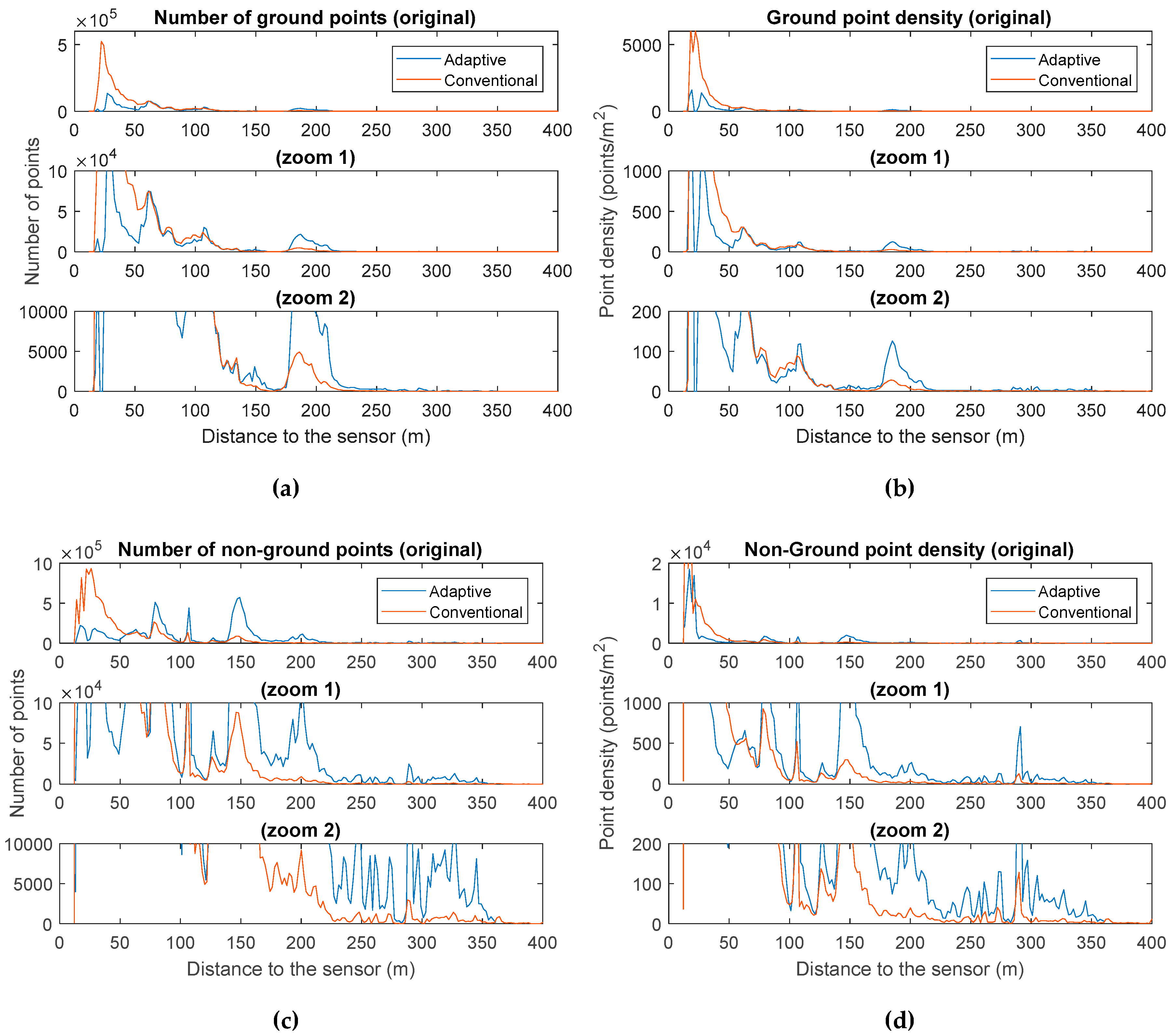
First, we compare the adaptive and the conventional modes by plotting the number of points and the point density in terms of their distances to the scanner. After dividing the entire area into 1 m × 1 m cells, we counted the number of points for each cell. The distances from cells to the scanner were then binned at an interval of two meters. We counted the number of points within each distance bin; and the corresponding point density was calculated by dividing the number of points with the number of non-empty cells. This process was repeated for the ground lidar points and non-ground lidar points, respectively. Figure 5 plots the number of points and point density in terms of the binned distances to the scanner. For purpose of comparison, two zoomed-in plots were also provided to show the fine details. These plots were created for ground points and non-ground points separately. In this study, we found the transition distance is around 150 m for ground points: the conventional mode generates more points when the distance is less than 150 m, whereas the adaptive mode generates more points beyond this distance. For the non-ground points, the transition distance is at 60–70 m. Apparently, these are products of the user-selected parameters. In general, in conventional mode, the user selects a PRR with which to sample the entire scene. In adaptive mode, the user selects a maximum acceptable on-target sample spacing. The transition range between which mode produces the most dense samples is directly depending upon the user-selected parameters in each scan.
4.2. 2-D Spatial Analysis
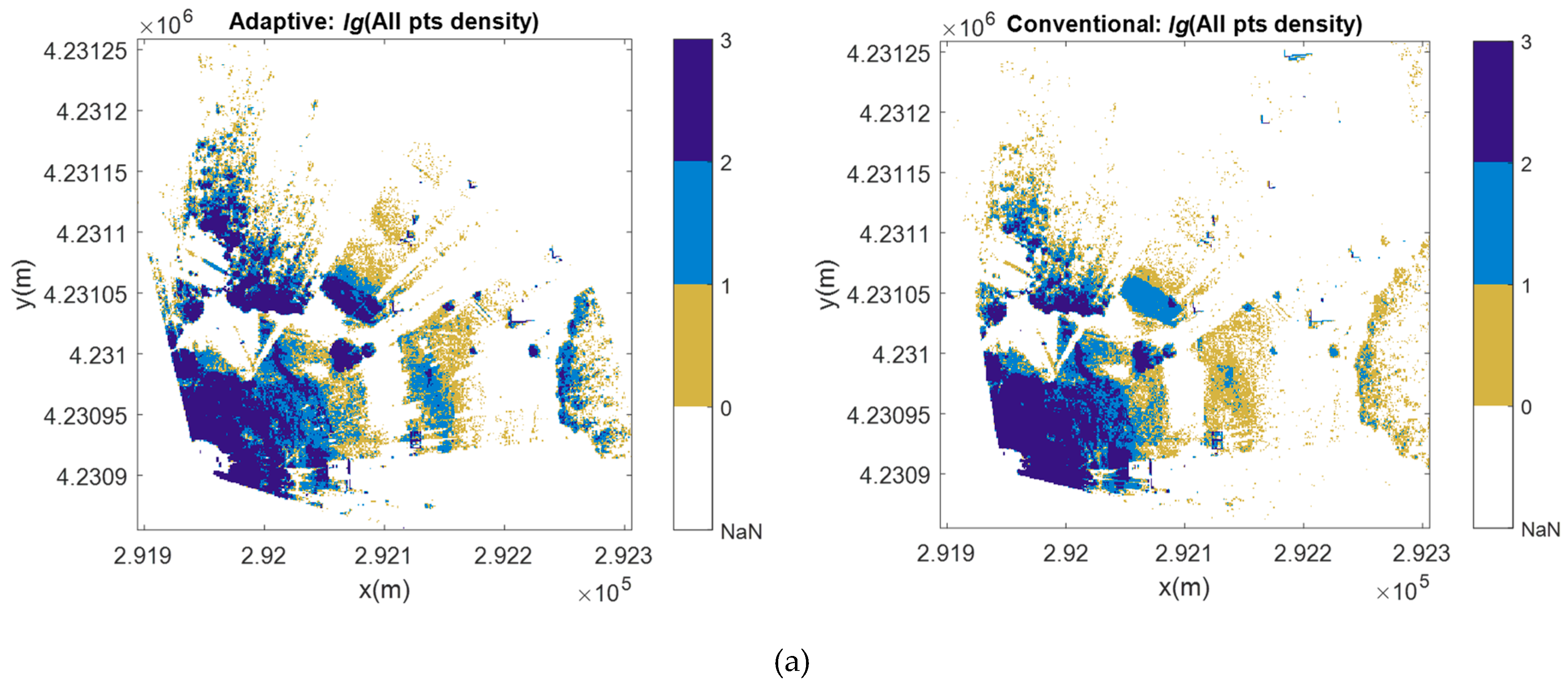
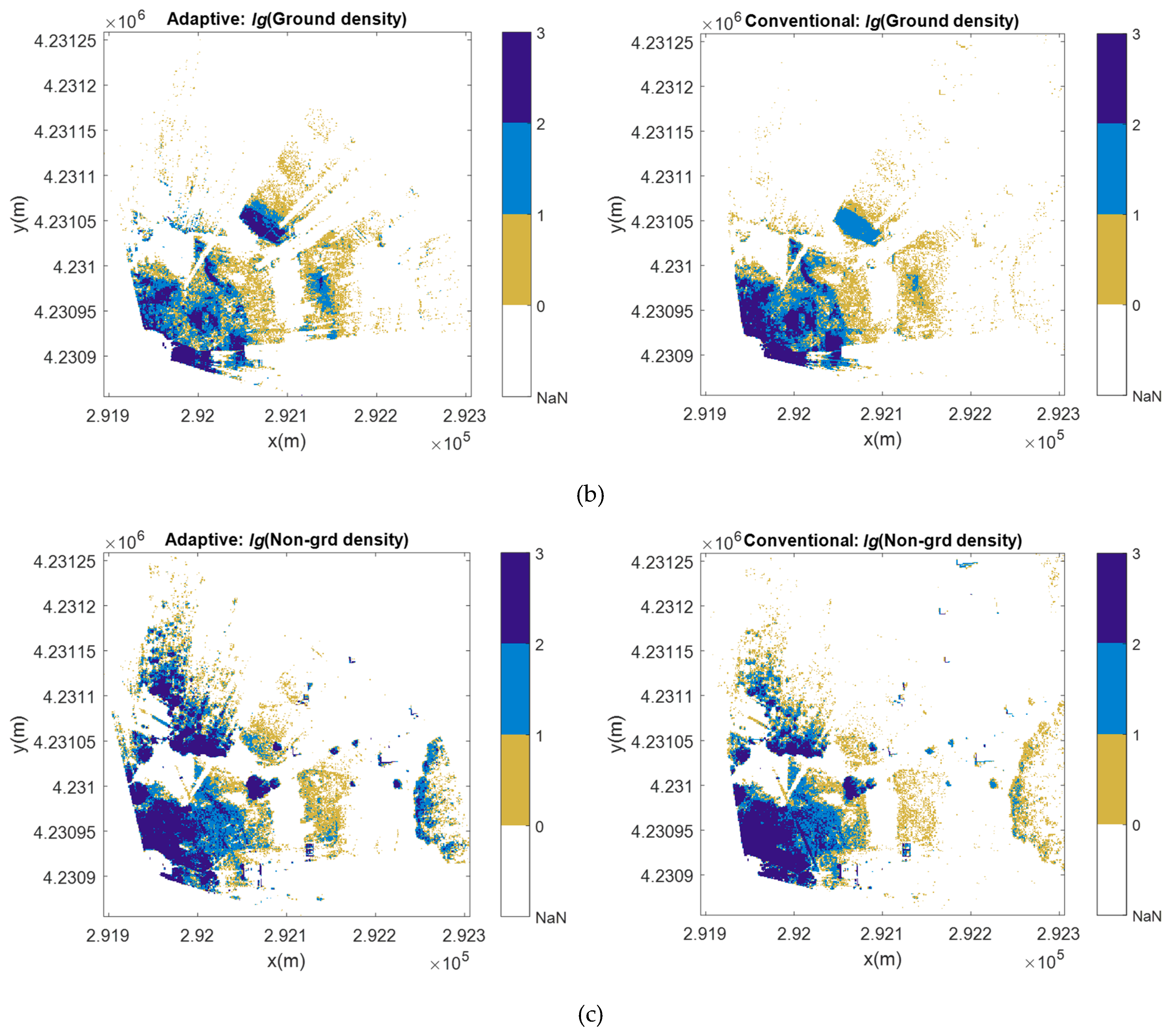
The study area was divided into 1 × 1 m2 grids and the number of points in each grid was counted. The results in logarithmic scale are plotted in Figure 6a–c, respectively for all points, ground points, and nonground points. We compare the results side by side in Figure 6 for the two scanning modes.
For areas closest to the scanner (i.e., the lower left section of the plots), the conventional mode generated clearly more points or higher point density than the adaptive mode did. According to several previous studies concluded in [9,12], a point density exceeding a certain threshold makes little additional contribution to subsequent information extraction. Their research has found that more than 16 points per square meter (points/m2) for building boundary extraction and more than 5 points/m2 for forest biomass estimation represent such thresholds [9,12]. As such, it is practically meaningful and beneficial to suppress the sampling rate in areas closer to the scanner. In the same time, for regions distant from the scanner, adaptive scanning at a minimum point density of 10 points/m2 could cover more places than the conventional mode did. Furthermore, many distant places with a point density less than 10 points/m2 (logarithmic value < 1) in the conventional scan could be sampled with a higher density by the adaptive scanning. Per definition of its design, the adaptive sampling method is indeed in favor of the distant targets. Without this necessary denser sampling, the point cloud collected in the conventional mode may not easily meet the minimum requirement in many critical applications.
Figure 6b shows the distribution of the ground points and Figure 6c the non-ground points. Similar discussions can be made for these classified groups. In either of the two separated point clouds, locations closer to the scanner were more than necessarily over-sampled at 100 points/m2 or higher (logarithmic value ≥ 2), whereas many distant objects were under-sampled with less than 10 points/m2 (logarithmic value < 1). The adaptive scanning clearly reached a better and balanced sampling as desired and could cover the entire scene at a satisfactory density with fewer amount of total data (Table 3).
4.3. Spectral Analysis
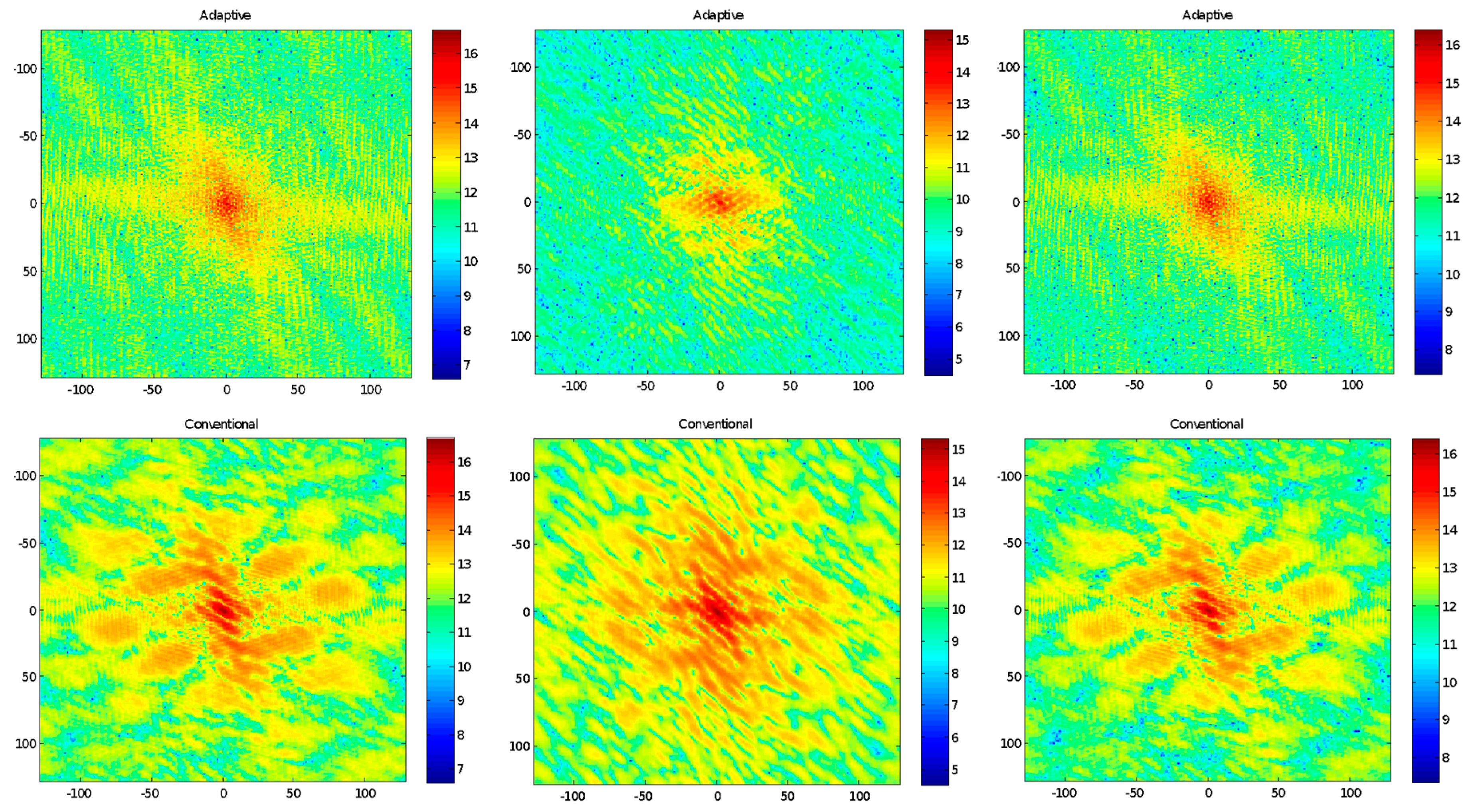
Point density can also be examined in frequency domain. We conducted a 2-D Fourier transformation on the point distribution with
where p and q are indices of the 2-D Fourier transformation, d is the point density at the grid (j + 1, k + 1), M = 256 and N = 256 in this study. The results were then shifted so that the frequency responses are centered at the “zero” frequencies. Ideally, if the lidar points are evenly distributed over the entire study area, a single peak in the 2-D spectrum would be expected. In the experiment, as is shown in Figure 7, the point density of the adaptive scanning is mostly concentrated at the center of the plots, whereas the point density of the conventional scanning has a wide spread over all frequencies. This occurs to all three groups of point clouds: all points, ground points, and nonground points, suggesting less uniform distribution in the spatial domain.
5. Point Density on Selected Objects
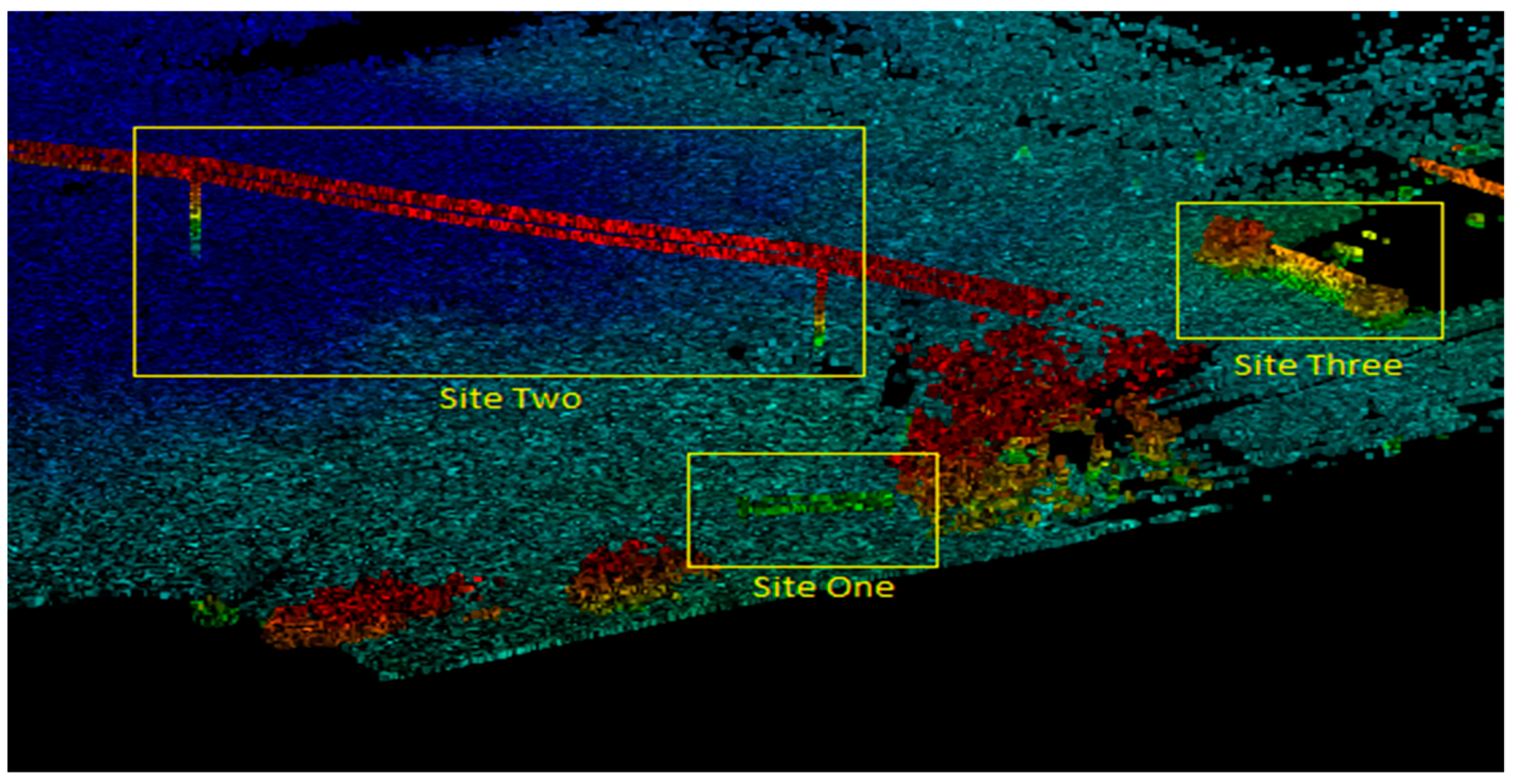
This section will evaluate the point density on objects (targets) in the adaptive point clouds as a comparison to the conventional point clouds. To this end, we selected a few representative objects in the datasets, namely two sites of electric poles and power lines, and one site of a building.
5.1. Electric Poles and Power Lines
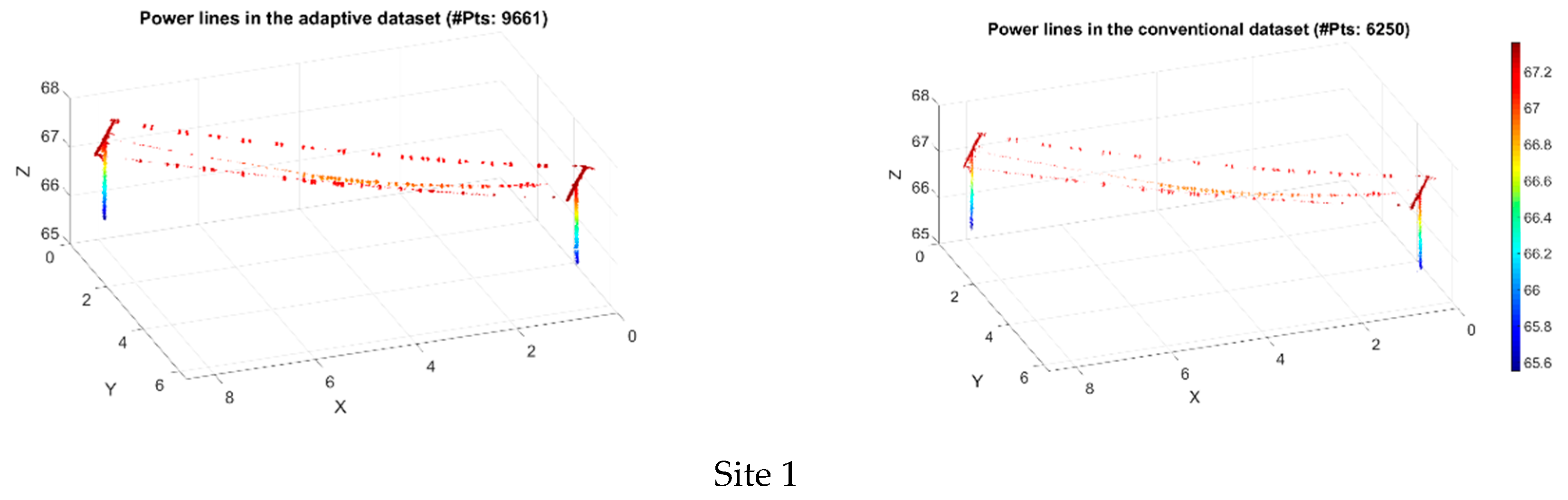
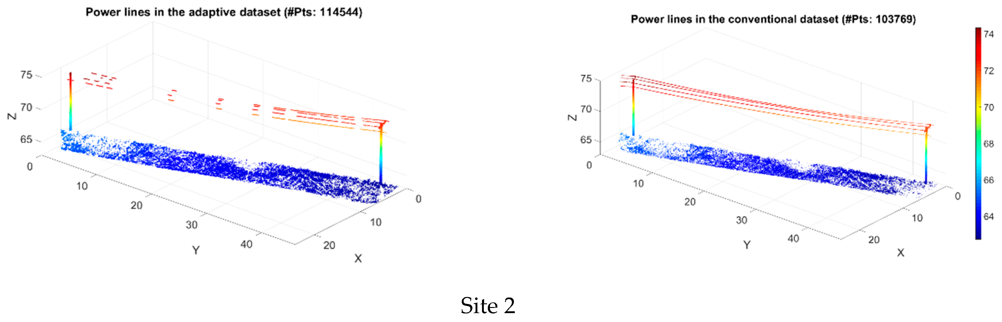
We chose two sites of electric poles and power lines in both the adaptive dataset and the conventional dataset. They are representatives of isolated linear objects. Both sites are in close range (see Figure 8): Site 1 is about 54 m to the scanner, while Site 2 is about 77 m away. Point clouds at Site 1 contain only points of electric poles and power lines, while point clouds of Site 2 include poles and power lines as well as some ground points.
For each dataset, we divided its point clouds into 10 vertical layers with equal height interval. They are labeled as 1 to 10 from ground to the top of the objects. The height intervals in Site 1 and Site 2 are 0.18 m and 1.14 m, respectively. The number of points in each layer is shown in Table 4, where shaded cells are the layers that have more points in conventional mode than in the adaptive mode.
It is noticed from Table 4 that the adaptive point cloud has more points than the conventional mode in all layers in Site 1 and most of the layers in Site 2. The only exception is layer 1, 2, 9, and 10 in Site 2 (shaded in Table 4). In Site 2, Layer 1 and 2 contain part of the ground points, where the conventional point cloud has nearly 10% more points than the adaptive point cloud dataset. The fact that conventional point cloud dataset has higher point density in Layer 1 and 2 was also illustrated in Figure 6b.
The middle layers, from Layer 3 to 8, are mostly for the poles in both Site 1 and Site 2. Table 4 and Figure 9 demonstrate the adaptive point cloud has higher point density than the counterparts of the conventional point cloud. This suggests that the adaptive mode can reach a better performance in scanning vertical objects, outperforming the conventional mode even in near range (0–100 m). Meanwhile, since Site 2 is farther away than Site 1 and the ratios (A/C) of layer 3–8 in Site 2 are higher than the ratios (A/C) of layer 3–8 in Site 1, we conclude that the adaptive mode can keep its capability to scan vertical objects at distance.
Figure 9 also reveals that the power lines in Site 2 were more completely recorded in the conventional dataset than in the adaptive dataset. The adaptive dataset even has significant missing data. As discussed earlier, the adaptive mode adjusts its pulse repetition rate based on the zoning results from an initial overview scan. Small, isolated objects, such as segments of the power lines in this case, could be missed due to the low pulse repetition rate used in the overview scan. Consequently, the subsequent fine scanning would not be effectively targeted to the areas where objects were not detected during the initial overview scan. Therefore, if small objects (often isolated from their neighbors in vertical direction) are missed during the overview scan, it may be missed either partly or completely during the adaptive scanning, resulting in incomplete data collections.
Conversely, the opposite phenomenon can be observed for objects at distance. Figure 10 labels two electric poles in the region about 300 m from the scanner. In the adaptive dataset, the electric poles (in the yellow rectangles), as well as other vertical objects such as trees and walls, are more visible than the ones in the conventional mode, which are hard to distinguish. It demonstrates that adaptive scanning, which scans distant objects at a higher pulse repetition rate, could capture objects with a higher density than the conventional dataset. This is more obvious and critical for isolated vertical objects.
5.2. Building Structures—Walls
We chose a wall located at Site 3 (Figure 8) about 106 m from the scanner. The wall is rendered differently in the adaptive dataset (Figure 11a) as compared to the conventional dataset (Figure 11b). As shown by the red boxes in Figure 11a and b, we further examined a rectangular region of 1 m × 4 m on the wall. The region was divided into grids of 0.1 m × 0.1 m. As shown in Figure 11c and d, the point density on the wall in the adaptive dataset is significantly higher than the conventional one (300 points/m2 versus 45 points/m2). The median point density of the wall in the adaptive dataset is about 150 points/m2, whereas the median point density in the conventional dataset is less than 30 points/m2. Figure 11d reveals some vertical strips periodically appearing on the wall, demonstrating the vertical scanning pattern of the mirror while the scanner was rotating. Such a vertical striping pattern is not apparently visible in the adaptive point cloud dataset (Figure 11c). Although the point density on the wall in the adaptive dataset is high, it is less uniform than the conventional dataset due to the overlap between the adaptive zones.
As shown in Figure 11, the place where the blue “^” pattern (see Figure 11a red box and 11c point density) appears at the bottom right of the adaptive dataset is actually at the boundary between two zones. Part of the wall was scanned twice, yielding higher point density in the final coverage (Figure 11c) than either of the two scans alone. The combination of the two plots in Figure 12 produces Figure 11c. This observation is consistent with the design schema that the scan zones have a small overlap (in range as well as angle) to ensure that there are no gaps between zones. However, this would result in some areas being scanned twice.
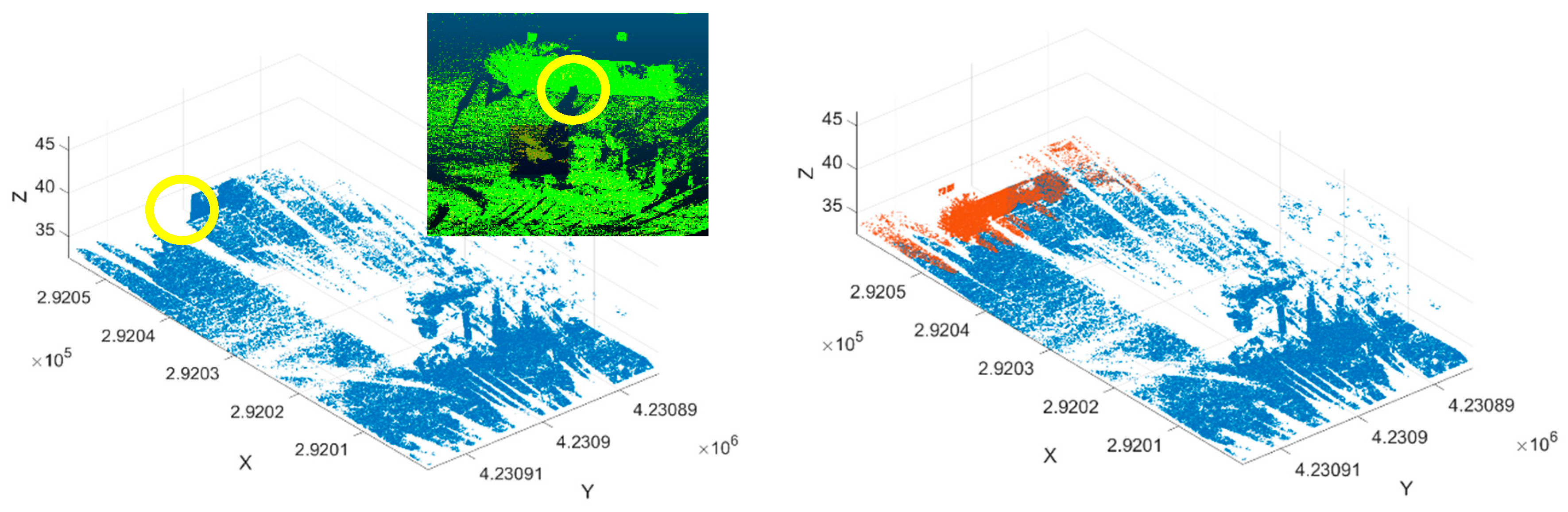
There is also another example of missing targets other than duplication for the adaptive scanning. A small void (dark) area (Figure 11a) can be observed in the middle bottom of the adaptive dataset which does not exist in the conventional dataset. As shown in Figure 13, this is due to a bush located in front of the wall. The bush has influenced both the conventional dataset and adaptive one since part of the ground behind the bush was missing due to the laser shadow. However, the influence on the adaptive dataset is worse as part of the wall was missing as well. As we discussed before, the scanner in the adaptive mode adapts pulse repetition rate according to the zones generated from initial overview scan. The wall and its surrounding are mostly in zone 2 and 3. It is likely that the initial overview scan detected the bush as the only target in this direction. When scanning zone 2, the scanner used a pulse repetition rate that was unable to “penetrate” the foliage of the bush. Therefore, in Figure 13 only part of the wall was detected. When scanning zone 3, the scanner returned nothing at the place behind the bush, resulting in the occlusion of the wall. Contrary to this, the conventional mode scans the whole scene ‘blindly’ at a constant pulse repetition rate, which eventually “penetrates” the bush and reaches the wall behind it. As a result, the points on the wall in the conventional dataset are more uniform and complete (see Figure 11).
6. Conclusions
We conducted a comparative evaluation between adaptive scanning and conventional scanning methodologies under the scope of point densities in topographic laser scanning. The adaptive scanner HRS3D-AS prototype was designed and developed to achieve an ideal uniform point density over the entire scene. It accomplishes this by adjusting its pulse repetition rate and angular resolution with respect to the zones of distances to the scanner determined during an initial overview scan. Overall, our study reveals that the adaptive scanner is capable to produce more evenly distributed point clouds. Objects distant from the scanner are more uniformly and more densely recorded than the conventional scanning does. In the meantime, the point density for objects closer to the scanner is still acceptable and not as unnecessarily high as in the conventional scanning. Moreover, the total data volume generated under the adaptive scanning is less than or equivalent to the conventional scanning. As a result, the adaptive scanning is feasible and can be achieved with a more uniformed point density across the scene with less total data amount than the conventional scanning. We have demonstrated these properties by analyzing the distribution of point density with respect to the 1-D distance to the scanner, 2-D spatial locations in the scene, and by carrying out a spectral analysis for the point density.
However, the adaptive scanning method is not yet a perfect practical implementation. Although the overall point density is more even than the conventional scanning, places at zone boundaries sometimes may demonstrate significant density variation. This is due to the duplicated coverage at the zone boundary, i.e., they are scanned at least twice under different point densities, yielding large density variations comparing to places that are only scanned once. Another concern, which might be more critical, is the unexpected void in the adaptive scanning. Since the initial overview scan is used to detect objects and decide the pulse repetition rates to be used for the subsequent scanning, an improper initial overview scan may miss small, isolated objects in the scene. It can also produce scans too coarse to ‘penetrate’ foliage of trees or bushes such that occlusion occurs where objects occurring behind are not rendered by the scanner, leading to gaps or voids in a dataset.
Both duplication and missing data in adaptive scanning could be problematic in subsequent data processing. Although the adaptive scanning achieves overall even density in the scene, the unevenness of point density at zone boundaries can cause difficulties in a number of point cloud data processing tasks, such as ground filtering, object segmentation, object recognition and object reconstruction. Similarly, voids or gaps will lead to mistakes and insufficient sampling or incomplete object detection and reconstruction. Our study suggests that the zone information or the zone ID associated with the point cloud files would be helpful for data processing. Similarly, adaptive scanning practice should be improved to assure minimum overlap at zone boundaries and in the same time to avoid scan voids or gaps due to inappropriate overview scan. This is a challenge for improvement in the scanner design, functionality enhancement, and eventual manufacture as well.
Author Contributions
Conceptualization: J.A. and J.C.; methodology: Q.L., J.S.; software: Q.L. and Y.M.; validation: Q.L. and Y.M.; formal analysis and investigation: Q.L., Y.M., J.A., J.C., J.S.; resources: J.A., J.C., J.S.; data curation: J.A., J.C.; writing—original draft preparation: Q.L., Y.M., J.S.; writing—review and editing: Q.L., Y.M., J.A., J.C., J.S.; supervision: J.S.
Funding
The work was supported in part by the Army Research Office.
Conflicts of Interest
The authors declare no conflicts of interest.
References
- Petrie, G.; Toth, C. Introduction to Laser Ranging, Profiling, and Scanning, Chapter 1. In Topographic Laser Ranging and Scanning: Principles and Processing, 2nd ed.; Shan, J., Toth, C.K., Eds.; CRC Press: Boca Raton, FL, USA, 2018. [Google Scholar]
- Heidemann, H.K. Lidar Base Specification Version 1.0. (USGS Techniques and Methods 11-B4); US Geological Survey: Reston, VA, USA, 2012.
- Williams, K.; Olsen, M.J.; Roe, G.V.; Glennie, C. Synthesis of transportation applications of mobile LiDAR. Remote Sens. 2013, 5, 4652–4692. [Google Scholar] [CrossRef]
- Wulf, O.; Wagner, B. Fast 3D scanning methods for laser measurement systems. Int. Conf. Control. Syst. Comput. Sci. 2003, 25, 1–14. [Google Scholar]
- Morales, J.; Plazaleiva, V.; Mandow, A.; Gomezruiz, J.A.; Serón, J.; Garcíacerezo, A. Analysis of 3d scan measurement distribution with application to a multi-beam lidar on a rotating platform. Sensors 2018, 18, 395. [Google Scholar] [CrossRef] [PubMed]
- Roussel, J.R.; Caspersen, J.; Béland, M.; Thomas, S.; Achim, A. Removing bias from LiDAR-based estimates of canopy height: Accounting for the effects of pulse density and footprint size. Remote Sens. Environ. 2017, 198, 1–16. [Google Scholar] [CrossRef]
- Singh, K.K.; Chen, G.; McCarter, J.B.; Meentemeyer, R.K. Effects of LiDAR point density and landscape context on estimates of urban forest biomass. ISPRS J. Photogramm. Remote Sens. 2015, 101, 310–322. [Google Scholar] [CrossRef]
- Singh, K.K.; Chen, G.; Vogler, J.B.; Meentemeyer, R.K. When big data are too much: Effects of LiDAR returns and point density on estimation of forest biomass. IEEE J. Sel. Top. Appl. Earth Obs. Remote Sens. 2016, 9, 3210–3218. [Google Scholar] [CrossRef]
- Garcia, M.; Saatchi, S.; Ferraz, A.; Silva, C.A.; Ustin, S.; Koltunov, A.; Balzter, H. Impact of data model and point density on aboveground forest biomass estimation from airborne LiDAR. Carbon Balance Manag. 2017, 12, 4. [Google Scholar] [CrossRef] [PubMed] [Green Version]
- Kandare, K.; Ørka, H.O.; Chan, J.C.W.; Dalponte, M. Effects of forest structure and airborne laser scanning point cloud density on 3D delineation of individual tree crowns. Eur. J. Remote Sens. 2016, 49, 337–359. [Google Scholar] [CrossRef] [Green Version]
- Jakubowski, M.K.; Guo, Q.; Kelly, M. Tradeoffs between lidar pulse density and forest measurement accuracy. Remote Sens. Environ. 2013, 130, 245–253. [Google Scholar] [CrossRef]
- Tomljenovic, I.; Rousell, A. Influence of point cloud density on the results of automated Object-Based building extraction from ALS data. In Proceedings of the 17th AGILE Conference on Geographic Information Science, Castellon, Spain, 3–6 June 2014. [Google Scholar]
- Rozas, E.; Rivera, F.F.; Cabaleiro, J.C.; Pena, T.F.; Vilariño, D.L. Comparative study of building footprint estimation methods from LiDAR point clouds. In Proceedings of the Image and Signal Processing for Remote Sensing XXIII, Warsaw, Poland, 11–13 September 2017; Volume 10427, p. 104270R. [Google Scholar]
- Cahalane, C.; McElhinney, C.P.; Lewis, P.; McCarthy, T. MIMIC: An innovative methodology for determining mobile laser scanning system point density. Remote Sens. 2014, 6, 7857–7877. [Google Scholar] [CrossRef]
- Kodors, S. Point Distribution as True Quality of LiDAR Point Cloud. Balt. J. Mod. Comput. 2017, 5, 362–378. [Google Scholar] [CrossRef]
- Mandow, A.; Martínez, J.L.; Reina, A.J.; Morales, J. Fast range-independent spherical subsampling of 3D laser scanner points and data reduction performance evaluation for scene registration. Pattern Recognit. Lett. 2010, 31, 1239–1250. [Google Scholar] [CrossRef]
- Rusu, R.B.; Blodow, N.; Marton, Z.C.; Beetz, M. Aligning point cloud views using persistent feature histograms. In Proceedings of the 2008 IEEE/RSJ International Conference on Intelligent Robots and Systems, Nice, France, 22–26 September 2008; pp. 3384–3391. [Google Scholar]
- Pomerleau, F.; Colas, F.; Siegwart, R. A review of point cloud registration algorithms for mobile robotics. Found. Trends Robot. 2015, 4, 1–104. [Google Scholar] [CrossRef]
- Rusu, R.B.; Blodow, N.; Beetz, M. Fast point feature histograms (FPFH) for 3D registration. In Proceedings of the 2009 IEEE International Conference on Robotics and Automation, Kobe, Japan, 12–17 May 2009; pp. 3212–3217. [Google Scholar]
- Alismail, H.; Browning, B. Automatic calibration of spinning actuated lidar internal parameters. J. Field Robot. 2015, 32, 723–747. [Google Scholar] [CrossRef]
- Hackel, T.; Wegner, J.D.; Schindler, K. Fast semantic segmentation of 3d point clouds with strongly varying density. ISPRS Annals of Photogrammetry. Remote Sens. Spat. Inf. Sci. 2016, 3, 177–184. [Google Scholar]
- Grilli, E.; Menna, F.; Remondino, F. A review of point clouds segmentation and classification algorithms. Int. Arch. Photogramm. Remote Sens. Spatial Inf. Sci. 2017, 42, W3. [Google Scholar]
- Zhu, Q.; Li, Y.; Hu, H.; Wu, B. Robust point cloud classification based on multi-level semantic relationships for urban scenes. ISPRS J. Photogramm. Remote Sens. 2017, 129, 86–102. [Google Scholar] [CrossRef]
- Neumann, T.; Dülberg, E.; Schiffer, S.; Ferrein, A. A Rotating Platform for Swift Acquisition of Dense 3D Point Clouds. In International Conference on Intelligent Robotics and Applications; Springer: Cham, Switzerland, 2016; pp. 257–268. [Google Scholar]
- Berglund, J.; Lindskog, E.; Johansson, B. On the trade-off between data density and data capture duration in 3D laser scanning for production system engineering. Procedia CIRP 2016, 41, 697–701. [Google Scholar] [CrossRef]
- Massaro, R.D.; Anderson, J.E.; Nelson, J.D.; Edwards, J.D. A comparative study between frequency-modulated continuous wave LADAR and linear LiDAR. The International Archives of Photogrammetry. Remote Sens. Spat. Inf. Sci. 2014, 40, 233. [Google Scholar]
- Anderson, J.; Massaro, R.; Curry, J.; Reibel, R.; Nelson, J.; Edwards, J. LADAR: Frequency-Modulated, Continuous Wave LAser Detection and Ranging. Photogramm. Eng. Remote Sens. 2017, 83, 721–727. [Google Scholar] [CrossRef]
Figure 1.
Illustration of the adaptive scanning principle for HRS3D-AS.

Figure 2.
The study area at the National Oceanic and Atmospheric Administration’s (NOAA) site in Corbin, Virginia, USA showing an overview image (left) and recent natural color orthophotograph acquired in 2017 (right).
Figure 2.
The study area at the National Oceanic and Atmospheric Administration’s (NOAA) site in Corbin, Virginia, USA showing an overview image (left) and recent natural color orthophotograph acquired in 2017 (right).

Figure 3.
Point clouds were acquired by the HDS3S-AS using (a) a deployable 6 m high tower for the scanner. Also shown are (b) the scan origin and region designated by white arrows and a resulting scan in (c) using white to highlight conventional scanning, and blue to highlight the adaptive scan regions. It is noticeable that most parts of these two-point clouds are overlapping while the range of the point cloud by conventional mode is much further.

Figure 4.
Zone determination for the adaptive scanning. (a) The distances to the sensor (top), horizontal (middle) and vertical (bottom) angles of the adaptive lidar points in the order of their acquisition; (b) points of five zones determined from the combined point cloud file; and (c) points shown by their seven separate zone files.

Figure 5.
Number of lidar points (left column) and their density (right column) as a function of distance to scanner for ground points (a and b) and non-ground points (c and d).
Figure 5.
Number of lidar points (left column) and their density (right column) as a function of distance to scanner for ground points (a and b) and non-ground points (c and d).

Figure 6.
Logarithmic point density distribution for adaptive and conventional scanning modes. (a). All points from adaptive (left) and conventional (right) modes; (b). Ground points from adaptive (left) and conventional (right) modes; (c). Non-ground points from adaptive (left) and conventional (right) modes.


Figure 7.
2-D Fourier transform of the point density for adaptive scanning (top) and conventional scanning (bottom), with the left column for all points, the middle column for ground points, and the right column for non-ground points.
Figure 7.
2-D Fourier transform of the point density for adaptive scanning (top) and conventional scanning (bottom), with the left column for all points, the middle column for ground points, and the right column for non-ground points.

Figure 8.
Selected study sites in the adaptive point clouds.

Figure 9.
Point clouds of two sites of power lines from adaptive (left) and conventional scanning (right). (Shift: −291996.01 m, −4230895.64 m).
Figure 9.
Point clouds of two sites of power lines from adaptive (left) and conventional scanning (right). (Shift: −291996.01 m, −4230895.64 m).


Figure 10.
Electric poles (two rectangles) and vertical objects at distant (~300 m). (left: adaptive mode, right: conventional mode).
Figure 10.
Electric poles (two rectangles) and vertical objects at distant (~300 m). (left: adaptive mode, right: conventional mode).

Figure 11.
The point clouds (a,b) of a wall and their point densities (c,d) shown for a selected region on the wall for the adaptive (left) and conventional (right) datasets. The size of each grid is 0.1 m × 0.1 m. Notice the blue “^” region in (c) has lower scan density than its neighbors. “.
Figure 11.
The point clouds (a,b) of a wall and their point densities (c,d) shown for a selected region on the wall for the adaptive (left) and conventional (right) datasets. The size of each grid is 0.1 m × 0.1 m. Notice the blue “^” region in (c) has lower scan density than its neighbors. “.

Figure 12.
Point density on the wall of the adaptive dataset from zone 2 (left) and zone 3 (right). The size of each cell is 0.1 m × 0.1 m.
Figure 12.
Point density on the wall of the adaptive dataset from zone 2 (left) and zone 3 (right). The size of each cell is 0.1 m × 0.1 m.

Figure 13.
Part of the wall (circled) is occluded by a bush in the adaptive scan. Left: zone 2 plot (blue) with an inset showing an overview. Right: zone 3 (red) plotted above zone 2.
Figure 13.
Part of the wall (circled) is occluded by a bush in the adaptive scan. Left: zone 2 plot (blue) with an inset showing an overview. Right: zone 3 (red) plotted above zone 2.


Table 1.
Specifications of the HRS3D-AS scanner.
| Manufacturer | Blackmore |
|---|---|
| Model | HRS3D-AS |
| Laser Class | IIIb |
| Wavelength | 1550 nm |
| Beam divergence | 0.1 mrad |
| Horizontal field-of-view (FOV) | 360° |
| Horizontal Resolution | 0.001° |
| Vertical field-of-view (FOV) | 60° (−30° ~ +30°) |
| Vertical Resolution | 0.001° |
| Pulse (Measurement) repetition rate | up to 48 kHz |
| Laser/detector pairs | 1 |
| Range | 2400 m |
| Accuracy (at 100 m) | 10mm (1-sigma range noise) |
| Data Type | Distance/Calibrated reflectivity* |
| Size (L × W × H) | (11.1” × 14.2” × 21.7”) |
* Distance/Calibrated Reflectivity refers to the process we use to range-normalize intensity returns from the sensor. Reflectivity values are reported out on a zero-to-one scale, where 0 represents 0% reflectivity and 1.0 represents 100% diffuse reflectivity. Reflectivity values greater than 1.0 are reported for retroreflective objects.
Table 2.
Zone designation of the HRS3D-AS scanner under its adaptive mode.
| Zone ID | Range (m) | Frequency | Zone ID | Range (m) | Frequency |
|---|---|---|---|---|---|
| 1 | 0–50 | 48 kHz | 7 | 300–350 | 12 kHz |
| 2 | 50–100 | 24 | 8 | 350–400 | 12 |
| 3 | 100–150 | 24 | 9 | 400–600 | 12 |
| 4 | 150–200 | 12 | 10 | 600–1000 | 6 |
| 5 | 200–250 | 12 | 11 | 1000–1500 | 6 |
| 6 | 250–300 | 12 | 12 | 1500–2400 | 3 |
Table 3.
Summary of data collections with HDS3D-AS scanner under adaptive and conventional modes at Corbin, VA.
Table 3.
Summary of data collections with HDS3D-AS scanner under adaptive and conventional modes at Corbin, VA.
| Adaptive | Conventional | |
|---|---|---|
| UTM Zone | 18 N | 18 N |
| Scanner location (est’ed) | X = 291,946, Y = 4,230,903 | X = 291,947.5, Y = 4,230,902 |
| X range | 291,894.3–292,305.9 | 291,889.5–292,532.3 |
| Y range | 4,230,855.2–4,231,258.7 | 4,230,828.1–4,231,404.5 |
| Z range | 59.8–85.4 | 60.2–81.1 |
| # of points | 14,122,242 | 17,924,721 |
| # of ground points | 1,800,755 | 4,545,200 |
| # of non-ground points | 12,321,487 | 13,379,521 |
Table 4.
Number of lidar points in vertical layers for Site 1 and Site 2 (shown in Figure 8) from adaptive (A) and conventional scanning (C). The four highlighted cells are the cases where the adaptive scanning yields fewer data than the conventional scanning does.
Table 4.
Number of lidar points in vertical layers for Site 1 and Site 2 (shown in Figure 8) from adaptive (A) and conventional scanning (C). The four highlighted cells are the cases where the adaptive scanning yields fewer data than the conventional scanning does.
| Layer # | # Points in Site 1 | # Points in Site 2 | ||||
|---|---|---|---|---|---|---|
| A | C | A/C | A | C | A/C | |
| 1 | 150 | 139 | 1.0791 | 31522 | 34005 | 0.9270 |
| 2 | 248 | 214 | 1.1589 | 23061 | 25843 | 0.8923 |
| 3 | 275 | 208 | 1.3221 | 7110 | 3913 | 1.8170 |
| 4 | 327 | 218 | 1.5000 | 7642 | 3525 | 2.1679 |
| 5 | 304 | 222 | 1.3694 | 7260 | 3328 | 2.1815 |
| 6 | 286 | 205 | 1.3951 | 7044 | 3294 | 2.1384 |
| 7 | 297 | 191 | 1.5550 | 6857 | 3135 | 2.1872 |
| 8 | 1553 | 879 | 1.7668 | 8021 | 5806 | 1.3815 |
| 9 | 2114 | 1020 | 2.0725 | 10997 | 13127 | 0.8377 |
| 10 | 4107 | 2954 | 1.3903 | 5030 | 7793 | 0.6455 |
| Total | 9661 | 6250 | 1.5468 | 114544 | 103769 | 1.1038 |
© 2019 by the authors. Licensee MDPI, Basel, Switzerland. This article is an open access article distributed under the terms and conditions of the Creative Commons Attribution (CC BY) license (http://creativecommons.org/licenses/by/4.0/).
Share and Cite
MDPI and ACS Style
Li, Q.; Ma, Y.; Anderson, J.; Curry, J.; Shan, J. Towards Uniform Point Density: Evaluation of an Adaptive Terrestrial Laser Scanner. Remote Sens. 2019, 11, 880. https://0-doi-org.brum.beds.ac.uk/10.3390/rs11070880
AMA Style
Li Q, Ma Y, Anderson J, Curry J, Shan J. Towards Uniform Point Density: Evaluation of an Adaptive Terrestrial Laser Scanner. Remote Sensing. 2019; 11(7):880. https://0-doi-org.brum.beds.ac.uk/10.3390/rs11070880
Chicago/Turabian StyleLi, Qinghua, Yuchi Ma, John Anderson, James Curry, and Jie Shan. 2019. "Towards Uniform Point Density: Evaluation of an Adaptive Terrestrial Laser Scanner" Remote Sensing 11, no. 7: 880. https://0-doi-org.brum.beds.ac.uk/10.3390/rs11070880
Note that from the first issue of 2016, this journal uses article numbers instead of page numbers. See further details here.