Smallholder Crop Area Mapped with a Semantic Segmentation Deep Learning Method


1
College of Land Science and Technology, China Agricultural University, Beijing 100083, China
2
Key Laboratory of Agricultural Land Quality, Ministry of Land and Resources of the China, Beijing 100083, China
*
Author to whom correspondence should be addressed.
Remote Sens. 2019, 11(7), 888; https://0-doi-org.brum.beds.ac.uk/10.3390/rs11070888
Submission received: 19 February 2019
/
Revised: 2 April 2019
/
Accepted: 3 April 2019
/
Published: 11 April 2019
(This article belongs to the Special Issue Earth Observations and Crop Models for Sustainable Agricultural Management)
Abstract
:The growing population in China has led to an increasing importance of crop area (CA) protection. A powerful tool for acquiring accurate and up-to-date CA maps is automatic mapping using information extracted from high spatial resolution remote sensing (RS) images. RS image information extraction includes feature classification, which is a long-standing research issue in the RS community. Emerging deep learning techniques, such as the deep semantic segmentation network technique, are effective methods to automatically discover relevant contextual features and get better image classification results. In this study, we exploited deep semantic segmentation networks to classify and extract CA from high-resolution RS images. WorldView-2 (WV-2) images with only Red-Green-Blue (RGB) bands were used to confirm the effectiveness of the proposed semantic classification framework for information extraction and the CA mapping task. Specifically, we used the deep learning framework TensorFlow to construct a platform for sampling, training, testing, and classifying to extract and map CA on the basis of DeepLabv3+. By leveraging per-pixel and random sample point accuracy evaluation methods, we conclude that the proposed approach can efficiently obtain acceptable accuracy (Overall Accuracy = 95%, Kappa = 0.90) of CA classification in the study area, and the approach performs better than other deep semantic segmentation networks (U-Net/PspNet/SegNet/DeepLabv2) and traditional machine learning methods, such as Maximum Likelihood (ML), Support Vector Machine (SVM), and RF (Random Forest). Furthermore, the proposed approach is highly scalable for the variety of crop types in a crop area. Overall, the proposed approach can train a precise and effective model that is capable of adequately describing the small, irregular fields of smallholder agriculture and handling the great level of details in RGB high spatial resolution images.
1. Introduction
The demand for agricultural production is increasing all over the world as a result of the growing global population. The food consumed annually by China alone has increased significantly over the past decades [1]. China has one of the largest populations in the world, and it is currently undergoing rapid urbanization. The continually increasing population and decreasing crop area (CA) highlight the necessity of CA protection. As an effective way to protect CA and determine CA changes, classification through remote sensing (RS) has been utilized to monitor the spatial distribution of agriculture and provide basic data for crop growth monitoring and yield forecasting, particularly for smallholder family farming in China [2,3,4,5].
Smallholder family farming is characterized by family-focused motives, such as favoring the stability of the farm household system; it mainly employs family labor for production and uses part of the farm’s products for the family’s consumption [6]. CA in this system is usually characterized by small, heterogeneous, and often indistinct field patterns. Almost 70–80% of food in China is provided by this system [7]. These fields are smaller than 2 ha, which makes resolving their distribution difficult with moderate spatial resolution (30–500 m) satellite imagery. The small size and large distribution area of smallholder family farming highlight the need for a precise and automatic method to map CA via high spatial resolution remote sensing images.
However, previous studies on CA or land cover maps in China and around the world have been mostly based on medium or low spatial resolution images [8,9]. At the coarse scale (>= 500 m), using the decision tree method and Moderate Resolution Imaging Spectroradiometer (MODIS), Friedl et al. [10] and Tateishi et al. [11] finished the global land cover classification task. With the openness of Landsat series images and the development of Google Earth Engine (GEE), a number of different approaches have been applied at the moderate resolution scale (30–500 m) [12,13,14,15,16]. For medium-high resolution (10–30 m) satellites, because of its high spatial, spectral and temporal resolution, Sentinel-2 (S2) data has been used extensively in land cover mappings [17,18], crop type classifications [19,20], and monitoring of vegetation biomass [21,22]. These studies are usually based on S2’s time series information to get better results, which results in a high cost of image preprocessing work, including cloud masking, temporal gap filling and super resolution. Recent technologies have further increased the spatial resolution of available RS images (2 m spatial resolution and higher). The rich shape and context information provided by the high spatial resolution RS images allows researchers to get precise classification results with only one single-phase RS images. There have been some studies on urban land cover classification that used high spatial resolution images [23,24], but the methods have seldom aimed to map CA at a 1 m or even higher resolution. The era of using high spatial resolution RS images for mapping very small agriculture fields has only recently materialized [25].
A high spatial resolution RS image provides the details necessary to observe smallholder agriculture. However, its low spectral resolution also presents challenges in smart image interpretation for CA to the remote sensing community. Some kinds of high spatial resolution RS images have only three bands, red-green-blue (RGB), thus lacking some useful spectral information, such as the near-infrared (NIR) band, for CA classification. Although there is vast literature on the automatic mapping of CA using machine learning algorithms, such as the inverse distance weighted interpolation method [26], decision tree [6], Support Vector Machine [27], and artificial neural network [28], the approaches have usually considered the spectrum of every individual pixel and then assigned each of them to a certain class [25].
However, contextual features have proven to be very useful for classification [29], especially when it comes to small and irregularly shaped targets. Meanwhile, the most prominent advantage of high spatial resolution RS images is their rich spatial information, so it is important to take full advantage of its contextual and shape features. Although some researchers have used texture statistics [30,31], mathematical morphology [32,33], and rotation invariance [34,35] as spatial and shape features, these mid-level features cannot describe the rich contextual information offered by high spatial resolution RS images. Moreover, these methods mostly rely on hand-engineered features, and most appearance descriptors depend on a set of free parameters, which are commonly set by user experience via experimental trial-and-error or cross-validation. So, we argue that a more thorough understanding of the spatial features, such as the shape of objects, is required to aid the mapping process of small and irregularly shaped smallholder agricultural fields.
Therefore, convolutional neural networks (CNNs) [36] have attracted attention for their ability to automatically discover relevant contextual features in classification problems. CNNs, which learn the representative and discriminative features in a hierarchical manner from the data, have recently become a hotspot in the machine learning area and have been introduced to the geoscience and RS community for object detection [37,38], scene understanding [39,40], and image processing [41,42].
Recently, semantic classification tasks in remotely sensed data have also been approached by means of CNNs. In general, CNN architectures for semantic pixel-based classification use two main approaches: patch-based and pixel-to-pixel-based (end to end). At first, Patch classification was used for the task [43,44,45]. These kinds of methods commonly start with training a CNN classifier on small image patches, followed by predicting the class of the center pixel using a sliding window approach. The drawback of these approaches is that the trained network can only predict the central pixel of the input image, resulting in low classification effectiveness. Then, an end-to-end framework for pixel-based methods became more popular [46,47,48,49] for its ability to learn global context features and its high process effectiveness [50]. These frameworks are usually called semantic segmentation networks, and end-to-end usually means jointly learning a series of feature extractions from raw input data to generate a final, task-specific output. Compared with patch classification, semantic labeling-based strategies can label each pixel in the image. The network is trained to learn not only the relationships between spectral signatures and labels but also the contextual features of the whole input image.
Results from different studies have shown that both the accuracy and efficiency of end-to-end networks outperform standard patch-based strategies [51,52], suggesting that end-to-end structures are better suited for RS image classification. Recently, semantic segmentation networks, which are popular in computer vision, have been introduced to the field of RS image classification for their ability to learn both spatial and spectral information [53,54,55]. In this study, we chose the DeepLabv3+ architecture to develop a methodology because it is effective in multi-scale feature fusion and boundary description. With the proposed method, we finished the automatic mapping of CA from Satellite images with only the three RGB bands.
In the next section, we first introduce the study area and the RS data we used in this study. In Section 3, the details of our network architecture and training/classification strategies are presented. Then, we report the results of testing our semantic classification framework on WorldView-2 (WV-2) images with only RGB bands in Section 4. Different classifiers are compared with the proposed method to prove its effectiveness, and the classification results are shown in Section 5. Then, a Discussion about the strengths of the proposed method with respect to other relevant studies is given in Section 6. Finally, considerations for future work and the conclusions of the study are given in Section 7.
2. Study Area and Data
2.1. Study Area
The study area, Baodi, lies in the north of the North China Plain and south of the Yanshan Mountains, located at 117°8′–117°40′E and 39°21′–39°50′N (Figure 1). It is a part of Tianjin, China, and near Bohai Bay. Baodi occupies approximately 1450 km2 and has a population of approximately 871,300. The region is dominated by plains, with elevations between 2.5 and 3 m. The dominant land cover in Baodi is small-scale agriculture fields that cover approximately 700–800 km2, and it has been an important food production base for Beijing and Tianjin since the year 2000.
Baodi is characterized by a warm temperate semi-humid continental monsoon climate. The four seasons are distinct, and winter and summer are longer than spring and autumn. The annual average temperature is 11.6 °C. The annual precipitation is 612.5 mm, and the frost-free period is about 184 days [56]. There are a variety of soil types throughout Baodi. The northern high area is dominated by common tidal soils. The conditions are conducive to a high yield of various crops, such as grain, fruits, vegetables, and medicinal materials: the soil texture is loamy; the fertility is high; the water, fertilizer, gas, and heat are relatively coordinated; and the soil layer is thick. The middle part is mainly moist soil, and the texture is sticky. It is suitable for rice, sorghum, soybean, green onion, cotton, and hemp. The southern area has a salinized moist soil with a wide area and a short cultivation period. It is suitable for the development of freshwater aquaculture and plants for anti-salt and anti-humid crops. The eastern area is mostly of clay soil and is suitable for planting crops such as wheat, rice, and soybean [57].
The area is interesting from the perspective of method development for a number of reasons. First, the study area is an important grain and cotton production base in northern China. Second, the diversity of soil and crop types is abundant across Baodi county, and such variety can be used to evaluate the generalization ability of the method. Third, the climate and topographic conditions of Baodi are common in the North China Plain, so a method based on this area can be easily extended to other similar areas.
2.2. Data
As mentioned before, this study aims to map the CA of smallholder family farming systems via high spatial resolution RS images. To achieve this goal, we collected WorldView-2 (WV-2) images of the study area. DigitalGlobe’s WV-2 satellite sensor, launched on 8 October 2009, provides high optical resolution and high geometric accuracy of up to 0.46 m. The WV-2 sensor provides a high-resolution panchromatic band and eight multispectral bands: four standard bands (red, green, blue, and near-infrared 1) and four new bands (coastal, yellow, red edge, and near-infrared 2). The spectrum’s diversity provides users with the ability to perform mapping and monitoring applications, land-use planning, disaster relief, exploration, defense and intelligence, and visualization and simulation environments. The images of the study area that were selected for this paper were taken in the summer and autumn with minimum cloud cover and a 1.85-m resolution. The multispectral images were then fused with the panchromatic images and resampled to a 1-m resolution. As the RS images with the highest spatial resolution have a low spectral resolution, the WV-2 images used here are in true color fusion to prove the promotability and effectiveness of the proposed method.
3. Method
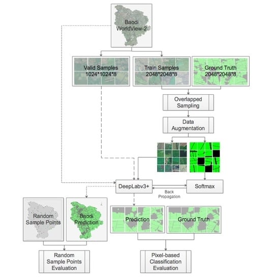
In this study, we chose DeepLabv3+ as the classification model to get the CA from the study area; the architecture of the network is presented in Section 3.1. Similar to other supervised classification methods, our approach generally has three stages (Figure 2): the training stage, the classification stage, and the accuracy evaluation stage. In the training stage, image–label pairs, with pixel-class correspondence, are input into the DeepLabv3+ network as training samples. The error between predicted class labels and ground truth (GT) labels is calculated and back-propagated through the network using the chain rule, and then the parameters of the DeepLabv3+ network are updated using the gradient descent method. In the classification stage, the trained DeepLabv3+ network is fed an input image to generate a class prediction. Then, two kinds of evaluation methods are employed in the accuracy evaluation stage to establish the effectiveness of the proposed method. The details of the training and classification stages are introduced in Section 3.2, while the two accuracy evaluation methods are detailed in Section 3.3.
3.1. Network Architecture
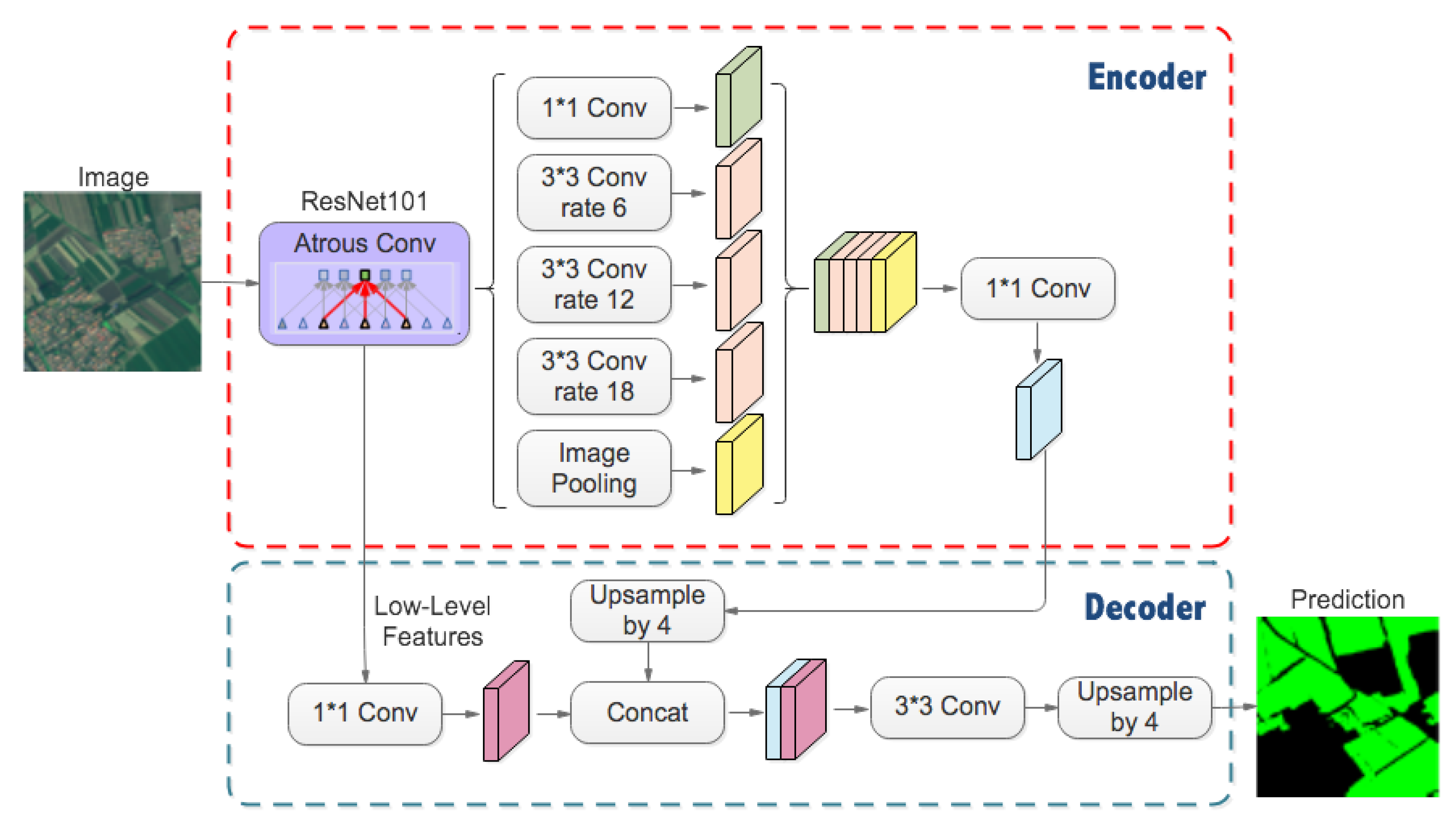
In the last few years, semantic segmentation has been a hot topic in computer vision. A number of network architectures have been proposed, e.g., FCN [58], U-Net [59], PspNet [60], SegNet [61], and DeepLab series [62,63,64,65]. Meanwhile, there have been some studies focusing on semantic segmentation for RS images. From the first attempt by Mnih and Hinton [66], who designed a shallow, fully connected network for road classification, different CNN architectures have been proposed for remote sensing images [67,68]. Recently, semantic segmentation networks that are popular in computer vision have been introduced to the field of RS image classification, and the results indicate that the networks are appropriate for RS images as well. In this study, we chose the DeepLabv3+ architecture (Figure 3), which has achieved state-of-the-art performance on the PASCAL VOC 2012 [69] and Cityscapes [70] datasets.
DeepLabv3+ is built on a powerful CNN backbone architecture for the most accurate results. It is an encoder–decoder architecture that employs DeepLabv3 to encode the rich contextual information and a simple yet effective decoder module to recover object boundaries. Moreover, the spatial pyramid pooling strategy is applied in the network structure, resulting in a faster and stronger encoder–decoder network for semantic segmentation. Although the DeepLabv3+ model was designed for natural image segmentation, it is compatible with multichannel inputs and is sensitive to the boundaries in the images. So, DeepLabv3+ is particularly suitable for RS images classification and CA boundary delineation.
3.2. Network Training and Classification
Compared with traditional computer vision images, such as the images on ImageNet, RS images often have more coverage and a larger size. So, it is difficult to train RS images as a whole. Therefore, before training, we split the labeled RS images into small parts. As RS images labeled with the GT are limited, we used a sliding window for overlapped sampling rather than the general sampling procedure. The sliding window can help expand the training dataset and avoid overfitting. Meanwhile, four forms of data augmentation (rotate 90°, rotate 180°, rotate 270°, and flip) were also used in this work to further enlarge the dataset. The expanded training dataset, which is organized by Image–GT label pairs, was then inputted into DeepLabv3+ as the source of training samples. For better and faster training results, the model was first trained on ImageNet and then transferred to our dataset. The Softmax function [71] was performed on the output feature map generated by the network to predict the class distribution. Then, the softmax loss was calculated and back-propagated, and finally, the network parameters were updated using Stochastic Gradient Descent (SGD) with momentum.
In the mapping stage, the trained network was used on the RS images to be classified. However, high spatial resolution RS images are often too large to be processed in only one pass through a CNN. Given current Graphic Processing Unit (GPU) memory limitations, we split our images into small patches using the same image size as that used in the training dataset. When splitting, an overlap strategy was also used. After predicting, we combined all of these small patches in order. For the overlapped part of the image predicted, we averaged the multiple predictions to obtain the final classification for overlapping pixels. This smooths the predictions along the borders of each patch and removes potential discontinuities.
3.3. Evaluation Method
3.3.1. Accuracy Evaluation Indicators
We employed the overall accuracy (OA), F1-Score, and Kappa coefficient as indicators to evaluate our approach. These indexes are calculated from the confusion matrix, where the overall accuracy is calculated as
where represent the total number of correctly classified pixels, and n is the total number of validation pixels. Overall accuracy denotes the proportion of the pixels that are correctly classified, and the F1-Score is computed as
where the number of true positives for class i; the number of pixels belonging to class i; and the number of pixels attributed to class i by the model. So, is the number of correct positive results divided by the number of all positive results returned by the classifier, is the number of correct positive results divided by the number of all relevant samples, and F1-Score represents the harmonic average of the and . The Kappa coefficient measures the consistency of the predicted classes with the GT classes, which is calculated as
where is the number of times rater k predicted category i. The equations show that OA is the relative observed agreement among raters, and is the hypothetical probability of chance agreement. If the raters are in complete agreement, then . If there is no agreement among the raters other than what would be expected by chance (as given by ), .
3.3.2. Per-Pixel Accuracy Evaluation Method
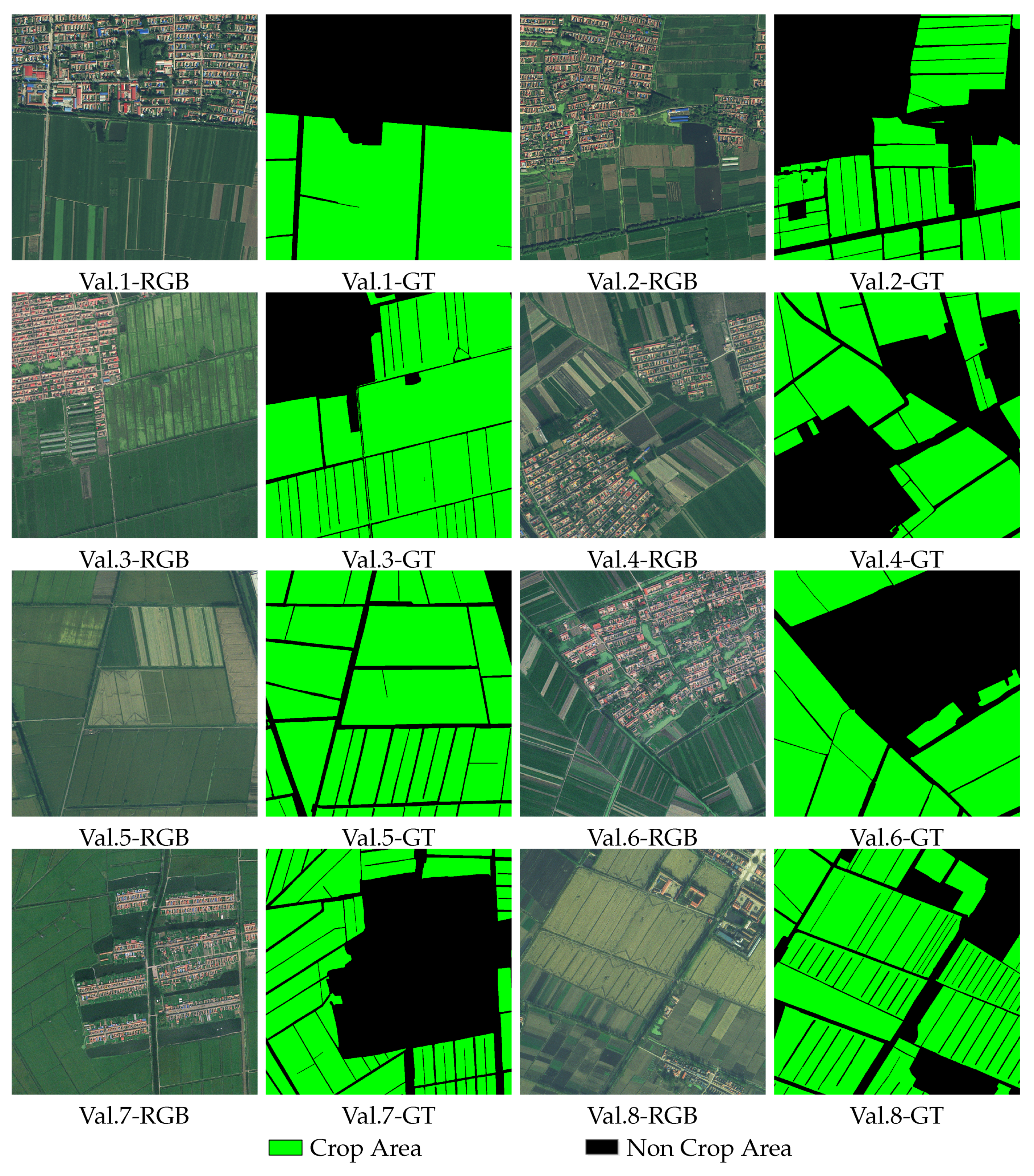
We randomly chose eight slices of the whole image for the pixel-based classification evaluation (Figure 4). The size is 1024 × 1024 for all eight, and they were all labeled manually with the GT. None of the eight slices were involved in training. By obtaining the final mapping result and calculating the confusion matrix, we obtained the OA, kappa coefficient, and F1-Score for each slice. Furthermore, per-pixel accuracy was calculated for acquiring information on the spatial distribution of the classification error. Different kinds of competing methods were processed to prove the superiority of the method proposed in this paper.
3.3.3. Random Validation Point Accuracy Evaluation Method
As the RS images we used in this study have a high spatial resolution and cover the whole Baodi county at almost 1500 km2, it is hard to do per-pixel accuracy evaluation all across the study area. So, the evaluation was carried out using validation points to further prove that the classification method is effective for the whole study area. One hundred validation points were collected randomly from the entire image and labeled by visual interpretation. With the classification results, the confusion matrix was also calculated, along with the OA, kappa coefficient, and F1-Score.
4. Experiments and Comparison
4.1. Experiment Setup
Our training dataset a collection from WV-2 of Baodi, Tianjin, China. The images are in true color fusion with a 1-meter resolution. As the training dataset structure has a great influence on training and the classification result, we used K-MEANS, an unsupervised clustering method, before sampling to ensure that different kinds of CAs in the study area are covered in the training samples. After clustering, we manually labeled eight slices (sizes of 2048 × 2048) of the whole image at the pixel level as GT label data. In our training dataset, using a sliding window with a stride of 32 pixels, there are a total of 120,000 pairs of samples (sizes of 128 × 128). So, each pixel in the RS images corresponds to a pixel class. We used 96,000 images (80% of the whole set) for training, and the remaining 24,000 images (20% of the whole set) were used for testing. We used ResNet-101 as the network backbone in the DeepLabv3+ model. The ResNet-101 model was pretrained on ImageNet and then adapted to our dataset with 0.00001 as the initial learning rate. The max iteration in our training step was 75,000. In the training procedure, we fed the samples into the network in batches, and each batch contained 16 images. For the classification stage, we split the whole predicted image into small patches with a sliding window whose stride was 32 pixels. Then, all the patches were combined, and an averaging method was applied for the overlapped parts. In addition, we used the deep learning framework TensorFlow, Compute Unified Device Architecture 8.0 (CUDA 8.0), and Geospatial Data Abstraction Library (GDAL) to construct a platform for all of the work steps, including sampling, training, testing, and classifying, to extract and map CA.
4.2. Competing Method
Traditional machine learning methods have been widely used in the field of RS classification in the last few years. Common methods include Maximum Likelihood (ML) [72], Support Vector Machine (SVM) [73], and Random Forest (RF) [74]. To prove that CNNs can get more thorough spatial or shape features from RGB high spatial resolution RS images, all three of these common classification methods were implemented using the same training dataset that we mentioned before. Detailed parameters are shown in Table 1.
Different kinds of CNNs have been used recently for RS image classification for their ability to learn both spatial and spectral information. In this paper, to show the superiority of DeepLabv3+ for the task of CA mapping, we chose four popular end-to-end structure networks, i.e., U-Net, PspNet, SegNet, and DeepLabv2, as competing networks. The training strategy and parameters were the same for all five networks. Similar to the above, the training dataset was the same here, as well.
5. Results
In this section, we compare our proposed method with other existing methods, including not only other CNNs but also traditional machine learning methods. These results represent an exhaustive and complete validation of our method with other popular methods for high spatial resolution RS image classification, and they show CNNs’ ability to learn more thorough spatial features from high spatial resolution RS images compared with other methods.
5.1. Results across DeepLabv3+
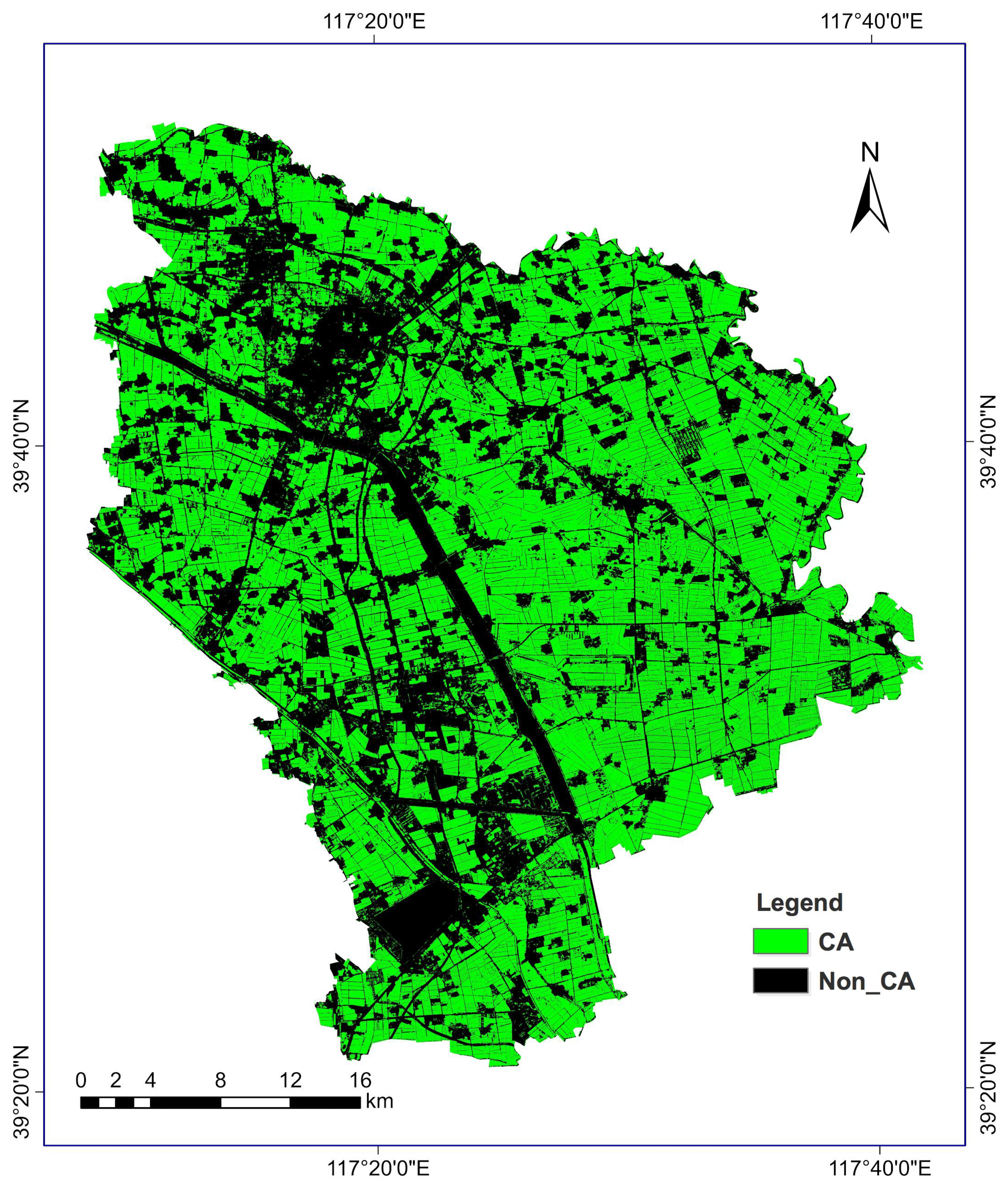
CA classification efforts in previous studies using different spatial resolution RS images have indicated that it is important to take full advantage of context and shape features in the mapping process, especially for smallholder agriculture. This inspired us to use deep semantic segmentation networks to get not only a more thorough spatial understanding but also more accurate CA mapping results automatically from RGB-only WV-2 images in this study. The image size was 49,895 × 56,044, the classification step length was 32 pixels, and the processing time was about 346 min. The processing burden rises with the increase in image size and the decrease in step length. The mapping result and confusion matrix for DeepLabv3+ for the whole image of Baodi are shown in Figure 5 and Table 2, respectively.
As can be seen, as a result of DeepLabv3+’s ability to learn context and shape features, along with its effectiveness in defining boundaries, the proposed method achieved high accuracy in the study area on the basis of RGB-only high spatial resolution remote sensing images. Linear objects, such as narrow roads and ridges between field blocks, were extracted from the CA mapping results. Furthermore, it is worth noticing that CAs with different crop types were extracted at the same time. This may result from the training dataset organization and deep semantic segmentation networks’ advantages of understanding spatial features.
To further justify the performance of the proposed methodology, four other deep semantic segmentation networks and three traditional machine learning methods were tested on eight valid slices of about 1 km2 of Baodi county. Then, a per-pixel accuracy evaluation was processed, as shown in the next two sections. The mapping results of these competing methods for the entirety of Baodi county are not shown in this paper because the main focus is on the method itself and its comparison with other methods, such as SegNet and RF.
5.2. Comparison with Other Semantic Segmentation Networks
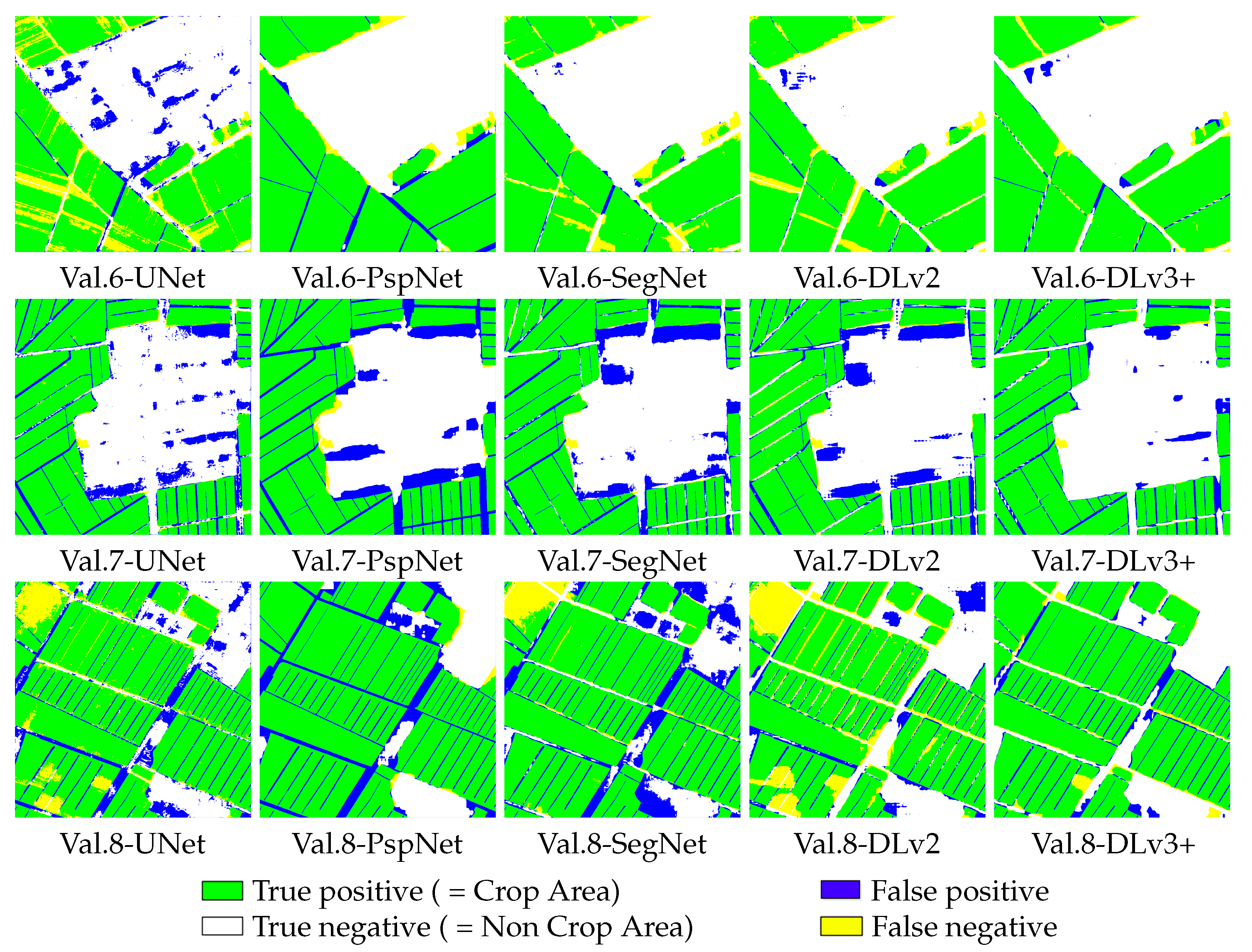
The previous result demonstrates that DeepLabv3+ can achieve high accuracy for CA classification. We tested four other deep learning methods, including SegNet, U-net, PspNet, and DeepLabv2, as described in this section. The OA, kappa coefficient, and F1-Score of each method for different categories are shown in Table 3 and Table 4, along with those of DeepLabv3+. The tables show that DeepLabv3+ obtains the best performance compared with the others, and it is apparent that DeepLab series can get better CA mapping results. SegNet has a good balance between accuracy and computational cost. Although it has a simpler architecture compared with the others, SegNet still presents a similar accuracy to that of U-Net and PspNet.
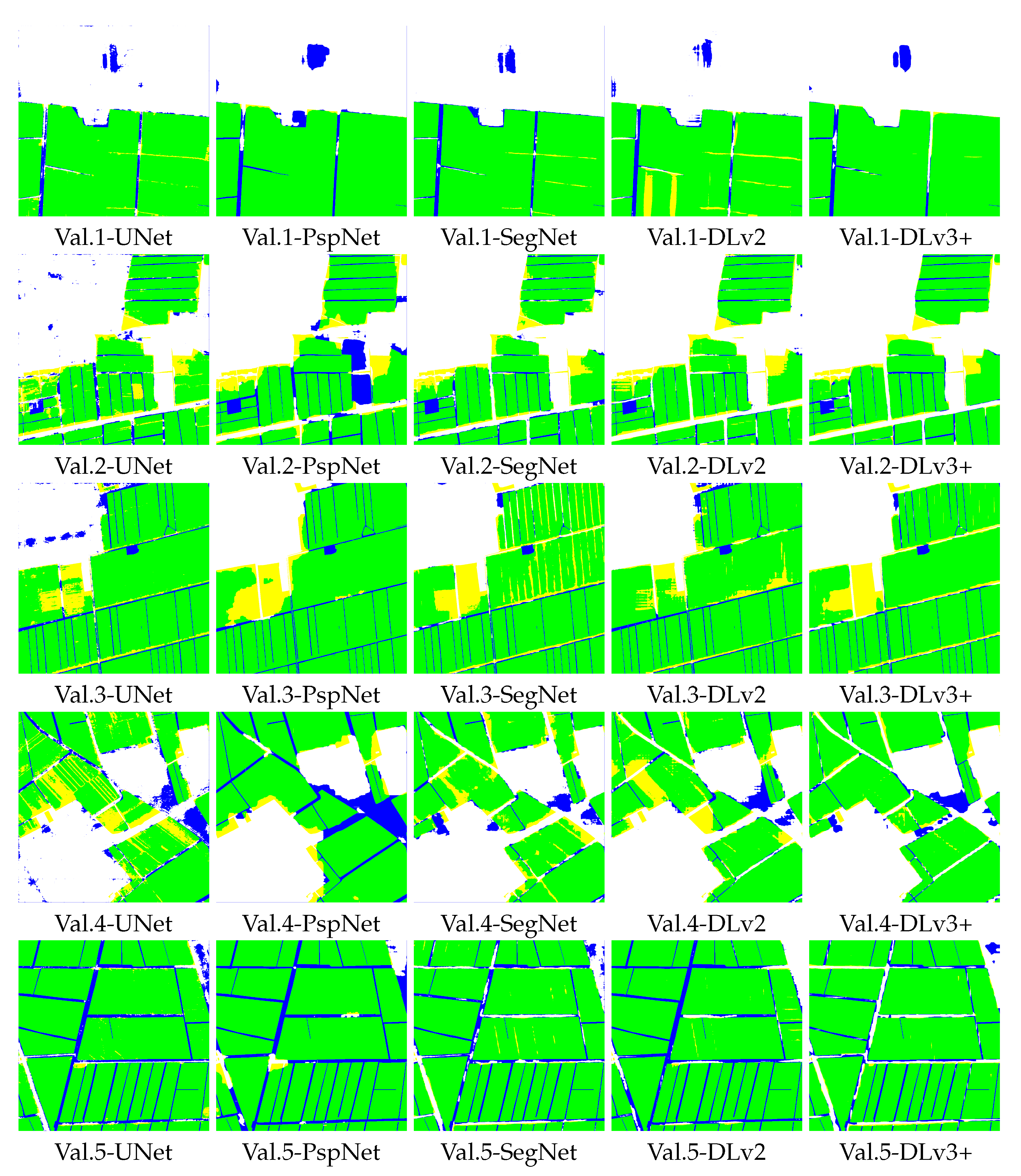
Figure 6 shows the per-pixel accuracy for all five networks on eight validation slices. The first observation is that the classification maps from the five networks are similar to each other in some way. The deep semantic networks all perform well in the prediction of CA with different kinds of crops, and they are good at region extraction from original remote sensing images. Some small and scattered objects, such as country roads and brushland with small areas, are classified correctly. On the other hand, some pixels in grassland and brushland are assigned to CA. Larger area trees, shrubland, grassland, and cropland have similar spectral properties and topographic information, so it is difficult for the trained networks to distinguish between them. Meanwhile, the trained networks receive a low accuracy when it comes to mulch, which can be seen in Val.3. This may result from the lack of training samples of this type, so the networks did not learn the corresponding features in the training stage. However, there are still some differences between the classification maps from the five networks. The DeepLab series is better at classification for the pixels that are on the edge of the image. DeepLabv3+ describes the shape and the edge of the cropland more precisely and performs better on the brushes and trees located between buildings.
5.3. Comparison between CNNs and Traditional Machine Learning Methods
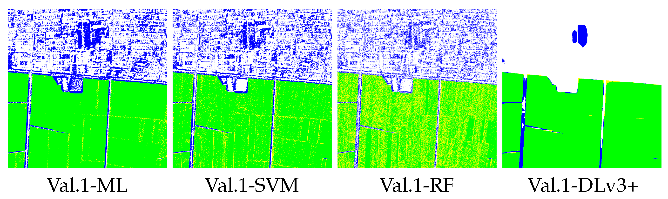
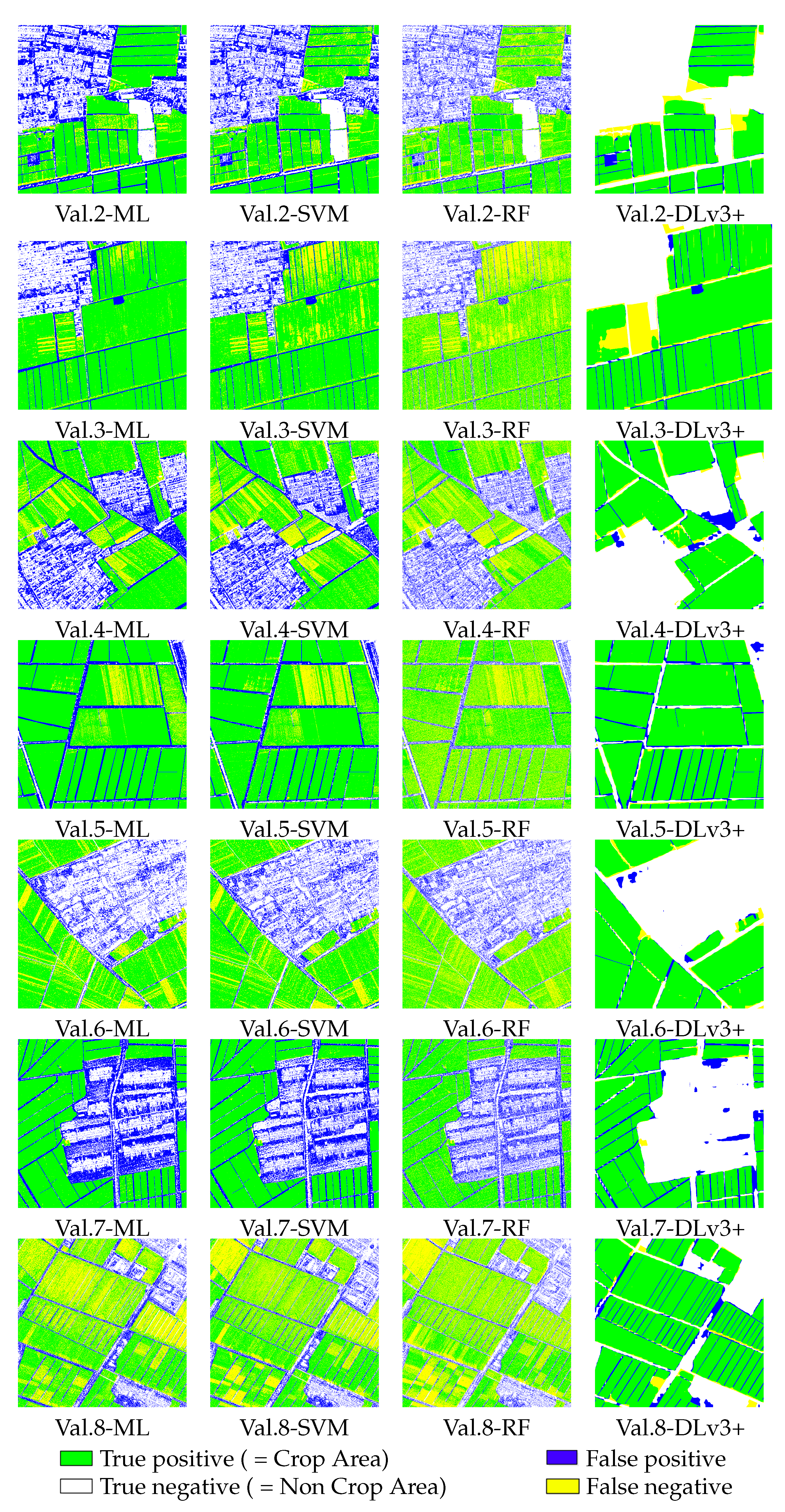
To verify the effectiveness of CNNs, we calculated the average accuracy of the five deep semantic segmentation networks and compared it with that of three traditional machine learning methods, i.e., ML, SVM, and RF. Table 5 shows accuracy evaluation results from all three models and the average results from CNNs. The three traditional machine learning methods perform similarly to each other and have an average OA of 70.27%, while CNNs show a significant increase in OA (19.18%). The F1-Score shown in Table 6 also indicates that CNNs have a higher accuracy in the classification of CA. Traditional machine learning methods create a serious salt-and-pepper phenomenon in the classification maps, which can be seen in Figure 7. Using object-based classification may solve this problem, but object segmentation is a highly subjective process that needs researchers to set up the segmentation parameters on the basis of experience. However, the deep semantic segmentation networks we used can perform the segmentation automatically and classify pixels at the same time. The results prove that the deep semantic segmentation networks are effective in both segmentation and classification.
6. Discussion
Mapping CA using remotely sensed observations is important for CA protection and agricultural production. However, existing CA maps are mostly based on medium or low spatial resolution RS images that lack the essential spatial details to describe CA in a smallholder family farming system. Taking advantage of high spatial resolution RS images is an effective way to solve this problem, but it still presents several challenges when the traditional machine learning methods are used. These challenges include a thorough understanding of the rich spatial features and classification with low spectral resolution. Faced with these challenges, we developed an automatic classification framework based on deep semantic segmentation networks to map CA from WV-2 images with only three bands of RGB. Our study area, Baodi, has various types of soil and crops. It is an important grain and cotton production base in northern China. The climate and topographic conditions in the area are common in the North China Plain. All of these aspects make it representative for use in this study. Our research provides a number of key insights into how to utilize high spatial resolution RS images and deep semantic segmentation networks for mapping CA in a smallholder agricultural system.
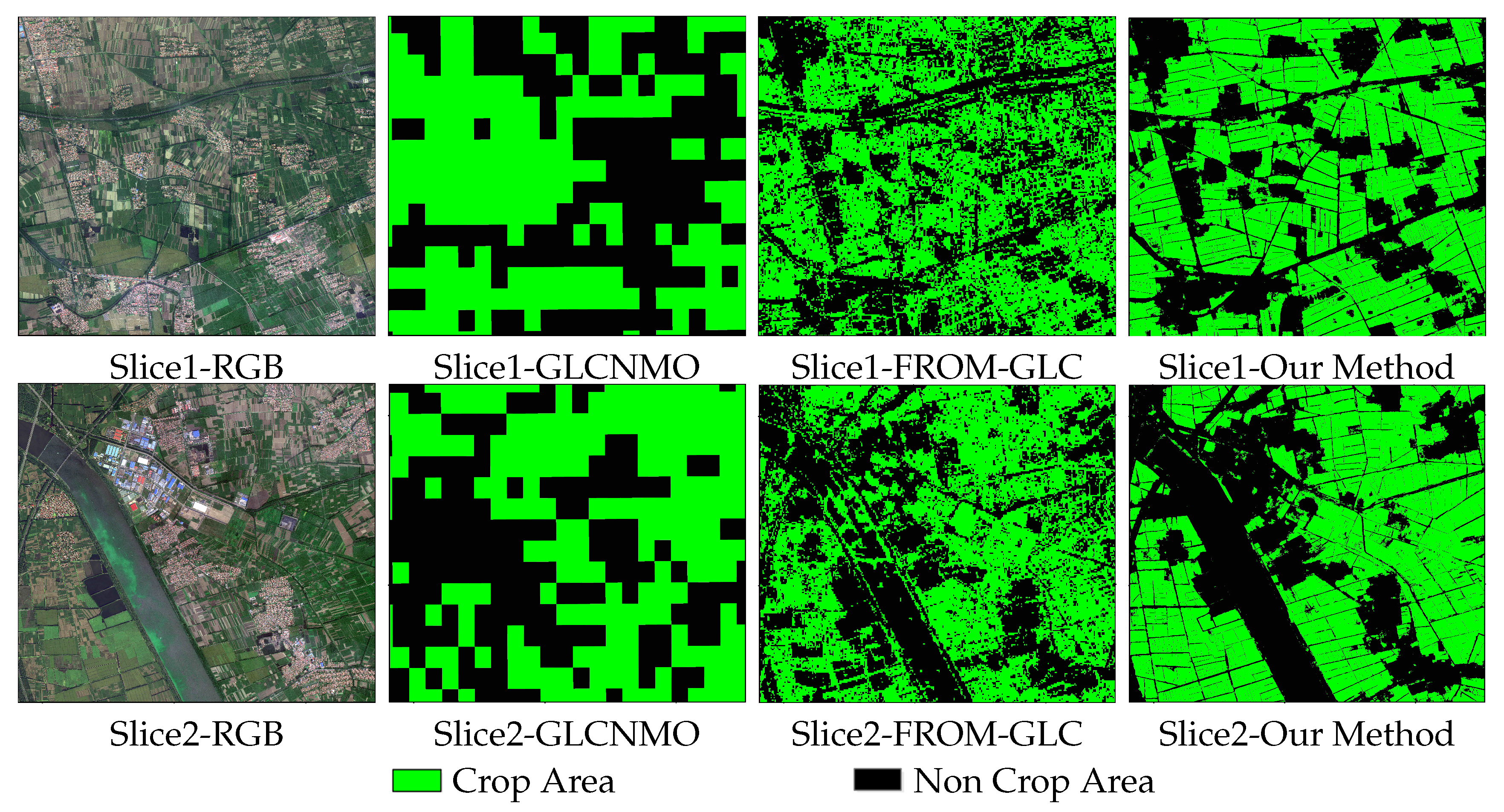
First, our study demonstrates that, on the basis of high spatial resolution RS images and deep semantic segmentation networks, our method is suitable for the classification of CA in a smallholder family farming system. We compared our CA map with some other existing maps of Baodi. The Global Map–Global LC (GLCNMO) dataset from the International Steering Committee for Global Mapping, 2008, 500 m resolution [11] and the Finer Resolution Observation and Monitoring Global LC dataset (FROM-GLC) from China based on Landsat images, 2015, 30 m resolution [16] were used here. The same validation sample points introduced in Section 3.3.3 were utilized to prove the effectiveness of high spatial resolution RS images and the method proposed in this study. Table 7 shows the OA and kappa coefficient of the GLCNMO and FROM-GLC datasets and our result. The FROM-GLC dataset performs better than the GLCNMO dataset in the accuracy evaluation result, but they are very similar to each other. Results from our method show a significant increase in the OA and kappa coefficient. A comparison of the detailed mapping results is shown in Figure 8. The sharpness of the CA boundaries and the details in the classification results are increased with the spatial resolution of RS images. The shape and contour of the road and river are also clearer in the results of WV-2 images. Further, the method proposed in this paper is better with the brushes and trees located between buildings and gives a more precise location of the CA in the mapping results, which is important for the small-sized fields in the smallholder family farming system.
A second major insight from our study is that deep semantic segmentation networks are effective in feature extraction from high spatial resolution RS images. Traditional machine learning methods usually rely on hand-engineered features to describe the spectral, contextual, and shape features of the input images. Most appearance descriptors depend on a set of free parameters, which are commonly set by user experience via experimental trial-and-error or cross-validation. However, as a sort of CNN, deep semantic segmentation networks are able to automatically discover relevant features in classification problems. Furthermore, the network used in this study, DeepLabv3+, can capture multi-scale information and generalize the standard convolution operation by the atrous convolution, which results in a more thorough understanding of the input information.
A third major insight is that deep semantic segmentation networks can prevent the salt-and-pepper phenomenon, which is common in pixel-based high spatial resolution RS image classification tasks. Before the appearance of deep semantic segmentation networks, the object-based classification method was usually used to solve the salt-and-pepper problem [75,76], but object segmentation also relies on researchers’ experience and knowledge to set up the segmentation parameters. However, a deep semantic segmentation network can perform segmentation and pixel classification at the same time by its encoder–decoder structure and obtain high classification accuracy and more detailed boundaries of CA. Therefore, compared with traditional machine learning methods, deep semantic segmentation can get better CA classification results, especially when it comes to high spatial resolution RS images with low spectral resolution.
A final key insight from our study is that it is possible to apply deep learning methods to the larger-scale task of RS image classification. Deep learning techniques were originally rooted in the computer vision fields for classification and recognition tasks, and they have only recently been introduced to the RS community. As a new research branch in RS image analysis, most of the recent studies have focused on the optimization of models and algorithms using a small-scale study area [77,78]. Studies using deep learning models for larger-scale RS classification are lacking. However, classification over large areas is one of the fundamental topics in the RS application field. In this study, we applied the proposed method to classify the CA of Baodi, which occupies 1500 km2. With the development of hardware and the improvement of model training strategies, problems such as low efficiency and large numbers of training samples may be solved, and then deep learning models can be applied to the classification (or other analysis) of larger study areas, such as those at the regional or even national level.
Our method yielded automatic and precise smallholder agricultural CA maps, but a few uncertainties remain. First, our classification framework performed well with only one single-phase RS image and three RGB bands in this study. However, multi-temporal and multi-spectral features may help optimize the CA mapping results. Furthermore, although traditional machine learning methods had a lower classification accuracy, they were easier to train on a smaller dataset with point labels, and they had a higher efficiency in both the training and classification stages. The great performance of deep semantic segmentation models is often due to the availability of massive datasets. However, recent studies on semi-supervised [79] or even unsupervised [80] deep learning methods, as well as the transfer learning strategy [81], indicate that this problem can be solved.
7. Conclusions
Prior studies have documented the effectiveness of RS image classification for the purpose of CA protection. However, these studies have been mostly based on RS images with medium or low spatial resolution, neglecting high spatial resolution RS images’ advantages for precise smallholder agriculture observation. Meanwhile, the methods used in these studies have often lacked a more thorough understanding of the context, such as the shape of objects. In this paper, using CNNs and WV-2 images, we developed a methodology to get better shapes and deeper contextual features of cropland, and we accomplished the automatic mapping of the CA of satellite images with only the three RGB bands.
We found that deep semantic segmentation networks, as a sort of CNN, are able to automatically extract the deep features from the input images and prevent salt-and-pepper problems by their encoder–decoder structure. Therefore, methods based on deep semantic segmentation models can get a higher classification accuracy and more detailed boundaries of CA than traditional machine learning methods, such as ML, SVM, and RF. These findings indicate that the deep semantic segmentation networks are effective for both the segmentation and classification of high spatial resolution RS images. Furthermore, we used the proposed method to classify the CA of the whole study area, which occupies 1500 km2. This study, therefore, provides insight into introducing deep learning methods to the larger-scale task of RS image classification.
Most notably, to our knowledge, this is the first study to use CNNs to extract the CA of a whole county area. Our results provide compelling evidence for CNNs’ ability to learn shape and contextual features and show that this approach appears to be effective for smallholder agriculture CA mapping. Owing to the representativeness of the study area and the generalization of the proposed framework, the methodology can be applied to other similar areas in the North China Plain or extended to mapping more refined cropland attributes such as crop types. However, there are still some limitations worth noting. Although our method achieved high accuracy in the study with only one single-phase RS image and three RGB bands, multi-temporal RS images and the near-infrared band have been proved to be important for CA classification. Future work should, therefore, focus on multi-source RS image fusion and multi-time sequence data processing with recurrent neural networks (RNNs).
Author Contributions
As the first author, Z.D. proposed the main structure of this study, and contributed to experiments, data analysis and manuscript writing. J.Y. mainly contribute to manuscript revision. C.O. gave some advice on experiment designing. T.Z. contributed to WV-2 data preprocessing.
Funding
This research was funded by Special Fund for Scientific Research on Public Causes grant number 201511010-06.
Acknowledgments
The authors would like to thank Quanlong Feng, Quanquan Xu for their suggestions in improving both the structure and the details of this paper. Particular thanks to Prof. Atzberger and the three anonymous referees for very useful comments and suggestions.
Conflicts of Interest
The authors declare no conflict of interest. The funders had no role in the design of the study; in the collection, analyses, or interpretation of data; in the writing of the manuscript, or in the decision to publish the results.
References
- Cui, K.; Shoemaker, S.P. A look at food security in China. Sci. Food 2018, 2, 4. [Google Scholar] [CrossRef]
- Huang, J.; Ma, H.; Sedano, F.; Lewis, P.; Liang, S.; Wu, Q.; Su, W.; Zhang, X.; Zhu, D. Evaluation of regional estimates of winter wheat yield by assimilating three remotely sensed reflectance datasets into the coupled WOFOST–PROSAIL model. Eur. J. Agron. 2019, 102, 1–13. [Google Scholar] [CrossRef]
- Huang, J.; Sedano, F.; Huang, Y.; Ma, H.; Li, X.; Liang, S.; Tian, L.; Zhang, X.; Fan, J.; Wu, W. Assimilating a synthetic Kalman filter leaf area index series into the WOFOST model to improve regional winter wheat yield estimation. Agric. For. Meteorol. 2016, 216, 188–202. [Google Scholar] [CrossRef]
- Huang, J.; Tian, L.; Liang, S.; Ma, H.; Becker-Reshef, I.; Huang, Y.; Su, W.; Zhang, X.; Zhu, D.; Wu, W. Improving winter wheat yield estimation by assimilation of the leaf area index from Landsat TM and MODIS data into the WOFOST model. Agric. For. Meteorol. 2015, 204, 106–121. [Google Scholar] [CrossRef]
- Huang, J.; Ma, H.; Su, W.; Zhang, X.; Huang, Y.; Fan, J.; Wu, W. Jointly assimilating MODIS LAI and ET products into the SWAP model for winter wheat yield estimation. IEEE J. Sel. Top. Appl. Earth Obs. Remote Sens. 2015, 8, 4060–4071. [Google Scholar] [CrossRef]
- Xiong, J.; Thenkabail, P.S.; Gumma, M.K.; Teluguntla, P.; Poehnelt, J.; Congalton, R.G.; Yadav, K.; Thau, D. Automated cropland mapping of continental Africa using Google Earth Engine cloud computing. ISPRS J. Photogramm. Remote Sens. 2017, 126, 225–244. [Google Scholar] [CrossRef]
- Lowder, S.K.; Skoet, J.; Raney, T. The number, size, and distribution of farms, smallholder farms, and family farms worldwide. World Dev. 2016, 87, 16–29. [Google Scholar] [CrossRef]
- Phalke, A.R.; Özdoğan, M. Large area cropland extent mapping with Landsat data and a generalized classifier. Remote Sens. Environ. 2018, 219, 180–195. [Google Scholar] [CrossRef]
- Loveland, T.R.; Reed, B.C.; Brown, J.F.; Ohlen, D.O.; Zhu, Z.; Yang, L.; Merchant, J.W. Development of a global land cover characteristics database and IGBP DISCover from 1 km AVHRR data. Int. J. Remote Sens. 2000, 21, 1303–1330. [Google Scholar] [CrossRef]
- Friedl, M.A.; Sulla-Menashe, D.; Tan, B.; Schneider, A.; Ramankutty, N.; Sibley, A.; Huang, X. MODIS Collection 5 global land cover: Algorithm refinements and characterization of new datasets. Remote Sens. Environ. 2010, 114, 168–182. [Google Scholar] [CrossRef]
- Tateishi, R.; Hoan, N.T.; Kobayashi, T.; Alsaaideh, B.; Tana, G.; Phong, D.X. Production of global land cover data–GLCNMO2008. J. Geogr. Geol. 2014, 6, 99. [Google Scholar] [CrossRef]
- Chen, B.; Huang, B.; Xu, B. Multi-source remotely sensed data fusion for improving land cover classification. ISPRS J. Photogramm. Remote Sens. 2017, 124, 27–39. [Google Scholar] [CrossRef]
- Azzari, G.; Lobell, D. Landsat-based classification in the cloud: An opportunity for a paradigm shift in land cover monitoring. Remote Sens. Environ. 2017, 202, 64–74. [Google Scholar] [CrossRef]
- Kirches, G.; Brockmann, C.; Boettcher, M.; Peters, M.; Bontemps, S.; Lamarche, C.; Schlerf, M.; Santoro, M.; Defourny, P. Land Cover CCI Product User Guide: Version 2; ESA Public Document CCI-LC-PUG; European Space Agency: Paris, France, 2014; p. 4. [Google Scholar]
- Chen, J.; Chen, J.; Liao, A.; Cao, X.; Chen, L.; Chen, X.; He, C.; Han, G.; Peng, S.; Lu, M.; et al. Global land cover mapping at 30 m resolution: A POK-based operational approach. ISPRS J. Photogramm. Remote Sens. 2015, 103, 7–27. [Google Scholar] [CrossRef]
- Yu, L.; Wang, J.; Gong, P. Improving 30 m global land-cover map FROM-GLC with time series MODIS and auxiliary data sets: A segmentation-based approach. Int. J. Remote Sens. 2013, 34, 5851–5867. [Google Scholar] [CrossRef]
- Belgiu, M.; Csillik, O. Sentinel-2 cropland mapping using pixel-based and object-based time-weighted dynamic time warping analysis. Remote Sens. Environ. 2018, 204, 509–523. [Google Scholar] [CrossRef]
- Griffiths, P.; Nendel, C.; Hostert, P. Intra-annual reflectance composites from Sentinel-2 and Landsat for national-scale crop and land cover mapping. Remote Sens. Environ. 2019, 220, 135–151. [Google Scholar] [CrossRef]
- Immitzer, M.; Vuolo, F.; Atzberger, C. First experience with Sentinel-2 data for crop and tree species classifications in central Europe. Remote Sens. 2016, 8, 166. [Google Scholar] [CrossRef]
- Vuolo, F.; Neuwirth, M.; Immitzer, M.; Atzberger, C.; Ng, W.T. How much does multi-temporal Sentinel-2 data improve crop type classification? Int. J. Appl. Earth Obs. Geoinf. 2018, 72, 122–130. [Google Scholar] [CrossRef]
- Castillo, J.A.A.; Apan, A.A.; Maraseni, T.N.; Salmo III, S.G. Estimation and mapping of above-ground biomass of mangrove forests and their replacement land uses in the Philippines using Sentinel imagery. ISPRS J. Photogramm. Remote Sens. 2017, 134, 70–85. [Google Scholar] [CrossRef]
- Clevers, J.; Kooistra, L.; Van Den Brande, M. Using Sentinel-2 data for retrieving LAI and leaf and canopy chlorophyll content of a potato crop. Remote Sens. 2017, 9, 405. [Google Scholar] [CrossRef]
- Zhang, X.; Du, S. Learning selfhood scales for urban land cover mapping with very-high-resolution satellite images. Remote Sens. Environ. 2016, 178, 172–190. [Google Scholar] [CrossRef]
- Feng, Q.; Liu, J.; Gong, J. UAV remote sensing for urban vegetation mapping using random forest and texture analysis. Remote Sens. 2015, 7, 1074–1094. [Google Scholar] [CrossRef]
- Neigh, C.S.; Carroll, M.L.; Wooten, M.R.; McCarty, J.L.; Powell, B.F.; Husak, G.J.; Enenkel, M.; Hain, C.R. Smallholder crop area mapped with wall-to-wall WorldView sub-meter panchromatic image texture: A test case for Tigray, Ethiopia. Remote Sens. Environ. 2018, 212, 8–20. [Google Scholar] [CrossRef]
- See, L.; McCallum, I.; Fritz, S.; Perger, C.; Kraxner, F.; Obersteiner, M.; Deka Baruah, U.; Mili, N.; Ram Kalita, N. Mapping cropland in Ethiopia using crowdsourcing. Int. J. Geosci. 2013, 4, 6–13. [Google Scholar] [CrossRef]
- Yang, C.; Everitt, J.H.; Murden, D. Evaluating high resolution SPOT 5 satellite imagery for crop identification. Comput. Electron. Agric. 2011, 75, 347–354. [Google Scholar] [CrossRef]
- Tseng, M.H.; Chen, S.J.; Hwang, G.H.; Shen, M.Y. A genetic algorithm rule-based approach for land-cover classification. ISPRS J. Photogramm. Remote Sens. 2008, 63, 202–212. [Google Scholar] [CrossRef]
- Khatami, R.; Mountrakis, G.; Stehman, S.V. A meta-analysis of remote sensing research on supervised pixel-based land-cover image classification processes: General guidelines for practitioners and future research. Remote Sens. Environ. 2016, 177, 89–100. [Google Scholar] [CrossRef]
- Clausi, D.A. An analysis of co-occurrence texture statistics as a function of grey level quantization. Can. J. Remote Sens. 2002, 28, 45–62. [Google Scholar] [CrossRef]
- Barber, D.G.; Ledrew, E.F. SAR Sea Ice Discrimination Using Texture Statistics: A Multivariate Approach. Photogramm. Eng. Remote Sens. 1991, 57, 385–395. [Google Scholar]
- Pesaresi, M.; Benediktsson, J.A. A new approach for the morphological segmentation of high-resolution satellite imagery. IEEE Trans. Geosci. Remote Sens. 2001, 39, 309–320. [Google Scholar] [CrossRef]
- Chen, T.; Trinder, J.C.; Niu, R. Object-oriented landslide mapping using ZY-3 satellite imagery, random forest and mathematical morphology, for the Three-Gorges Reservoir, China. Remote Sens. 2017, 9, 333. [Google Scholar] [CrossRef]
- Zhang, W.; Sun, X.; Fu, K.; Wang, C.; Wang, H. Object detection in high-resolution remote sensing images using rotation invariant parts based model. IEEE Geosci. Remote Sens. Lett. 2014, 11, 74–78. [Google Scholar] [CrossRef]
- Cheng, G.; Zhou, P.; Han, J. Learning rotation-invariant convolutional neural networks for object detection in VHR optical remote sensing images. IEEE Trans. Geosci. Remote Sens. 2016, 54, 7405–7415. [Google Scholar] [CrossRef]
- LeCun, Y.; Bottou, L.; Bengio, Y.; Haffner, P. Gradient-based learning applied to document recognition. Proc. IEEE 1998, 86, 2278–2324. [Google Scholar] [CrossRef]
- Ding, P.; Zhang, Y.; Deng, W.J.; Jia, P.; Kuijper, A. A light and faster regional convolutional neural network for object detection in optical remote sensing images. ISPRS J. Photogramm. Remote Sens. 2018, 141, 208–218. [Google Scholar] [CrossRef]
- Kellenberger, B.; Marcos, D.; Tuia, D. Detecting mammals in UAV images: Best practices to address a substantially imbalanced dataset with deep learning. Remote Sens. Environ. 2018, 216, 139–153. [Google Scholar] [CrossRef]
- Zhang, F.; Du, B.; Zhang, L. Scene classification via a gradient boosting random convolutional network framework. IEEE Trans. Geosci. Remote Sens. 2016, 54, 1793–1802. [Google Scholar] [CrossRef]
- Liu, Q.; Hang, R.; Song, H.; Li, Z. Learning multiscale deep features for high-resolution satellite image scene classification. IEEE Trans. Geosci. Remote Sens. 2018, 56, 117–126. [Google Scholar] [CrossRef]
- Huang, W.; Xiao, L.; Wei, Z.; Liu, H.; Tang, S. A new pan-sharpening method with deep neural networks. IEEE Geosci. Remote Sens. Lett. 2015, 12, 1037–1041. [Google Scholar] [CrossRef]
- Wang, S.; Quan, D.; Liang, X.; Ning, M.; Guo, Y.; Jiao, L. A deep learning framework for remote sensing image registration. ISPRS J. Photogramm. Remote Sens. 2018, 145, 148–164. [Google Scholar] [CrossRef]
- Romero, A.; Gatta, C.; Camps-Valls, G. Unsupervised deep feature extraction for remote sensing image classification. IEEE Trans. Geosci. Remote Sens. 2016, 54, 1349–1362. [Google Scholar] [CrossRef]
- Paisitkriangkrai, S.; Sherrah, J.; Janney, P.; Hengel, V.D. Effective semantic pixel labelling with convolutional networks and conditional random fields. In Proceedings of the IEEE Conference on Computer Vision and Pattern Recognition Workshops, Boston, MA, USA, 7–12 June 2015; pp. 36–43. [Google Scholar]
- Längkvist, M.; Kiselev, A.; Alirezaie, M.; Loutfi, A. Classification and segmentation of satellite orthoimagery using convolutional neural networks. Remote Sens. 2016, 8, 329. [Google Scholar] [CrossRef]
- Volpi, M.; Tuia, D. Deep multi-task learning for a geographically-regularized semantic segmentation of aerial images. ISPRS J. Photogramm. Remote Sens. 2018, 144, 48–60. [Google Scholar] [CrossRef]
- Audebert, N.; Le Saux, B.; Lefèvre, S. Beyond RGB: Very high resolution urban remote sensing with multimodal deep networks. ISPRS J. Photogramm. Remote Sens. 2018, 140, 20–32. [Google Scholar] [CrossRef]
- Liu, S.; Ding, W.; Liu, C.; Liu, Y.; Wang, Y.; Li, H. ERN: Edge Loss Reinforced Semantic Segmentation Network for Remote Sensing Images. Remote Sens. 2018, 10, 1339. [Google Scholar] [CrossRef]
- Xu, Y.; Wu, L.; Xie, Z.; Chen, Z. Building Extraction in Very High Resolution Remote Sensing Imagery Using Deep Learning and Guided Filters. Remote Sens. 2018, 10, 144. [Google Scholar] [CrossRef]
- Kemker, R.; Salvaggio, C.; Kanan, C. Algorithms for semantic segmentation of multispectral remote sensing imagery using deep learning. ISPRS J. Photogramm. Remote Sens. 2018, 145, 60–77. [Google Scholar] [CrossRef]
- Fu, G.; Liu, C.; Zhou, R.; Sun, T.; Zhang, Q. Classification for high resolution remote sensing imagery using a fully convolutional network. Remote Sens. 2017, 9, 498. [Google Scholar] [CrossRef]
- Volpi, M.; Tuia, D. Dense semantic labeling of subdecimeter resolution images with convolutional neural networks. IEEE Trans. Geosci. Remote Sens. 2017, 55, 881–893. [Google Scholar] [CrossRef]
- Sherrah, J. Fully convolutional networks for dense semantic labelling of high-resolution aerial imagery. arXiv, 2016; arXiv:1606.02585. [Google Scholar]
- Maggiori, E.; Tarabalka, Y.; Charpiat, G.; Alliez, P. Convolutional neural networks for large-scale remote-sensing image classification. IEEE Trans. Geosci. Remote Sens. 2017, 55, 645–657. [Google Scholar] [CrossRef]
- Zhang, X.; Wu, B.; Zhu, L.; Tian, F.; Zhang, M. Land use mapping in the Three Gorges Reservoir Area based on semantic segmentation deep learning method. arXiv, 2018; arXiv:1804.00498. [Google Scholar]
- Sun, J.; Zhang, H.; Li, Y. Analysis of Air Temperature and Precipitation in Baodi District and Risk Zoning for Agricultural Meteorological Disasters. Tianjin Sci. Technol. 2016, 43, 7–9. [Google Scholar]
- Shen, C.; Shen, G. Investigation and evaluation on the soil quality of cultivated land in Tianjin Baodi District. Tianjin Agric. Sci. 2013, 19, 51–55. [Google Scholar]
- Long, J.; Shelhamer, E.; Darrell, T. Fully convolutional networks for semantic segmentation. In Proceedings of the IEEE Conference on Computer Vision and Pattern Recognition, Boston, MA, USA, 7–12 June 2015; pp. 3431–3440. [Google Scholar]
- Ronneberger, O.; Fischer, P.; Brox, T. U-net: Convolutional networks for biomedical image segmentation. In Proceedings of the International Conference on Medical Image Computing and Computer-Assisted Intervention, Munich, Germany, 5–9 October 2015; pp. 234–241. [Google Scholar]
- Zhao, H.; Shi, J.; Qi, X.; Wang, X.; Jia, J. Pyramid scene parsing network. In Proceedings of the IEEE Conference on Computer Vision and Pattern Recognition (CVPR), Honolulu, HI, USA, 21–26 July 2017; pp. 2881–2890. [Google Scholar]
- Badrinarayanan, V.; Kendall, A.; Cipolla, R. Segnet: A deep convolutional encoder–decoder architecture for image segmentation. arXiv, 2015; arXiv:1511.00561. [Google Scholar]
- Chen, L.C.; Papandreou, G.; Kokkinos, I.; Murphy, K.; Yuille, A.L. Semantic image segmentation with deep convolutional nets and fully connected crfs. arXiv, 2014; arXiv:1412.7062. [Google Scholar]
- Chen, L.C.; Papandreou, G.; Kokkinos, I.; Murphy, K.; Yuille, A.L. Deeplab: Semantic image segmentation with deep convolutional nets, atrous convolution, and fully connected crfs. IEEE Trans. Pattern Anal. Mach. Intell. 2018, 40, 834–848. [Google Scholar] [CrossRef]
- Chen, L.C.; Papandreou, G.; Schroff, F.; Adam, H. Rethinking atrous convolution for semantic image segmentation. arXiv, 2017; arXiv:1706.05587. [Google Scholar]
- Chen, L.C.; Zhu, Y.; Papandreou, G.; Schroff, F.; Adam, H. Encoder–decoder with atrous separable convolution for semantic image segmentation. arXiv, 2018; arXiv:1802.02611. [Google Scholar]
- Mnih, V.; Hinton, G.E. Learning to detect roads in high-resolution aerial images. In Proceedings of the European Conference on Computer Vision, Heraklion, Crete, Greece, 5–11 September 2010; pp. 210–223. [Google Scholar]
- Marcu, A.; Leordeanu, M. Dual local-global contextual pathways for recognition in aerial imagery. arXiv, 2016; arXiv:1605.05462. [Google Scholar]
- Paoletti, M.; Haut, J.; Plaza, J.; Plaza, A. A new deep convolutional neural network for fast hyperspectral image classification. ISPRS J. Photogramm. Remote Sens. 2018, 145, 120–147. [Google Scholar] [CrossRef]
- Everingham, M.; Eslami, S.M.A.; Gool, L.V.; Williams, C.K.I.; Winn, J.; Zisserman, A. The Pascal Visual Object Classes Challenge: A Retrospective. Int. J. Comput. Vis. 2015, 111, 98–136. [Google Scholar] [CrossRef]
- Cordts, M.; Omran, M.; Ramos, S.; Rehfeld, T.; Enzweiler, M.; Benenson, R.; Franke, U.; Roth, S.; Schiele, B. The Cityscapes Dataset for Semantic Urban Scene Understanding. In Proceedings of the 2016 IEEE Conference on Computer Vision and Pattern Recognition (CVPR), Las Vegas, NV, USA, 27 June–1 July 2016. [Google Scholar]
- Krizhevsky, A.; Sutskever, I.; Hinton, G.E. ImageNet Classification with Deep Convolutional Neural Networks. In Proceedings of the International Conference on Neural Information Processing Systems, Lake Tahoe, Nevada, USA, 3–8 December 2012. [Google Scholar]
- Dempster, A.P.; Laird, N.M.; Rubin, D.B. Maximum Likelihood from Incomplete Data via the EM Algorithm. J. R. Stat. Soc. 1977, 39, 1–38. [Google Scholar] [CrossRef]
- Cortes, C.; Vapnik, V. Support-vector networks. Mach. Learn. 1995, 20, 273–297. [Google Scholar] [CrossRef]
- Cutler, A.; Cutler, D.R.; Stevens, J.R. Random Forests. Mach. Learn. 2004, 45, 157–176. [Google Scholar]
- Chen, Y.; Ge, Y.; Heuvelink, G.B.; An, R.; Chen, Y. Object-based superresolution land-cover mapping from remotely sensed imagery. IEEE Trans. Geosci. Remote Sens. 2018, 56, 328–340. [Google Scholar] [CrossRef]
- Zhang, C.; Sargent, I.; Pan, X.; Li, H.; Gardiner, A.; Hare, J.; Atkinson, P.M. An object-based convolutional neural network (OCNN) for urban land use classification. Remote Sens. Environ. 2018, 216, 57–70. [Google Scholar] [CrossRef]
- Ji, S.; Zhang, C.; Xu, A.; Shi, Y.; Duan, Y. 3D convolutional neural networks for crop classification with multi-temporal remote sensing images. Remote Sens. 2018, 10, 75. [Google Scholar] [CrossRef]
- Zhao, W.; Du, S. Learning multiscale and deep representations for classifying remotely sensed imagery. ISPRS J. Photogramm. Remote Sens. 2016, 113, 155–165. [Google Scholar] [CrossRef]
- Wu, H.; Prasad, S. Semi-supervised deep learning using pseudo labels for hyperspectral image classification. IEEE Trans. Image Process. 2018, 27, 1259–1270. [Google Scholar] [CrossRef]
- Mou, L.; Ghamisi, P.; Zhu, X.X. Unsupervised spectral–spatial feature learning via deep residual conv–deconv network for hyperspectral image classification. IEEE Trans. Geosci. Remote Sens. 2018, 56, 391–406. [Google Scholar] [CrossRef]
- Deng, C.; Xue, Y.; Liu, X.; Li, C.; Tao, D. Active Transfer Learning Network: A Unified Deep Joint Spectral-Spatial Feature Learning Model for Hyperspectral Image Classification. IEEE Trans. Geosci. Remote Sens. 2019, 57, 1741–1754. [Google Scholar] [CrossRef]
Figure 1.
Baodi county with its WorldView-2 (WV-2) images.
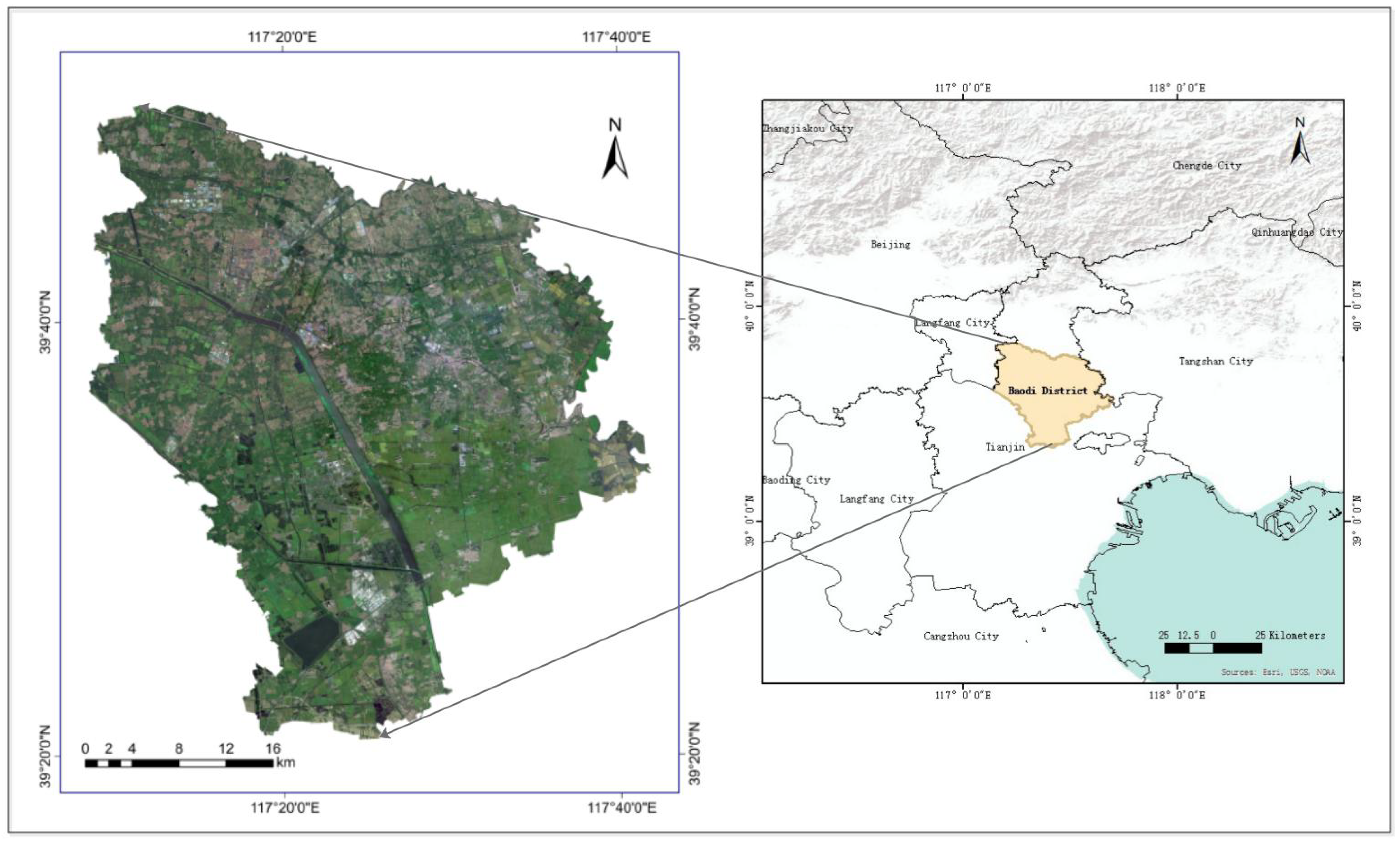
Figure 2.
Workflow for mapping crop area (CA) using DeepLabv3+.
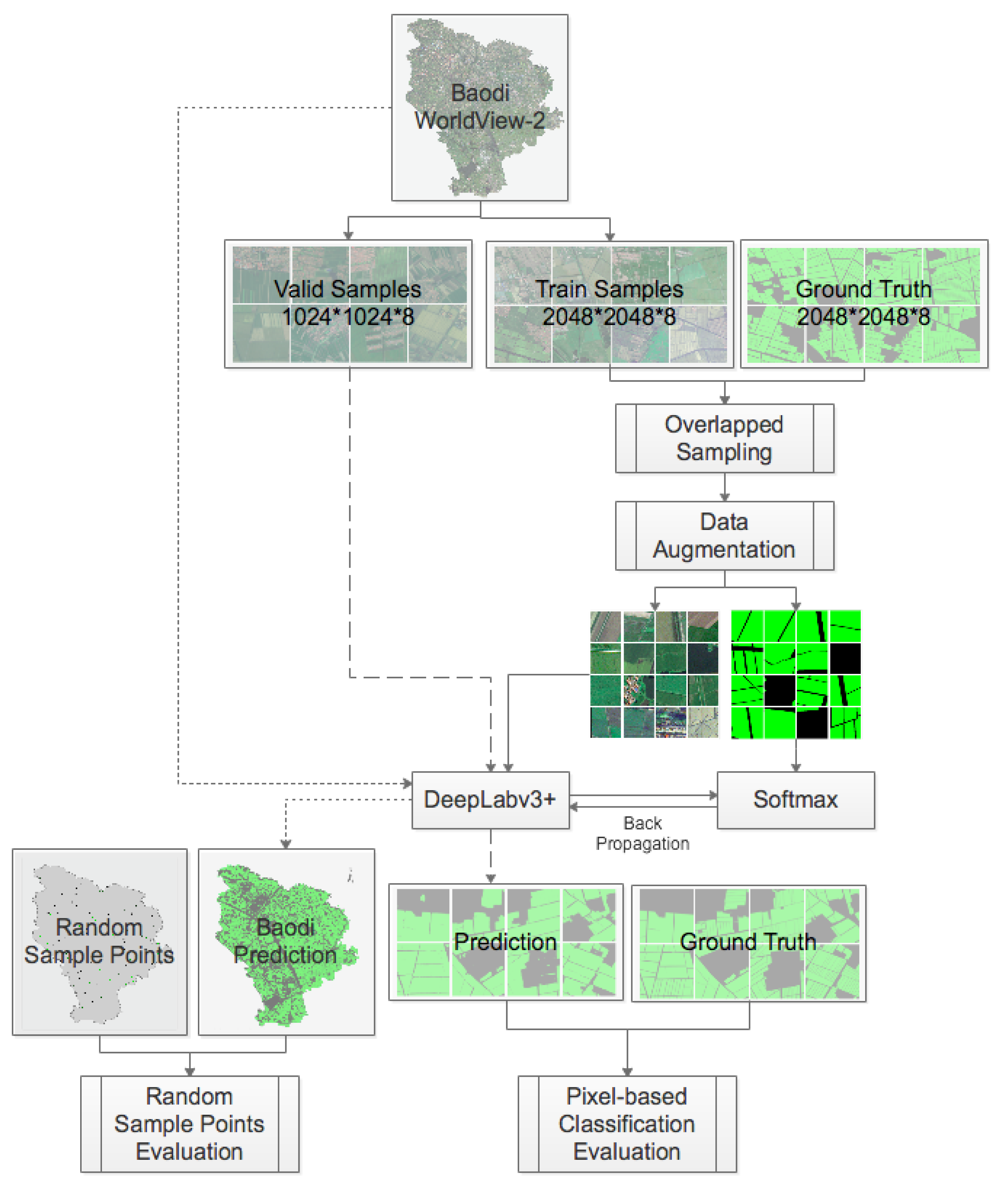
Figure 3.
DeepLabv3+ Architecture. (Conv = Convolutional layer).

Figure 4.
The eight validation (Val) slices with red-greed-blue (RGB) bands and their ground truth (GT) labels.
Figure 4.
The eight validation (Val) slices with red-greed-blue (RGB) bands and their ground truth (GT) labels.

Figure 5.
Classification results in Baodi with DeepLabv3+.

Figure 6.
Classification maps for U-Net (UNet), PspNet, SegNet, DeepLabv2 (DLv2), and DeepLabv3+ (DLv3+) on eight validation slices.
Figure 6.
Classification maps for U-Net (UNet), PspNet, SegNet, DeepLabv2 (DLv2), and DeepLabv3+ (DLv3+) on eight validation slices.


Figure 7.
Classification maps for Maximum Likelihood (ML), Support Vector Machine (SVM), RF (Random Forest) and DeepLabv3+ (DLv3+) on eight validation (Val) slices.
Figure 7.
Classification maps for Maximum Likelihood (ML), Support Vector Machine (SVM), RF (Random Forest) and DeepLabv3+ (DLv3+) on eight validation (Val) slices.


Figure 8.
The two WorldView-2 image slices with red-greed-blue (RGB) bands, and the results from the Global Map–Global LC (GLCNMO) and Finer Resolution Observation and Monitoring Global LC datasets (FROM-GLC) and our method.
Figure 8.
The two WorldView-2 image slices with red-greed-blue (RGB) bands, and the results from the Global Map–Global LC (GLCNMO) and Finer Resolution Observation and Monitoring Global LC datasets (FROM-GLC) and our method.

Table 1.
Parameters of Maximum Likelihood (ML), Support Vector Machine (SVM), and Random Forest (RF).
Table 1.
Parameters of Maximum Likelihood (ML), Support Vector Machine (SVM), and Random Forest (RF).
| Algorithm | Parameters |
|---|---|
| ML | Reject fraction (0.01) |
| A priori probability weighting (Equal) | |
| SVM | Cost or slack parameter (1.0) |
| Kernel type (RBF) | |
| Radial basis: gamma (1/3) | |
| RF | Number of trees (100) |
| Number of variables randomly sampled as candidates at each split (3) | |
| RBF: Radial-Based Function | |
Table 2.
Accuracy assessment of DeepLabv3+.
| Ground Truth | ||||
|---|---|---|---|---|
| Crop Area | Non-Crop Area | Sum | ||
| Mapped | Crop Area | 55 | 2 | 57 |
| Non-Crop Area | 3 | 40 | 43 | |
| Sum | 58 | 42 | 100 | |
| OA | 95% | |||
| KAPPA | 0.90 | |||
| * OA: Overall Accuracy | ||||
Table 3.
Comparisons of U-Net, PspNet, SegNet, DeepLabv2 (DLv2), and DeepLabv3+ (DLv3+) on pixel-wise classification.
Table 3.
Comparisons of U-Net, PspNet, SegNet, DeepLabv2 (DLv2), and DeepLabv3+ (DLv3+) on pixel-wise classification.
| Val | OA | KAPPA | ||||||||
|---|---|---|---|---|---|---|---|---|---|---|
| U-Net | PspNet | SegNet | DLv2 | DLv3+ | U-Net | PspNet | SegNet | DLv2 | DLv3+ | |
| 1 | 95.95% | 96.15% | 95.61% | 94.40% | 96.99% | 0.92 | 0.92 | 0.91 | 0.89 | 0.94 |
| 2 | 90.75% | 88.71% | 85.63% | 91.38% | 92.01% | 0.82 | 0.77 | 0.71 | 0.83 | 0.84 |
| 3 | 86.65% | 88.82% | 88.44% | 90.18% | 88.87% | 0.67 | 0.70 | 0.70 | 0.74 | 0.72 |
| 4 | 89.72% | 84.24% | 87.23% | 89.01% | 93.17% | 0.79 | 0.68 | 0.74 | 0.78 | 0.86 |
| 5 | 90.05% | 87.91% | 87.24% | 88.66% | 91.48% | 0.48 | 0.32 | 0.25 | 0.36 | 0.59 |
| 6 | 93.99% | 85.22% | 94.58% | 94.15% | 96.08% | 0.88 | 0.70 | 0.89 | 0.88 | 0.92 |
| 7 | 86.40% | 87.55% | 83.75% | 87.47% | 91.70% | 0.73 | 0.75 | 0.68 | 0.75 | 0.83 |
| 8 | 80.37% | 81.09% | 85.35% | 81.09% | 89.79% | 0.45 | 0.51 | 0.58 | 0.55 | 0.73 |
| AVG | 89.24% | 87.46% | 88.48% | 89.54% | 92.51% | 0.72 | 0.67 | 0.68 | 0.72 | 0.80 |
| Val: The number of the valid slices | OA: Overall Accuracy | |||||||||
| AVG: The average value of OA or kappa coefficient for the eight valid slices | ||||||||||
Table 4.
Comparisons of U-Net, PspNet, SegNet, DeepLabv2 (DLv2), and DeepLabv3+ (DLv3+) on pixel-wise classification.
Table 4.
Comparisons of U-Net, PspNet, SegNet, DeepLabv2 (DLv2), and DeepLabv3+ (DLv3+) on pixel-wise classification.
| Val | F1-SCORE (Crop Area) | F1-SCORE (Non-Crop Area) | ||||||||
|---|---|---|---|---|---|---|---|---|---|---|
| U-Net | PspNet | SegNet | DLv2 | DLv3+ | U-Net | PspNet | SegNet | DLv2 | DLv3+ | |
| 1 | 0.96 | 0.96 | 0.96 | 0.95 | 0.97 | 0.96 | 0.96 | 0.95 | 0.94 | 0.97 |
| 2 | 0.91 | 0.89 | 0.86 | 0.91 | 0.92 | 0.91 | 0.89 | 0.85 | 0.91 | 0.92 |
| 3 | 0.91 | 0.93 | 0.92 | 0.93 | 0.92 | 0.76 | 0.77 | 0.78 | 0.80 | 0.79 |
| 4 | 0.90 | 0.85 | 0.89 | 0.90 | 0.94 | 0.89 | 0.83 | 0.85 | 0.88 | 0.92 |
| 5 | 0.94 | 0.93 | 0.93 | 0.94 | 0.95 | 0.53 | 0.37 | 0.29 | 0.40 | 0.63 |
| 6 | 0.94 | 0.85 | 0.95 | 0.94 | 0.96 | 0.94 | 0.85 | 0.94 | 0.94 | 0.96 |
| 7 | 0.87 | 0.88 | 0.85 | 0.88 | 0.92 | 0.85 | 0.87 | 0.82 | 0.87 | 0.91 |
| 8 | 0.87 | 0.87 | 0.91 | 0.87 | 0.93 | 0.57 | 0.63 | 0.66 | 0.55 | 0.80 |
| AVG | 0.91 | 0.90 | 0.91 | 0.92 | 0.94 | 0.80 | 0.77 | 0.77 | 0.79 | 0.86 |
| Val: The number of the valid slices | ||||||||||
| AVG: The average value of F1-Score for the eight valid slices | ||||||||||
Table 5.
Comparisons of Maximum Likelihood (ML), Support Vector Machine (SVM), Random Forest (RF), and Convolutional Neural Networks (CNNs) on pixel-wise classification.
Table 5.
Comparisons of Maximum Likelihood (ML), Support Vector Machine (SVM), Random Forest (RF), and Convolutional Neural Networks (CNNs) on pixel-wise classification.
| Val | OA | KAPPA | ||||||
|---|---|---|---|---|---|---|---|---|
| ML | SVM | RF | CNNs | ML | SVM | RF | CNNs | |
| 1 | 80.90% | 79.77% | 71.49% | 95.82% | 0.61 | 0.59 | 0.43 | 0.92 |
| 2 | 72.11% | 71.34% | 69.51% | 89.70% | 0.44 | 0.43 | 0.39 | 0.79 |
| 3 | 85.42% | 77.63% | 63.02% | 88.59% | 0.57 | 0.39 | 0.20 | 0.71 |
| 4 | 66.70% | 64.87% | 62.81% | 88.67% | 0.31 | 0.28 | 0.25 | 0.77 |
| 5 | 81.69% | 81.56% | 66.00% | 89.07% | 0.09 | 0.16 | 0.10 | 0.40 |
| 6 | 73.06% | 72.42% | 65.90% | 92.80% | 0.46 | 0.44 | 0.32 | 0.85 |
| 7 | 67.98% | 70.70% | 69.51% | 87.37% | 0.37 | 0.43 | 0.40 | 0.75 |
| 8 | 56.58% | 59.05% | 56.35% | 83.54% | 0.08 | 0.13 | 0.13 | 0.56 |
| AVG | 73.06% | 72.17% | 65.57% | 89.45% | 0.37 | 0.36 | 0.28 | 0.72 |
| Val: The number of the valid slices | OA: Overall Accuracy | |||||||
| AVG: The average value of OA or kappa coefficient for the eight valid slices | ||||||||
Table 6.
Comparisons of Maximum Likelihood (ML), Support Vector Machine (SVM), Random Forest (RF), and Convolutional Neural Networks (CNNs) on pixel-wise classification.
Table 6.
Comparisons of Maximum Likelihood (ML), Support Vector Machine (SVM), Random Forest (RF), and Convolutional Neural Networks (CNNs) on pixel-wise classification.
| Val | F1-SCORE (Crop Area) | F1-SCORE (Non-Crop Area) | ||||||
|---|---|---|---|---|---|---|---|---|
| ML | SVM | RF | CNNs | ML | SVM | RF | CNNs | |
| 1 | 0.84 | 0.83 | 0.73 | 0.96 | 0.76 | 0.75 | 0.70 | 0.96 |
| 2 | 0.77 | 0.76 | 0.72 | 0.90 | 0.65 | 0.65 | 0.67 | 0.90 |
| 3 | 0.91 | 0.85 | 0.72 | 0.92 | 0.66 | 0.54 | 0.45 | 0.78 |
| 4 | 0.73 | 0.71 | 0.66 | 0.90 | 0.57 | 0.56 | 0.59 | 0.87 |
| 5 | 0.90 | 0.90 | 0.78 | 0.94 | 0.19 | 0.27 | 0.28 | 0.44 |
| 6 | 0.75 | 0.75 | 0.66 | 0.93 | 0.71 | 0.69 | 0.65 | 0.93 |
| 7 | 0.75 | 0.76 | 0.74 | 0.88 | 0.56 | 0.61 | 0.64 | 0.86 |
| 8 | 0.66 | 0.68 | 0.64 | 0.89 | 0.40 | 0.42 | 0.44 | 0.64 |
| AVG | 0.79 | 0.78 | 0.71 | 0.92 | 0.56 | 0.56 | 0.55 | 0.80 |
| Val: The number of the valid slices | ||||||||
| AVG: The average value of F1-Score for the eight valid slices | ||||||||
Table 7.
Accuracy assessment of the Global Map–Global LC (GLCNMO) and Finer Resolution Observation and Monitoring Global LC datasets (FROM-GLC) and our method.
Table 7.
Accuracy assessment of the Global Map–Global LC (GLCNMO) and Finer Resolution Observation and Monitoring Global LC datasets (FROM-GLC) and our method.
| GLCNMO | FROM-GLC | Our Method | |
|---|---|---|---|
| OA | 58% | 61% | 95% |
| KAPPA | 0.14 | 0.20 | 0.90 |
| OA: Overall Accuracy | |||
© 2019 by the authors. Licensee MDPI, Basel, Switzerland. This article is an open access article distributed under the terms and conditions of the Creative Commons Attribution (CC BY) license (http://creativecommons.org/licenses/by/4.0/).
Share and Cite
MDPI and ACS Style
Du, Z.; Yang, J.; Ou, C.; Zhang, T. Smallholder Crop Area Mapped with a Semantic Segmentation Deep Learning Method. Remote Sens. 2019, 11, 888. https://0-doi-org.brum.beds.ac.uk/10.3390/rs11070888
AMA Style
Du Z, Yang J, Ou C, Zhang T. Smallholder Crop Area Mapped with a Semantic Segmentation Deep Learning Method. Remote Sensing. 2019; 11(7):888. https://0-doi-org.brum.beds.ac.uk/10.3390/rs11070888
Chicago/Turabian StyleDu, Zhenrong, Jianyu Yang, Cong Ou, and Tingting Zhang. 2019. "Smallholder Crop Area Mapped with a Semantic Segmentation Deep Learning Method" Remote Sensing 11, no. 7: 888. https://0-doi-org.brum.beds.ac.uk/10.3390/rs11070888
Note that from the first issue of 2016, this journal uses article numbers instead of page numbers. See further details here.