Masi Entropy for Satellite Color Image Segmentation Using Tournament-Based Lévy Multiverse Optimization Algorithm


Abstract
:1. Introduction
2. Problem Statement
2.1. Summary Description of Multilevel Thresholding
2.2. Masi Entropy
3. Multiverse Optimization Algorithm
The Basic Multiverse Optimization Algorithm
Mathematical Model
| Algorithm 1 Pseudo-Code of the Traditional MVO Algorithm |
| 1 Initialize the positions of universes; |
| 2 Randomly initialize the population Sorted Universes (SU); |
| 3 While iteration < Max_iteration do |
| 4 For each universe indexed by i |
| 5 Check if any search agent goes beyond the search space and amend it; |
| 6 Calculate the objective function value of each universe (Inflation_rates of the universe)(NI); |
| 7 Update the best solution Best_universe, and WEP and TDR; |
| 8 For each object indexed by j |
| 9 Using Roulette Wheel Selection methods and the idea of wormhole, white hole, and black hole |
| to update the universe using Equation (10) |
| 10 Update the position of object in the optimal universe using Equation (11) |
| 11 End for |
| 12 End for |
| 13 End while |
4. The Proposed Multilevel Thresholding Algorithm
4.1. Selection Schemes
4.1.1. Roulette Wheel Selection
- Outstanding individuals will introduce a bias in the beginning of the search that may cause a premature convergence and a loss of diversity.
- If the fitness values of individuals in a group are very similar, the selection probability of the better and the worse individuals is very close, so it is difficult for the group to develop in a better direction.
- The algorithm procedure of roulette wheel selection depicted in Algorithm 2.
| Algorithm 2 Pseudo-Code of Roulette Wheel Selection |
| 1 Procedure: Roulette wheel selection |
| 2 While population size<pop_size do |
| 3 Generate pop_size random number r |
| 4 Calculate cumulative fitness, total fitness, total fitness(Pi) and sum of proportional fitness (Sum) |
| 5 Spin the wheel pop_size times |
| 6 If Sum < r then |
| 7 Select the first chromosome, otherwise, select j-th chromosome |
| 8 End If |
| 9 End While |
| 10 Return chromosomes with fitness value proportional to the size of selected wheel section |
| 11 End Procedure |
4.1.2. Tournament Selection
- Time complexity is more effective;
- Not susceptible to optimal biasing;
- Suitable for small populations, large populations will lose diversity and fall into local optimum;
- Relatively, slow convergence speed
| Algorithm 3 Pseudo-Code of Tournament Selection |
| 1 Procedure: Tournament Selection |
| 2 Determine the population size N |
| 3 Generate the number of selected individuals n |
| 4 If i < n then |
| 5 Generate fitness values (Fi) for a set of selected individuals |
| 6 End If |
| 7 Select the minimum value in Fi and its corresponding index i |
| 8 Returns the individual with the minimum fitness value |
| 9 End Procedure |
4.2. Lévy Flight
4.3. Tournament-Based Lévy Multiverse Optimization Algorithm
| Algorithm 4 Pseudo-Code of the Proposed Algorithm |
| 1 Initialize the positions of universes; |
| 2 Randomly initialize the population Sorted Universes (SU); |
| 3 While iteration < Max_iteration do |
| 4 For each universe indexed by i |
| 5 Check if any search agent goes beyond the search space and amend it; |
| 6 Calculate the reciprocal of the value of the objective function for each universe |
| (1/Inflation_rates of the universe)(1/NI); |
| 7 Update the best solution Best_universe, and WEP and TDR; |
| 8 For each object indexed by j |
| 9 Using Tournament Selection methods and the idea of wormhole, white hole, and black hole |
| to update the universe using Equation (10) |
| 10 Update the position of object in the optimal universe using Equation (19) |
| 11 End for |
| 12 End for |
| 13 End while |
4.4. The Proposed TLMVO-Based Multilevel Thresholding Method
5. The Computational Experiments and Results
5.1. Experimental Setup
- The traditional MVO algorithm [30];
- The state-of-the-art LMVO algorithm [37];
- An interesting bionic algorithm named ant lion algorithm (ALO) which can always find the maximum in the latest metaheuristics algorithm [56];
- A new complex swarm intelligent optimization technology, dragonfly algorithm (DA) [43];
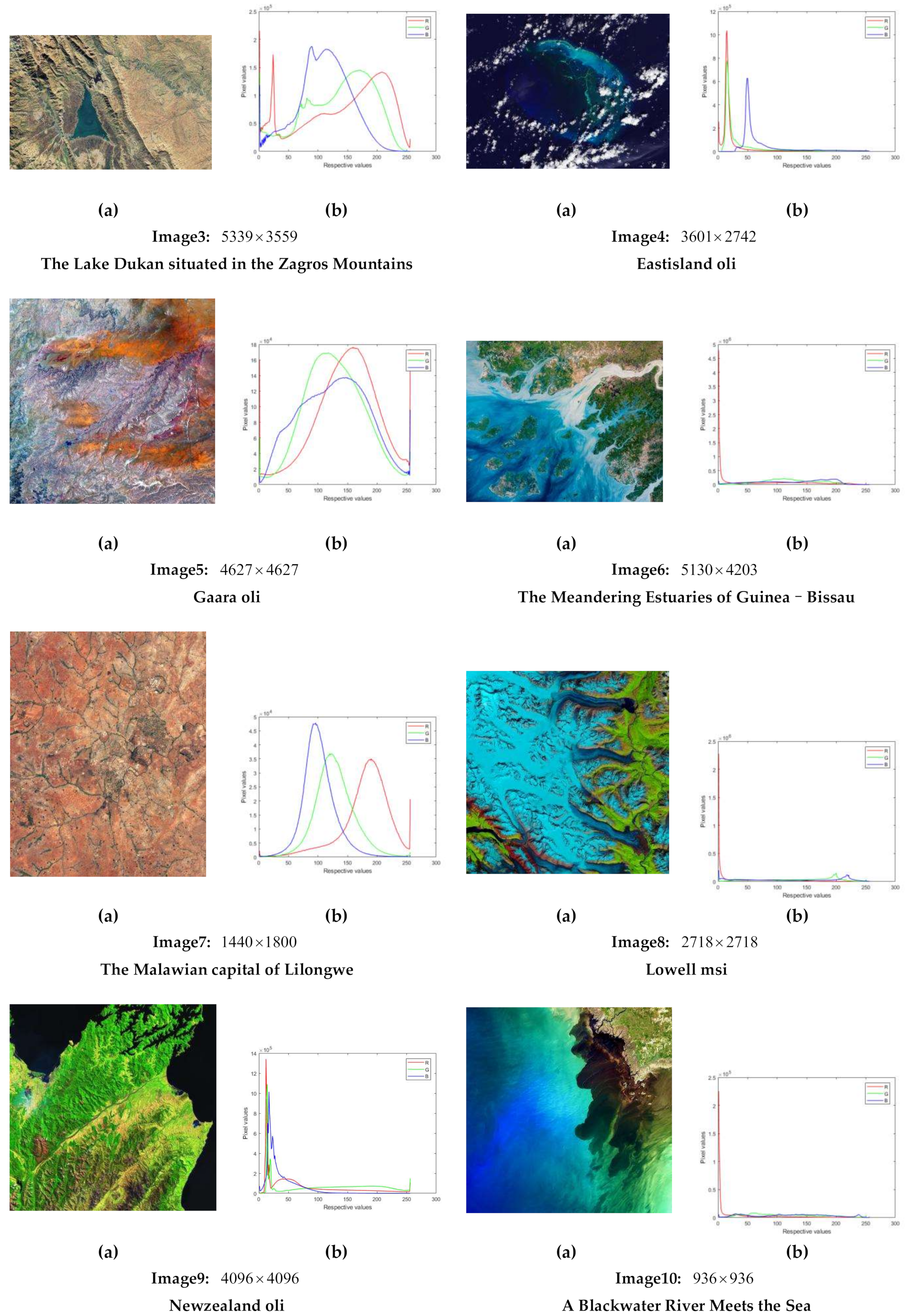
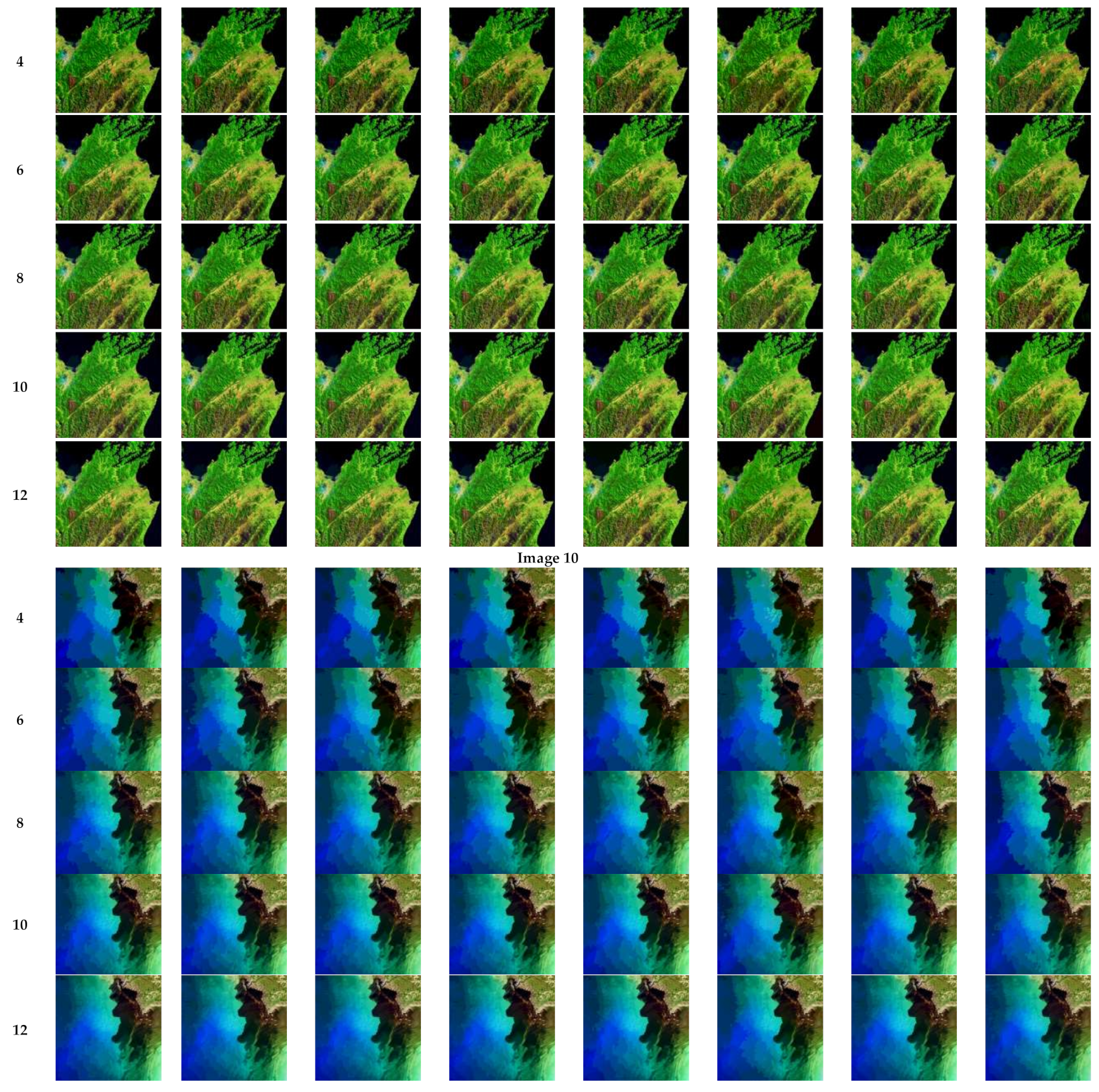
5.2. Satellite Color Image Used
5.3. Performance Metric
5.4. Implementation Results and Discussion
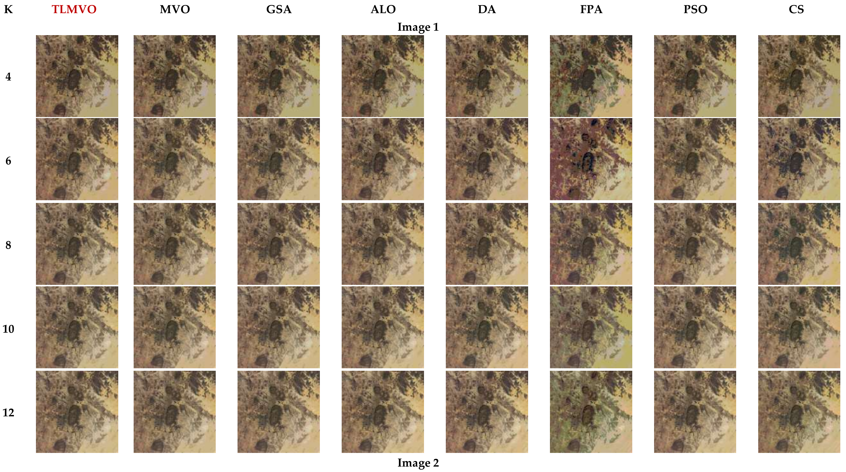
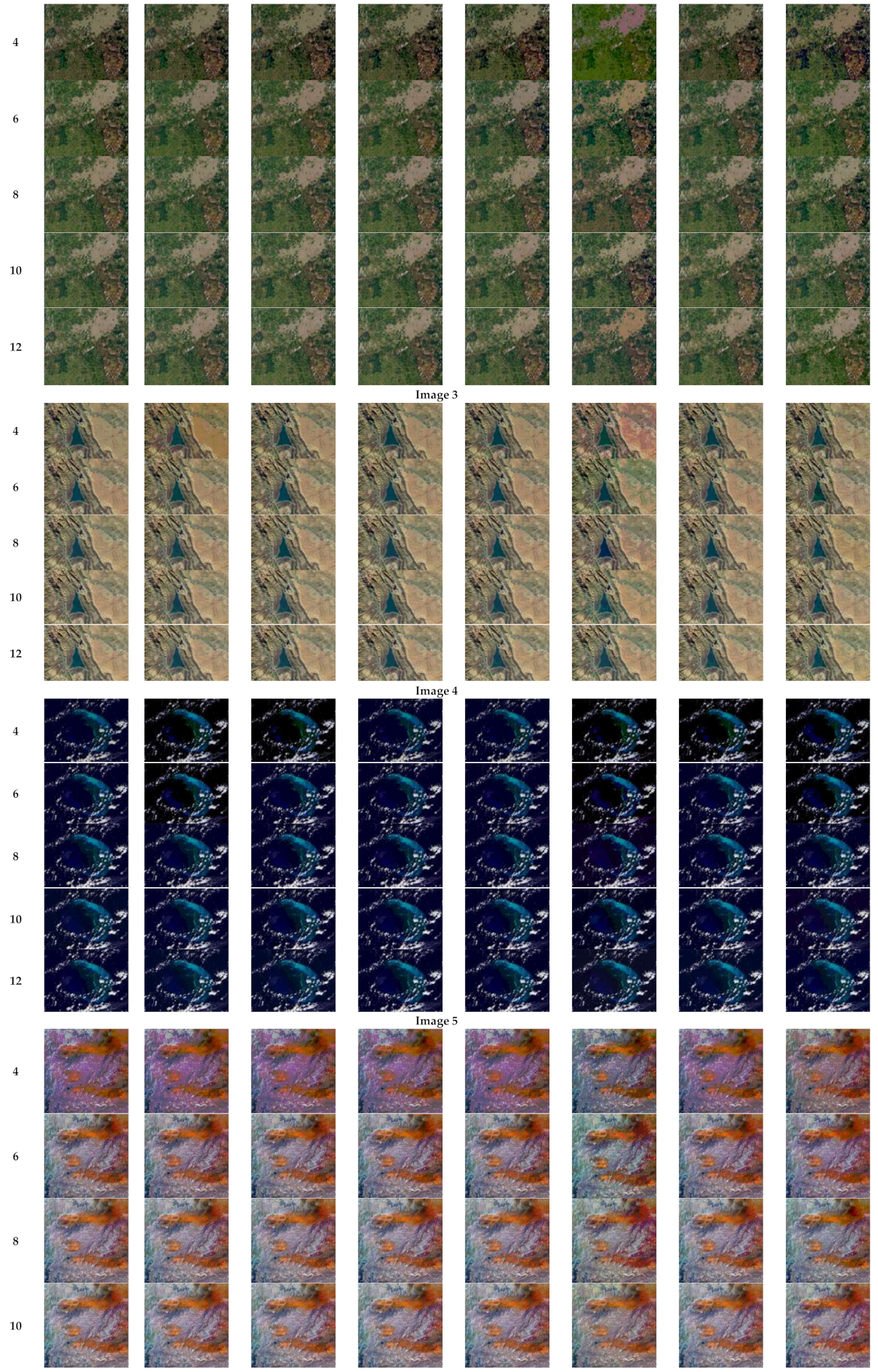
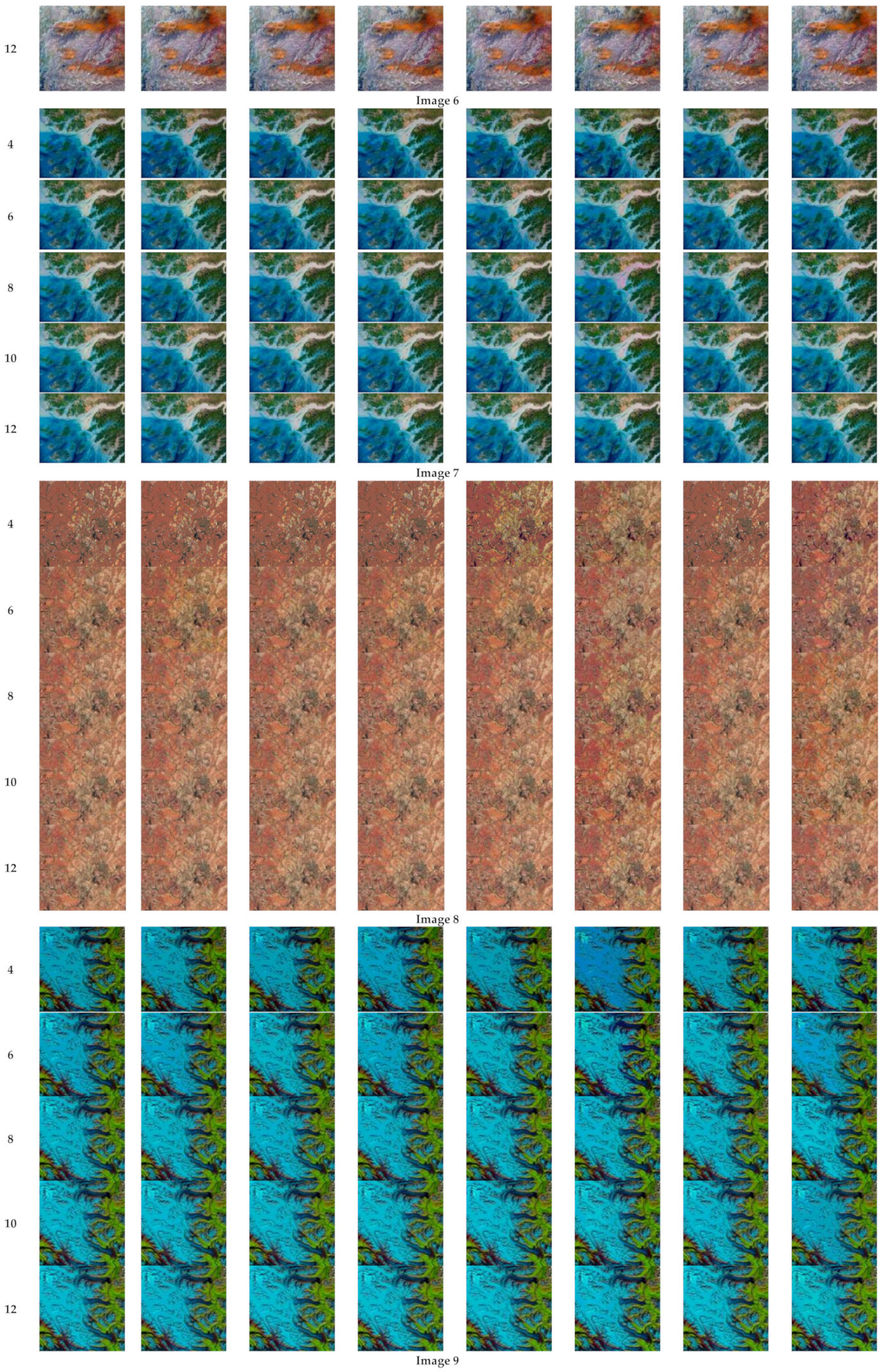
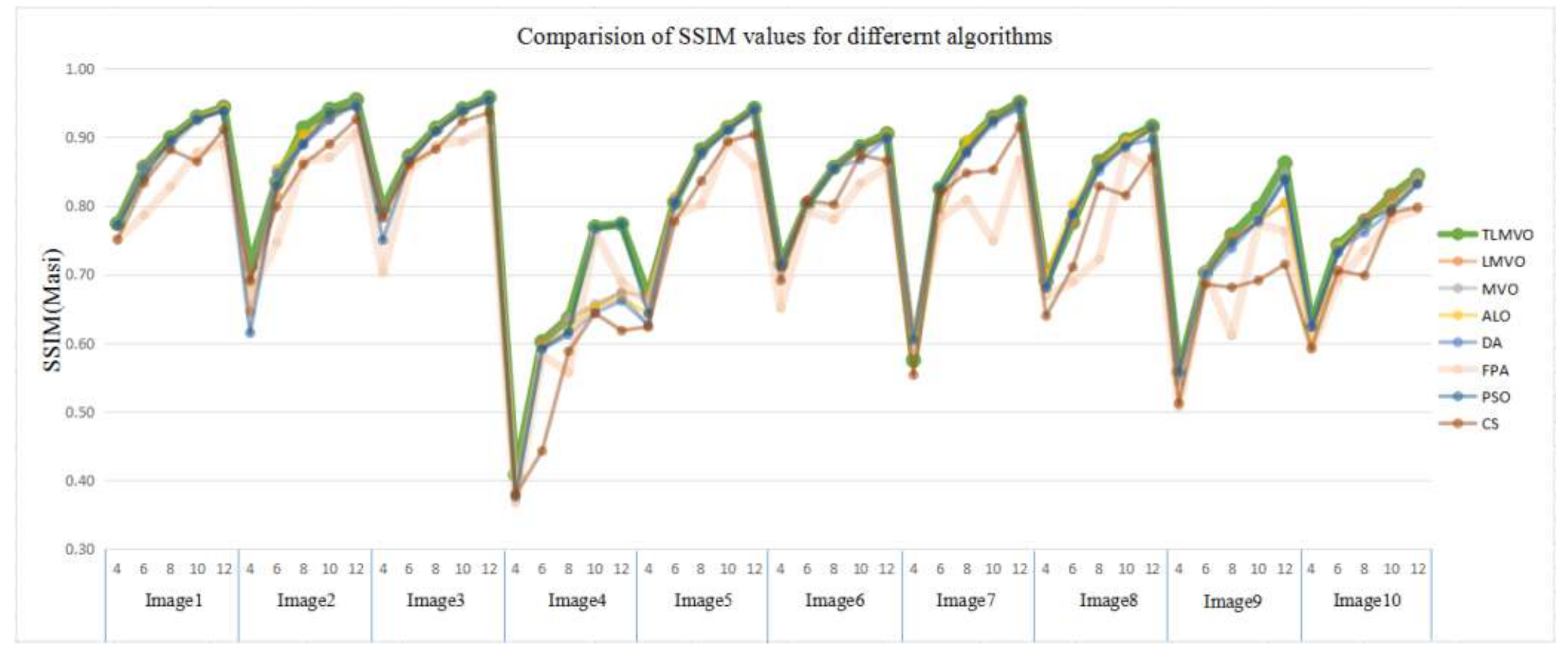
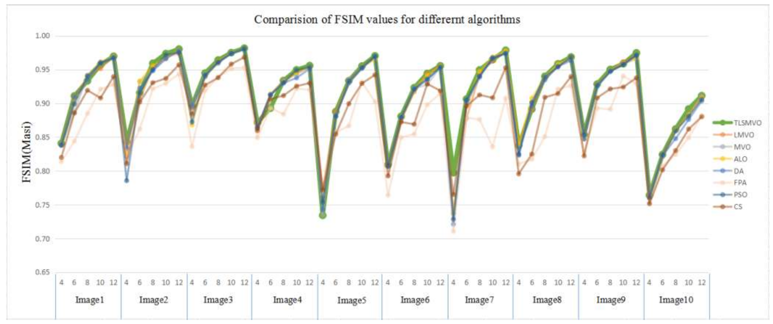
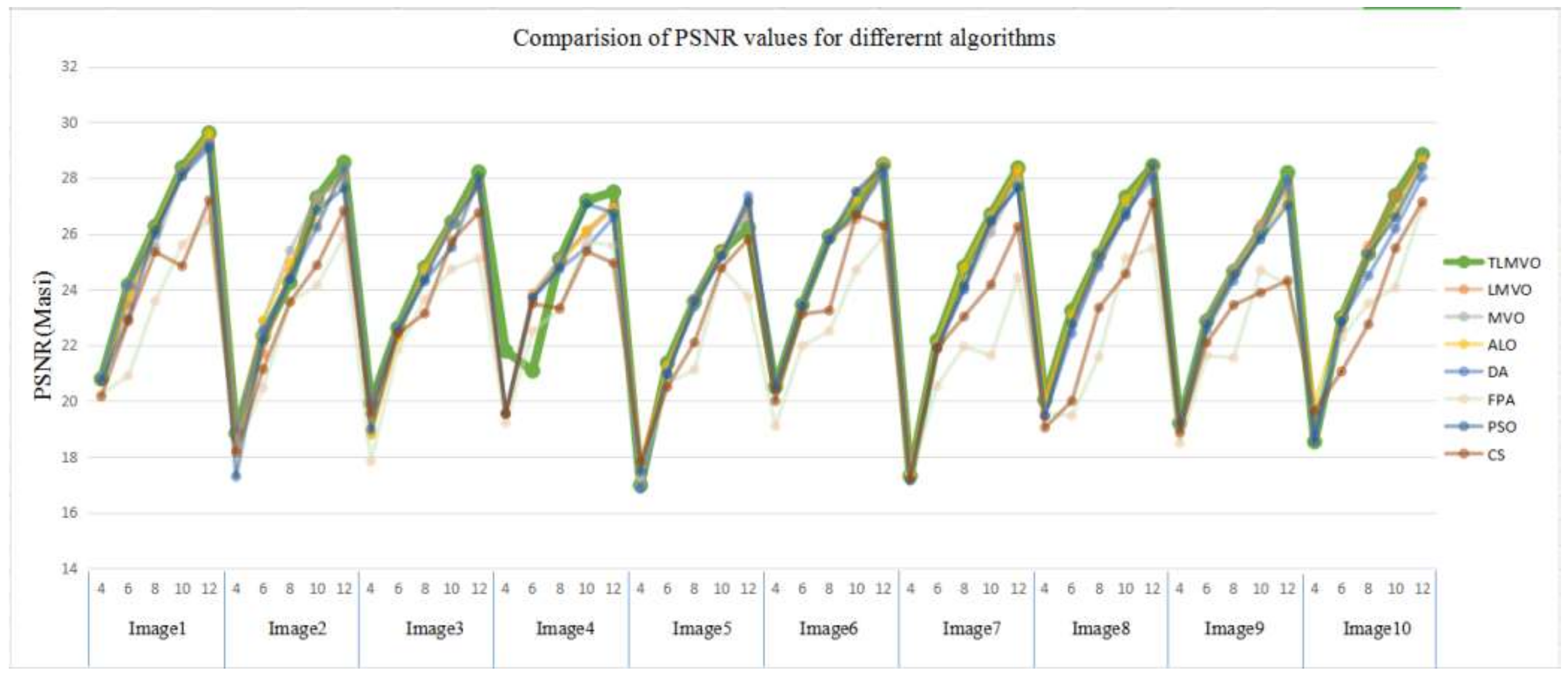
5.4.1. Image Segmentation Quality
- In the SSIM table: the values of Image 1 and Image 3 are all higher than the comparison algorithm;
- In the FSIM table: Image 3 and Image 6 yield excellence values compared with other algorithms in all cases;
- In the PSNR table: the values in Image 1, Image 3, and Image 8 are all much better than the comparative algorithms.
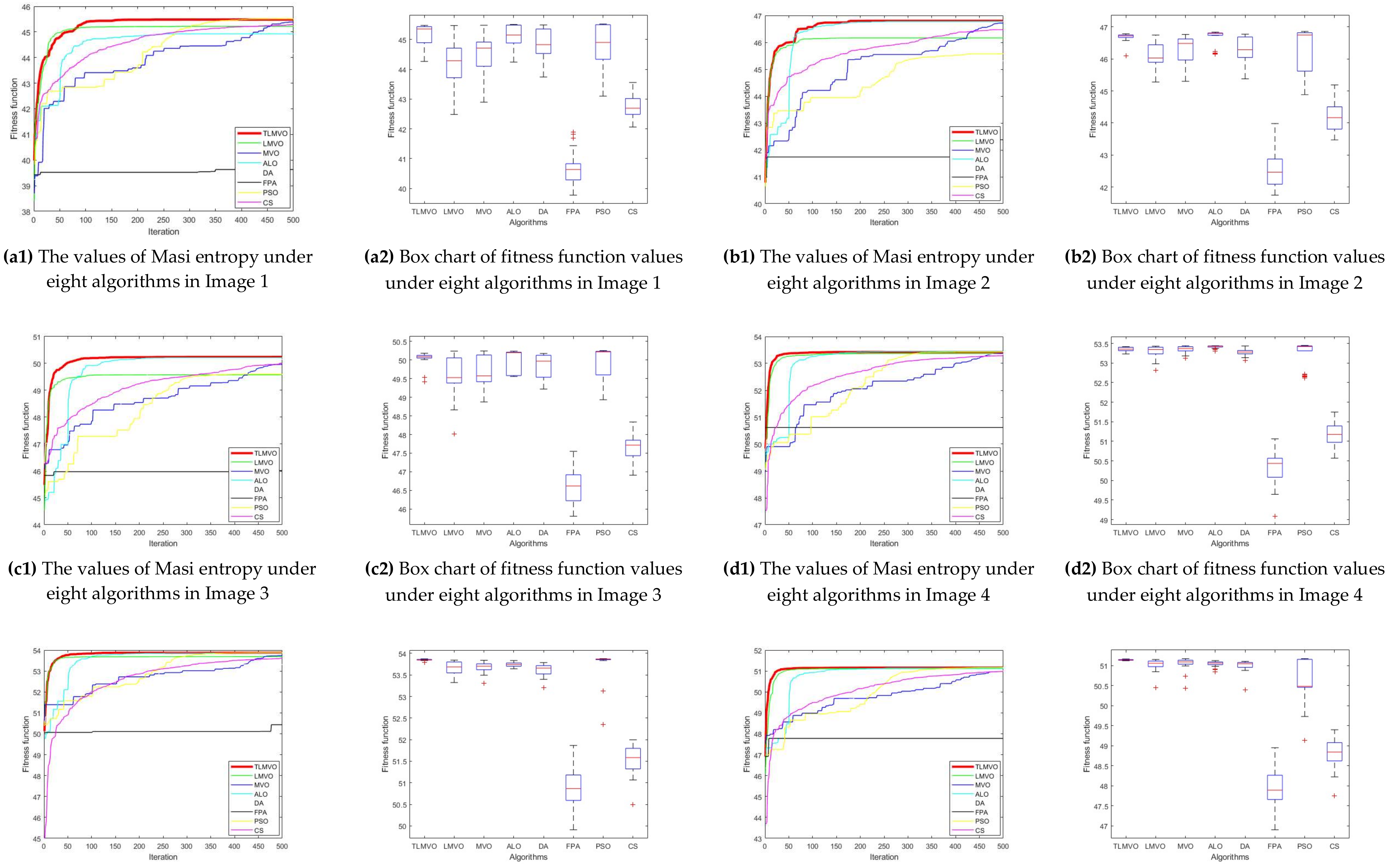
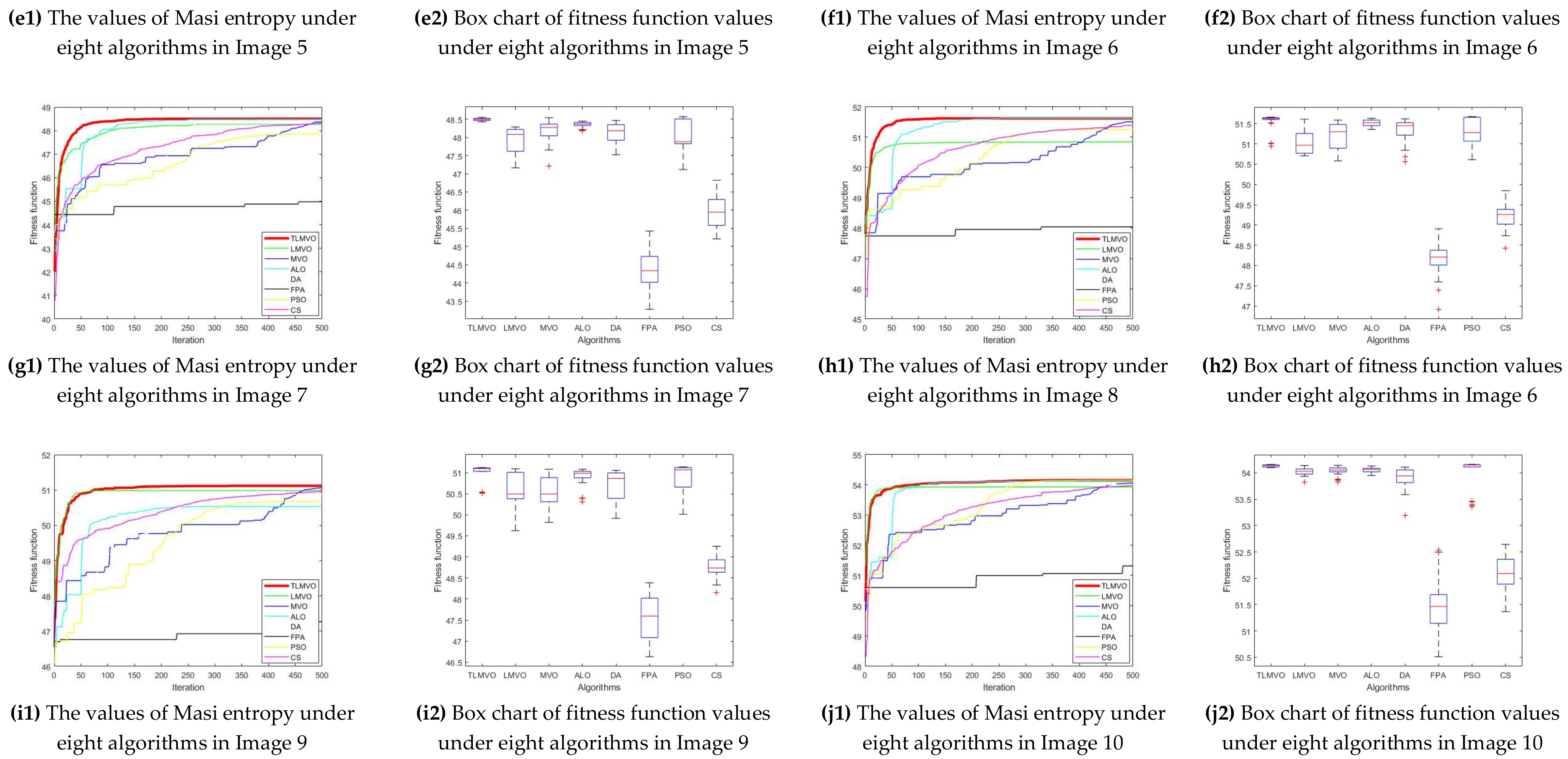
5.4.2. Fitness Function Value Analysis
5.4.3. Complexity Analysis
5.4.4. Statistical Analysis
6. Conclusions
Author Contributions
Funding
Acknowledgments
Conflicts of Interest
References
- Wang, A.; Zhang, W.; Wei, X. A review on weed detection using ground-based machine vision and image processing techniques. Comput. Electron. Agric. 2019, 158, 226–240. [Google Scholar] [CrossRef]
- Haindl, M.; Mikeš, S. A competition in unsupervised color image segmentation. Pattern Recognit. 2016, 57, 136–151. [Google Scholar] [CrossRef]
- Ayala, H.V.H.; Santos, F.M.D.; Mariani, V.C. Image thresholding segmentation based on a novel beta differential evolution approach. Expert Syst. Appl. 2015, 42, 2136–2142. [Google Scholar] [CrossRef]
- Bhandari, A.K.; Singh, V.K.; Kumar, A.; Singh, G.K. Cuckoo search algorithm and wind driven optimization based study of satellite image segmentation for multilevel thresholding using Kapur’s entropy. Expert Syst. Appl. 2014, 41, 3538–3560. [Google Scholar] [CrossRef]
- Mlakar, U.; Potočnik, B.; Brest, J. A hybrid differential evolution for optimal multilevel image thresholding. Exp. Syst. Appl. 2016, 65, 221–232. [Google Scholar] [CrossRef]
- Gao, H.; Kwong, S.; Yang, J.; Cao, J. Particle swarm optimization based on intermediate disturbance strategy algorithm and its application in multi-threshold image segmentation. Inf. Sci. 2013, 250, 82–112. [Google Scholar] [CrossRef]
- Bhandari, A.K.; Kumar, A.; Singh, G.K. Tsallis entropy based multilevel thresholding for colored satellite image segmentation using evolutionary algorithms. Expert Syst. Appl. 2015, 42, 8707–8730. [Google Scholar] [CrossRef]
- Ali, M.; Ahn, C.W.; Pant, M. Multilevel image thresholding by synergetic differential evolution. Appl. Soft Comput. 2014, 17, 1–11. [Google Scholar] [CrossRef]
- Mittal, H.; Saraswat, M. An optimum multilevel image thresholding segmentation using non-local means 2D histogram and exponential Kbest gravitational search algorithm. Eng. Appl. Artif. Intell. 2018, 71, 226–235. [Google Scholar] [CrossRef]
- Sezgin, M. Survey over image thresholding techniques and quantitative performance evaluation. J. Electron. Imaging 2004, 13, 146–168. [Google Scholar]
- Otsu, N. A threshold selection method from gray-level histograms. IEEE Trans. Syst. Man Cybern. 1979, 9, 62–66. [Google Scholar] [CrossRef]
- Mohamed, H.; Merzban, M.E. Efficient solution of Otsu multilevel image thresholding: A comparative study. Exp. Syst. Appl. 2019, 116, 299–309. [Google Scholar]
- Kapur, J.; Sahoo, P.K.; Wong, A.K. A new method forgray-level picture thresholding using the entropy of the histogram. CVGIP 1985, 29, 273–285. [Google Scholar]
- Hinojosa, S.; Dhal, K.G.; Elaziz, M.A.; Oliva, D.; Cuevas, E. Entropy-based imagery segmentation for breast histology using the Stochastic Fractal Search. Neurocomputing 2018, 321, 201–215. [Google Scholar] [CrossRef]
- Pal, S.K.; King, R.A.; Hashim, A.A. Automatic gray level thresholding through index of fuzziness and entropy. Pattern Recognit. Lett. 1983, 1, 141–146. [Google Scholar] [CrossRef]
- Sarkar, S. A differential evolutionary multilevel segmentation of near infra-red images using Renyi’s entropy. In Proceedings of the International Conference on Frontiers of Intelligent Computing: Theory and Applications (FICTA); Springer: Berlin/Heidelberg, Germany, 2013; Volume 199, pp. 699–706. [Google Scholar]
- Shannon, C.E. A mathematical theory of communication. MD Comput. 1997, 14, 306–317. [Google Scholar] [PubMed]
- Albuquerque, M.P.D.; Esquef, I.A.; Mello, A.R.G. Image thresholding using Tsallis entropy. Pattern Recognit. Lett. 2004, 25, 1059–1065. [Google Scholar] [CrossRef]
- Sumathi, R.; Venkatesulu, M.; Arjunan, S.P. Extracting tumor in MR brain and breast image with Kapur’s entropy based Cuckoo Search Optimization and morphological reconstruction filters. Biocybern. Biomed. Eng. 2018, 38, 918–930. [Google Scholar] [CrossRef]
- Lopez-Garcia, P.; Onieva, E.; Osaba, E. A metaheuristics based in the hybridization of Genetic Algorithms and Cross Entropy methods for continuous optimization. Expert Syst. Appl. 2016, 55, 508–519. [Google Scholar] [CrossRef]
- Pare, S.; Bhandari, A.K.; Kumar, A.; Singh, G.K. A new technique for multilevel color image thresholding based on modified fuzzy entropy and Lévy flight firefly algorithm. Comput. Electr. Eng. 2017, 70, 476–495. [Google Scholar] [CrossRef]
- Naidu, M.S.R.; Rajesh Kumar, P.; Chiranjeevi, K. Shannon and Fuzzy entropy based evolutionary image thresholding for image segmentation. Alex. Eng. J. 2017, 57, 1643–1655. [Google Scholar] [CrossRef]
- Masi, M. A step beyond Tsallis and Rényi entropies. Phys. Lett. 2005, 338, 217–224. [Google Scholar] [CrossRef]
- Kandhway, P.; Bhandari, A.K. A Water Cycle Algorithm-Based Multilevel Thresholding System for Color Image Segmentation Using Masi Entropy. Circuits Syst. Signal Process. 2018, 1–49. [Google Scholar] [CrossRef]
- Shubham, S.; Bhandari, A.K. A generalized Masi entropy based efficient multilevel thresholding method for color image segmentation. Multimed. Tools Appl. 2019, 1–42. [Google Scholar] [CrossRef]
- Wolpert, D.H.; Macready, W.G. No free lunch theorems for optimization. Trans. Evol. Comput. 1997, 1, 67–82. [Google Scholar] [CrossRef]
- Talbi, E.G. A taxonomy of hybrid metaheuristics. J. Heuristics 2002, 8, 541–564. [Google Scholar] [CrossRef]
- Baniani, E.A.; Chalechale, A. Hybrid PSO and genetic algorithm for multilevel maximum entropy criterion threshold selection. Int. J. Hybrid Inf. Technol. 2013, 6, 131–140. [Google Scholar] [CrossRef]
- Mafarja, M.M.; Mirjalili, S. Hybrid Whale Optimization Algorithm with simulated annealing for feature selection. Neurocomputing 2017, 260, 302–312. [Google Scholar] [CrossRef]
- Mirjalili, S.; Mirjalili, S.M. A Hatamlou, Multiverse Optimizer: A nature-inspired algorithm for global optimization. Neural Comput. Appl. 2016, 27, 495–513. [Google Scholar] [CrossRef]
- Ali, E.E.; El-Hameed, M.A.; El-Fergany, A.A.; El-Arini, M.M. Parameter extraction of photovoltaic generating units using multi-verse optimizer. Sustain. Energy Technol. Assess. 2016, 17, 68–76. [Google Scholar] [CrossRef]
- Jangir, P.; Parmar, S.A.; Trivedi, I.N.; Bhesdadiya, R.H. A novel hybrid Particle Swarm Optimizer with multi verse optimizer for global numerical optimization and Optimal Reactive Power Dispatch problem. Eng. Sci. Technol. Int. J. 2017, 20, 570–586. [Google Scholar] [CrossRef]
- Wang, X.; Luo, D.; Zhao, X.; Sun, Z. Estimates of energy consumption in China using a self-adaptive multi-verse optimizer-based support vector machine with rolling cross-validation. Energy 2018, 152, 539–548. [Google Scholar] [CrossRef]
- Elaziz, M.A.; Oliva, D.; Ewees, A.A.; Xiong, S. Multilevel thresholding-based grey scale image segmentation using multi-objective multi-verse optimizer. Expert Syst. Appl. 2019, 125, 112–129. [Google Scholar] [CrossRef]
- Noraini, M.; Geraghty, J. Genetic algorithm performance with different selection strategies in solving TSP. World Congr. Eng. 2011, II, 4–9. [Google Scholar]
- Medhane, D.V.; Sangaiah, A.K. Search space-based multi-objective optimization evolutionary algorithm. Comput. Electr. Eng. 2017, 58, 126–143. [Google Scholar]
- Jia, H.; Peng, X.; Song, W.; Lang, C.; Xing, Z.; Sun, K. Multiverse Optimization Algorithm Based on Lévy Flight Improvement for Multithreshold Color Image Segmentation. IEEE Access 2019, 7, 32805–32844. [Google Scholar] [CrossRef]
- Barrow, J.D.; Davies, P.C.W.; Harper, C.L. Science and Ultimate Reality: Quantum Theory, Cosmology and Complexity. Am. J. Phys. 2004, 74, 245–247. [Google Scholar]
- Khoury, J.; Ovrut, B.A.; Seiberg, N.; Steinhardt, P.J.; Turok, A.N. From big crunch to big bang. Phys. Rev. D 2001, 65, 381–399. [Google Scholar] [CrossRef]
- Yang, X.S.; Deb, S. Cuckoo Search via Lévy Flights. Mathematics 2010, 71, 210–214. [Google Scholar]
- Joshi, A.S.; Kulkarni, O. Cuckoo search optimization—A review. Sci. Direct Mater. 2017, 4, 7262–7269. [Google Scholar] [CrossRef]
- Yang, X.S. Flower pollination algorithm for global optimization. Unconv. Comput. Nat. Comput. 2012, 7445, 240–249. [Google Scholar]
- Shen, L.; Fan, C.; Huang, X. Multilevel image thresholding using modified flower pollination algorithm. IEEE Access 2018, 6, 30508–30518. [Google Scholar] [CrossRef]
- Xu, L.; Jia, H.; Lang, C.; Peng, X.; Sun, K. A novel method for multilevel color image segmentation based on dragonfly algorithm and differential evolution. IEEE Access 2019, 99, 2169–3536. [Google Scholar] [CrossRef]
- Goldberg, D.E.; Deb, K. A comparative analysis of selection schemes used in genetic algorithms. Found. Genet. Algorithms 1991, 1, 69–93. [Google Scholar]
- Handbook of Evolutionary Computation; IOP Publishing Ltd.: Bristol, UK; Oxford University Press: Oxford, UK, 1997.
- Blickle, T.; Thiele, L. A Comparison of Selection Schemes used in Genetic Algorithms. Evol. Comput. 1996, 4, 361–394. [Google Scholar] [CrossRef]
- Baker, J.E. Adaptive Selection Methods for Genetic Algorithms. In Proceedings of the First International Conference on Genetic Algorithms & Their Applications, Pittsburg, CA, USA, 24–26 July 1985. [Google Scholar]
- Li, J.; Tan, Y. Loser-Out Tournament-Based Fireworks Algorithm for Multimodal Function Optimization. IEEE Trans. Evol. Comput. 2017, 99. [Google Scholar] [CrossRef]
- Das, S.; Mallipeddi, R.; Maity, D. Adaptive evolutionary programming with p-best mutation strategy(Article). Swarm Evol. Comput. 2013, 9, 58–68. [Google Scholar] [CrossRef]
- Al-Betar, M.A.; Awadallah, M.A.; Khader, A.T.; Bolaji, A.L. Tournament-based harmony search algorithm for non-convex economic load dispatch problem. Appl. Soft Comput. 2016, 47, 449–459. [Google Scholar] [CrossRef]
- Ralf, M.; Klafter, J. The random walk’s guide to anomalous diffusion: A fractional dynamics approach. Phys. Rep. 2000, 339, 1–77. [Google Scholar]
- Dinkar, S.K.; Deep, K. An efficient opposition based Lévy Flight Antlion optimizer for optimization problems. Int. J. Comput. Sci. 2018, 29, 119–141. [Google Scholar] [CrossRef]
- Zhang, H.; Xie, J.; Hu, Q.; Shao, L.; Chen, T. A hybrid DPSO with Lévy flight for scheduling MIMO radar tasks. Appl. Soft Comput. 2018, 71, 242–254. [Google Scholar] [CrossRef]
- Jain, M.; Singh, V.; Rani, A. A novel nature-inspired algorithm for optimization: Squirrel search algorithm. Swarm Evol. Comput. 2019, 44, 148–175. [Google Scholar] [CrossRef]
- Mirjalili, S. The Ant Lion Optimizer. Adv. Eng. Softw. 2015, 83, 80–98. [Google Scholar] [CrossRef]
- Kennedy, J. Particle swarm optimization. In Proceedings of the ICNN’95 International Conference on Neural Networks, Perth, WA, Australia, 27 November–1 December 1995; Volume 4, pp. 1942–1948. [Google Scholar]
- Akay, B. A study on particle swarm optimization and artificial bee colony algorithms for multilevel thresholding. Appl. Soft Comput. 2013, 13, 3066–3091. [Google Scholar] [CrossRef]
- Liu, Y.; Mu, C.; Kou, W.; Liu, J. Modified particle swarm optimization-based multilevel thresholding for image segmentation. Soft Comput. 2015, 19, 1311–1327. [Google Scholar] [CrossRef]
- Gao, H.; Pun, C.M.; Kwong, S. An efficient image segmentation method based on a hybrid particle swarm algorithm with learning strategy. Inf. Sci. 2016, 369, 500–521. [Google Scholar] [CrossRef]
- Wang, M.; Wu, C.; Wang, L.; Xiang, D.; Huang, X. A feature selection approach for hyperspectral image based on modified ant lion optimizer. Knowl. Based Syst. 2019, 168, 39–48. [Google Scholar] [CrossRef]
- The Aerial Data Set. Available online: https://landsat.visibleearth.nasa.gov/view.php?id=144523 (accessed on 10 March 2019).
- Pare, S.; Kumar, A.; Bajaj, V.; Singh, G.K. An efficient method for multilevel color image thresholding using cuckoo search algorithm based on minimum cross entropy. Appl. Soft Comput. 2017, 61, 570–592. [Google Scholar] [CrossRef]
- Wang, Z.; Bovik, A.C.; Sheikh, H.R.; Simoncelli, E.P. Image quality assessment: From error visibility to structural similarity. IEEE Trans. Image Process. 2004, 13, 600–612. [Google Scholar] [CrossRef]
- Zhang, L.; Zhang, L.; Mou, X. FSIM: A Feature Similarity Index for Image Quality Assessment. IEEE Trans. Image Process. 2011, 20, 2378–2386. [Google Scholar] [CrossRef]
- Roy, R.; Laha, S. Optimization of stego image retaining secret information using genetic algorithm with 8-connected PSNR. Procedia Comput. Sci. 2015, 60, 468–477. [Google Scholar] [CrossRef]
- Pare, S.; Bhandari, A.K.; Kumar, A.; Singh, G.K. An optimal color image multilevel thresholding technique using grey-level co-occurrence matrix. Expert Syst. Appl. 2017, 87, 335–362. [Google Scholar] [CrossRef]
- Oliva, D.; Hinojosa, S.; Cuevas, E.; Pajares, G.; Avalos, O.; Gálvez, J. Cross entropy based thresholding for magnetic resonance brain images using Crow Search Algorithm. Expert Syst. Appl. 2017, 79, 164–180. [Google Scholar] [CrossRef]
- Ibrahim, R.A.; Elaziz, M.A.; Lu, S. Chaotic opposition-based grey-wolf optimization algorithm based on differential evolution and disruption operator for global optimization. Expert Syst. Appl. 2018, 108, 1–27. [Google Scholar] [CrossRef]
- Derrac, J.; García, S.; Molina, D.; Herrera, F. A practical tutorial on the use of nonparametric statistical tests as a methodology for comparing evolutionary and swarm intelligence algorithms. Swarm Evol. Comput. 2011, 1, 3–18. [Google Scholar] [CrossRef]


| Reference | Algorithm | Parameters | Value |
|---|---|---|---|
| [30] | MVO 1 | Mining capability | |
| Random parameters , , , | [0,1] | ||
| Contrast parameter | 0.5 | ||
| [37] | LMVO 1 | Lévy controlling constant | 1.5 |
| TLMVO 1 | Selection pressure | [0,1] | |
| Screening probability | [0,1] | ||
| [61] | ALO | Switch possibility | 0.5 |
| [44] | DA | Inertial weight | [0.5,0.9] |
| Seperation weight | [0,0.2] | ||
| Alignment weight | |||
| Cohesion weight | |||
| Maximum velocity | 25.5 | ||
| Food attraction weight | [0,2] | ||
| Enemy distraction weight | [0,0.1] | ||
| [43] | FPA | Switch possibility | 0.4 |
| Lévy controlling constant | 1.5 | ||
| [59] | PSO | Maximum inertia weight | 0.9 |
| Minimum inertia weight | 0.4 | ||
| Learning factors and | 2 | ||
| Maximum velocities | +120 | ||
| Minimum velocities | −120 | ||
| [7] | CS | Mutation probability value | 0.25 |
| Scale factor | 1.5 |
| Band No. | Name | Wavelength (μm) | Characteristics and Use |
|---|---|---|---|
| 1 | Visible blue | 0.45–0.52 | Maximum water penetration |
| 2 | Visible green | 0.52–0.60 | Good for measuring plant Vigor |
| 3 | Visible red | 0.63–0.69 | Vegetation discrimination |
| 4 | Near infrared | 0.76–0.90 | Biomass and shoreline Mapping |
| 5 | Middle Infrared | 1.55–1.75 | Moisture content of soil |
| 6 | Thermal Infrared | 10.4–12.5 | Soil moisture, thermal mapping |
| 7 | Middle Infrared | 2.08–2.35 | Mineral mapping |
| TEST IMAGES | K | TLMVO | LMVO | MVO | ALO | DA | FPA | PSO | CS | ||||||||||||||||
|---|---|---|---|---|---|---|---|---|---|---|---|---|---|---|---|---|---|---|---|---|---|---|---|---|---|
| R | G | B | R | G | B | R | G | B | R | G | B | R | G | B | R | G | B | R | G | B | R | G | B | ||
| 1 | 4 | 57 100 140 182 | 50 93 131 168 | 43 83 121 158 | 57 100 140 182 | 56 98 138 173 | 43 83 122 163 | 57 100 143 181 | 56 98 138 173 | 43 83 121 158 | 57 100 140 182 | 56 98 138 173 | 43 83 122 163 | 57 103 142 184 | 56 98 138 173 | 43 81 121 158 | 71 119 170 205 | 50 69 106 158 | 46 84 115 164 | 57 100 140 182 | 56 98 138 173 | 43 83 122 163 | 54 93 138 183 | 48 103 138 180 | 47 91 117 166 |
| 6 | 57 80 111 142 172 202 | 50 81 112 144 175 205 | 43 74 103 130 163 229 | 55 76 107 139 172 202 | 47 65 99 134 166 203 | 38 57 88 121 152 171 | 57 80 111 141 172 202 | 46 64 93 122 151 180 | 38 57 85 112 139 166 | 57 80 111 142 172 202 | 50 81 112 144 175 205 | 38 57 85 113 140 166 | 57 82 114 144 175 203 | 46 64 93 122 152 180 | 38 57 85 112 139 166 | 60 72 88 132 142 169 | 42 57 94 115 128 157 | 22 60 107 124 143 171 | 57 80 111 142 172 202 | 46 64 93 123 152 180 | 40 63 90 117 143 166 | 54 99 117 139 169 186 | 54 90 114 140 165 181 | 39 83 104 117 140 172 | |
| 8 | 54 70 94 119 145 172 200 227 | 37 50 66 90 114 138 160 183 | 38 55 77 100 123 148 167 230 | 46 64 82 103 127 150 177 203 | 46 61 84 107 131 155 180 205 | 38 49 67 88 109 130 152 171 | 55 72 94 117 139 162 184 206 | 46 59 80 102 127 152 180 205 | 38 52 71 91 112 133 154 171 | 46 64 84 108 132 156 180 206 | 46 63 87 110 134 157 181 205 | 38 53 72 92 113 134 155 171 | 54 70 94 118 141 164 186 208 | 43 57 78 98 120 155 180 205 | 38 53 74 95 116 136 155 171 | 47 51 70 84 120 147 191 212 | 35 43 54 66 93 122151 182 | 40 46 63 69 106 135 157 214 | 46 64 84 108 131 156 180 205 | 46 61 85 109 134 158 182 205 | 38 53 74 94 114 134 155 171 | 44 60 85 117 132 160 194 210 | 43 63 83 107 130 140 160 200 | 46 61 81 102 113 125 135 161 | |
| 10 | 46 57 67 81 99 117 135 156 179 205 | 41 56 71 89 107 125 144 163 183 205 | 38 52 68 85 103 120 137 155 171 184 | 46 63 79 97 115 133 152 171 189 208 | 37 50 63 82 101 120 140 161 182 205 | 33 46 64 85 107 129 154 171 206 208 | 46 63 77 93 112 131 151 170 189 208 | 41 56 68 84 102 118 136 158 181 205 | 33 46 60 77 94 110 123 138 155 171 | 46 64 80 97 115 133 151 171 191 210 | 41 56 71 90 108 127 145 164 183 205 | 33 46 58 74 91 107 124 141 156 171 | 55 72 91 112 132 151 171 189 207 227 | 41 56 70 88 106 120 137 160 183 206 | 38 49 65 80 96 111 126 141 156 171 | 39 53 81 97 97 107 127 160 188 206 | 40 50 71 82 97 119 140 154 190 227 | 25 40 51 60 74 100 101 127 147 176 | 46 64 82 104 126 146 167 187 206 227 | 41 56 71 89 107 125 144 163 184 205 | 33 46 59 74 90 106 122 139 155 171 | 44 54 62 88 99 115 157 168 193 210 | 39 52 61 77 92 101 126 135 159 167 | 30 39 66 73 79 109 123 136 146 164 | |
| 12 | 46 57 67 82 99 115 132 149 167 186 205 227 | 41 56 68 84 100 116 132 148 164 181 197 207 | 23 33 41 50 62 76 90 106 122 138 155 171 | 46 63 76 89 105 122 139 155 172 189 207 227 | 37 47 57 69 84 99 115 132 149 166 184 205 | 33 46 57 70 84 98 112 126 140 155 171 184 | 46 63 76 91 105 119 135 153 175 191 208 227 | 37 50 62 78 95 113 130 146 161 175 188 205 | 30 40 50 63 77 92 107 122 135 149 163 173 | 46 57 73 96 116 136 155 171 184 198 212 227 | 37 48 61 77 93 110 126 140 155 169 187 205 | 33 43 56 69 82 94 106 117 129 141 156 171 | 46 57 67 87 107 125 142 159 177 193 210 227 | 43 56 68 83 99 114 130 148 165 181 197 207 | 30 43 55 71 87 103 114 126 138 152 163 173 | 64 74 85 91 95 120 133 143 156 173 182 197 | 44 58 65 84 87 97 108 112 129 150 164 181 | 19 30 40 45 57 62 71 106 122 147 168 183 | 46 57 73 91 110 129 147 168 188 207 227 256 | 37 50 63 80 96 111 126 140 155 171 186 205 | 1 33 44 57 71 86 101 116 130 144 158 171 | 42 48 59 70 93 103 120 142 161 178 190 205 | 47 53 61 69 82 92 99 119 128 154 174 189 | 39 45 49 67 72 92 107 118 155 164 167 171 | |
| 2 | 4 | 60 117 174 197 | 38 80 123 170 | 33 88 141 170 | 60 117 174 197 | 59 117 157 187 | 33 88 141 170 | 50 88 126 182 | 38 111 157 187 | 44 89 141 170 | 50 88 126 182 | 59 117 157 187 | 33 88 141 170 | 50 89 126 182 | 63 117 157 187 | 33 88 141 177 | 67 84 116 195 | 64 115 164 213 | 58 95 138 178 | 58 95 138 178 | 38 111 157 187 | 33 88 141 170 | 41 77 120 179 | 58 117 157 184 | 51 94 148 187 |
| 6 | 30 61 94 127 174 197 | 38 63 93 124 158 187 | 19 46 88 135 158 193 | 43 81 121 172 190 212 | 38 61 91 123 157 187 | 19 46 88 135 157 181 | 35 69 105 137 174 197 | 38 6192 123 158 187 | 19 46 82 109 141 170 | 35 69 106 138 174 197 | 38 63 93 124 158 187 | 19 46 82 109 141 170 | 42 76 112 143 177 205 | 38 63 95 125 160 189 | 27 59 93 141 168 193 | 51 80 97 135 176 186 | 51 96 111 160 191 214 | 36 91 116 148 173 185 | 30 68 106 138 177 205 | 38 63 93 124 160 189 | 19 46 88 135 157 181 | 40 73 114 142 173 191 | 33 42 77 122 162 194 | 25 68 99 139 169 187 | |
| 8 | 23 50 79 112 141 172 190 212 | 36 55 78 103 127 155 174 202 | 19 44 75 101 135 157 177 197 | 18 42 68 94 120 147 177 205 | 36 57 81 105 128 157 179 208 | 19 46 78 103 135 157 177 203 | 23 46 71 95 120 146 177 205 | 36 56 80 104 127 155 174 202 | 17 33 57 83 108 136 157 181 | 30 61 90 118 145 172 190 212 | 38 59 83 106 130 157 177 208 | 17 34 59 85 109 136 157 185 | 39 66 95 120 146 172 190 212 | 36 58 82 107 130 157 179 208 | 19 46 76 101 133 149 170 193 | 42 69 100 123 134 149 186 212 | 39 45 80 105 133 166 208 211 | 25 33 46 56 90 139 160 195 | 30 58 87 117 144 172 190 212 | 38 59 83 107 130 157 177 208 | 19 46 78 102 133 149 170 197 | 19 61 75 104 119 142 170 190 | 37 59 91 108 138 160 178 203 | 18 35 71 98 127 144 161 194 | |
| 10 | 17 37 59 82 105 126 148 172 190 212 | 17 37 59 82 105 126 148 172 190 212 | 17 33 56 80 102 128 141 157 178 203 | 22 42 63 84 106 126 148 172 190 212 | 32 44 59 80 101 125 152 168 187 208 | 17 32 52 74 93 113 136 157 177 203 | 17 35 57 81 103 126 149 174 190 212 | 36 52 68 86 104 121 138 157 177 202 | 17 31 49 69 91 111 133 149 170 193 | 17 37 60 83 105 126 149 172 190 212 | 32 48 67 87 108 129 154 170 187 208 | 17 34 57 81 102 128 141 159 178 203 | 17 34 57 81 102 128 141 159 178 203 | 38 59 86 110 136 155 170 187 208 224 | 19 33 53 74 94 115 137 157 178 203 | 17 48 78 128 144 163 168 181 187 216 | 24 59 68 102 113 125 152 162 173 196 | 25 33 41 59 66 93 125 147 184 210 | 18 39 61 83 106 128 150 174 190 212 | 36 53 73 95 114 134 155 170 189 208 | 17 33 53 74 93 113 134 149 170 193 | 31 44 61 79 96 111 135 171 202 210 | 23 36 61 77 108 121 153 177 208 220 | 34 54 82 122 136 143 150 162 172 197 | |
| 12 | 9 22 37 54 70 88 107 126 149 174 190 212 | 26 38 53 72 91 112 132 154 169 187 202 218 | 17 32 50 70 89 108 128 141 157 175 193 210 | 9 22 36 52 74 97 121 145 169 182 197 212 | 26 38 52 66 83 101 119 135 154 168 187 208 | 11 25 39 58 82 103 127 141 157 172 191 208 | 17 30 47 68 87 105 123 139 153 172 190 212 | 26 38 53 69 86 104 121 136 153 168 187 208 | 11 19 32 50 73 92 111 131 145 164 181 203 | 17 35 55 72 93 110 132 151 170 182 197 212 | 32 44 61 78 95 113 130 149 160 174 189 210 | 17 31 46 63 79 96 113 131 144 160 179 203 | 17 34 53 72 89 107 124 138 153 174 190 212 | 36 50 65 80 97 119 139 155 170 187 205 220 | 17 28 44 60 78 96 116 133 145 160 179 203 | 5 4 58 64 83 114 138 146 173 197 221 239 | 32 72 85 98 101 126 152 171 174 182 209 227 | 20 26 46 61 76 92 112 119 137 143 167 191 | 11 28 47 66 84 102 120 137 154 174 190 212 | 26 38 53 69 86 103 120 137 155 170 189 210 | 17 32 48 66 82 99 115 134 149 170 197 256 | 19 54 78 90 109 118 135 175 184 200 212 237 | 17 32 56 67 90 105 125 138 160 168 175 194 | 19 41 62 71 77 83 102 116 131 142 157 166 | |
| 3 | 4 | 69 109 158 212 | 55 96 137 185 | 36 68 108 156 | 69 109 158 212 | 30 63 121 185 | 59 102 144 176 | 69 109 158 212 | 55 94 136 185 | 57 99 144 176 | 75 117 163 212 | 55 96 137 185 | 43 78 144 176 | 72 114 162 212 | 59 100 140 185 | 59 102 144 176 | 70 126 168 208 | 26 61 122 201 | 54 76 137 169 | 75 117 163 212 | 59 99 138 185 | 43 78 141 176 | 79 130 165 217 | 58 103 148 192 | 61 93 141 175 |
| 6 | 36 68 100 137 174 214 | 55 87 119 151 185 213 | 26 54 79 112 148 176 | 36 68 100 137 174 214 | 30 63 100 136 173 204 | 30 57 81 113 148 176 | 36 68 100 135 173 214 | 30 62 96 132 170 198 | 36 67 96 124 151 177 | 36 68 100 137 174 214 | 30 63 100 136 175 204 | 26 57 81 113 148 176 | 40 75 109 145 182 217 | 33 63 100 136 173 204 | 36 67 96 124 151 177 | 19 84 100 155 180 213 | 51 69 81 124 159 194 | 27 63 89 122 140 170 | 36 68 100 137 174 214 | 30 63 99 134 170 198 | 32 59 83 114 148 176 | 50 75 125 153 186 225 | 27 58 72 100 135 186 | 42 72 93 115 135 177 | |
| 8 | 16 39 69 99 130 161 193 221 | 19 40 63 92 121 149 180 204 | 19 39 59 79 104 129 153 177 | 34 62 86 112 140 170 206 231 | 19 40 63 92 121 151 185 213 | 24 47 70 93 116 141 163 181 | 35 62 87 117 146 176 209 231 | 30 61 85 111 138 165 189 213 | 24 46 68 92 116 141 163 181 | 35 65 93 121 150 179 209 231 | 30 61 87 112 138 165 189 213 | 24 47 70 93 117 141 163 181 | 16 40 70 100 135 169 206 231 | 30 61 86 112 138 165 189 213 | 25 49 72 96 119 143 163 181 | 14 76 110 131 164 178 202 232 | 9 37 52 81 104 136 182 203 | 27 54 74 84 106 130 142 192 | 16 43 75 106 139 172 206 231 | 30 61 87 115 142 170 192 213 | 24 46 68 91 116 141 163 181 | 12 55 90 100 148 175 205 223 | 23 68 104 137 153 171 197 214 | 44 71 110 122 137 149 165 177 | |
| 10 | 16 35 62 85 107 131 156 183 212 232 | 18 3 61 80 102 124 146 170 192 213 | 19 37 57 74 94 113 133 151 168 183 | 16 35 62 85 109 134 160 186 212 232 | 18 38 60 79 100 122 146 170 192 213 | 15 32 51 68 85 104 124 144 163 181 | 16 35 61 83 104 130 157 183 210 231 | 16 38 60 81 102 125 147 170 192 213 | 19 36 54 71 90 109 129 148 168 183 | 16 35 62 86 110 134 161 187 212 232 | 18 39 62 83 105 126 149 173 192 213 | 19 39 59 76 96 115 134 151 168 184 | 16 39 68 95 121 147 173 198 221 239 | 19 43 63 83 107 128 149 172 192 213 | 19 37 57 74 93 113 132 150 168 184 | 44 65 73 85 98 134 176 202 217 232 | 22 42 61 79 102 111 128 142 176 201 | 28 57 84 93 97 110 133 140 147 193 | 16 36 62 86 110 136 162 187 212 232 | 18 38 61 82 104 126 148 171 192 213 | 19 39 59 78 96 115 134 151 168 184 | 15 31 64 90 119 151 162 173 202 222 | 33 63 76 98 134 146 159 193 210 219 | 44 60 73 96 106 117 132 145 161 180 | |
| 12 | 16 32 50 68 86 106 125 145 166 188 212 231 | 18 38 59 76 93 110 127 144 162 180 196 213 | 18 35 52 68 83 99 115 131 148 163 176 187 | 16 32 50 68 86 107 128 149 170 191 212 231 | 14 30 48 63 79 96 113 131 149 171 192 213 | 15 29 45 61 78 96 114 132 151 168 183 246 | 16 30 46 65 83 100 119 138 159 182 210 231 | 18 36 52 66 84 103 121 139 158 178 196 213 | 15 32 51 65 80 96 112 128 146 163 176 187 | 16 34 55 75 97 117 139 159 180 202 221 239 | 18 38 60 79 97 114 131 149 168 186 204218 | 19 36 53 68 83 101 118 136 152 168 184 237 | 16 34 57 77 98 120 141 161 188 206 222 239 | 16 34 55 71 90 106 125 145 165 185 204 218 | 19 38 54 70 86 103 118 133 148 163 176 187 | 17 31 39 64 80 138 167 176 198 218 232 240 | 18 33 44 52 69 76 99 124 138 154 169 192 | 26 32 44 58 83 98 123 143 162 170 181 191 | 16 34 54 75 95 117 139 161 183 204 221 237 | 18 38 61 79 97 115 133 151 169 186 204 218 | 19 36 53 68 83 99 115 131 148 163 176 187 | 17 38 49 65 84 100 120 152 162 194 219 240 | 34 45 62 79 101 124 143 161 178 185 191 219 | 21 35 46 59 73 80 100 110 113 127 157 177 | |
| 4 | 4 | 35 80 135 195 | 36 83 140 197 | 40 77 124 180 | 35 80 135 195 | 34 74 128 190 | 77 119 169 212 | 35 80 135 195 | 34 74 128 190 | 77 119 169 212 | 35 80 135 195 | 36 83 140 197 | 77 119 169 212 | 35 80 141 199 | 34 74 128 192 | 77 119 169 212 | 38 103 157 195 | 31 83 165 195 | 77 134 167 204 | 35 80 135 195 | 36 83 140 197 | 77 119 169 212 | 37 69 124 195 | 40 79 134 186 | 72 108 165 223 |
| 6 | 25 61 103 141 179 217 | 34 71 106 142 179 217 | 61 88 119 151 184 219 | 25 58 94 134 174 215 | 31 62 93 128 167 208 | 40 65 95 133 174 214 | 25 61 103 141 178 216 | 34 69 104 140 176 216 | 40 65 95 133 176 216 | 25 58 95 135 175 215 | 34 71 106 142 180 218 | 40 65 95 133 176 216 | 25 61 103 141 179 217 | 34 71 111 147 183 220 | 40 65 96 135 180 217 | 26 61 107 148 200 212 | 24 50 88 121 181 220 | 32 92 141 173 200 234 | 25 61 103 141 179 217 | 34 71 106 142 179 217 | 40 65 95 133 174 215 | 23 68 99 137 167 218 | 27 66 105 156 181 208 | 36 61 95 123 152 196 | |
| 8 | 23 46 73 103 133 164 195 225 | 24 47 73 103 132 162 193 224 | 40 63 88 115 144 174 200 228 | 23 46 73 104 134 164 194 225 | 24 47 73 103 132 162 193 224 | 40 63 88 117 145 174 200 227 | 23 46 72 103 131 159 190 223 | 24 47 73 103 132 162 194 225 | 40 63 88 115 145 174 200 228 | 22 43 72 104 135 166 196 226 | 31 58 84 112 140 168 197 225 | 40 63 88 116 142 169 197 226 | 24 50 80 111 142 171 199 227 | 31 62 89 117 144 175 203 232 | 40 63 88 117 146 174 201 229 | 49 66 85 113 144 156 179 194 | 34 71 106 141 149 172 183 218 | 28 46 90 97 110 153 196 224 | 23 46 73 104 134 164 195 225 | 31 58 84 112 140 168 197 227 | 40 63 88 115 142 169 199 226 | 25 36 63 99 133 159 211 232 | 35 55 63 107 139 166 207 236 | 35 81 116 140 169 187 221 238 | |
| 10 | 22 40 60 82 104 125 148 174 200 228 | 10 31 55 78 103 128 154 179 205 231 | 26 41 57 76 96 119 142 169 195 223 | 22 43 70 94 118 140 163 186 208 231 | 24 47 71 93 116 140 162 185 208 232 | 26 41 60 81 103 126 151 176 200 227 | 22 42 61 83 105 129 152 176 202 230 | 22 39 62 83 106 129 154 177 202 229 | 40 58 77 96 118 140 162 184 207 229 | 23 43 70 94 118 141 163 187 209 233 | 23 43 67 91 115 138 162 185 208 232 | 26 41 60 84 107 129 152 176 201 229 | 22 43 70 95 119 142 164 187 210 233 | 23 44 69 92 117 140 162 184 208 232 | 41 65 92 121 145 169 189 206 223 240 | 7 26 46 66 84 136 146 179 206 240 | 10 24 56 89 102 116 124 167 200 216 | 23 40 93 113 144 149 176 183 207 235 | 22 42 63 84 107 132 158 182 206 231 | 9 24 47 73 102 128 154 180 206 231 | 26 41 60 84 107 129 152 176 202 229 | 21 41 58 68 79 103 138 166 174 191 | 24 41 72 127 160 178 188 206 221 246 | 27 45 69 86 109 141 161 174 196 230 | |
| 12 | 22 40 61 82 103 121 141 160 179 198 217 237 | 9 22 38 58 78 99 119 140 162 185 208 232 | 40 58 77 95 113 132 151 169 184 201 218 236 | 21 35 52 71 91 110 130 151 171 191 212 234 | 22 39 59 78 98 118 139 159 178 197 216 236 | 26 41 56 76 94 113 133 153 174 194 214 234 | 21 37 54 72 90 108 129 149 170 191 212 234 | 22 38 55 73 91 110 129 149 169 191 212 234 | 26 41 56 75 93 111 131 151 173 193 213 234 | 22 42 61 80 100 119 139 159 178 198 218 237 | 23 41 60 80 100 119 139 159 178 198 217 237 | 26 41 56 73 89 108 127 147 169 191 212 234 | 22 40 61 82 104 127 149 169 188 206 224 240 | 23 41 62 82 102 121 140 160 179 199 219 238 | 26 41 59 79 101 124 151 176 198 216 230 242 | 14 35 50 72 86 90 137 163 176 188 204 222 | 52 73 86 96 113 131 152 164 185 192 212 222 | 20 34 50 54 74 80 94 129 144 162 214 238 | 22 42 61 80 100 119 139 158 178 199 219 239 | 9 23 41 62 83 105 126 147 168 191 213 234 | 1 26 41 60 80 102 124 147 169 190 212 233 | 33 43 56 92 111 126 133 149 156 176 211 226 | 25 48 91 112 127 146 171 193 203 225 233 246 | 17 36 61 74 105 113 135 153 170 183 200 221 | |
| 5 | 4 | 54 88 139 203 | 46 86 169 217 | 64 121 189 226 | 43 88 139 203 | 53 103 173 217 | 62 116 170 215 | 54 88 139 203 | 46 86 169 217 | 64 121 189 226 | 46 88 139 203 | 53 104 175 217 | 64 121 189 226 | 57 100 171 214 | 48 98 169 217 | 65 124 189 226 | 54 104 172 205 | 52 118 175 226 | 54 118 171 221 | 54 88 139 203 | 53 104 175 217 | 64 121 189 226 | 47 89 137 212 | 58 111 165 217 | 84 131 179 224 |
| 6 | 34 68 101 142 187 223 | 39 77 117 159 195 221 | 34 73 113 154 194 226 | 43 85 118 158 196 224 | 38 72 112 155 192 220 | 34 73 113 154 194 226 | 34 65 100 140 187 223 | 38 72 112 155 192 220 | 38 74 114 154 194 226 | 34 68 101 139 180 214 | 39 75 114 155 192 220 | 38 76 116 156 194 226 | 34 69 103 143 187 223 | 39 77 117 159 195 221 | 34 73 116 156 194 226 | 50 86 105 126 181 210 | 28 55 75 119 153 206 | 33 52 71 118 159 210 | 34 65 100 141 187 223 | 39 77 117 159 195 221 | 38 76 116 156 194 226 | 44 80 128 160 205 235 | 55 91 127 169 199 234 | 35 77 109 132 198 228 | |
| 8 | 29 57 86 112 143 175 202 227 | 26 48 74 102 132 165 195 221 | 24 56 86 116 147 178 205 227 | 34 61 88 115 145 175 202 227 | 26 52 79 110 141 173 202 226 | 22 51 81 112 142 173 203 227 | 34 58 88 116 144 175 203 232 | 26 48 76 102 130 164 195 221 | 22 50 78 108 140 172 203 226 | 29 57 86 111 142 175 202 227 | 26 52 79 114 145 175 202 226 | 34 62 90 119 149 179 205 227 | 29 58 88 116 147 178 203 228 | 26 53 83 116 150 181 206 234 | 24 56 87 119 148 178 205 227 | 23 46 75 118 144 180 217 227 | 29 61 74 119 151 194 230 239 | 35 89 106 157 182 196 210 234 | 29 58 88 116 145 175 202 227 | 26 53 82 114 147 178 206 234 | 24 56 85 114 144 174 203 227 | 26 46 79 101 140 169 203 231 | 18 35 50 85 112 149 185 221 | 31 54 93 107 156 187 205 231 | |
| 10 | 21 43 65 88 111 138 165 190 214 235 | 26 45 65 90 116 142 169 195 215 234 | 18 39 63 87 111 135 160 186 208 231 | 20 43 65 88 110 135 161 187 209 232 | 22 39 61 82 106 134 161 188 213 234 | 15 34 59 83 108 133 159 186 208 231 | 21 43 65 88 108 130 153 180 203 230 | 25 43 63 85 112 140 165 191 213 234 | 17 38 60 83 106 130 157 184 208 231 | 21 43 65 88 112 139 165190 212 235 | 26 48 73 97 121 146 167 192 213 234 | 18 41 65 90 115 140 165 191 213 232 | 30 57 85 107 130 155 178 201 221 239 | 26 48 75 102 128 153 178 198 217 238 | 18 43 71 99 127 154 176 198 215 235 | 29 52 78 112 126 131 161 176 204 222 | 42 75 93 106 114 128 145 176 227 244 | 8 32 61 71 97 124 153 188 216 229 | 21 43 65 88 112 138 165 190 214 235 | 26 48 73 98 123 149 175 198 217 234 | 18 39 64 89 114 139 163 188 210 231 | 6 26 64 89 116 142 150 175 204 224 | 48 66 80 88 113 143 151 184 206 230 | 18 43 54 98 113 136 154 165 187 213 | |
| 12 | 18 34 54 71 88 109 132 155 180 202 223 239 | 25 43 63 84 106 129 152 175 195 213 226 242 | 11 22 37 53 72 92 114 137 162 186 208 231 | 14 29 43 60 77 93 112 133 154 178 203 232 | 25 42 61 81 102 123 143 163 182 202 219 238 | 17 34 54 74 94 114 135 155 176 196 215 235 | 19 36 54 69 88 107 129 151 174 195 214 235 | 22 38 55 75 94 120 139 158 177 196 215 234 | 11 28 47 65 86 105 127 148 171 194 213 231 | 21 42 61 80 99 119 140 161 182 203 223 240 | 25 43 63 83 103 123 143 164 183 202 217 234 | 17 34 53 72 91 112 133 153 172 194 213 232 | 28 47 65 85 103 121 139 159 180 198 216 235 | 26 43 64 83 99 115 135 155 175 195 217 238 | 17 38 60 83 107 130 150 169 186 203 218 235 | 14 47 66 80 97 127 147 188 208 220 224 246 | 31 47 63 81 100 114 125 165 185 205 226 247 | 16 33 77 87 101 119 130 142 157 213 229 238 | 21 43 62 82 101 121 141 161 181 202 223 240 | 25 39 55 76 97 117 138 159 179198 217 234 | 14 34 53 73 94 114 134 154 174 194 215 235 | 36 49 59 84 112 122 129 153 170 196 229 241 | 21 31 66 80 101 124 142 156 185 193 219 246 | 42 52 77 97 117 137 167 175 188 196 207 234 | |
| 6 | 4 | 25 75 127 175 | 45 81 128 170 | 38 84 129 172 | 25 75 127 175 | 45 81 128 170 | 38 84 129 172 | 25 75 127 175 | 45 81 129 172 | 38 84 129 172 | 25 75 127 175 | 45 81 129 172 | 38 84 129 172 | 25 75 127 175 | 45 81 130 175 | 38 34 129 172 | 37 95 137 173 | 35 54 122 158 | 27 82 118 173 | 25 75 127 175 | 45 81 129 172 | 38 84 129 172 | 24 81 123 169 | 47 72 132 173 | 42 84 128 174 |
| 6 | 16 54 90 12 163 197 | 42 68 98 129 159 192 | 27 56 87 118 149 182 | 16 53 89 127 163 197 | 40 63 93 127 159 192 | 22 51 83 116 149 182 | 16 52 88 126 163 197 | 42 68 97 128 158 192 | 27 56 87 118 149 182 | 16 54 91 128 163 197 | 42 68 98 129 159 192 | 27 56 87 118 149 182 | 20 59 96 133 168 199 | 42 70 99 129 159 192 | 27 56 87 119 151 183 | 6 50 95 124 177 218 | 50 72 88 108 144 169 | 16 53 73 96 119 155 | 16 54 91 128 163 197 | 42 68 98 129 159 192 | 26 56 87 118 149 182 | 16 33 62 91 131 190 | 32 64 90 116 147 179 | 35 68 82 104 133 171 | |
| 8 | 15 41 67 94 121 147 174 202 | 37 58 79 102 126 149 172 195 | 13 35 59 85 110 136 162 189 | 15 45 75 105 136 168 197 226 | 34 52 74 96 119 143 167 193 | 21 43 68 93 118 143 168 193 | 15 40 66 92 119 146 173 202 | 36 54 75 99 124 147 170 194 | 21 43 67 90 114 139 165 190 | 15 41 68 95 122 148 175 202 | 37 54 75 99 124 146 169 193 | 21 4 67 91 116 140 165 190 | 15 41 70 98 125 152 177 204 | 40 59 80 103 126 148 171 194 | 21 43 68 92 117 141 167 193 | 24 48 64 97 137 189 200 224 | 18 40 65 89 106 111 122 171 | 26 58 86 150 162 191 206 221 | 15 41 68 95 122 148 175 202 | 40 59 80 103 126 149 172 195 | 21 43 68 93 118 143 168 193 | 16 44 85 102 125 175 186 211 | 48 87 102 127 159 172 184 204 | 26 47 62 83 100 117 130 183 | |
| 10 | 10 27 46 64 85 109 135 162 187 212 | 34 52 71 90 109 128 148 168 188 207 | 13 31 48 68 89 110 131 157 184 219 | 12 32 52 74 95 117 143 170 197 226 | 32 45 59 74 92 113 135 158 189 218 | 13 31 50 71 92 114 136 160 186 219 | 12 33 54 76 99 121 143 166 187 210 | 34 47 63 80 98 118 138 157 176 196 | 13 31 51 71 91 111 133 154 175 197 | 13 36 59 82 104 126 148 170 191 214 | 34 52 72 92 113 134 154 173 195 219 | 13 31 51 74 95 116 137 157 177 198 | 16 46 78 102 127 148 170 193 212 231 | 36 54 74 94 115 135 157 176 196 219 | 13 31 51 72 93 114 135 157 179 201 | 18 45 83 98 106 142 175 210 217 232 | 20 37 50 73 83 106 124 134 163 210 | 18 48 70 90 117 133 151 189 195 214 | 13 35 57 79 102 124 146 168 190 212 | 34 52 72 91 110 129 148 168 188 207 | 17 35 55 75 95 115 135 155 176 198 | 13 28 58 75 93 109 140 170 195 208 | 36 43 59 79 105 117 128 140 164 182 | 26 53 64 82 104 126 137 159 169 194 | |
| 12 | 11 29 49 69 89 108 128 148 168 187 207 231 | 32 45 59 74 89 105 122 138 154 171 189 207 | 7 17 29 43 58 75 92 111 131 150 172 195 | 12 32 52 71 90 110 129 148 168 187 206 226 | 34 47 63 79 96 114 133 152 173 194 218 244 | 17 33 51 69 87 106 125 144 162 180 199 219 | 10 27 46 64 81 101 119 138 159 180 202 226 | 34 47 61 75 91 108 124 140 158 177 196 219 | 13 27 45 63 82 102 123 142 160 180 199 219 | 11 30 49 68 89 111 131 150 169 187 206 226 | 34 47 63 79 95 112 129 146 163 181 199 219 | 13 31 50 70 89 108 128 145 163 180 198 219 | 11 30 50 70 90 110 129 147 165 183 204 226 | 34 47 62 79 97 118 138 158 174 191 206 219 | 13 27 48 69 89 109 130 151 168 185 202 219 | 16 29 35 49 89 96 107 128 163 190 210 239 | 38 62 68 85 108 117 126 166 175 186 202 226 | 10 20 51 63 91 121 139 162 178 183 184 196 | 11 31 50 70 89 109 128 148 168 187 206 226 | 33 47 63 79 96 113 131 149 168 186 203 219 | 13 31 49 67 86 105 125 144 162 181 201 219 | 10 26 35 45 50 65 88 113 143 164 196 221 | 28 39 50 56 73 78 92 101 137 165 186 207 | 29 47 64 98 108 123 127 141 164 189 211 225 | |
| 7 | 4 | 64 103 151 225 | 56 90 158 199 | 54 127 158 185 | 64 106 153 221 | 54 90 158 199 | 37 72 138 180 | 64 106 153 221 | 56 90 158 199 | 37 72 138 180 | 64 106 153 221 | 56 90 158 199 | 37 72 138 180 | 64 106 153 225 | 56 92 167 207 | 37 72 138 180 | 80 101 151 229 | 70 132 177 199 | 52 90 126 162 | 64 103 151 225 | 56 90 158 199 | 37 72 138 180 | 73 113 159 226 | 63 99 151 189 | 43 68 135 177 |
| 6 | 58 91 126 161 201 232 | 54 83 110 149 179 207 | 36 65 103 134 160 185 | 44 74 115 153 194 229 | 45 73 100 144 178 207 | 34 54 77 122 152 185 | 58 88 121 154 193 228 | 43 73 100 144 178 207 | 36 62 93 130 158 185 | 58 92 126 161 201 232 | 54 83 113 149 179 207 | 36 61 83 127 158 185 | 58 92 129 162 201 232 | 54 84 115 149 179 207 | 34 60 83 127 158 185 | 58 73 99 130 179 214 | 30 55 97 133 162 193 | 25 60 109 134 148 179 | 58 91 126 161 201 232 | 45 73 102 144 178 207 | 36 65 99 130 158 185 | 53 87 115 151 180 219 | 43 76 96 131 162 203 | 32 67 111 146 167 189 | |
| 8 | 44 68 92 120 147 173 205 233 | 40 65 90 118 149 176 198 219 | 23 50 73 97 121 142 163 185 | 44 64 88 116 144 171 204 233 | 52 74 98 126 154 178 198 219 | 21 43 70 98 126 152 170 190 | 44 68 92 121 147 173 205 233 | 40 63 88 113 142 171 195 219 | 18 37 56 77 110 136 160 185 | 44 68 92 121 150 175 205 233 | 40 63 88 113 144 172 198 219 | 34 54 73 95 120 142 163 185 | 44 74 101 129 157 186 212 234 | 40 61 84 108 141 171 196 219 | 34 54 77 108 134 158 179 199 | 31 44 82 106 139 168 192 243 | 40 61 78 110 137 182 196 211 | 45 61 110 121 139 165 183 191 | 44 68 92 121 147 173 205 233 | 40 63 85 110 14 172 198 219 | 21 42 62 82 112 136 160 185 | 42 68 86 109 128 155 176 221 | 45 54 77 90 127 148 175 207 | 14 36 68 99 126 155 170 187 | |
| 10 | 44 64 87 107 129 150 171 194 217 235 | 34 54 73 90 110 133 156 177 198 219 | 18 34 51 69 85 110 133 156 177 196 | 41 58 75 97 121 144 166 190 214 234 | 34 52 69 88 107 132 156 178 198 219 | 32 49 65 83 107 130 152 170 185 201 | 44 64 84 103 124 146 169 191 214 234 | 39 56 74 92 112 136 157 176 198 219 | 18 36 52 68 85 106 127 147 164 185 | 44 68 91 115 136 155 175 197 217 236 | 34 54 74 92 112 134 158 179 199 219 | 21 37 54 76 98 120 138 156 172 190 | 44 64 88 112 133 155 178 201 221 238 | 40 61 83 105 132 156 178 195 208 225 | 34 54 73 91 110 127 143 160 180 198 | 35 69 95 115 129 145 166 184 193 229 | 24 52 73 76 91 105 157 187 199 226 | 29 40 55 63 120 141 157 162 181 192 | 44 64 88 108 129 151 173 196 218 238 | 40 59 79 99 118 139 158 179 199 219 | 21 37 54 75 100 122 143 163 185 256 | 54 71 86 104 120 136 152 158 170 227 | 33 65 98 107 135 143 166 185 197 219 | 28 62 75 93 118 140 155 166 201 218 | |
| 12 | 32 44 58 74 92 110 129 150 170 192 214 234 | 34 52 69 84 100 118 138 158 178 194 207 225 | 18 33 45 61 76 93 110 129 152 169 185 200 | 32 44 58 74 90 106 126 147 168 190 211 233 | 29 42 56 69 84 100 118 138 158 179 199 219 | 18 34 50 64 79 100 120 138 156 170 185 201 | 41 58 73 88 101 118 134 153 172 193 214 234 | 31 40 56 73 89 104 124 143 163 180 199 219 | 21 36 50 65 81 99 116 132 147 161 179 196 | 44 62 79 99 116 133 151 169 187 204 221 237 | 34 52 69 84 101 120 140 160 179 195 208 225 | 21 37 51 65 79 96 114 130 145 160 179 197 | 44 64 81 98 118 139 159 180 198 214 228 240 | 34 51 63 79 95 118 141 159 176 190 207 225 | 21 36 51 66 81 97 116 134 149 165 180 201 | 37 65 102 108 117 129 141 149 154 177 210 236 | 43 58 96 119 124 145 161 180 196 207 214 237 | 18 31 36 41 48 65 74 96 149 175 186 218 | 44 64 79 97 116 134 152 169 186 204 221 237 | 34 55 73 90 107 126 144 161 178 195 208 225 | 18 36 54 72 89 107 124 141 158 172 185 201 | 24 52 62 79 88 101 114 141 163 186 207 218 | 26 72 98 114 126 140 158 171 194 204 210 228 | 13 26 30 40 53 66 92 121 148 163 170 191 | |
| 8 | 4 | 32 80 126 164 | 29 90 151 223 | 51 98 146 195 | 32 80 126 164 | 47 99 157 223 | 51 98 146 195 | 32 78 126 164 | 47 99 157 223 | 58 120 181 230 | 32 80 126 164 | 47 99 157 223 | 51 98 146 195 | 32 78 126 164 | 47 99 157 223 | 61 121 181 230 | 35 78 107 157 | 87 132 173 232 | 57 112 185 232 | 32 80 126 164 | 47 99 157 223 | 58 120 181 230 | 41 89 118 164 | 40 109 152 224 | 84 134 187 231 |
| 6 | 25 56 87 119 150 170 | 25 68 112 160 204 225 | 39 78 117 156 196 230 | 25 56 89 123 150 170 | 27 71 114 160 207 225 | 39 76 115 155 195 230 | 25 57 90 123 150 170 | 25 59 96 134 174 223 | 39 78 117 156 195 230 | 22 51 80 109 135 164 | 25 60 99 137 176 223 | 40 79 118 157 196 230 | 22 51 80 109 135 164 | 25 68 112 160 207 225 | 40 79 118 157 196 230 | 26 85 131 137 163 182 | 43 94 132 210 226 239 | 41 102 137 158 193 239 | 25 58 90 123 150 170 | 25 60 99 137 176 223 | 39 78 117 156 196 230 | 20 36 84 113 148 171 | 26 52 90 128 204 229 | 78 114 136 160 197 228 | |
| 8 | 16 39 62 85 109 132 153 170 | 25 55 85 114 145 176 207 225 | 28 53 80 107 137 167 199 230 | 16 39 62 85 109 132 153 170 | 24 49 74 102 133 166 207 225 | 29 58 86 115 144 173 202 230 | 15 36 58 82 106 132 153 170 | 25 55 85 115 146 177 207 225 | 29 57 86 115 144 173 202 230 | 17 40 63 86 109 132 153 170 | 25 55 86 118 148 178 207 225 | 31 60 89 118 146 175 203 231 | 17 38 59 82 106 131 153170 | 25 55 85 115 147 178 207 225 | 34 66 98 132 165 198 225 241 | 35 45 76 91 38 151 164 195 | 26 64 87 96 149 200 215 237 | 54 66 104 140 159 194 235 245 | 17 40 64 87 110 132 153 170 | 25 55 86 116 148 178 207 225 | 30 58 86 115 144 173 202 230 | 17 35 59 98 110 139 158 168 | 18 54 99 114 129 170 213 235 | 25 56 81 97 151 183 214 233 | |
| 10 | 15 34 54 74 94 114 134 153 170 187 | 22 42 62 85 107 129 154 181 207 225 | 24 46 69 93 118 144 171 199 225 241 | 16 35 55 75 95 115 135 153 170 182 | 20 39 58 80 104 129 155 181 207 225 | 23 45 69 94 118 143 170 199 224 241 | 14 32 50 68 89 109 129 150 164 181 | 24 47 72 98 125 153 180 205 223 239 | 23 44 66 88 112 134 156 179 204 230 | 13 27 44 61 79 98 117 135 153 170 | 24 47 70 93 116 140 164 186 207 225 | 28 53 78 103 128 153 178 202 225 241 | 15 33 50 67 85 103 119 135 153 170 | 25 58 84 112 140 167 187 206 223 239 | 24 46 71 96 121 147 175 202 225 241 | 5 16 37 57 71 83 109 127 135 162 | 25 72 79 99 112 145 159 192 208 231 | 20 27 39 93 128 168 186 214 234 241 | 16 35 55 75 95 115 135 153 170 256 | 24 49 75 100 126 153 180 207 223 239 | 24 46 69 91 114 136 159 182 205 231 | 31 41 49 64 76 118 130 149 160 175 | 25 40 58 85 114 149 179 191 207 214 | 19 56 87 103 111 128 137 160 205 223 | |
| 12 | 13 29 45 61 77 93 109 124 139 155 170 187 | 24 44 65 85 106 126 146 166 186 207 223 239 | 21 40 60 80 100 120 140 161 182 204 225 241 | 13 29 45 63 81 100 118 135 153 170 187 236 | 20 37 54 73 94 114 135 158 181 204 222 239 | 19 37 56 75 95 116 137 158 180 202 224 241 | 13 28 44 61 77 92 108 123 138 153 170 239 | 20 39 58 79 100 121 142 164 185 205 222 239 | 18 37 57 76 96 115 136 157 180 203 225 241 | 13 28 43 58 74 89 104 121 138 155 170 189 | 24 47 67 86 105 124 143 163 187 207 223 239 | 23 44 65 85 105 125 143 163 185 205 225 241 | 16 34 52 71 90 107 123 138 153 170 187 256 | 22 44 66 88 108 129 149 169 188 207 223 239 | 25 46 67 86 106 126 148 169 189 207 225 241 | 12 35 42 49 75 85 103 110 121 127 136 186 | 7 25 66 107 142 154 168 175 181 200 226 236 | 45 56 68 76 90 96 121 130 137 170 200 232 | 13 27 44 60 75 90 105 121 138 153 170 187 | 22 43 64 85 106 127 148 168 188 207 223 239 | 21 41 61 81 102 122 143 164 185 205 225 241 | 16 32 44 54 66 81 89 98 115 129 144 166 | 51 61 78 97 109 141 156 176 193 209 222 241 | 34 48 64 94 113 122 126 163 182 195 211 236 | |
| 9 | 4 | 62 111 164 212 | 27 86 152 218 | 44 88 120 154 | 62 111 164 212 | 27 86 154 222 | 44 85 116 154 | 62 111 163 212 | 27 86 154 222 | 48 88 120 154 | 62 111 164 212 | 27 86 154 222 | 48 88 120 154 | 62 111 164 212 | 27 86 154 222 | 48 88 120 154 | 65 119 154 213 | 31 72 154 203 | 54 98 137 180 | 62 111 164 212 | 27 86 154 222 | 44 85 120 154 | 84 123 170 216 | 27 70 125 165 | 48 86 120 162 |
| 6 | 30 70 107 146 182 219 | 27 68 106 145 185 222 | 30 57 85 109 132 158 | 19 53 91 131 173 219 | 27 68 106 147 188 227 | 30 57 85 109 135 167 | 30 70 107 146 182 219 | 27 65 100 139 181 222 | 29 55 82 109 132 158 | 19 61 99 139 179 219 | 27 68 106 145 185 222 | 30 57 85 109 132 158 | 31 73 111 149 186 219 | 27 65 101 144 188 227 | 31 59 85 109 132 161 | 50 83 142 154 178 227 | 32 114 127 160 190 217 | 18 25 55 94 130 184 | 34 73 111 149 186 219 | 27 69 109 149 189 227 | 30 57 85 109 135 167 | 35 68 110 165 196 217 | 30 48 79 112 159 198 | 25 70 92 115 143 162 | |
| 8 | 18 47 77 107 138 168 197 222 | 27 58 85 112 139 169 199 227 | 27 48 68 89 109 127 153 178 | 18 44 73 101 129 159 188 219 | 21 41 65 93 124 156 191 227 | 25 48 69 91 111 132 154 178 | 18 45 75 106 136 166 194 222 | 22 57 86 115 143 172 204 231 | 25 45 67 88 109 127 152 178 | 18 47 77 107 137 167 197 222 | 22 57 86 115 145 175 206 234 | 27 48 69 89 110 132 154 178 | 18 50 82 113 144 172 199 222 | 22 58 87 116 146 176 206 234 | 29 52 73 91 109 127 149 172 | 53 88 123 152 171 203 222 244 | 25 77 110 147 173 205 227 237 | 52 69 77 95 103 129 154 171 | 18 47 77 106 136 166 197 222 | 22 58 86 115 145 175 206 234 | 27 48 70 91 109 132 154 178 | 35 58 91 105 124 150 190 219 | 29 60 88 122 157 177 185 210 | 42 67 81 100 122 140 158 180 | |
| 10 | 18 35 53 72 92 114 137 162 190 219 | 21 38 62 87 112 137 163 189 214 236 | 25 42 59 77 93 109 126 143 161 178 | 18 39 61 84 107 131 154 177 201 224 | 21 36 56 77 100 126 153 181 209 234 | 20 37 54 71 91 109 126 143 161 178 | 18 37 56 77 96 119 142 167 193 219 | 21 39 63 86 109 133 159 185 210 234 | 24 41 58 73 91 109 126 153 178 225 | 18 40 63 87 110 132 155 179 202 224 | 21 40 65 88 113 139 163 187 210 234 | 25 42 59 75 91 109 125 140 158 178 | 18 43 66 89 113 138 164 193 219 243 | 22 51 76 101 128 152 176 198 219 238 | 24 40 56 73 91 109 126 143 161 178 | 57 81 99 127 146 169 189 194 213 237 | 31 55 94 118 145 167 187 193 208 230 | 16 29 55 65 91 95 123 145 166 195 | 18 41 67 92 118 143 169 194 219 243 | 21 41 65 90 116 142 168 194 218 238 | 24 40 59 77 92 109 126 143 161 178 | 31 63 85 94 109 121 163 184 210 224 | 24 53 72 108 135 147 164 178 208 240 | 41 58 76 104 128 140 149 161 173 179 | |
| 12 | 18 35 55 75 95 115 135 155 176 197 219 240 | 21 35 53 71 90 109 128 148 169 191 214 236 | 20 37 54 72 89 106 120 132 144 156 169 182 | 18 35 54 74 94 115 136 157 178 199 219 243 | 9 21 38 61 82 102 124 146 169 191 214 236 | 19 32 47 61 77 92 107 120 134 149 166 182 | 18 33 50 68 87 105 127 148 169 190 212 230 | 21 36 55 74 95 114 134 153 174 195 218 236 | 14 25 37 51 65 79 94 109 125 143 161 178 | 18 40 59 77 96 117 138 157 176 197 219 243 | 21 37 58 77 98 119 141 161 181 201 222 238 | 20 35 51 66 82 97 112 127 145 162 178 244 | 18 40 61 81 99 118 136 153 177 201 222 243 | 21 41 65 88 109 129 150 170 189 208 226 242 | 16 30 45 61 77 91 106 120 135 153 169 182 | 20 63 72 89 125 140 148 152 165 193 208 234 | 25 77 100 119 125 152 166 177 193 218 240 249 | 12 19 59 93 105 117 129 137 154 165 175 209 | 18 40 61 82 102 124 145 166 186 206 224 243 | 21 37 58 77 97 118 138 159 180 201 222 238 | 16 29 43 57 71 85 97 111 127 146 162 178 | 38 74 91 106 136 162 174 182 205 212 224 230 | 31 44 69 80 89 115 133 166 174 188 212 238 | 32 62 78 95 110 125 137 147 157 166 175 185 | |
| 10 | 4 | 11 55 155 202 | 27 92 158 215 | 52 96 147 196 | 11 54 143 202 | 27 92 158 215 | 52 96 147 196 | 11 55 155 202 | 27 92 158 215 | 52 96 147 196 | 38 100 155 202 | 52 100 158 215 | 52 96 147 196 | 11 54 143 202 | 27 92 158 215 | 52 96 147 196 | 43 86 135 197 | 57 111 160 206 | 39 97 170 199 | 11 55 155 202 | 27 92 158 215 | 52 96 147 196 | 44 105 161 200 | 39 90 145 220 | 65 111 144 192 |
| 6 | 9 45 90 131 168 208 | 24 54 90 129 168 215 | 22 53 88 125 161 199 | 9 43 88 130 168 207 | 26 67 106 146 180 217 | 49 83 117 150 182 212 | 9 44 88 130 168 208 | 26 67 104 144 179 217 | 22 53 90 129 168 202 | 10 47 90 131 168 208 | 24 54 92 132 171 217 | 22 53 88 127 166 202 | 10 47 90 132 169 212 | 24 55 94 140 180 217 | 22 53 90 129 168 202 | 26 67 115 156 192 244 | 15 43 74 115 167 213 | 40 71 85 131 174 212 | 10 47 90 131 168 208 | 26 67 106 146 180 217 | 22 53 90 129 168 202 | 4 41 96 141 176 214 | 25 99 119 154 199 225 | 23 59 95 133 185 213 | |
| 8 | 9 41 70 102 135 166 196 224 | 24 52 77 104 132 160 189 220 | 22 51 81 108 134 161 188 216 | 8 35 59 85 114 143 172 212 | 24 52 79 107 137 165 192 220 | 22 51 81 108 136 164 193 221 | 9 40 66 94 124 155 189 219 | 24 52 77 104 131 159 187 220 | 22 52 82 111 140 169 197 223 | 9 41 70 101 133 162 193 221 | 24 52 78 106 134 161 190 220 | 22 52 83 112 142 170 199 224 | 9 41 69 99 130 162 194 224 | 24 54 89 122 153 184 214 234 | 22 53 86 121 155 186 214 244 | 29 52 78 99 116 150 208 226 | 26 54 106 150 178 222 238 249 | 22 34 62 87 126 167 177 199 | 9 41 69 99 131 162 194 224 | 24 52 77 104 132 160 189 220 | 22 52 83 112 140 169 197 223 | 10 61 98 116 132 164 182 221 | 25 75 95 117 152 166 207 225 | 48 66 94 131 168 196 215 227 | |
| 10 | 9 39 63 90 116 141 166 189 211 232 | 20 36 53 73 95 118 141 165 190 220 | 18 39 59 82 105 128 152 177 202 226 | 8 29 50 73 96 121 145 169 196 222 | 23 45 65 84 103 124 147 171 196 221 | 18 43 63 87 108 129 152 175 199 224 | 9 38 58 83 107 131 155 177 202 224 | 23 49 72 96 120 144 166 190 214 233 | 18 43 64 88 110 132 154 177 202 225 | 9 39 62 85 108 132 155 178 202 228 | 24 50 73 96 120 144 166 190 214 234 | 19 46 67 88 110 135 157 180 202 226 | 9 40 67 93 119 145 169 196 219 238 | 23 46 67 91 115 139 163 189 214 234 | 18 46 68 91 118 145 175 204 226 244 | 9 20 43 112 146 174 193 212 239 252 | 31 47 49 64 91 114 139 156 205 227 | 20 34 75 97 111 134 170 177 205 223 | 9 38 61 86 108 132 155 177 202 228 | 24 50 73 96 120 144 167 190 214 234 | 22 49 75 99 125 150 175 199 223 244 | 4 32 49 76 99 124 143 181 207 221 | 23 41 65 86 105 144 174 179 212 227 | 18 63 87 119 143 158 180 209 229 244 | |
| 12 | 7 27 47 69 90 111 132 153 172 192 212 232 | 23 42 60 78 97 117 137 156 175 194 214 233 | 17 34 52 70 88 107 125 144 162 182 202 226 | 7 23 41 58 76 94 114 134 155 176 202 225 | 23 42 60 79 98 117 137 156 175 194 214 234 | 18 38 58 80 99 120 140 161 182 202 223 244 | 7 24 41 60 81 101 120 138 156 177 202 228 | 20 36 53 71 89 109 127 147 168 190 213 232 | 16 32 49 66 83 101 123 144 165 185 204 227 | 8 28 49 71 90 111 133 155 176 196 216 238 | 22 39 56 76 96 116 136 156 175 194 214 233 | 18 36 53 73 91 110 129 149 169 188 207 228 | 7 23 45 65 90 113 131 153 174 196 215 238 | 24 48 69 91 112 131 150 170 189 208 223 239 | 19 44 65 87 108 128 149 170 191 209 228 244 | 17 47 79 101 113 146 152 173 191 221 233 253 | 21 37 58 79 97 119 133 155 172 192 222 232 | 26 49 64 88 101 110 134 146 167 178 196 238 | 8 28 49 69 90 113 134 155 174 196 216 238 | 21 38 54 73 94 114 134 153 172 193 214 234 | 18 38 58 80 100 121 142 163 184 204 226 244 | 21 55 93 105 120 130 142 169 186 202 209 237 | 23 31 52 61 82 109 133 146 175 194 205 232 | 23 27 42 59 73 90 120 144 162 181 202 224 | |
| Category | Name | Formulation | Remark | Reference |
|---|---|---|---|---|
| Performance evaluation | Structural Similarity Index | The index that measures the similarity between the two images before and after the segmentation, the closer the value is to 1, the better the image segmentation effect. | [64] | |
| Feature Similarity Index | An indicator for evaluating the local structural importance between the original image and the segmented image, the maximum value is 1. | [65] | ||
| Peak Signal to Noise Ratio | Represents the ratio between the maximum possible power of a signal and the power of corrupting noise. The larger the value, the better the effect. It is not absolutely proportional to the observation of the human eye, and has some limitations. | [66] | ||
| Root Mean Squared Error | Computes the difference between the predicted value. In general, it is directly used in PSNR. As can be seen from the formula, it is inversely proportional to PSNR. | [67] | ||
| Mean Operating Time | The computational complexity is evaluated by experimental data. Average the execution time of each algorithm running independently for 30 times. The smaller the numerical value, the faster the algorithm is executed and the lower the computational complexity. | [68] | ||
| Average fitness function value | The mathematical concept of optimization is the method of calculating the value of a function and finding the optimal result by maximizing and minimizing an objective function in a given domain. Therefore, the average fitness value obtained through multiple measurements can be used to evaluate the optimization results. | [69] | ||
| Statistical evaluation | Wilcoxon’s Rank-Sum test | Used to answer the question “Does two samples represent two different populations?” In this paper, it is used to compare the difference between the proposed algorithm and the comparison algorithm. If the p-value > 0.05 (or h = 1), there is a significant difference, otherwise it is not. | [70] | |
| Friedman test | The Friedman test is a nonparametric simulation of nonparametric variance bidirectional analysis. Used to answer the question “Does at least two samples in a group of k samples represent populations with different median values?” Designed to detect significant differences between the behavior of two or more algorithms, the overall performance of the algorithm can be ranked. | [70] |
| TEST IMAGES | K | TLMVO | LMVO | MVO | ALO | DA | FPA | PSO | CS |
|---|---|---|---|---|---|---|---|---|---|
| 1 | 4 | 0.7744 | 0.7715 | 0.7740 | 0.7715 | 0.7723 | 0.7502 | 0.7715 | 0.7512 |
| 6 | 0.8566 | 0.8559 | 0.8558 | 0.8467 | 0.8556 | 0.7868 | 0.8408 | 0.8337 | |
| 8 | 0.8994 | 0.8965 | 0.8862 | 0.8984 | 0.8923 | 0.8279 | 0.8971 | 0.8819 | |
| 10 | 0.9296 | 0.9291 | 0.9239 | 0.9293 | 0.9278 | 0.8780 | 0.9262 | 0.8645 | |
| 12 | 0.9438 | 0.9423 | 0.9413 | 0.9435 | 0.9393 | 0.8903 | 0.9383 | 0.9115 | |
| 2 | 4 | 0.7122 | 0.6452 | 0.6872 | 0.6855 | 0.6909 | 0.6702 | 0.6150 | 0.6914 |
| 6 | 0.8349 | 0.8151 | 0.8535 | 0.8542 | 0.8477 | 0.7471 | 0.8299 | 0.7989 | |
| 8 | 0.9135 | 0.8964 | 0.8888 | 0.9052 | 0.8895 | 0.8649 | 0.8903 | 0.8605 | |
| 10 | 0.9408 | 0.9317 | 0.9259 | 0.9271 | 0.9257 | 0.8708 | 0.9357 | 0.8901 | |
| 12 | 0.9547 | 0.9489 | 0.9468 | 0.9528 | 0.9519 | 0.9070 | 0.9443 | 0.9265 | |
| 3 | 4 | 0.7959 | 0.7898 | 0.7830 | 0.7897 | 0.7914 | 0.7027 | 0.7502 | 0.7826 |
| 6 | 0.8726 | 0.8714 | 0.8694 | 0.8590 | 0.8650 | 0.8523 | 0.8654 | 0.8605 | |
| 8 | 0.9133 | 0.9093 | 0.9085 | 0.9126 | 0.9101 | 0.8881 | 0.9091 | 0.8827 | |
| 10 | 0.9415 | 0.9383 | 0.9386 | 0.9399 | 0.9404 | 0.8944 | 0.9383 | 0.9236 | |
| 12 | 0.9580 | 0.9533 | 0.9537 | 0.9552 | 0.9529 | 0.9128 | 0.9569 | 0.9359 | |
| 4 | 4 | 0.4083 | 0.3809 | 0.3809 | 0.3762 | 0.3805 | 0.3674 | 0.3762 | 0.3791 |
| 6 | 0.6019 | 0.6002 | 0.5926 | 0.5929 | 0.5910 | 0.5836 | 0.5919 | 0.4427 | |
| 8 | 0.6364 | 0.6362 | 0.6364 | 0.6195 | 0.6120 | 0.5571 | 0.6169 | 0.5880 | |
| 10 | 0.7692 | 0.6526 | 0.6575 | 0.6532 | 0.6446 | 0.7614 | 0.7666 | 0.6435 | |
| 12 | 0.7736 | 0.6744 | 0.6741 | 0.6649 | 0.6616 | 0.6895 | 0.7734 | 0.6183 | |
| 5 | 4 | 0.6682 | 0.6681 | 0.6239 | 0.6429 | 0.6271 | 0.6573 | 0.6430 | 0.6239 |
| 6 | 0.8053 | 0.8133 | 0.8022 | 0.8142 | 0.8074 | 0.7861 | 0.8034 | 0.7772 | |
| 8 | 0.8819 | 0.8804 | 0.8786 | 0.8734 | 0.8739 | 0.8024 | 0.8789 | 0.8362 | |
| 10 | 0.9142 | 0.9120 | 0.9115 | 0.9138 | 0.9104 | 0.8940 | 0.9119 | 0.8937 | |
| 12 | 0.9420 | 0.9375 | 0.9348 | 0.9407 | 0.9416 | 0.8578 | 0.9402 | 0.9046 | |
| 6 | 4 | 0.7156 | 0.7156 | 0.7138 | 0.7138 | 0.7115 | 0.6512 | 0.7138 | 0.6914 |
| 6 | 0.8033 | 0.8084 | 0.8046 | 0.8032 | 0.8018 | 0.7928 | 0.8030 | 0.8075 | |
| 8 | 0.8562 | 0.8548 | 0.8551 | 0.8550 | 0.8551 | 0.7803 | 0.8541 | 0.8022 | |
| 10 | 0.8862 | 0.8847 | 0.8830 | 0.8802 | 0.8674 | 0.8332 | 0.8844 | 0.8738 | |
| 12 | 0.9050 | 0.9007 | 0.8971 | 0.9037 | 0.8975 | 0.8567 | 0.9007 | 0.8661 | |
| 7 | 4 | 0.5752 | 0.6157 | 0.6152 | 0.6152 | 0.5965 | 0.5903 | 0.6046 | 0.5536 |
| 6 | 0.8252 | 0.7880 | 0.8201 | 0.8200 | 0.8244 | 0.7817 | 0.8250 | 0.8182 | |
| 8 | 0.8907 | 0.8825 | 0.8756 | 0.8968 | 0.8775 | 0.8091 | 0.8789 | 0.8479 | |
| 10 | 0.9294 | 0.9284 | 0.9185 | 0.9258 | 0.9228 | 0.7486 | 0.9249 | 0.8523 | |
| 12 | 0.9507 | 0.9492 | 0.9449 | 0.9491 | 0.9412 | 0.8673 | 0.9502 | 0.9157 | |
| 8 | 4 | 0.6910 | 0.6999 | 0.6811 | 0.6999 | 0.6794 | 0.6687 | 0.6805 | 0.6399 |
| 6 | 0.7761 | 0.7766 | 0.7896 | 0.8021 | 0.7871 | 0.6895 | 0.7892 | 0.7106 | |
| 8 | 0.8648 | 0.8616 | 0.8555 | 0.8565 | 0.8507 | 0.7228 | 0.8574 | 0.8287 | |
| 10 | 0.8961 | 0.8959 | 0.8930 | 0.8952 | 0.8885 | 0.8764 | 0.8854 | 0.8154 | |
| 12 | 0.9159 | 0.9126 | 0.9121 | 0.9104 | 0.8967 | 0.8502 | 0.9139 | 0.8714 | |
| 9 | 4 | 0.5578 | 0.5576 | 0.5435 | 0.5434 | 0.5434 | 0.5077 | 0.5575 | 0.5120 |
| 6 | 0.7024 | 0.7047 | 0.7059 | 0.6993 | 0.6940 | 0.7032 | 0.7016 | 0.6858 | |
| 8 | 0.7578 | 0.7555 | 0.7470 | 0.7484 | 0.7380 | 0.6107 | 0.7480 | 0.6813 | |
| 10 | 0.7967 | 0.7780 | 0.7825 | 0.7762 | 0.7789 | 0.7741 | 0.7771 | 0.6913 | |
| 12 | 0.8625 | 0.8042 | 0.8506 | 0.8063 | 0.8382 | 0.7635 | 0.8393 | 0.7152 | |
| 10 | 4 | 0.6274 | 0.6237 | 0.6237 | 0.5968 | 0.6238 | 0.5912 | 0.6237 | 0.5927 |
| 6 | 0.7429 | 0.7001 | 0.7331 | 0.7412 | 0.7360 | 0.6911 | 0.7316 | 0.7057 | |
| 8 | 0.7779 | 0.7829 | 0.7777 | 0.7757 | 0.7614 | 0.7353 | 0.7764 | 0.6985 | |
| 10 | 0.8147 | 0.8143 | 0.8005 | 0.7991 | 0.7917 | 0.7798 | 0.7958 | 0.7905 | |
| 12 | 0.8439 | 0.8406 | 0.8434 | 0.8361 | 0.8315 | 0.7940 | 0.8328 | 0.7981 |
| TEST IMAGES | K | TLMVO | LMVO | MVO | ALO | DA | FPA | PSO | CS |
|---|---|---|---|---|---|---|---|---|---|
| 1 | 4 | 0.8408 | 0.8401 | 0.8379 | 0.8379 | 0.8389 | 0.8138 | 0.8379 | 0.8199 |
| 6 | 0.9109 | 0.9093 | 0.8870 | 0.9039 | 0.9089 | 0.8440 | 0.8990 | 0.8856 | |
| 8 | 0.9332 | 0.9395 | 0.9416 | 0.9410 | 0.9352 | 0.8850 | 0.9405 | 0.9193 | |
| 10 | 0.9572 | 0.9514 | 0.9607 | 0.9616 | 0.9599 | 0.9209 | 0.9597 | 0.9079 | |
| 12 | 0.9697 | 0.9695 | 0.9671 | 0.9690 | 0.9684 | 0.9279 | 0.9672 | 0.9396 | |
| 2 | 4 | 0.8433 | 0.8398 | 0.8214 | 0.8279 | 0.8338 | 0.8218 | 0.7855 | 0.8108 |
| 6 | 0.9157 | 0.9055 | 0.9321 | 0.9331 | 0.9223 | 0.8618 | 0.9158 | 0.9019 | |
| 8 | 0.9592 | 0.9534 | 0.9490 | 0.9556 | 0.9482 | 0.9216 | 0.9501 | 0.9306 | |
| 10 | 0.9736 | 0.9692 | 0.9662 | 0.9672 | 0.9660 | 0.9298 | 0.9717 | 0.9369 | |
| 12 | 0.9803 | 0.9735 | 0.9776 | 0.9791 | 0.9786 | 0.9433 | 0.9752 | 0.9570 | |
| 3 | 4 | 0.8967 | 0.8941 | 0.8935 | 0.8679 | 0.8962 | 0.8358 | 0.8723 | 0.8842 |
| 6 | 0.9447 | 0.9398 | 0.9439 | 0.9390 | 0.9398 | 0.9188 | 0.9420 | 0.9269 | |
| 8 | 0.9641 | 0.9625 | 0.9587 | 0.9615 | 0.9605 | 0.9393 | 0.9610 | 0.9380 | |
| 10 | 0.9751 | 0.9743 | 0.9743 | 0.9746 | 0.9741 | 0.9513 | 0.9738 | 0.9581 | |
| 12 | 0.9816 | 0.9804 | 0.9801 | 0.9806 | 0.9799 | 0.9528 | 0.9812 | 0.9682 | |
| 4 | 4 | 0.8717 | 0.8640 | 0.8640 | 0.8630 | 0.8650 | 0.8492 | 0.8630 | 0.8595 |
| 6 | 0.8928 | 0.9137 | 0.9124 | 0.9130 | 0.9123 | 0.8932 | 0.9123 | 0.9062 | |
| 8 | 0.9337 | 0.9335 | 0.9335 | 0.9312 | 0.9301 | 0.8839 | 0.9308 | 0.9115 | |
| 10 | 0.9496 | 0.9453 | 0.9435 | 0.9452 | 0.9377 | 0.9219 | 0.9488 | 0.9255 | |
| 12 | 0.9558 | 0.9536 | 0.9541 | 0.9533 | 0.9512 | 0.9200 | 0.9540 | 0.9299 | |
| 5 | 4 | 0.7343 | 0.7729 | 0.7343 | 0.7543 | 0.7427 | 0.7661 | 0.7540 | 0.7724 |
| 6 | 0.8878 | 0.8874 | 0.8805 | 0.8809 | 0.8817 | 0.8570 | 0.8807 | 0.8546 | |
| 8 | 0.9335 | 0.9335 | 0.9347 | 0.9314 | 0.9302 | 0.8667 | 0.9332 | 0.8994 | |
| 10 | 0.9552 | 0.9540 | 0.9537 | 0.9544 | 0.9515 | 0.9316 | 0.9536 | 0.9294 | |
| 12 | 0.9703 | 0.9676 | 0.9668 | 0.9651 | 0.9695 | 0.9023 | 0.9694 | 0.9421 | |
| 6 | 4 | 0.8092 | 0.8092 | 0.8081 | 0.8081 | 0.8062 | 0.7641 | 0.8081 | 0.7926 |
| 6 | 0.8807 | 0.8754 | 0.8794 | 0.8794 | 0.8793 | 0.8494 | 0.8792 | 0.8724 | |
| 8 | 0.9232 | 0.9171 | 0.9218 | 0.9219 | 0.9223 | 0.8545 | 0.9207 | 0.8690 | |
| 10 | 0.9442 | 0.9438 | 0.9279 | 0.9415 | 0.9357 | 0.8981 | 0.9353 | 0.9289 | |
| 12 | 0.9555 | 0.9545 | 0.9539 | 0.9551 | 0.9526 | 0.9145 | 0.9541 | 0.9186 | |
| 7 | 4 | 0.7974 | 0.7376 | 0.7369 | 0.7369 | 0.7212 | 0.7106 | 0.7284 | 0.7651 |
| 6 | 0.9064 | 0.8779 | 0.8985 | 0.8983 | 0.9014 | 0.8786 | 0.9053 | 0.8959 | |
| 8 | 0.9495 | 0.9423 | 0.9379 | 0.9471 | 0.9402 | 0.8763 | 0.9399 | 0.9125 | |
| 10 | 0.9646 | 0.9632 | 0.9685 | 0.9685 | 0.9671 | 0.8356 | 0.9667 | 0.9082 | |
| 12 | 0.9785 | 0.9764 | 0.9756 | 0.9780 | 0.9743 | 0.9076 | 0.9736 | 0.9528 | |
| 8 | 4 | 0.8378 | 0.8395 | 0.8243 | 0.8395 | 0.8230 | 0.8101 | 0.8246 | 0.7957 |
| 6 | 0.8914 | 0.8904 | 0.9010 | 0.9078 | 0.8962 | 0.8173 | 0.9014 | 0.8249 | |
| 8 | 0.9400 | 0.9360 | 0.9396 | 0.9385 | 0.9347 | 0.8508 | 0.9391 | 0.9090 | |
| 10 | 0.9584 | 0.9554 | 0.9562 | 0.9582 | 0.9546 | 0.9211 | 0.9538 | 0.9145 | |
| 12 | 0.9686 | 0.9675 | 0.9666 | 0.9662 | 0.9632 | 0.9262 | 0.9681 | 0.9396 | |
| 9 | 4 | 0.8541 | 0.8534 | 0.8473 | 0.8472 | 0.8472 | 0.8278 | 0.8534 | 0.8221 |
| 6 | 0.9285 | 0.9276 | 0.9283 | 0.9277 | 0.9249 | 0.8928 | 0.9274 | 0.9081 | |
| 8 | 0.9502 | 0.9487 | 0.9487 | 0.9485 | 0.9466 | 0.8913 | 0.9482 | 0.9213 | |
| 10 | 0.9585 | 0.9618 | 0.9588 | 0.9590 | 0.9580 | 0.9402 | 0.9575 | 0.9241 | |
| 12 | 0.9747 | 0.9709 | 0.9658 | 0.9666 | 0.9708 | 0.9292 | 0.9715 | 0.9377 | |
| 10 | 4 | 0.7640 | 0.7640 | 0.7599 | 0.7634 | 0.7640 | 0.7528 | 0.7599 | 0.7514 |
| 6 | 0.8242 | 0.8210 | 0.8240 | 0.8250 | 0.8226 | 0.8073 | 0.8244 | 0.8015 | |
| 8 | 0.8620 | 0.8598 | 0.8596 | 0.8592 | 0.8478 | 0.8242 | 0.8592 | 0.8300 | |
| 10 | 0.8917 | 0.8837 | 0.8834 | 0.8829 | 0.8762 | 0.8494 | 0.8810 | 0.8619 | |
| 12 | 0.9113 | 0.9092 | 0.9108 | 0.9084 | 0.9036 | 0.8819 | 0.9059 | 0.8802 |
| TEST IMAGES | K | TLMVO | LMVO | MVO | ALO | DA | FPA | PSO | CS |
|---|---|---|---|---|---|---|---|---|---|
| 1 | 4 | 20.7925 | 20.7725 | 20.7675 | 20.7125 | 20.7915 | 20.2532 | 20.7125 | 20.1630 |
| 6 | 24.1576 | 23.4460 | 24.1240 | 23.7732 | 24.1316 | 20.8999 | 22.9504 | 22.8607 | |
| 8 | 26.2592 | 26.0185 | 25.5235 | 26.2024 | 25.9712 | 23.5785 | 26.1342 | 25.3450 | |
| 10 | 28.3717 | 28.1962 | 28.1737 | 28.2740 | 28.2269 | 25.6046 | 28.0548 | 24.8368 | |
| 12 | 29.6100 | 29.3884 | 29.3109 | 29.6050 | 29.2210 | 26.4913 | 29.0708 | 27.2000 | |
| 2 | 4 | 18.8430 | 18.8249 | 18.6134 | 18.9307 | 18.9290 | 18.2521 | 17.2951 | 18.1679 |
| 6 | 22.3266 | 21.6960 | 22.8578 | 22.8863 | 22.5439 | 20.4732 | 22.1872 | 21.1393 | |
| 8 | 24.2476 | 24.6675 | 25.3874 | 24.9641 | 24.3533 | 23.5434 | 24.3869 | 23.5563 | |
| 10 | 27.2892 | 27.2621 | 27.2874 | 26.3446 | 26.2204 | 24.1414 | 26.8406 | 24.8671 | |
| 12 | 28.5535 | 27.9996 | 27.9939 | 28.3447 | 28.3496 | 25.8873 | 27.6342 | 26.8304 | |
| 3 | 4 | 19.9262 | 18.8001 | 19.6044 | 18.8017 | 19.8648 | 17.8319 | 18.9799 | 19.5485 |
| 6 | 22.6252 | 22.3173 | 22.5656 | 22.2449 | 22.6239 | 21.8502 | 22.4853 | 22.4241 | |
| 8 | 24.7823 | 24.5854 | 24.5670 | 24.7439 | 24.3765 | 23.6344 | 24.2951 | 23.1364 | |
| 10 | 26.4116 | 26.3248 | 26.3246 | 26.4026 | 26.3820 | 24.7313 | 25.5045 | 25.7397 | |
| 12 | 28.2060 | 27.6567 | 27.8359 | 27.8759 | 27.7598 | 25.1138 | 28.0180 | 26.7576 | |
| 4 | 4 | 21.7947 | 19.5676 | 19.5676 | 19.5394 | 19.5675 | 19.2235 | 19.5394 | 19.5386 |
| 6 | 21.0832 | 23.8521 | 23.7218 | 23.7330 | 23.6856 | 22.5114 | 23.7101 | 23.4854 | |
| 8 | 25.0875 | 25.0789 | 25.0852 | 24.8347 | 24.7279 | 23.2739 | 24.8134 | 23.3235 | |
| 10 | 27.1861 | 26.1187 | 25.9677 | 26.1052 | 25.4995 | 25.7035 | 27.0715 | 25.3684 | |
| 12 | 27.4950 | 26.9966 | 26.9420 | 26.9006 | 26.5768 | 25.5771 | 26.7394 | 24.9418 | |
| 5 | 4 | 16.9806 | 17.8866 | 16.9806 | 17.4367 | 16.8512 | 17.2823 | 17.4483 | 17.8100 |
| 6 | 21.3662 | 21.1859 | 20.9164 | 21.2681 | 21.0219 | 20.6315 | 20.9578 | 20.5071 | |
| 8 | 23.5702 | 23.6344 | 23.6781 | 23.4792 | 23.3843 | 21.1273 | 23.5965 | 22.0975 | |
| 10 | 25.3535 | 25.3249 | 25.3250 | 25.3295 | 25.1868 | 24.7880 | 25.2063 | 24.7622 | |
| 12 | 26.2153 | 26.9166 | 26.6882 | 27.1381 | 27.3483 | 23.7282 | 27.1303 | 25.8037 | |
| 6 | 4 | 20.5027 | 20.5027 | 20.4732 | 20.4732 | 20.4333 | 19.0972 | 20.4732 | 19.9978 |
| 6 | 23.4533 | 23.4390 | 23.4334 | 23.4054 | 23.4079 | 21.9773 | 23.3958 | 23.1176 | |
| 8 | 25.9008 | 25.8499 | 25.8486 | 25.8400 | 25.8486 | 22.5025 | 25.7739 | 23.2438 | |
| 10 | 26.9624 | 26.5210 | 27.5186 | 27.2226 | 26.6858 | 24.7022 | 27.4974 | 26.6856 | |
| 12 | 28.4770 | 28.5111 | 28.4938 | 28.5166 | 28.1274 | 25.8854 | 28.3971 | 26.2981 | |
| 7 | 4 | 17.3110 | 17.3778 | 17.3814 | 17.3814 | 17.1450 | 17.2728 | 17.1777 | 17.2192 |
| 6 | 22.1716 | 21.8913 | 21.8272 | 22.0566 | 21.9270 | 20.5434 | 21.9065 | 21.8887 | |
| 8 | 24.8042 | 24.0714 | 23.9957 | 24.7965 | 23.9964 | 21.9582 | 24.1262 | 23.0275 | |
| 10 | 26.6863 | 26.3535 | 26.0397 | 26.6338 | 26.4948 | 21.6290 | 26.4367 | 24.1686 | |
| 12 | 28.3561 | 28.3134 | 27.9492 | 28.3138 | 27.6726 | 24.4441 | 27.6680 | 26.2470 | |
| 8 | 4 | 20.0461 | 20.0461 | 19.4775 | 20.0461 | 19.4719 | 19.5537 | 19.4627 | 19.0435 |
| 6 | 23.2358 | 22.7455 | 22.7302 | 23.0977 | 22.4261 | 19.4761 | 22.7791 | 19.9978 | |
| 8 | 25.2157 | 25.1023 | 24.7838 | 25.2140 | 24.9005 | 21.5724 | 25.1973 | 23.3424 | |
| 10 | 27.3115 | 26.7463 | 26.7323 | 27.2165 | 26.7850 | 25.1312 | 26.6258 | 24.5564 | |
| 12 | 28.4387 | 28.3717 | 28.2705 | 28.3854 | 28.0137 | 25.4779 | 28.4350 | 27.1038 | |
| 9 | 4 | 19.2111 | 19.1843 | 19.0203 | 19.0148 | 19.0148 | 18.4891 | 19.1816 | 18.8663 |
| 6 | 22.8662 | 22.7671 | 22.8598 | 22.6730 | 22.5579 | 21.6290 | 22.7617 | 22.0944 | |
| 8 | 24.6355 | 24.6272 | 24.7685 | 24.5523 | 24.3009 | 21.5557 | 24.5443 | 23.4442 | |
| 10 | 26.1033 | 26.3495 | 26.2421 | 26.0171 | 25.9568 | 24.6928 | 25.7938 | 23.8834 | |
| 12 | 28.1868 | 27.7538 | 27.5842 | 27.2778 | 27.9255 | 24.1660 | 27.0234 | 24.3194 | |
| 10 | 4 | 18.5418 | 18.8095 | 18.5418 | 19.9601 | 18.8095 | 19.7825 | 18.5418 | 19.6373 |
| 6 | 22.9894 | 22.6055 | 22.8154 | 22.9843 | 22.8644 | 22.2684 | 22.8347 | 21.0550 | |
| 8 | 25.2811 | 25.5629 | 25.3434 | 25.2261 | 24.4932 | 23.5053 | 25.2552 | 22.7493 | |
| 10 | 27.3663 | 27.3658 | 26.7641 | 26.7074 | 26.1830 | 24.0665 | 26.5807 | 25.4793 | |
| 12 | 28.8324 | 28.6704 | 28.6576 | 28.6044 | 28.0206 | 27.0101 | 28.3926 | 27.1410 |
| TEST IMAGES | K | TLMVO | LMVO | MVO | ALO | DA | FPA | PSO | CS |
|---|---|---|---|---|---|---|---|---|---|
| 1 | 4 | 26.7841 | 26.7829 | 26.7759 | 26.7829 | 26.7814 | 26.5055 | 26.7829 | 26.5970 |
| 6 | 31.5270 | 32.3884 | 32.4733 | 32.4287 | 32.4701 | 30.8250 | 32.4650 | 31.7859 | |
| 8 | 37.4559 | 37.4196 | 37.4012 | 37.4534 | 37.3572 | 34.7005 | 36.4051 | 36.3904 | |
| 10 | 41.7545 | 40.3203 | 41.6523 | 41.7150 | 41.6303 | 37.9999 | 41.5054 | 39.5423 | |
| 12 | 45.4460 | 45.4398 | 45.2587 | 45.4081 | 45.4063 | 42.1282 | 44.2942 | 42.7526 | |
| 2 | 4 | 28.6708 | 28.6708 | 28.6708 | 28.6395 | 28.6330 | 27.8866 | 28.6523 | 28.3837 |
| 6 | 34.8390 | 34.7560 | 34.8757 | 34.8782 | 34.8344 | 33.5580 | 34.8406 | 34.3164 | |
| 8 | 40.2542 | 40.1957 | 40.1659 | 40.2540 | 40.2045 | 38.0999 | 40.2133 | 39.6369 | |
| 10 | 45.0650 | 45.0265 | 44.9409 | 45.0126 | 44.8228 | 42.3067 | 44.8578 | 43.0264 | |
| 12 | 49.1601 | 49.0709 | 48.9234 | 49.1108 | 49.0990 | 45.7133 | 48.5453 | 46.3682 | |
| 3 | 4 | 29.7577 | 29.7323 | 29.7778 | 29.7830 | 29.7760 | 29.4473 | 29.7831 | 29.6724 |
| 6 | 36.0540 | 36.0462 | 36.0337 | 36.0490 | 36.0312 | 35.1721 | 36.0420 | 35.4629 | |
| 8 | 41.4123 | 41.4249 | 41.4764 | 41.4795 | 41.4817 | 40.0575 | 41.4816 | 40.2871 | |
| 10 | 46.3981 | 46.3759 | 46.3513 | 46.3908 | 46.3270 | 43.8415 | 46.3492 | 44.9901 | |
| 12 | 50.6654 | 50.6416 | 50.5188 | 50.0293 | 50.6070 | 48.5678 | 50.6194 | 48.8457 | |
| 4 | 4 | 31.8638 | 31.8631 | 31.8631 | 31.8638 | 31.8628 | 31.5520 | 31.8638 | 31.7064 |
| 6 | 38.4658 | 38.4457 | 38.3229 | 38.4712 | 38.4541 | 37.6742 | 38.4701 | 38.0972 | |
| 8 | 44.1409 | 44.1299 | 44.1215 | 44.1379 | 44.1130 | 41.8809 | 44.1281 | 43.0865 | |
| 10 | 49.1757 | 49.1380 | 49.0402 | 49.1403 | 48.9261 | 46.7316 | 49.0453 | 47.3696 | |
| 12 | 53.6061 | 53.5976 | 53.5837 | 53.5429 | 53.4373 | 50.2012 | 52.8905 | 51.2963 | |
| 5 | 4 | 31.2635 | 31.2635 | 31.2635 | 31.2674 | 31.2400 | 30.9963 | 31.2667 | 31.0917 |
| 6 | 38.0624 | 38.0590 | 38.0595 | 38.0481 | 38.0599 | 37.0511 | 38.0598 | 37.6129 | |
| 8 | 43.9486 | 43.9541 | 43.9283 | 43.9474 | 43.9390 | 42.3299 | 43.9476 | 43.0948 | |
| 10 | 49.0856 | 49.0812 | 49.0386 | 49.0735 | 49.0009 | 46.9090 | 48.9981 | 46.9546 | |
| 12 | 53.6589 | 53.6476 | 53.5966 | 53.6480 | 53.5644 | 51.3290 | 53.4092 | 51.4370 | |
| 6 | 4 | 30.1881 | 30.1881 | 30.1884 | 30.1884 | 30.1868 | 29.8118 | 30.1884 | 30.0943 |
| 6 | 36.3190 | 36.3116 | 36.3166 | 36.3189 | 36.3107 | 35.2884 | 36.3189 | 35.7087 | |
| 8 | 41.5411 | 41.5357 | 41.4566 | 41.5381 | 41.5376 | 39.0273 | 41.5191 | 40.3121 | |
| 10 | 46.1437 | 46.1336 | 45.8943 | 46.1245 | 46.0484 | 44.1846 | 46.1421 | 45.1448 | |
| 12 | 50.4025 | 50.3495 | 49.7042 | 50.4011 | 50.3494 | 46.8572 | 50.0727 | 47.8994 | |
| 7 | 4 | 28.2182 | 28.3445 | 28.3453 | 28.3453 | 28.3106 | 27.5565 | 28.3456 | 28.0657 |
| 6 | 35.0028 | 34.9839 | 34.9229 | 34.9842 | 34.9778 | 33.8109 | 34.9850 | 34.4786 | |
| 8 | 40.6323 | 40.4641 | 40.6104 | 40.5998 | 40.5242 | 38.6748 | 40.6264 | 39.6272 | |
| 10 | 45.4981 | 45.4799 | 45.4692 | 45.4722 | 45.3232 | 42.7771 | 44.7652 | 43.0443 | |
| 12 | 49.7507 | 49.5460 | 49.5312 | 49.7327 | 49.6270 | 45.9063 | 49.4327 | 46.5936 | |
| 8 | 4 | 30.6144 | 30.6455 | 30.6434 | 30.6355 | 30.6434 | 30.0874 | 30.6435 | 30.4565 |
| 6 | 37.0419 | 37.0032 | 37.0391 | 37.0385 | 37.0017 | 35.5762 | 37.0027 | 36.3631 | |
| 8 | 42.5924 | 42.5407 | 42.5793 | 42.5912 | 42.4962 | 40.5814 | 42.5771 | 41.4359 | |
| 10 | 47.2110 | 47.1791 | 47.2474 | 47.3335 | 47.3048 | 45.1692 | 46.6687 | 45.1569 | |
| 12 | 51.6627 | 50.9570 | 51.0226 | 51.6421 | 51.0024 | 47.7623 | 51.6543 | 49.7426 | |
| 9 | 4 | 30.2650 | 30.2650 | 30.2647 | 30.2650 | 30.2650 | 29.7961 | 30.2615 | 29.9921 |
| 6 | 36.5929 | 36.5894 | 36.5848 | 36.5924 | 36.5903 | 34.7929 | 36.5877 | 35.9927 | |
| 8 | 42.0890 | 42.0789 | 42.0739 | 42.0757 | 42.0501 | 40.7925 | 42.0803 | 41.0783 | |
| 10 | 46.8554 | 46.7928 | 46.0774 | 46.8408 | 46.8110 | 44.5693 | 46.7586 | 45.2086 | |
| 12 | 51.1184 | 50.9838 | 50.9699 | 50.5265 | 51.0424 | 47.4544 | 50.9939 | 48.8786 | |
| 10 | 4 | 32.3191 | 32.3127 | 32.3191 | 32.2953 | 32.3127 | 31.8869 | 32.3191 | 32.0323 |
| 6 | 38.9318 | 38.8767 | 38.9250 | 38.9300 | 38.9223 | 37.9559 | 38.9258 | 38.3460 | |
| 8 | 44.6486 | 44.5368 | 44.6408 | 44.6440 | 44.4628 | 42.9020 | 44.6292 | 43.5905 | |
| 10 | 49.6640 | 49.5103 | 49.5058 | 49.6494 | 49.5299 | 47.0386 | 49.6353 | 48.4979 | |
| 12 | 54.1631 | 54.1038 | 54.0213 | 54.1207 | 54.0565 | 52.1343 | 54.0872 | 52.3326 |
| TEST IMAGES | K | TLMVO | LMVO | MVO | ALO | DA | FPA | PSO | CS |
|---|---|---|---|---|---|---|---|---|---|
| 1 | 4 | 0.4930 | 0.4260 | 0.4410 | 1.7600 | 0.7950 | 0.3790 | 0.4100 | 1.3240 |
| 6 | 0.5100 | 0.4370 | 0.4640 | 2.3900 | 0.8090 | 0.3800 | 0.4120 | 1.3380 | |
| 8 | 0.5430 | 0.4640 | 0.4870 | 3.0440 | 0.8180 | 0.4110 | 0.4330 | 1.3460 | |
| 10 | 0.5700 | 0.4950 | 0.4990 | 3.7850 | 0.8200 | 0.4230 | 0.4520 | 1.3700 | |
| 12 | 0.6170 | 0.5230 | 0.5800 | 4.3320 | 0.8430 | 0.4520 | 0.4810 | 1.3860 | |
| 2 | 4 | 0.6440 | 0.5330 | 0.6070 | 2.1550 | 1.0210 | 0.4990 | 0.5230 | 1.3950 |
| 6 | 0.6650 | 0.5820 | 0.6130 | 2.9660 | 1.0430 | 0.5130 | 0.5520 | 1.4220 | |
| 8 | 0.7070 | 0.6030 | 0.6410 | 3.7150 | 1.0780 | 0.5460 | 0.5670 | 1.4390 | |
| 10 | 0.7550 | 0.6430 | 0.6840 | 4.6660 | 1.1390 | 0.5700 | 0.6070 | 1.4530 | |
| 12 | 0.7930 | 0.6770 | 0.7170 | 5.2850 | 1.1520 | 0.5980 | 0.6380 | 1.4920 | |
| 3 | 4 | 0.6220 | 0.5820 | 0.6100 | 2.1440 | 0.9300 | 0.5020 | 0.5550 | 1.4400 |
| 6 | 0.6970 | 0.6020 | 0.6360 | 2.9680 | 1.0870 | 0.5240 | 0.5690 | 1.4500 | |
| 8 | 0.7200 | 0.6360 | 0.6660 | 3.7530 | 1.0840 | 0.5700 | 0.5950 | 1.4610 | |
| 10 | 0.7650 | 0.6770 | 0.6970 | 4.6600 | 1.1190 | 0.5840 | 0.6350 | 1.4920 | |
| 12 | 0.7870 | 0.7300 | 0.7480 | 5.2680 | 1.1560 | 0.6050 | 0.6550 | 1.5000 | |
| 4 | 4 | 0.6400 | 0.5820 | 0.6100 | 2.2110 | 1.0400 | 0.5080 | 0.5430 | 1.4210 |
| 6 | 0.6910 | 0.6060 | 0.6440 | 3.0820 | 1.0830 | 0.5320 | 0.5710 | 1.4480 | |
| 8 | 0.7260 | 0.6310 | 0.6700 | 3.8380 | 1.1070 | 0.5680 | 0.6060 | 1.4640 | |
| 10 | 0.7650 | 0.6600 | 0.6930 | 4.7410 | 1.1380 | 0.5880 | 0.6250 | 1.4880 | |
| 12 | 0.8100 | 0.7010 | 0.7470 | 5.3380 | 1.1950 | 0.6230 | 0.6590 | 1.5140 | |
| 5 | 4 | 0.6370 | 0.5680 | 0.6290 | 2.6220 | 1.0290 | 0.5450 | 0.5570 | 1.4130 |
| 6 | 0.6930 | 0.5990 | 0.6450 | 2.9890 | 1.0950 | 0.5550 | 0.5700 | 1.4470 | |
| 8 | 0.7370 | 0.6260 | 0.6670 | 3.7710 | 1.1270 | 0.5660 | 0.5990 | 1.4500 | |
| 10 | 0.8100 | 0.6750 | 0.7180 | 4.7050 | 1.1650 | 0.5870 | 0.6270 | 1.4850 | |
| 12 | 0.8180 | 0.6900 | 0.7430 | 5.3290 | 1.1440 | 0.6080 | 0.6500 | 1.5030 | |
| 6 | 4 | 0.6330 | 0.5740 | 0.5950 | 2.1830 | 0.9890 | 0.5340 | 0.5480 | 1.3790 |
| 6 | 0.6900 | 0.5910 | 0.6450 | 2.9780 | 1.0840 | 0.5450 | 0.5590 | 1.4270 | |
| 8 | 0.7420 | 0.6510 | 0.6800 | 3.7890 | 1.1270 | 0.5660 | 0.5970 | 1.4570 | |
| 10 | 0.7470 | 0.6610 | 0.6960 | 4.7190 | 1.1920 | 0.6110 | 0.6150 | 1.4770 | |
| 12 | 0.8120 | 0.6880 | 0.7300 | 5.3230 | 1.2360 | 0.6040 | 0.6470 | 1.4960 | |
| 7 | 4 | 0.6470 | 0.5808 | 0.6000 | 2.1550 | 1.0180 | 0.5030 | 0.5440 | 1.4140 |
| 6 | 0.6670 | 0.5900 | 0.6290 | 3.0620 | 1.1050 | 0.5510 | 0.5840 | 1.4260 | |
| 8 | 0.7170 | 0.6530 | 0.6900 | 5.1410 | 1.2440 | 0.6050 | 0.6350 | 1.4920 | |
| 10 | 0.8270 | 0.7050 | 0.7550 | 5.4410 | 1.4680 | 0.6610 | 0.6770 | 1.6110 | |
| 12 | 0.9650 | 0.7880 | 0.7980 | 6.1020 | 1.3370 | 0.6390 | 0.6560 | 1.5610 | |
| 8 | 4 | 0.7020 | 0.6280 | 0.6550 | 2.5230 | 1.1429 | 0.4980 | 0.5840 | 1.4040 |
| 6 | 0.7360 | 0.6420 | 0.6730 | 3.5880 | 1.1470 | 0.5220 | 0.5910 | 1.4260 | |
| 8 | 0.7740 | 0.6540 | 0.6970 | 4.0550 | 1.1490 | 0.5480 | 0.6030 | 1.4440 | |
| 10 | 0.7890 | 0.6740 | 0.7460 | 5.2380 | 1.1510 | 0.5840 | 0.6230 | 1.4690 | |
| 12 | 0.8440 | 0.7200 | 0.7390 | 5.8670 | 1.2320 | 0.6270 | 0.6910 | 1.5100 | |
| 9 | 4 | 0.7210 | 0.6390 | 0.6920 | 2.4750 | 1.0250 | 0.5920 | 0.6150 | 1.4800 |
| 6 | 0.7860 | 0.6680 | 0.7560 | 3.3060 | 1.1820 | 0.5950 | 0.6330 | 1.5070 | |
| 8 | 0.8630 | 0.7210 | 0.7930 | 4.3700 | 1.3930 | 0.6080 | 0.6470 | 1.5110 | |
| 10 | 0.8900 | 0.7300 | 0.7660 | 5.5070 | 1.2570 | 0.6690 | 0.7070 | 1.5300 | |
| 12 | 0.9590 | 0.7690 | 0.8210 | 6.3310 | 1.4100 | 0.6870 | 0.7280 | 1.6470 | |
| 10 | 4 | 0.6838 | 0.5580 | 0.6020 | 2.2140 | 1.0170 | 0.5180 | 0.5410 | 1.4290 |
| 6 | 0.7070 | 0.5880 | 0.6400 | 3.0660 | 1.0700 | 0.5400 | 0.5790 | 1.4500 | |
| 8 | 0.7390 | 0.6250 | 0.6490 | 3.8670 | 1.1080 | 0.5900 | 0.6110 | 1.4710 | |
| 10 | 0.7790 | 0.6790 | 0.7050 | 4.8330 | 1.1280 | 0.6100 | 0.6390 | 1.4940 | |
| 12 | 0.8320 | 0.7110 | 0.7590 | 5.5270 | 1.1810 | 0.6320 | 0.6690 | 1.5140 |
| TEST IMAGES | TLMVO vs. LMVO | TLMVO vs. MVO | TLMVO vs. ALO | TLMVO vs. DA | TLMVO vs. FPA | TLMVO vs. PSO | TLMVO vs. CS | |||||||
|---|---|---|---|---|---|---|---|---|---|---|---|---|---|---|
| p | h | p | h | p | h | p | h | p | h | p | h | p | h | |
| 1 | <0.05+ | 1 | <0.05 | 1 | <0.05+ | 1 | <0.05+ | 1 | <0.05+ | 1 | <0.05+ | 1 | <0.05+ | 1 |
| 2 | <0.05+ | 1 | <0.05+ | 1 | 0.0579 | 0 | <0.05+ | 1 | <0.05+ | 1 | <0.05+ | 1 | <0.05+ | 1 |
| 3 | <0.05 | 1 | <0.05 | 1 | <0.05 | 1 | <0.05+ | 1 | <0.05+ | 1 | <0.05 | 1 | <0.05+ | 1 |
| 4 | <0.05+ | 1 | <0.05 | 1 | <0.05+ | 1 | <0.05+ | 1 | <0.05+ | 1 | <0.05+ | 1 | <0.05+ | 1 |
| 5 | <0.05+ | 1 | <0.05 | 1 | <0.05+ | 1 | <0.05+ | 1 | <0.05+ | 1 | <0.05+ | 1 | <0.05+ | 1 |
| 6 | <0.05+ | 1 | <0.05 | 1 | <0.05 | 1 | <0.05+ | 1 | <0.05+ | 1 | <0.05+ | 1 | <0.05+ | 1 |
| 7 | 0.1952 | 0 | <0.05 | 1 | 0.3076 | 0 | <0.05+ | 1 | <0.05+ | 1 | 0.0072 | 1 | <0.05+ | 1 |
| 8 | <0.05+ | 1 | <0.05 | 1 | <0.05+ | 1 | <0.05+ | 1 | <0.05+ | 1 | <0.05+ | 1 | <0.05+ | 1 |
| 9 | <0.05+ | 1 | <0.05 | 1 | <0.05 | 1 | <0.05+ | 1 | <0.05+ | 1 | <0.05+ | 1 | <0.05+ | 1 |
| 10 | <0.05+ | 1 | <0.05 | 1 | <0.05 | 1 | <0.05+ | 1 | <0.05+ | 1 | <0.05 | 1 | <0.05+ | 1 |
| TEST IMAGES | K | TLMVO | LMVO | MVO | ALO | DA | FPA | PSO | CS |
|---|---|---|---|---|---|---|---|---|---|
| 1 | 4 | 1.8 | 3.2 | 4.2 | 5.3 | 3.8 | 6.4 | 4.1 | 7.2 |
| 6 | 3 | 3.4 | 3.4 | 5 | 3.4 | 6.6 | 4.4 | 6.8 | |
| 8 | 2.8 | 3.6 | 4.2 | 3.2 | 5.2 | 6.6 | 3.4 | 7 | |
| 10 | 2.6 | 4.4 | 4 | 3 | 4 | 6 | 4.4 | 7.6 | |
| 12 | 1.8 | 2.6 | 4.6 | 3.6 | 4.8 | 6.6 | 5 | 7 | |
| 2 | 4 | 2.4 | 3.6 | 4.2 | 4.6 | 4 | 5.2 | 6 | 6 |
| 6 | 2.4 | 5.4 | 3.4 | 3.4 | 4 | 6.6 | 3.8 | 7 | |
| 8 | 2.8 | 3.4 | 4.4 | 3.2 | 5.2 | 6.4 | 3.4 | 7.2 | |
| 10 | 1.8 | 2.8 | 4 | 4.8 | 6 | 6.6 | 3 | 7 | |
| 12 | 1.8 | 4.2 | 4.6 | 3.4 | 3.4 | 6.6 | 5 | 7 | |
| 3 | 4 | 2.6 | 4.4 | 3.8 | 5.4 | 3.2 | 6.6 | 4.2 | 5.8 |
| 6 | 1.8 | 3.7 | 3.4 | 6 | 4.7 | 6.6 | 3.4 | 6.4 | |
| 8 | 2.8 | 3.4 | 4.8 | 3.6 | 4 | 6 | 3.8 | 7.6 | |
| 10 | 1.8 | 3.8 | 4.1 | 3.4 | 4.4 | 6.6 | 5.1 | 6.8 | |
| 12 | 1.8 | 4 | 4.4 | 4.6 | 5.4 | 6.6 | 2.2 | 7 | |
| 4 | 4 | 2 | 3.2 | 3.4 | 5.5 | 4.4 | 6.6 | 4.3 | 6.6 |
| 6 | 2.5 | 3.9 | 3.7 | 4.3 | 5.8 | 6.5 | 4 | 5.5 | |
| 8 | 1.9 | 2.9 | 3 | 4.4 | 6 | 6.6 | 4.2 | 7 | |
| 10 | 1 | 4.2 | 4.6 | 4 | 7 | 6.4 | 2.4 | 6.6 | |
| 12 | 1.8 | 3 | 3.4 | 5.4 | 6 | 5.4 | 3.6 | 7.4 | |
| 5 | 4 | 2.8 | 4.2 | 5.9 | 4.4 | 6.4 | 4 | 3.2 | 5.1 |
| 6 | 2.4 | 3 | 5.2 | 4.2 | 3.6 | 6 | 4 | 7.6 | |
| 8 | 1.5 | 3.3 | 3.4 | 5.6 | 5.6 | 6.6 | 3 | 7 | |
| 10 | 1.8 | 3 | 4 | 3.4 | 5.8 | 6 | 4.4 | 7.6 | |
| 12 | 2.8 | 3.8 | 4.8 | 4.2 | 3.2 | 6.6 | 3.6 | 7 | |
| 6 | 4 | 1.8 | 3.4 | 3.6 | 4.4 | 6 | 6.6 | 3.2 | 7 |
| 6 | 2.4 | 3.4 | 3.3 | 4.6 | 5.4 | 6.6 | 4.3 | 6 | |
| 8 | 1.8 | 4 | 4 | 4.4 | 3.4 | 6.6 | 4.8 | 7 | |
| 10 | 2.4 | 3.4 | 4.4 | 4.6 | 5.4 | 6.6 | 2.8 | 6.4 | |
| 12 | 2.4 | 2.9 | 4.8 | 3 | 5.4 | 6.6 | 3.9 | 7 | |
| 7 | 4 | 2.6 | 3.8 | 4 | 3.8 | 6.2 | 5.6 | 4 | 6 |
| 6 | 1.8 | 4.4 | 5.1 | 4.5 | 4.8 | 6.6 | 3.2 | 5.6 | |
| 8 | 2 | 3.8 | 5 | 3.4 | 5 | 6.6 | 3.2 | 7 | |
| 10 | 2.6 | 3.6 | 4.3 | 3.5 | 4.4 | 6.6 | 4 | 7 | |
| 12 | 1.8 | 3.2 | 4.4 | 3.6 | 5 | 6.6 | 4.4 | 7 | |
| 8 | 4 | 1.8 | 3.3 | 4.8 | 3.6 | 5.5 | 5.4 | 4 | 7.6 |
| 6 | 1.6 | 4.4 | 4.2 | 3 | 5.2 | 6.6 | 4 | 7 | |
| 8 | 1.8 | 3.8 | 4 | 4 | 5.8 | 6.6 | 3 | 7 | |
| 10 | 2.4 | 3.6 | 3.8 | 3.2 | 4.2 | 5.8 | 5.2 | 7.8 | |
| 12 | 1.8 | 3.8 | 4.2 | 4.8 | 5.8 | 6.6 | 2 | 7 | |
| 9 | 4 | 2.1 | 2.4 | 4.2 | 5.4 | 5 | 6.4 | 3.3 | 7.2 |
| 6 | 2.4 | 3.2 | 3 | 4.8 | 5.6 | 5.6 | 4.2 | 7.2 | |
| 8 | 2 | 2.7 | 3.5 | 4.6 | 6 | 6.6 | 3.6 | 7 | |
| 10 | 1.8 | 3.1 | 3.9 | 4.4 | 4.4 | 6 | 4.8 | 7.6 | |
| 12 | 1.8 | 3.8 | 4.2 | 5.8 | 3.6 | 6.4 | 3.2 | 7.2 | |
| 10 | 4 | 3.4 | 3.6 | 4.5 | 5 | 3.8 | 5.2 | 4.1 | 6.4 |
| 6 | 2.2 | 5.6 | 4.2 | 3 | 4.4 | 6.2 | 3.2 | 7.2 | |
| 8 | 2.4 | 2.4 | 3 | 4.9 | 6 | 6.2 | 3.7 | 7.4 | |
| 10 | 1.8 | 2.8 | 3.8 | 4.4 | 5.6 | 6.6 | 4 | 7 | |
| 12 | 1.8 | 2.8 | 3.4 | 4.4 | 5.8 | 6.4 | 4.2 | 7.2 |
© 2019 by the authors. Licensee MDPI, Basel, Switzerland. This article is an open access article distributed under the terms and conditions of the Creative Commons Attribution (CC BY) license (http://creativecommons.org/licenses/by/4.0/).
Share and Cite
Jia, H.; Peng, X.; Song, W.; Oliva, D.; Lang, C.; Li, Y. Masi Entropy for Satellite Color Image Segmentation Using Tournament-Based Lévy Multiverse Optimization Algorithm. Remote Sens. 2019, 11, 942. https://0-doi-org.brum.beds.ac.uk/10.3390/rs11080942
Jia H, Peng X, Song W, Oliva D, Lang C, Li Y. Masi Entropy for Satellite Color Image Segmentation Using Tournament-Based Lévy Multiverse Optimization Algorithm. Remote Sensing. 2019; 11(8):942. https://0-doi-org.brum.beds.ac.uk/10.3390/rs11080942
Chicago/Turabian StyleJia, Heming, Xiaoxu Peng, Wenlong Song, Diego Oliva, Chunbo Lang, and Yao Li. 2019. "Masi Entropy for Satellite Color Image Segmentation Using Tournament-Based Lévy Multiverse Optimization Algorithm" Remote Sensing 11, no. 8: 942. https://0-doi-org.brum.beds.ac.uk/10.3390/rs11080942