Neural Network Approach to Forecast Hourly Intense Rainfall Using GNSS Precipitable Water Vapor and Meteorological Sensors


Abstract
:
1. Introduction
2. Methods and Data Description
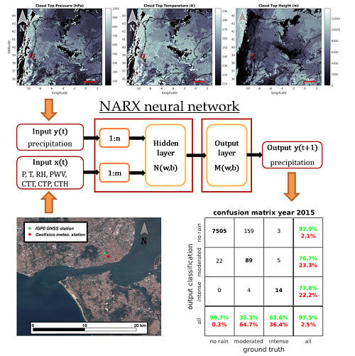
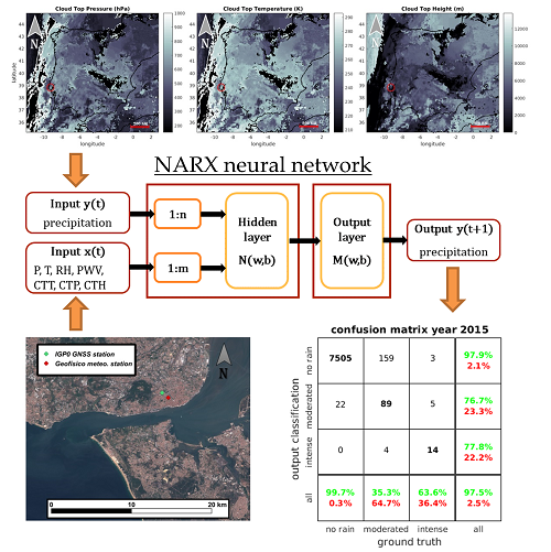
2.1. Neural Network Approach
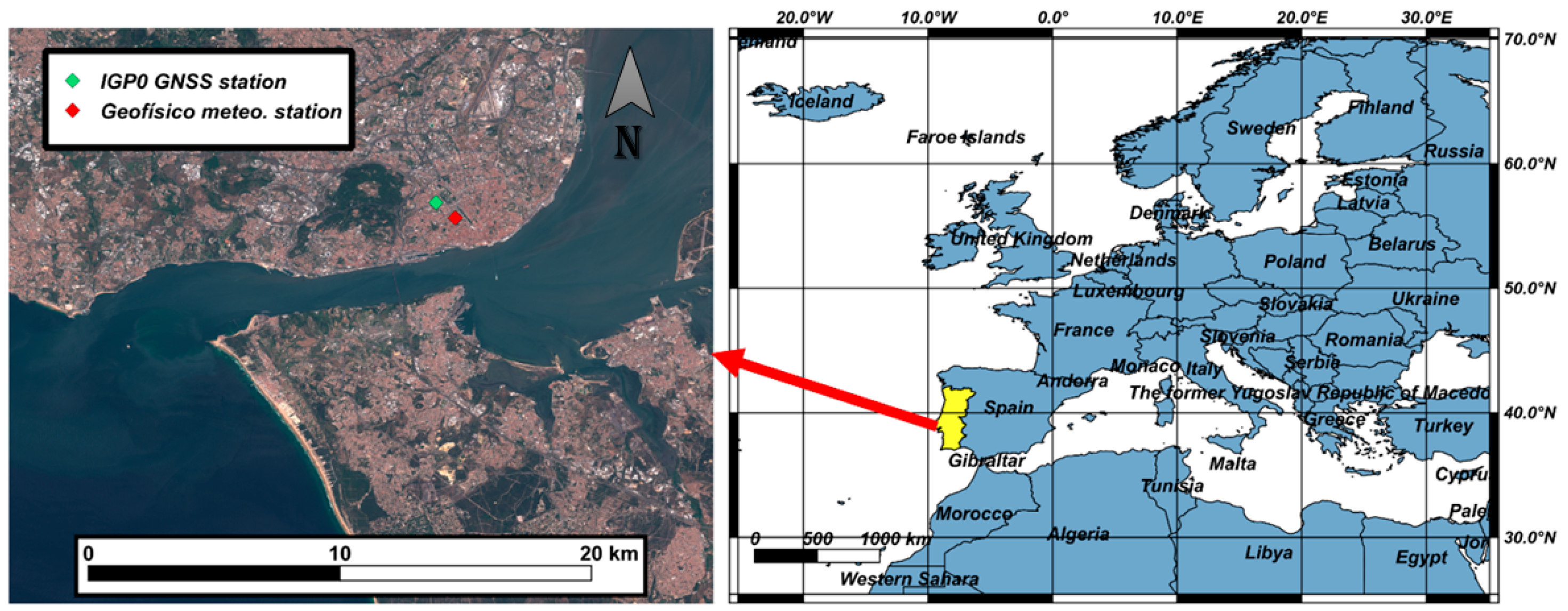
2.2. Study Region
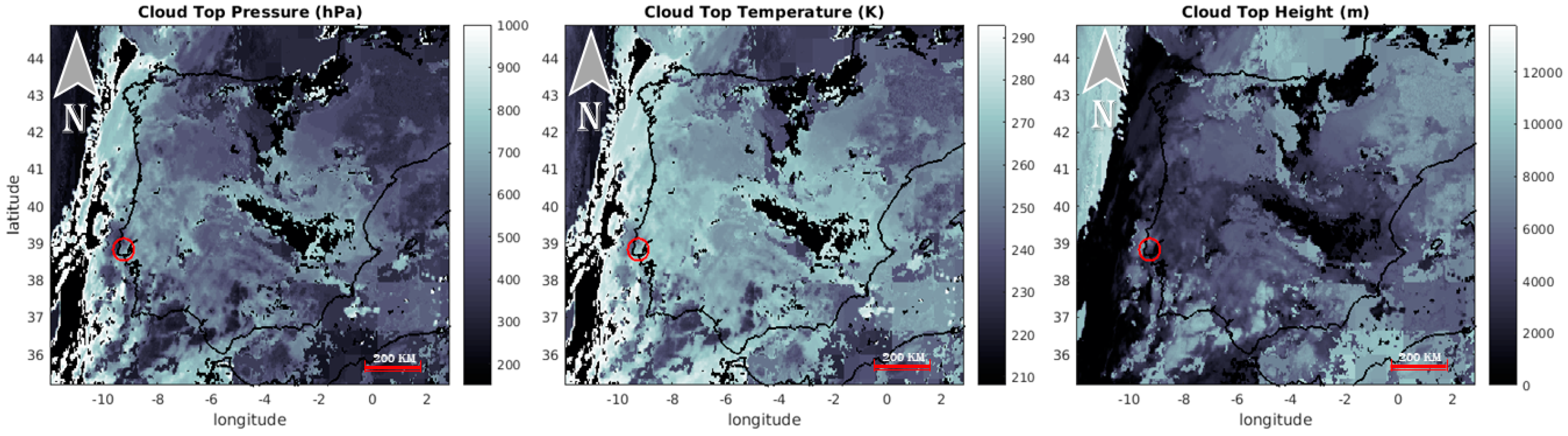
2.3. SEVIRI Data
2.4. GNSS Data Processing
2.5. Data Handling and Integration
3. Results and Discussion
3.1. Neural Network Configuration
3.2. Network Sensitivity to Parameters
3.3. Network Sensitivity to Input Variables
3.4. Network Sensitivity to Data Division
3.5. Best Case with Optimized Parameters
4. Conclusions
Author Contributions
Funding
Acknowledgments
Conflicts of Interest
References
- Yan, X.; Ducrocq, V.; Poli, P.; Hakam, M.; Jaubert, G.; Walpersdorf, A. Impact of GPS zenith delay assimilation on convective-scale prediction of Mediterranean heavy rainfall. J. Geophys. Res. Atmos. 2009, 114. [Google Scholar] [CrossRef] [Green Version]
- Mateus, P.; Miranda, P.M.A.; Nico, G.; Catalão, J.; Pinto, P.; Tomé, R. Assimilating InSAR maps of water vapor to improve heavy rainfall forecasts: A case study with two successive storms. J. Geophys. Res. Atmos. 2018, 123, 3341–3355. [Google Scholar] [CrossRef]
- Brenot, H.; Neméghaire, J.; Delobbe, L.; Clerbaux, N.; De Meutter, P.; Deckmyn, A.; Delcloo, A.; Frappez, L.; Van Roozendael, M. Preliminary signs of the initiation of deep convection by GNSS. Atmos. Chem. Phys. 2013, 13, 5425–5449. [Google Scholar] [CrossRef] [Green Version]
- Mateus, P.; Nico, G.; Catalao, J. Uncertainty Assessment of the Estimated Atmospheric Delay Obtained by a Numerical Weather Model (NMW). IEEE Trans. Geosci. Remote Sens. 2015, 53, 6710–6717. [Google Scholar] [CrossRef]
- Guerova, G.; Jones, J.; Douša, J.; Dick, G.; Haan, S.D.; Pottiaux, E.; Bock, O.; Pacione, R.; Elgered, G.; Vedel, H.; et al. Review of the state of the art and future prospects of the ground-based GNSS meteorology in Europe. Atmos. Meas. Tech. 2016, 9, 5385–5406. [Google Scholar] [CrossRef] [Green Version]
- Suparta, W.; Ali, M. Nowcasting the lightning activity in Peninsular Malaysia using the GPS PWV during the 2009 intermonsoons. Ann. Geophys. 2014, 57, A0217. [Google Scholar] [CrossRef]
- Barindelli, S.; Realini, E.; Venuti, G.; Fermi, A.; Gatti, A. Detection of water vapor time variations associated with heavy rain in northern Italy by geodetic and low-cost GNSS receivers. Earth Planets Space 2018, 70, 28. [Google Scholar] [CrossRef] [Green Version]
- De Haan, S. Assimilation of GNSS ZTD and radar radial velocity for the benefit of very-short-range regional weather forecasts. Q. J. R. Meteorol. Soc. 2013, 139, 2097–2107. [Google Scholar] [CrossRef] [Green Version]
- Benevides, P.; Nico, G.; Catalao, J.; Miranda, P.M.A. Analysis of Galileo and GPS Integration for GNSS Tomography. IEEE Trans. Geosci. Remote Sens. 2017, 55, 1936–1943. [Google Scholar] [CrossRef]
- Dousa, J.; Vaclavovic, P. Real-time zenith tropospheric delays in support of numerical weather prediction applications. Adv. Space Res. 2014, 53, 1347–1358. [Google Scholar] [CrossRef]
- Benevides, P.; Catalao, J.; Miranda, P.M.A. On the inclusion of GPS precipitable water vapour in the nowcasting of rainfall. Nat. Hazards Earth Syst. Sci. 2015, 15, 2605–2616. [Google Scholar] [CrossRef] [Green Version]
- Yao, Y.; Shan, L.; Zhao, Q. Establishing a method of short-term rainfall forecasting based on GNSS-derived PWV and its application. Sci. Rep. 2017, 7, 12465. [Google Scholar] [CrossRef] [Green Version]
- Manandhar, S.; Lee, Y.H.; Meng, Y.S.; Yuan, F.; Ong, J.T. GPS-Derived PWV for Rainfall Nowcasting in Tropical Region. IEEE Trans. Geosci. Remote Sens. 2018, 56, 4835–4844. [Google Scholar] [CrossRef]
- French, M.N.; Krajewski, W.F.; Cuykendall, R.R. Rainfall forecasting in space and time using a neural network. J. Hydrol. 1992, 137, 1–31. [Google Scholar] [CrossRef]
- Hall, T.; Brooks, H.E.; Doswell III, C.A. Precipitation forecasting using a neural network. Weather Forecast. 1999, 14, 338–345. [Google Scholar] [CrossRef]
- Ramirez, M.C.V.; de Campos Velho, H.F.; Ferreira, N.J. Artificial neural network technique for rainfall forecasting applied to the Sao Paulo region. J. Hydrol. 2005, 301, 146–162. [Google Scholar] [CrossRef]
- Rivolta, G.; Marzano, F.S.; Coppola, E.; Verdecchia, M. Artificial neural-network technique for precipitation nowcasting from satellite imagery. Adv. Geosci. 2006, 7, 97–103. [Google Scholar] [CrossRef] [Green Version]
- Hung, N.Q.; Babel, M.S.; Weesakul, S.; Tripathi, N.K. An artificial neural network model for rainfall forecasting in Bangkok, Thailand. Hydrol. Earth Syst. Sci. 2009, 13, 1413–1425. [Google Scholar] [CrossRef] [Green Version]
- Wu, C.L.; Chau, K.W.; Fan, C. Prediction of rainfall time series using modular artificial neural networks coupled with data-preprocessing techniques. J. Hydrol. 2010, 389, 146–167. [Google Scholar] [CrossRef] [Green Version]
- Shi, X.; Chen, Z.; Wang, H.; Yeung, D.Y.; Wong, W.K.; Woo, W.C. Convolutional LSTM network: A machine learning approach for precipitation nowcasting. In Proceedings of the Advances in Neural Information Processing Systems, Montreal, QC, Canada, 7–12 December 2015; pp. 802–810. [Google Scholar]
- Suparta, W.; Alhasa, K.M. Modeling of zenith path delay over Antarctica using an adaptive neuro fuzzy inference system technique. Expert Syst. Appl. 2015, 42, 1050–1064. [Google Scholar] [CrossRef]
- Ding, M. A neural network model for predicting weighted mean temperature. J. Geod. 2018, 92, 1187–1198. [Google Scholar] [CrossRef]
- Suparta, W.; Alhasa, K.M. Modeling of precipitable water vapor using an adaptive neuro-fuzzy inference system in the absence of the GPS network. J. Appl. Meteorol. Climatol. 2016, 55, 2283–2300. [Google Scholar] [CrossRef]
- Rahimi, Z.; Shafri, H.Z.M.; Norman, M. A GNSS-based weather forecasting approach using Nonlinear Auto Regressive Approach with Exogenous Input (NARX). J. Atmos. Sol.-Terr. Phys. 2018, 178, 74–84. [Google Scholar] [CrossRef]
- Lin, T.; Horne, B.G.; Tino, P.; Giles, C.L. Learning long-term dependencies in NARX recurrent neural networks. IEEE Trans. Neural Netw. 1996, 7, 1329–1338. [Google Scholar] [CrossRef] [Green Version]
- Finkensieper, S.; Meirink, J.F.; van Zadelhoff, G.J.; Hanschmann, T.; Benas, N.; Stengel, M.; Fuchs, P.; Hollmann, R.; Werscheck, M. CLAAS-2: CM SAF CLoud Property dAtAset Using SEVIRI. Available online: https://bit.ly/2GrdHU2 (accessed on 22 April 2019).
- Herring, T.; King, R.W.; McClusky, S.C. GAMIT Reference Manual—GPS Analysis at MIT—Release 10.4; Department of Earth, Atmospheric and Planetary Sciences, MIT: Cambridge, MA, USA, 2010. [Google Scholar]
- Benevides, P.; Catalao, J.; Nico, G.; Miranda, P.M.A. 4D wet refractivity estimation in the atmosphere using GNSS tomography initialized by radiosonde and AIRS measurements: Results from a 1-week intensive campaign. GPS Solut. 2018, 22, 91. [Google Scholar] [CrossRef]
- Bevis, M.; Businger, S.; Herring, T.; Rocken, C.; Anthes, R.A.; Ware, R.H. GPS meteorology: Remote sensing of the atmospheric water vapor using the Global Positioning System. J. Geophys. Res. 1992, 97, 15787–15801. [Google Scholar] [CrossRef]
- Mateus, P.; Nico, G.; Catalão, J. Maps of PWV temporal changes by SAR interferometry: A study on the properties of atmosphere’s temperature profiles. IEEE Geosci. Remote Sens. Lett. 2014, 11, 2065–2069. [Google Scholar] [CrossRef]
- Yaghini, M.; Khoshraftar, M.M.; Fallahi, M. A hybrid algorithm for artificial neural network training. Eng. Appl. Artif. Intell. 2013, 26, 293–301. [Google Scholar] [CrossRef]


| Variable Name | Source | Acronym | Units | Function |
|---|---|---|---|---|
| Hourly precipitation | Meteorological station | Rain | mm/h | Input/Output |
| Precipitable water vapor | GNSS station | PWV | mm | Input |
| Pressure | Meteorological station | P | hPa | Input |
| Temperature | Meteorological station | T | °C | Input |
| Relative Humidity | Meteorological station | RH | % | Input |
| Cloud Top Temperature | Remote sensing | CTT | K | Input |
| Cloud Top Pressure | Remote sensing | CTP | hPa | Input |
| Cloud Top Height | Remote sensing | CTH | m | Input |
| Variable Name | Values |
|---|---|
| # Hidden layers | 1 |
| # Neurons | 10 |
| # Delays | 6 |
| Training function | Levenberg-Marquardt |
| Data weighting | Random |
| Performance evaluation | Mean square error |
| Data division | Step 1: (66%/10%/24%)—4 years |
| (training/validation/testing) | Step 2: (0%/0%/100%)—1 year |
| # Total input variables | 8 |
| # Output variables | 1 |
| # Number of samples | 41427 |
| Precipitation Class | Rain Classification (mm/h) | Number of Samples (hour) | ||
|---|---|---|---|---|
| 4 Years | 1 Year | Total | ||
| No rain | 0 | 31284 | 7527 | 38811 |
| Moderated rain | > 0 < 5 | 2184 | 252 | 2436 |
| Intense rain | >= 5 | 159 | 22 | 181 |
| Neural Network with 7 Variables (GNSS+Meteo+Sat.) | Intense Rain Class | Test Dataset | ||
|---|---|---|---|---|
| Good Classification | False Positives | Net.RMS | Correlation Coefficient | |
| 10 N, 6 ID 6 FD, Levenberg-Marquardt | 59.1% | 29.6% | 0.467 | 0.824 |
| 10 N, 8 ID 8 FD, Levenberg-Marquardt | 59.1% | 28.7% | 0.470 | 0.821 |
| 2 N, 6 ID 6 FD, Levenberg-Marquardt | 59.1% | 26.4% | 0.472 | 0.818 |
| 10 N, 6 ID 6 FD, Bayesian regularization | 59.1% | 26.0% | 0.489 | 0.803 |
| Neural Network with 7 Variables (GNSS+Meteo+Satellite) | # var. | Intense Rain Class | Test Dataset | ||
|---|---|---|---|---|---|
| Good Classification | False Positives | Net.RMS | Correlation Coefficient | ||
| GNSS + Meteo. + Satellite (PWV,P,T,RH,CTT,CTP,CTH) | 7 | 59.1% | 26.5% | 0.475 | 0.819 |
| GNSS + Meteo. (PWV,P,T,RH) | 4 | 58.9% | 27.1% | 0.471 | 0.821 |
| GNSS (PWV) | 1 | 59.3% | 22.6% | 0.471 | 0.817 |
| Precipitation (NAR model) | 1 | 58.2% | 22.7% | 0.474 | 0.815 |
| Neural Network with 7 Variables (GNSS+Meteo+Satellite) | #Intense Rain | Intense Rain Class | Test Dataset | ||
|---|---|---|---|---|---|
| Good Classification | False Positives | Net.RMS | Correlation Coefficient | ||
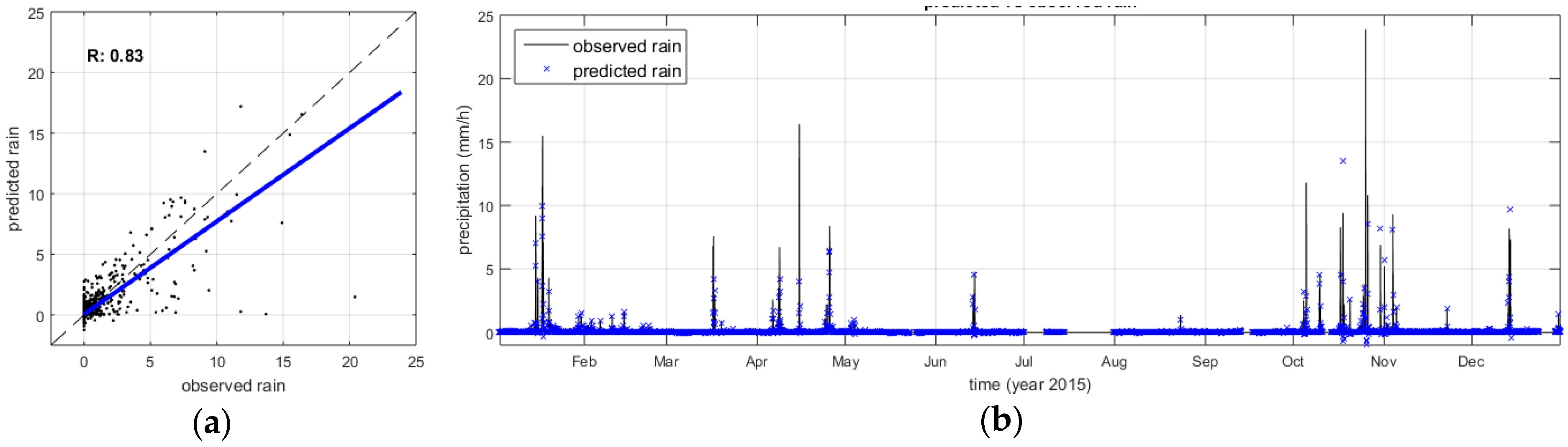
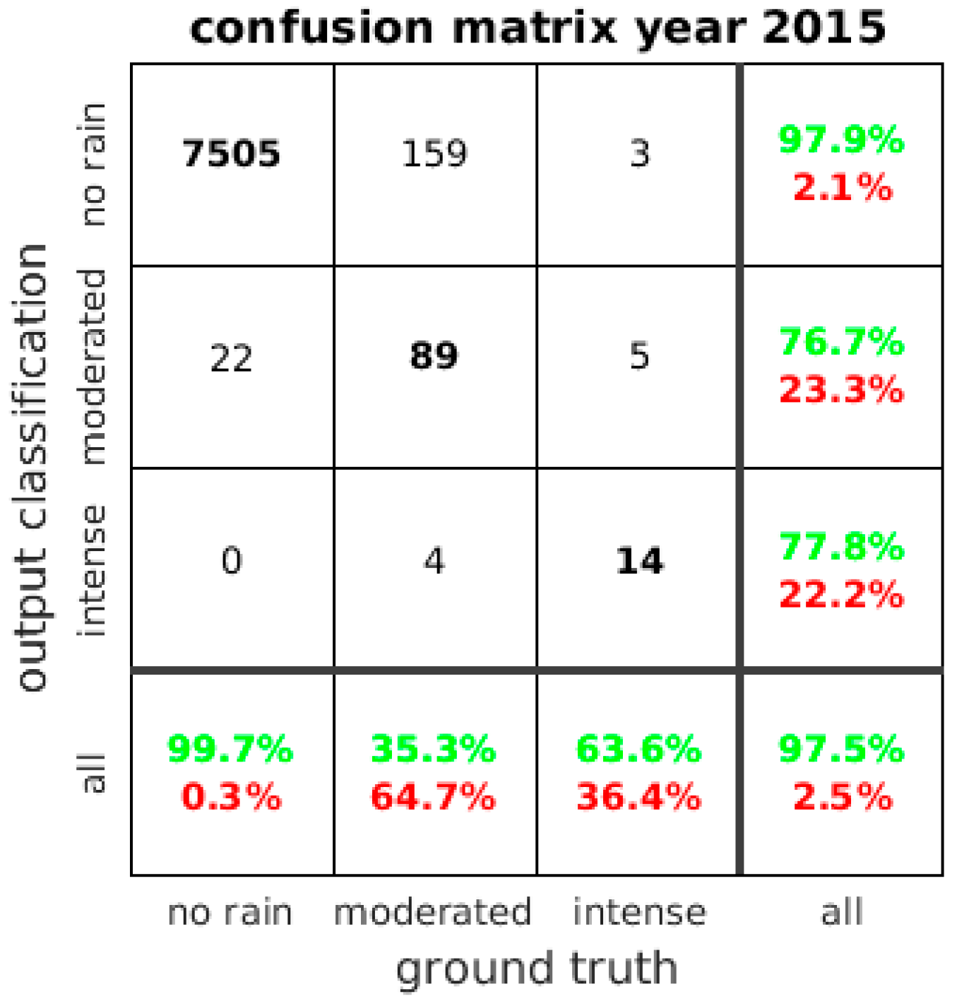
| 2015 test dataset | 22 | 63.6% | 22.2% | 0.464 | 0.826 |
| 2011 test dataset | 57 | 63.3% | 35.6% | 0.875 | 0.828 |
| 2012 test dataset | 32 | 71.9% | 23.3% | 0.589 | 0.875 |
| 2013 test dataset | 37 | 66.0% | 20.5% | 0.807 | 0.820 |
| 2014 test dataset | 41 | 64.3% | 30.8% | 0.726 | 0.831 |
© 2019 by the authors. Licensee MDPI, Basel, Switzerland. This article is an open access article distributed under the terms and conditions of the Creative Commons Attribution (CC BY) license (http://creativecommons.org/licenses/by/4.0/).
Share and Cite
Benevides, P.; Catalao, J.; Nico, G. Neural Network Approach to Forecast Hourly Intense Rainfall Using GNSS Precipitable Water Vapor and Meteorological Sensors. Remote Sens. 2019, 11, 966. https://0-doi-org.brum.beds.ac.uk/10.3390/rs11080966
Benevides P, Catalao J, Nico G. Neural Network Approach to Forecast Hourly Intense Rainfall Using GNSS Precipitable Water Vapor and Meteorological Sensors. Remote Sensing. 2019; 11(8):966. https://0-doi-org.brum.beds.ac.uk/10.3390/rs11080966
Chicago/Turabian StyleBenevides, Pedro, Joao Catalao, and Giovanni Nico. 2019. "Neural Network Approach to Forecast Hourly Intense Rainfall Using GNSS Precipitable Water Vapor and Meteorological Sensors" Remote Sensing 11, no. 8: 966. https://0-doi-org.brum.beds.ac.uk/10.3390/rs11080966