SPA-Based Methods for the Quantitative Estimation of the Soil Salt Content in Saline-Alkali Land from Field Spectroscopy Data: A Case Study from the Yellow River Irrigation Regions


Abstract
:1. Introduction
2. Materials
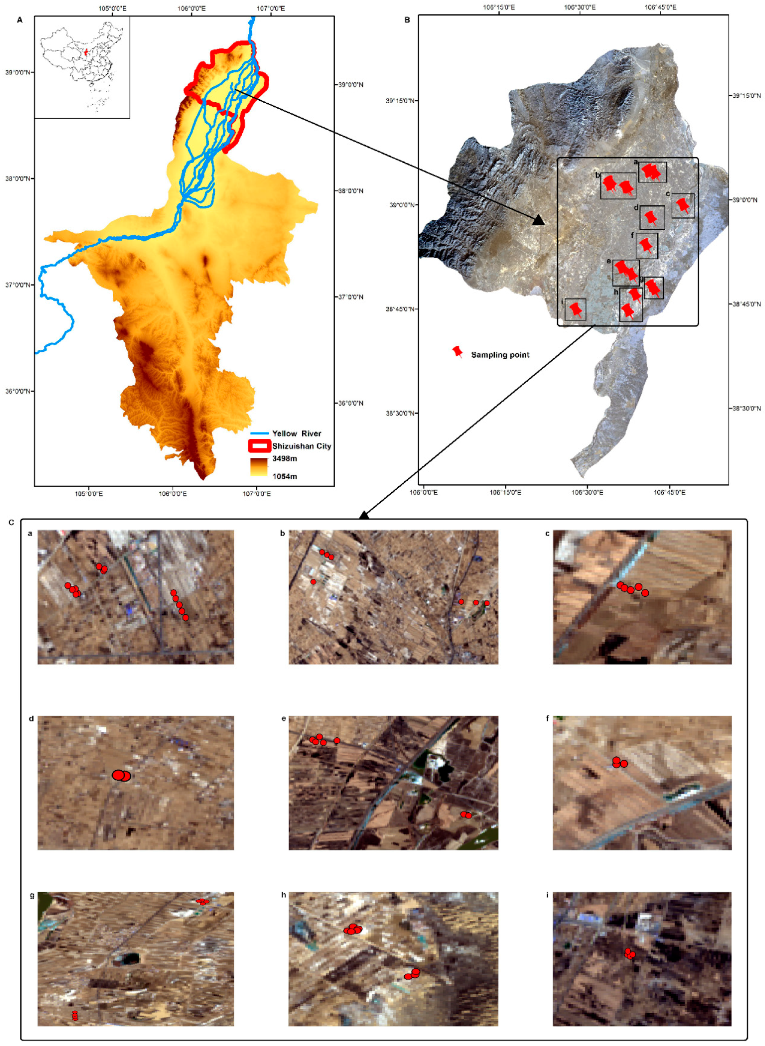
2.1. Study Area
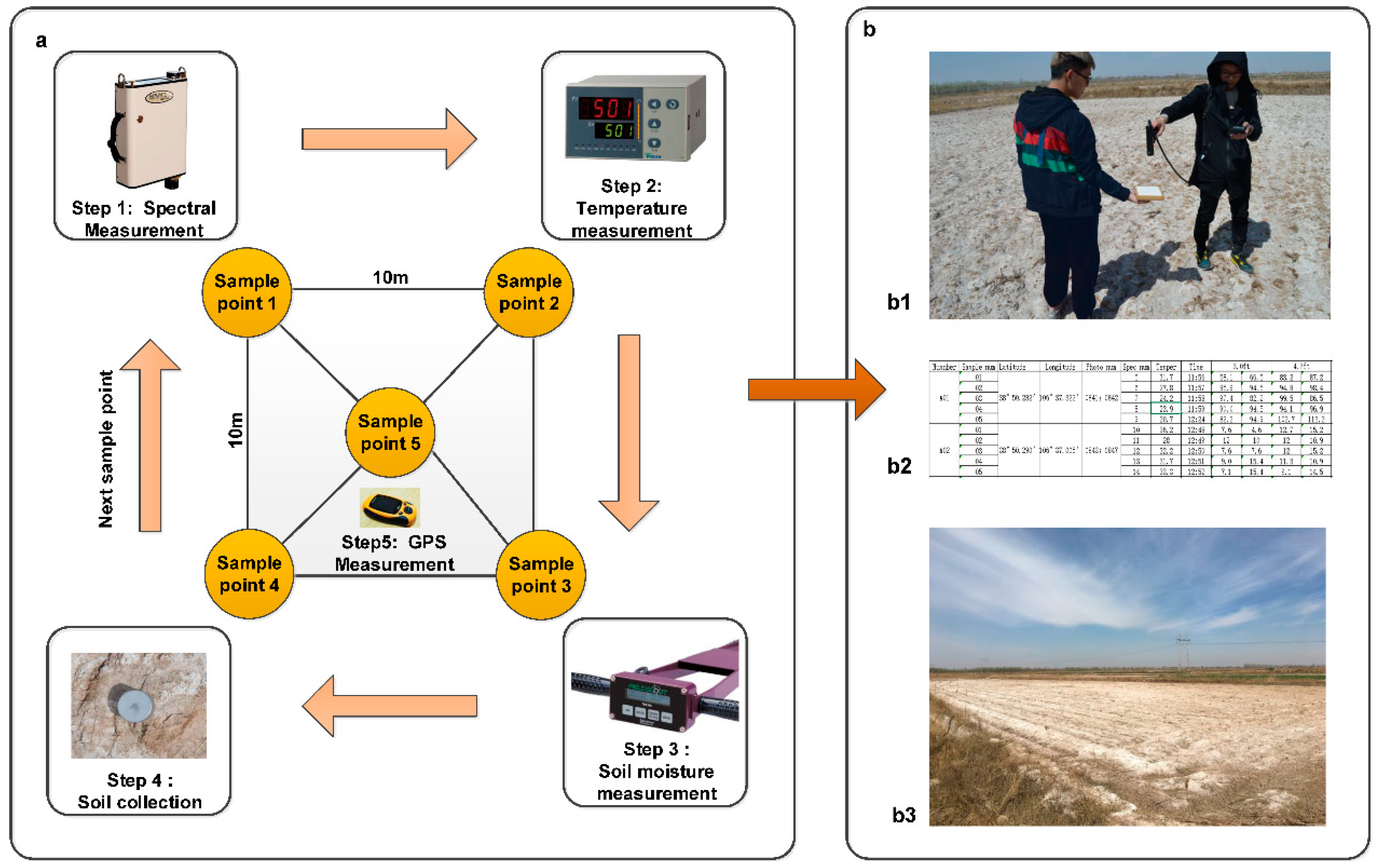
2.2. Sampling and Spectral Measurements
3. Methods
3.1. Soil Parameters Analysis Method
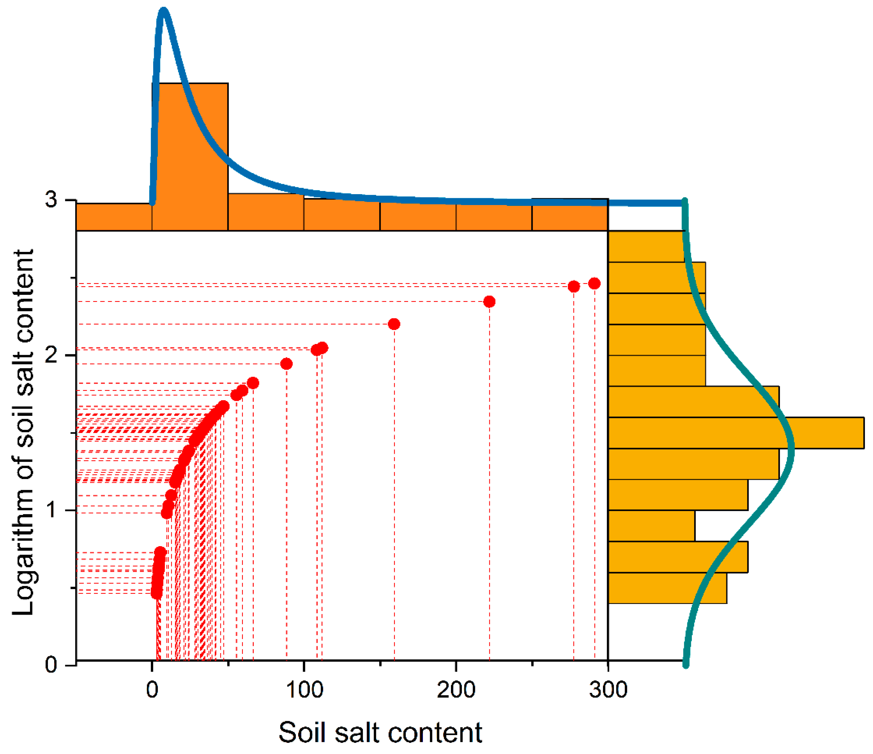
3.2. Processing Transformation
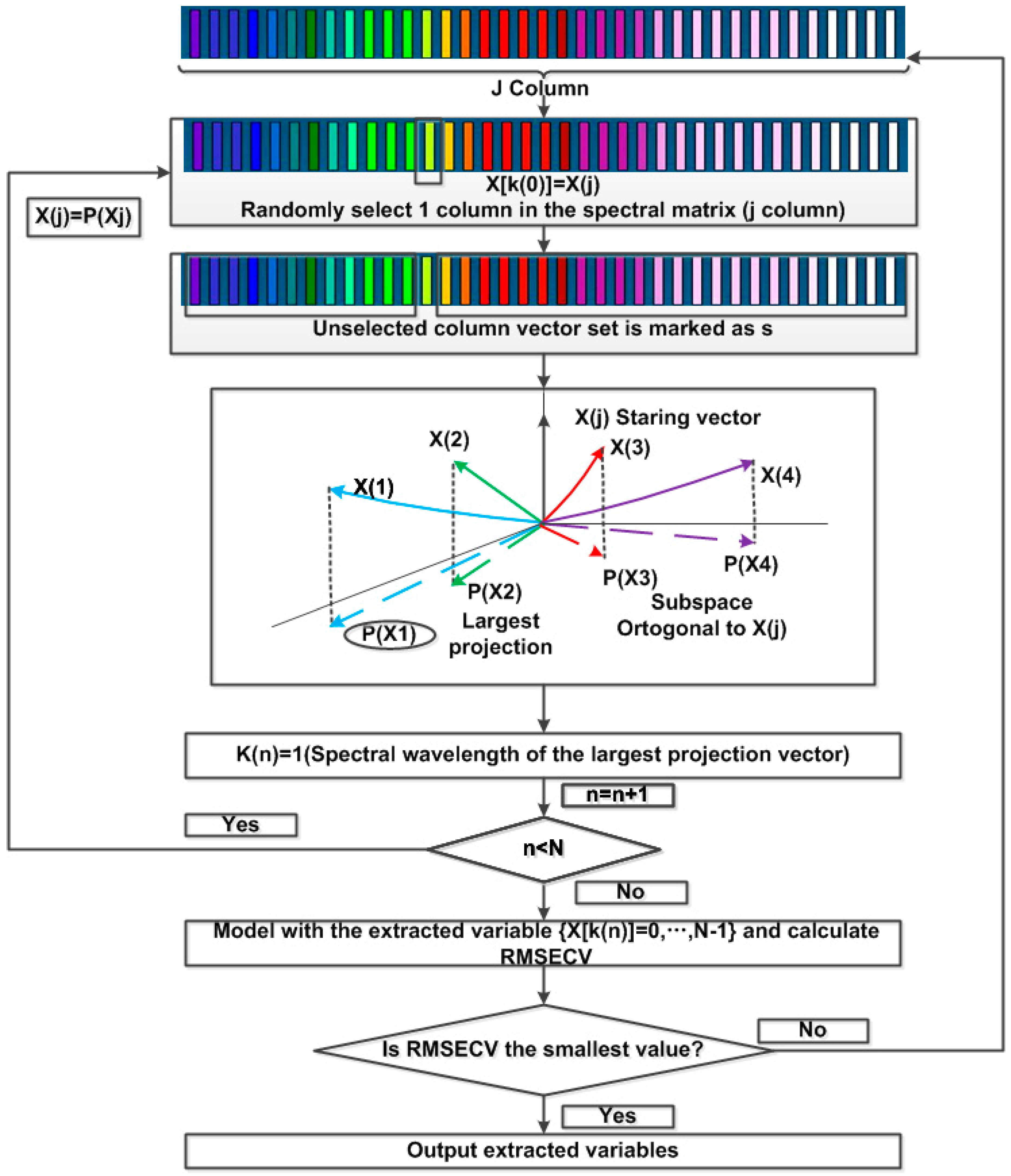
3.3. Successive Projections Algorithm
3.4. Partial Least Squares Regression (PLSR)
3.5. Prediction Accuracy
4. Results
4.1. Salinity Parameters
4.2. Characteristic Analysis of the Varying Spectra
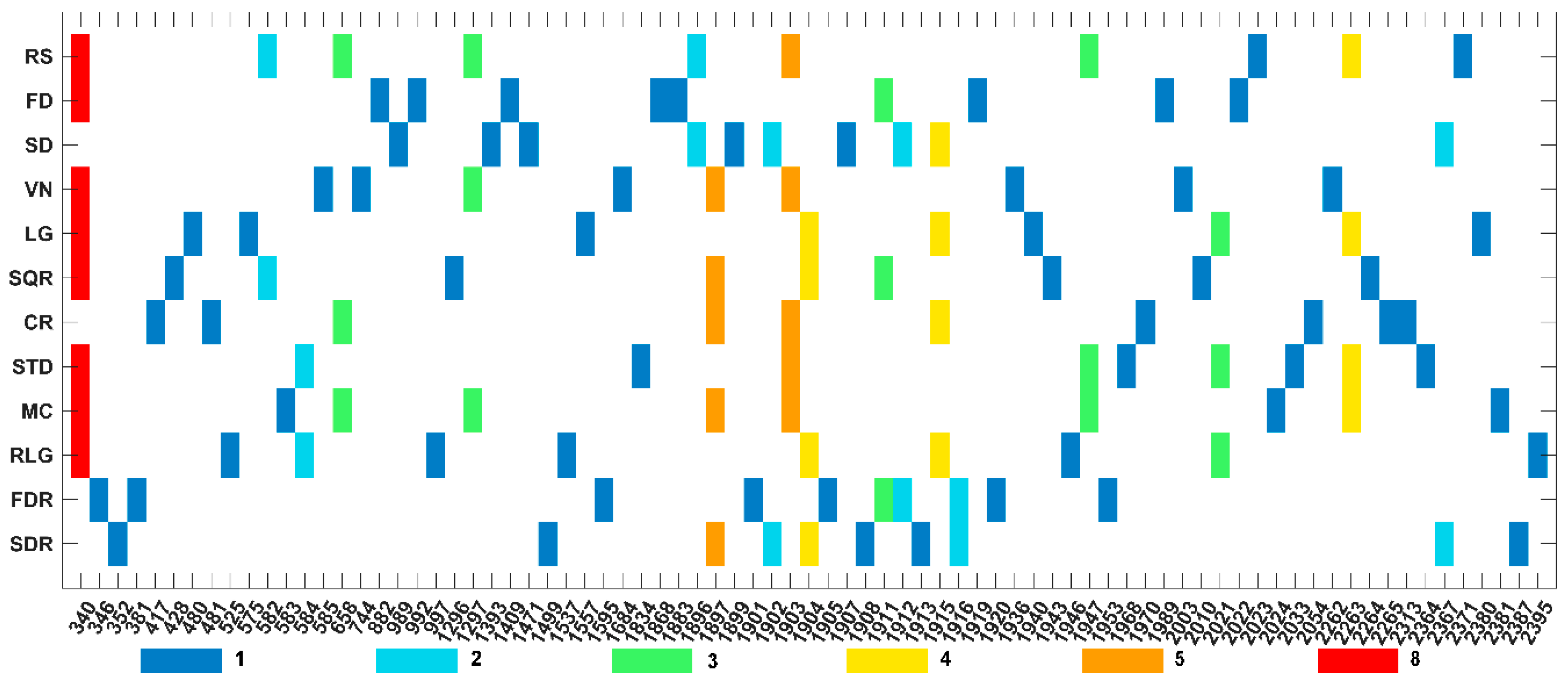
4.3. Feature Band Selected by the SPA Method
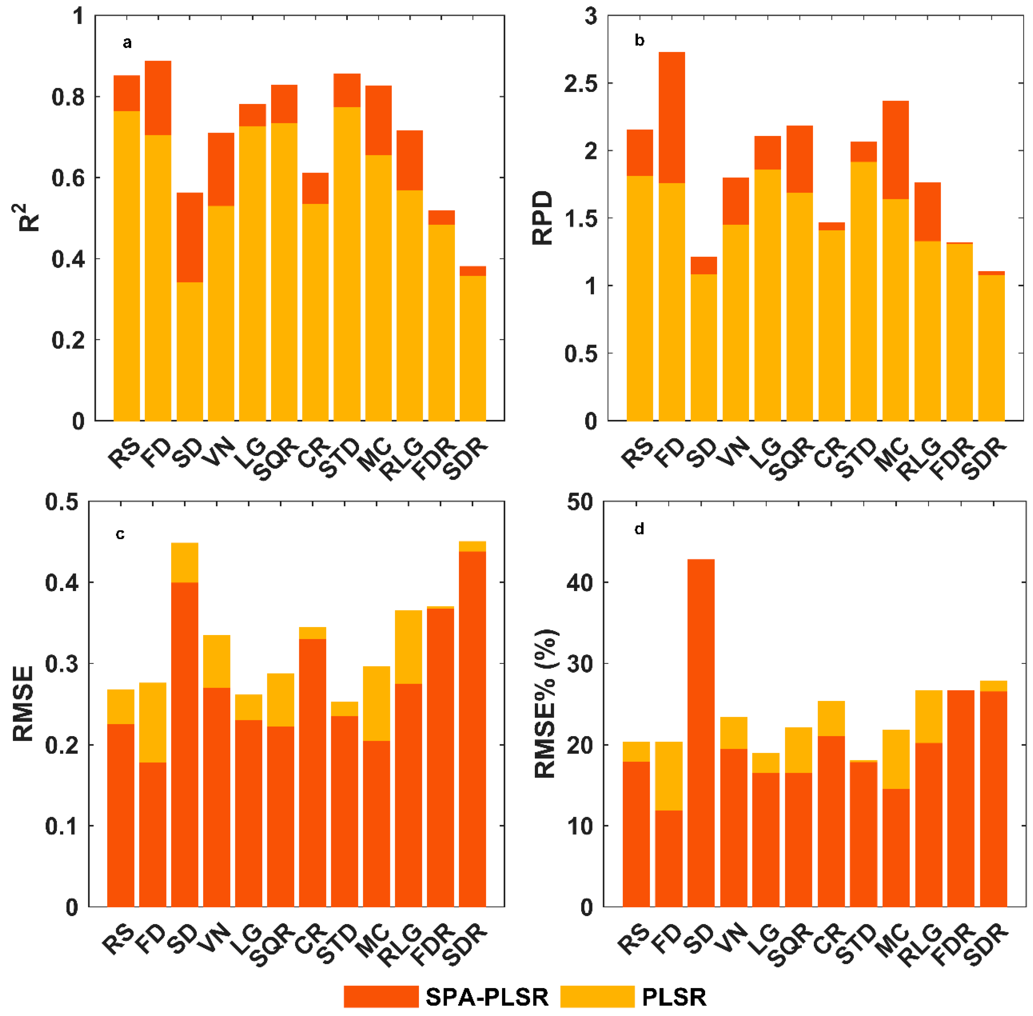
4.4. Performance of SPA–PLSR
5. Discussion
5.1. Feature Bands
5.2. The Effect of the SPA Method
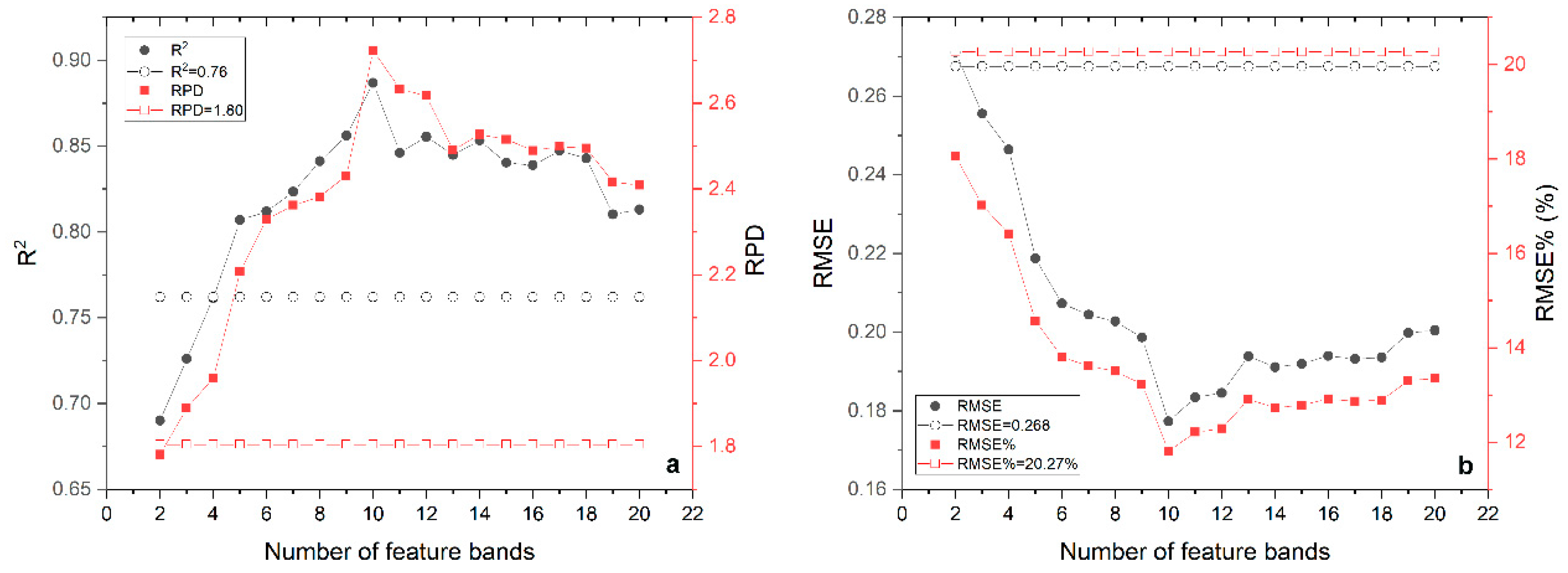
5.3. The Effect of Selecting the Number of Feature Bands on the Model
5.4. The Availability of the Model
6. Conclusions
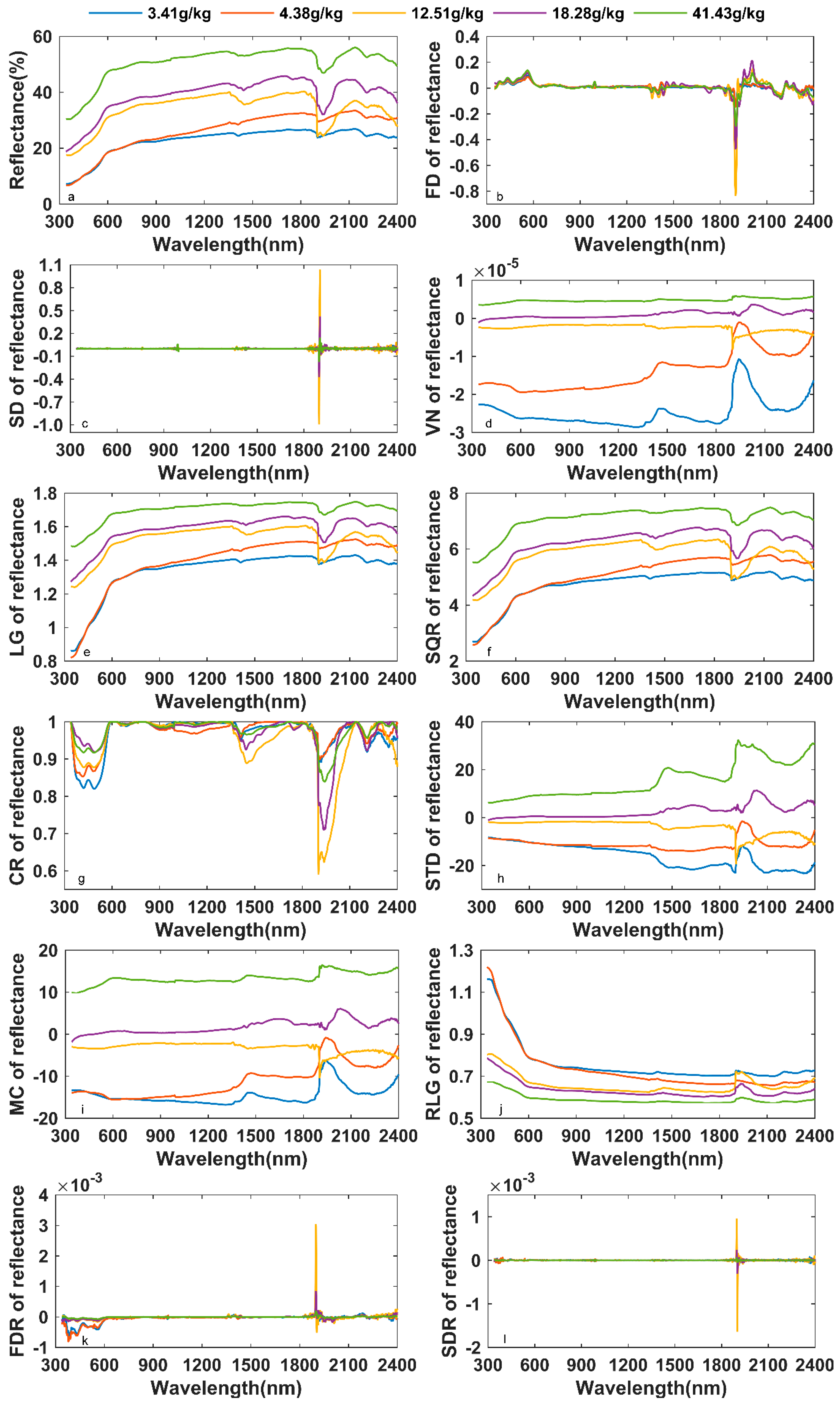
- In addition to SD, FDR, and SDR, the other nine kinds of spectra could show different changes in soil salt content to varying degrees.
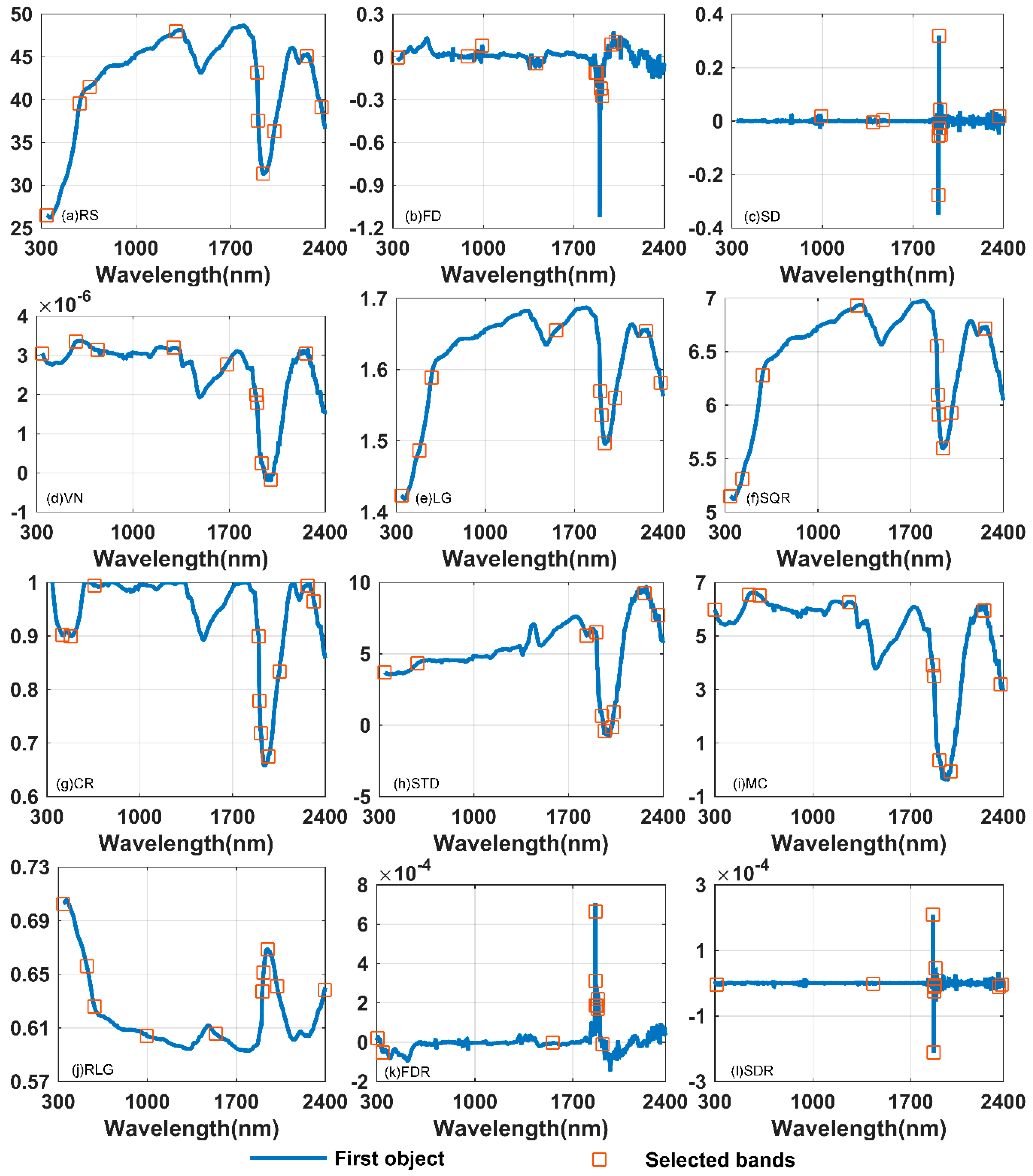
- Sensitive bands for soil salt content were 340–481 nm, 525–744 nm, 882–997 nm, 1296–1393 nm, 1409–1684 nm, 1834–1899 nm, 1901–2054 nm, 2262–2395 nm. The most sensitive bands were concentrated at 525–744 nm, 1834–1899 nm, and 1901–2054 nm.
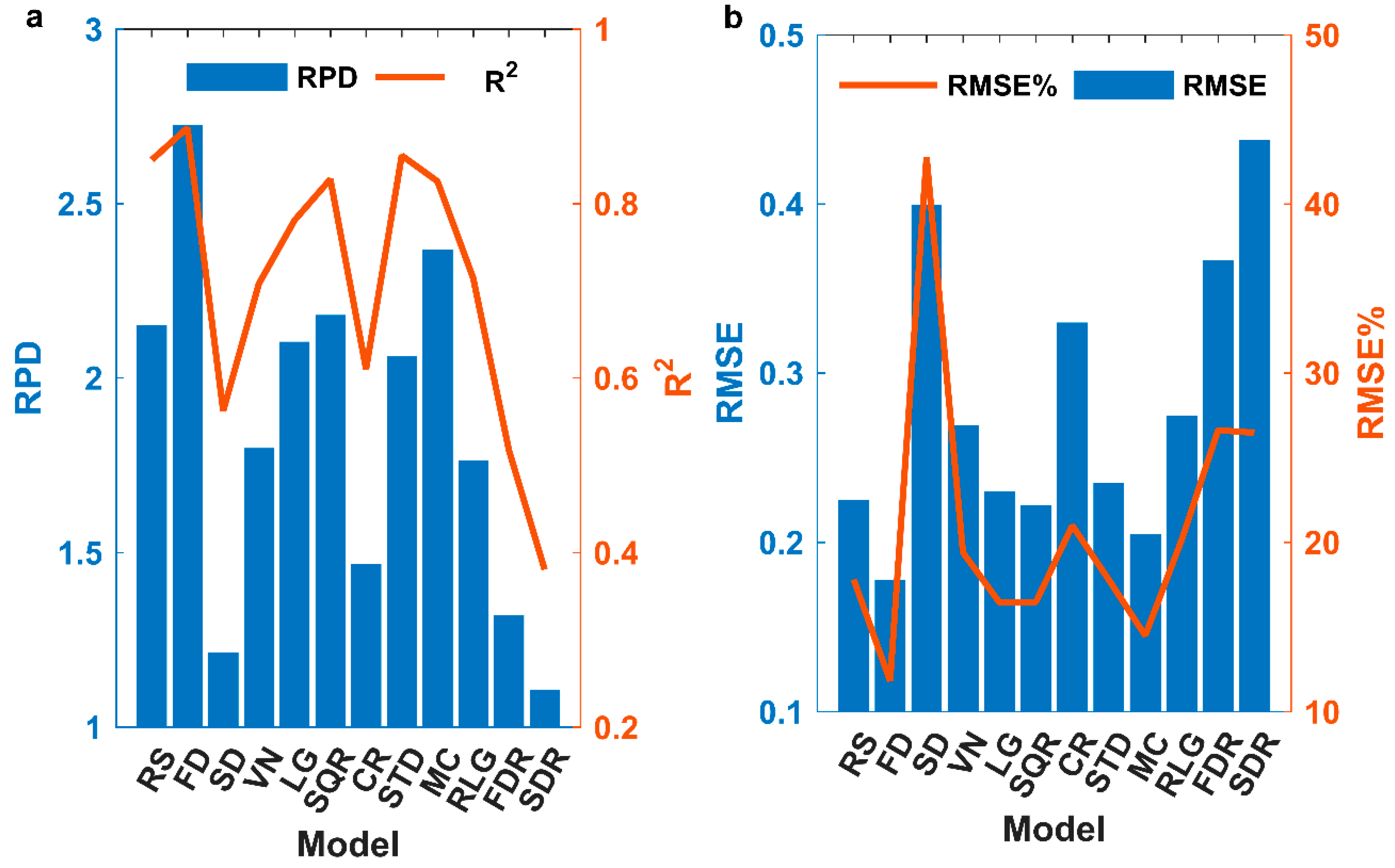
- Modeling PLSR with feature bands selected by SPA could effectively improve the and RPD of the model.
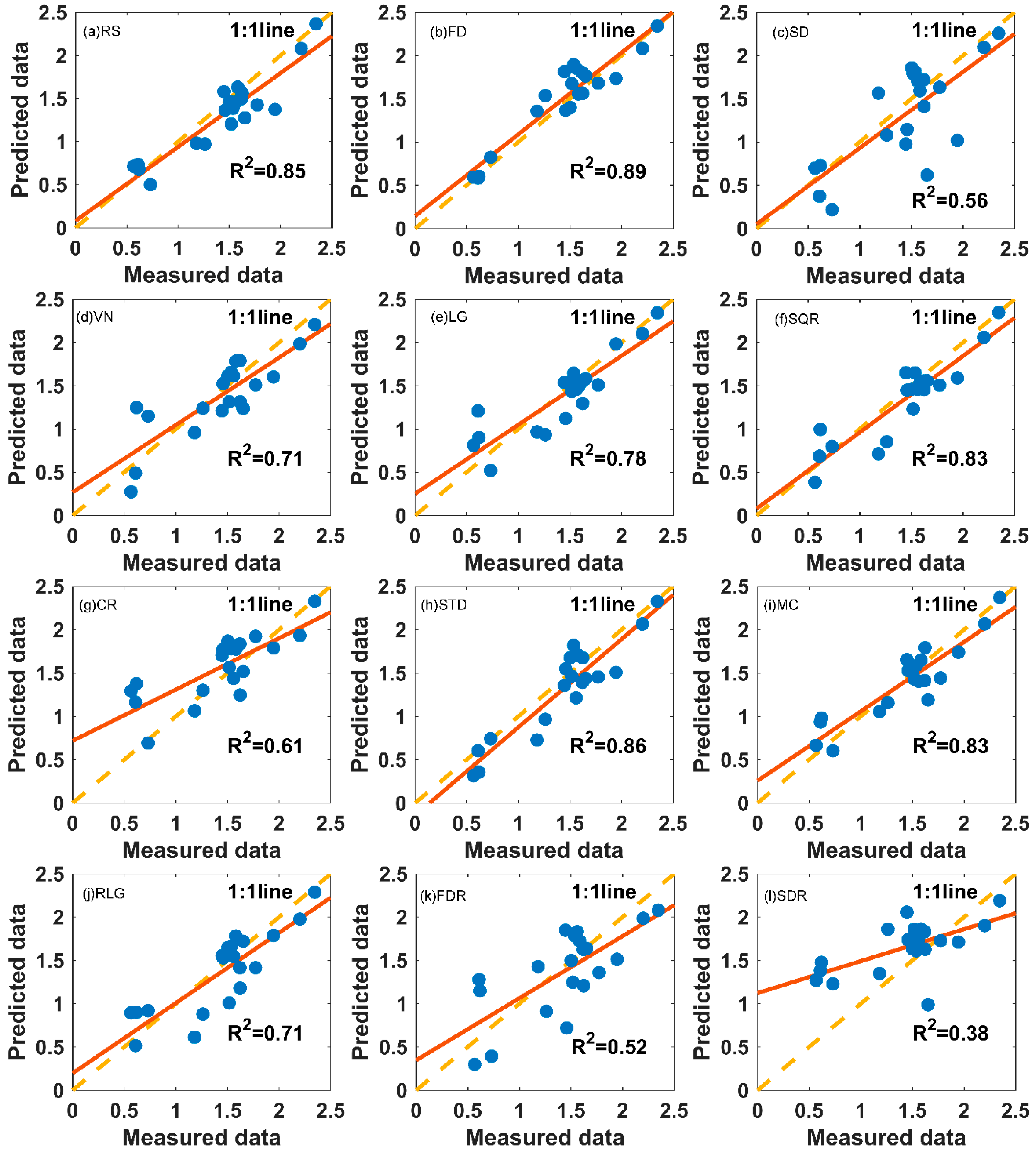
- The FD–SPA–PLSR model had the best estimation results. This model could estimate the soil salt content when the number of bands was greater than 5. The best estimation result could be obtained when the number of bands was 10. Compared with the RS–PLSR model, R2 was increased from 0.76 to 0.89, the RPD was increased from 1.80 to 2.72, the RMSE was decreased from 0.268 to 0.177, and the RMSE% was decreased from 20.27% to 11.81%.
Author Contributions
Funding
Conflicts of Interest
References
- Zhang, D. Application Research of Fractional Derivative in the Remote Sensing Monitoring of Soil Salinization. Ph.D. Thesis, Xinjiang University, Urumqi, China, 2017. [Google Scholar]
- Li, T. Study on Typical Saline Region by Remote Sensing Monitoring in the Yellow River Delta. Master’s Thesis, China University of Petroleum (East China), Qingdao, China, 2015. [Google Scholar]
- Zhang, T. Evaluate and Analyze land Salinization Pattern, Process and Ecological Effects in the Yellow River Delta: Using Remote Sensing and Ecological Models. Ph.D. Thesis, Fudan University, Shanghai, China, 2011. [Google Scholar]
- Hou, C. Research on Remote Sensing Monitoring in the Typical Salt-Affected Zone of the Yellow River Delta Based on BP Neural Net. Master’s Thesis, China University of Petroleum (East China), Qingdao, China, 2010. [Google Scholar]
- Bakker, D.M.; Hamilton, G.J.; Hetherington, R.; Spann, C. Salinity dynamics and the potential for improvement of waterlogged and saline land in a Mediterranean climate using permanent raised beds. Soil Tillage Res. 2010, 110, 8–24. [Google Scholar] [CrossRef]
- Cécile, G.; Philippe, L.; Guillaume, C. Regional predictions of eight common soil properties and their spatial structures from hyperspectral Vis–NIR data. Geoderma 2012, 189–190, 176–185. [Google Scholar]
- Hu, J.; Peng, J.; Zhou, Y.; Xu, D.Y.; Zhao, R.Y.; Jiang, Q.S.; Fu, T.T.; Wang, F.; Shi, Z. Quantitative Estimation of Soil Salinity Using UAV-Borne Hyperspectral and Satellite Multispectral Images. Remote Sens. 2019, 11, 736. [Google Scholar] [CrossRef]
- Xu, C.; Zeng, W.; Huang, J.; Wu, J.; Van Leeuwen, W.J. Prediction of Soil Moisture Content and Soil Salt Concentration from Hyperspectral Laboratory and Field Data. Remote Sens. 2016, 8, 42. [Google Scholar] [CrossRef]
- Sadro, S.; Gastilbuhl, M.; Melack, J.M. Characterizing patterns of plant distribution in a southern California salt marsh using remotely sensed topographic and hyperspectral data and local tidal fluctuations. Remote Sens. Environ. 2007, 110, 226–239. [Google Scholar] [CrossRef]
- Sytar, O.; Brestic, M.; Zivcak, M.; Olsovska, K.; Kovar, M.; Shao, H.; He, X. Applying hyperspectral imaging to explore natural plant diversity towards improving salt stress tolerance. Sci. Total Environ. 2017, 578, 90–99. [Google Scholar] [CrossRef] [PubMed] [Green Version]
- Nawar, S.; Buddenbaum, H.; Hill, J. Estimation of soil salinity using three quantitative methods based on visible and near-infrared reflectance spectroscopy: A case study from Egypt. Arab. J. Geosci. 2015, 8, 5127–5140. [Google Scholar] [CrossRef]
- Scudiero, E.; Skaggs, T.H.; Corwin, D.L. Regional-scale soil salinity assessment using Landsat ETM+ canopy reflectance. Remote Sens. Environ. 2015, 169, 335–343. [Google Scholar] [CrossRef]
- Bouaziz, M.; Matschullat, J.; Gloaguen, R. Improved remote sensing detection of soil salinity from a semi-arid climate in Northeast Brazil. C. R. Geosci. 2011, 343, 795–803. [Google Scholar] [CrossRef]
- Lobell, D.B.; Lesch, S.M.; Corwin, D.L.; Ulmer, M.G.; Anderson, K.A.; Potts, D.J.; Doolittle, J.A.; Matos, M.R.; Baltes, M.J. Regional-scale Assessment of Soil Salinity in the Red River Valley Using Multi-year MODIS EVI and NDVI. J. Environ. Qual. 2010, 39, 35–41. [Google Scholar] [CrossRef]
- Yan, L.I.; Shi, Z.; Cifang, W.U.; Hongyi, L.I.; Feng, L.I. Improved Prediction and Reduction of Sampling Density for Soil Salinity by Different Geostatistical Methods. Agric. Sci. China 2007, 6, 832–841. [Google Scholar]
- Dehaan, R.L.; Taylor, G.R. Field-derived spectra of salinized soils and vegetation as indicators of irrigation-induced soil salinization. Remote Sens. Environ. 2002, 80, 406–417. [Google Scholar] [CrossRef]
- Mashimbye, Z.E.; Cho, M.A.; Nell, J.P.; De Clercq, W.P.; Van Niekerk, A.; Turner, D.P. Model-Based Integrated Methods for Quantitative Estimation of Soil Salinity from Hyperspectral Remote Sensing Data: A Case Study of Selected South African Soils. Pedosphere 2012, 22, 640–649. [Google Scholar] [CrossRef]
- Peng, J.; Wang, J.Q.; Xiang, H.Y.; Teng, H.F.; Liu, W.Y.; Chi, C.M.; Niu, J.L.; Guo, j.; Shi, Z. Comparative Study on Hyperspectral Inversion Accuracy of Soil Salt Content and Electrical Conductivity. Spectrosc. Spectr. Anal. 2014, 34, 510. [Google Scholar]
- Zhang, T.; Zeng, S.; Gao, Y.; Ouyang, Z.; Li, B.; Fang, C.; Zhao, B. Using hyperspectral vegetation indices as a proxy to monitor soil salinity. Ecol. Indic. 2011, 11, 1552–1562. [Google Scholar] [CrossRef]
- Farifteh, J.; Der Meer, F.D.; Atzberger, C.; Carranza, E.J. Quantitative analysis of salt-affected soil reflectance spectra: A comparison of two adaptive methods (PLSR and ANN). Remote Sens. Environ. 2007, 110, 59–78. [Google Scholar] [CrossRef]
- Wang, J.; Qin, L.; Wu, G. Application of Successive Projections Algorithm in Quantitative Analysis of Winter Wheat Hyper-spectral Variables. Electron. R D 2011, 38, 13–15. [Google Scholar]
- Cheng, Z.; Zhang, L.Q.; Liu, H.Y.; Zhu, A.S. Successive projections algorithm and its application to selecting the wheat near-infrared spectral variables. Spectrosc. Spectr. Anal. 2010, 30, 949. [Google Scholar]
- Kumar, S.; Gautam, G. Hyperspectral remote sensing data derived spectral indices in characterizing salt-affected soils: A case study of Indo-Gangetic plains of India. Environ. Earth Sci. 2015, 73, 3299–3308. [Google Scholar] [CrossRef]
- Allbed, A.; Kumar, L.; Aldakheel, Y.Y. Assessing soil salinity using soil salinity and vegetation indices derived from IKONOS high-spatial resolution imageries: Applications in a date palm dominated region. Geoderma 2014, 230–231, 1–8. [Google Scholar] [CrossRef]
- De Araujo, M.C.; Saldanha, T.C.; Galvao, R.K.; Yoneyama, T.; Chame, H.C.; Visani, V. The successive projections algorithm for variable selection in spectroscopic multicomponent analysis. Chemom. Intell. Lab. Syst. 2001, 57, 65–73. [Google Scholar] [CrossRef]
- Inácio, M.R.C.; de Moura, M.d.V.; de Lima, K.M.G. Classification and determination of total protein in milk powder using near infrared reflectance spectrometry and the successive projections algorithm for variable selection. Vib. Spectrosc. 2011, 57, 342–345. [Google Scholar] [CrossRef]
- Goudarzi, N.; Goodarzi, M. Application of successive projections algorithm (SPA) as a variable selection in a QSPR study to predict the octanol/water partition coefficients (Kow) of some halogenated organic compounds. Anal. Methods 2010, 2, 758–764. [Google Scholar] [CrossRef]
- Liu, F.; He, Y. Application of successive projections algorithm for variable selection to determine organic acids of plum vinegar. Food Chem. 2009, 115, 1430–1436. [Google Scholar] [CrossRef]
- Tang, R.; Chen, X.; Li, C. Detection of Nitrogen Content in Rubber Leaves Using Near-Infrared (NIR) Spectroscopy with Correlation-Based Successive Projections Algorithm (SPA). Appl. Spectrosc. 2018, 72, 740–749. [Google Scholar] [CrossRef] [PubMed]
- Zhu, H.; Chu, B.; Zhang, C.; Liu, F.; Jiang, L.; He, Y. Hyperspectral Imaging for Presymptomatic Detection of Tobacco Disease with Successive Projections Algorithm and Machine-learning Classifiers. Sci. Rep. 2017, 7, 4125. [Google Scholar] [CrossRef] [Green Version]
- Liu, Y.; Zhou, S.; Liu, W.; Yang, X.; Luo, J. Least-squares support vector machine and successive projection algorithm for quantitative analysis of cotton-polyester textile by near infrared spectroscopy. J. Near Infrared Spectrosc. 2018, 26, 34–43. [Google Scholar] [CrossRef]
- Liu, X.Q.; Yang, J.G.; Cui, Y.X.; Gao, Y.; Fan, L.Q.; Shang, H.Y.; Ji, L.D.; Du, Y.X. The improvement strategy of saline-alkali land in Shizuishan City. Ningxia Agric. Sci. Technol. 2010, 6, 63–66. [Google Scholar]
- Re, E.D. Digital Processing of Signals: Theory and Practice; IEEE Transactions on Acoustics, Speech, and Signal Processing; Wiley: New York, NY, USA, 1985; Volume 33, pp. 1062–1063. [Google Scholar]
- Steinier, J.; Termonia, Y.; Deltour, J. Smoothing and Differentiation of Data by Simplified Least Squares Procedures. Anal. Chem. 1964, 36, 1627–1639. [Google Scholar] [CrossRef] [PubMed]
- He, Y.; Liu, F.; Li, X.L.; Shao, Y.N. Spectroscopy and Imaging Technology in Agriculture; Science Press: Beijing, China, 2016; pp. 106–107. [Google Scholar]
- Galvao, R.K.; De Araujo, M.C.; Fragoso, W.D.; Silva, E.C.; Jose, G.E.; Soares, S.F.; Paiva, H.M. A variable elimination method to improve the parsimony of MLR models using the successive projections algorithm. Chemom. Intell. Lab. Syst. 2008, 92, 83–91. [Google Scholar] [CrossRef]
- Xiaobo, Z.; Jiewen, Z.; Hanpin, M.; Jiyong, S.; Xiaopin, Y.; Yanxiao, L. Genetic Algorithm Interval Partial Least Squares Regression Combined Successive Projections Algorithm for Variable Selection in Near-Infrared Quantitative Analysis of Pigment in Cucumber Leaves. Appl. Spectrosc. 2010, 64, 786–794. [Google Scholar] [CrossRef]
- Nawar, S.; Buddenbaum, H.; Hill, J.; Kozak, J.; Mouazen, A.M. Estimating the soil clay content and organic matter by means of different calibration methods of vis-NIR diffuse reflectance spectroscopy. Soil Tillage Res. 2016, 155, 510–522. [Google Scholar] [CrossRef]
- Martens, H.; Anderssen, E.; Flatberg, A.; Gidskehaug, L.; Hoy, M.; Westad, F.; Thybo, A.K.; Martens, M. Regression of a data matrix on descriptors of both its rows and of its columns via latent variables: L-PLSR. Comput. Stat. Data Anal. 2005, 48, 103–123. [Google Scholar] [CrossRef]
- Rossel, V. Robust modelling of soil diffuse reflectance spectra by bagging-partial least squares regression. J. Near Infrared Spectrosc. 2007, 15, 39–47. [Google Scholar] [CrossRef]
- Malavolti, M.; Battistini, N.; Bedogni, G.; Poli, M.; Mussi, C.; Salvioli, G. Cross-calibration of eight-polar bioelectrical impedance analysis versus dual-energy X-ray absorptiometry for the assessment of total and appendicular body composition in healthy subjects aged 21–82 years. Ann. Hum. Biol. 2003, 30, 380–391. [Google Scholar] [CrossRef]
- Abliz, A.; Tiyip, T.; Ding, J.; Sawut, M.; Hou, Y.; Nurmemet, I. Estimating Soil Salt Content in the Keriya Oasis Using Hyperspectral Slope Index. Nat. Environ. Pollut. Technol. 2017, 16, 141–146. [Google Scholar]
- Sidike, A.; Zhao, S.; Wen, Y. Estimating soil salinity in Pingluo County of China using QuickBird data and soil reflectance spectra. Int. J. Appl. Earth Obs. Geoinf. 2014, 26, 156–175. [Google Scholar] [CrossRef]


| Name | Method or Formula | Abbreviation |
|---|---|---|
| First derivative [34] | Savitzky–Golay method | FD |
| Second Derivative [34] | Savitzky–Golay method | SD |
| Vector normalization [35] | VN | |
| Logarithm | LG | |
| Square root | SQR | |
| Continuum removal | CR | |
| Standardization [35] | STD | |
| Mean centering [35] | MC | |
| Reciprocal of logarithmic | RLG | |
| First derivative of the reciprocal [34] | Savitzky–Golay method | FDR |
| Second derivative of the reciprocal [34] | Savitzky–Golay method | SDR |
| PH | Salt Content | Na+ | K+ | Mg2+ | Ca2+ | Cl− | NO3− | SO42− | CO32− | HCO3− | |
|---|---|---|---|---|---|---|---|---|---|---|---|
| Unit | 1 | mg/kg | mg/kg | mg/kg | mg/kg | mg/kg | mg/kg | mg/kg | mg/kg | mg/kg | mg/kg |
| Min | 7.53 | 2919.76 | 327.71 | 28.40 | 43.75 | 187.15 | 178.39 | 22.94 | 14.64 | 0.00 | 145.69 |
| Max | 9.98 | 290,857.70 | 87,551.62 | 370.24 | 7508.08 | 9416.35 | 89,678.66 | 2701.86 | 98,199.80 | 3133.70 | 891.37 |
| Mean | 8.56 | 43,827.40 | 12,840.01 | 101.25 | 1263.77 | 3291.60 | 12,103.64 | 502.78 | 13,715.98 | 63.81 | 321.44 |
| Kurtosis | 0.20 | 9.43 | 7.86 | 4.99 | 7.37 | −0.66 | 8.55 | 2.88 | 10.79 | 56.77 | 2.79 |
| Skewness | −0.11 | 3.02 | 2.77 | 1.94 | 2.70 | 0.53 | 2.88 | 1.69 | 3.27 | 7.53 | 1.60 |
| SD | 0.49 | 58,950.66 | 18,656.03 | 64.34 | 1621.67 | 2269.17 | 18,473.84 | 584.69 | 20,157.66 | 407.23 | 150.24 |
| PH | Salt Content | Na+ | K+ | Mg2+ | Ca2+ | Cl− | NO3− | SO42− | CO32− | HCO3− | |
|---|---|---|---|---|---|---|---|---|---|---|---|
| PH | 1.000 | ||||||||||
| Salt content | 0.334 | 1.000 | |||||||||
| Na+ | 0.451 | 0.929 | 1.000 | ||||||||
| K+ | 0.047 | 0.573 | 0.525 | 1.000 | |||||||
| Mg2+ | 0.126 | 0.773 | 0.669 | 0.580 | 1.000 | ||||||
| Ca2+ | −0.020 | 0.647 | 0.453 | 0.510 | 0.800 | 1.000 | |||||
| Cl− | 0.365 | 0.936 | 0.945 | 0.470 | 0.741 | 0.474 | 1.000 | ||||
| NO3− | −0.041 | 0.302 | 0.286 | 0.312 | 0.260 | −0.005 | 0.381 | 1.000 | |||
| SO42− | 0.131 | 0.836 | 0.662 | 0.530 | 0.767 | 0.752 | 0.707 | 0.188 | 1.000 | ||
| CO32− | 0.177 | 0.266 | 0.286 | −0.019 | 0.096 | −0.023 | 0.289 | −0.028 | 0.097 | 1.000 | |
| HCO3− | 0.195 | 0.225 | 0.232 | 0.001 | 0.148 | 0.124 | 0.221 | −0.068 | 0.225 | 0.469 | 1.000 |
| Spectral Transformation | Feature Bands (nm) | |||||||||
|---|---|---|---|---|---|---|---|---|---|---|
| RS | 340 | 582 | 658 | 1297 | 1896 | 1903 | 1947 | 2023 | 2263 | 2371 |
| FD | 340 | 882 | 992 | 1409 | 1868 | 1883 | 1911 | 1919 | 1989 | 2022 |
| SD | 989 | 1393 | 1471 | 1896 | 1899 | 1902 | 1907 | 1912 | 1915 | 2367 |
| VN | 340 | 585 | 744 | 1297 | 1684 | 1897 | 1903 | 1936 | 2003 | 2262 |
| LG | 340 | 480 | 575 | 1557 | 1904 | 1915 | 1940 | 2021 | 2263 | 2380 |
| SQR | 340 | 428 | 582 | 1296 | 1897 | 1904 | 1911 | 1943 | 2010 | 2264 |
| CR | 417 | 481 | 658 | 1897 | 1903 | 1915 | 1970 | 2054 | 2265 | 2313 |
| STD | 340 | 584 | 1834 | 1903 | 1947 | 1968 | 2021 | 2033 | 2263 | 2364 |
| MC | 340 | 583 | 658 | 1297 | 1897 | 1903 | 1947 | 2024 | 2263 | 2381 |
| RLG | 340 | 525 | 584 | 997 | 1537 | 1904 | 1915 | 1946 | 2021 | 2395 |
| FDR | 346 | 381 | 1595 | 1901 | 1905 | 1911 | 1912 | 1916 | 1920 | 1953 |
| SDR | 352 | 1499 | 1897 | 1902 | 1904 | 1908 | 1913 | 1916 | 2367 | 2387 |
| Number of Bands | 2 | 3 | 4 | 5 | 6 | 7 | 8 | 9 | 10 |
|---|---|---|---|---|---|---|---|---|---|
| The selected feature bands | 1868 | 1868 | 1868 | 1868 | 1868 | 1868 | 1868 | 1868 | 1868 |
| 1883 | 1883 | 1883 | 1883 | 1883 | 1883 | 1883 | 1883 | 1883 | |
| 1919 | 1919 | 1919 | 1919 | 1919 | 1919 | 1919 | 1919 | ||
| 1911 | 1911 | 1911 | 1911 | 1911 | 1911 | 1911 | |||
| 2022 | 2022 | 2022 | 2022 | 2022 | 2022 | ||||
| 1409 | 1409 | 1409 | 1409 | 1409 | |||||
| 992 | 992 | 992 | 992 | ||||||
| 340 | 340 | 340 | |||||||
| 1989 | 1989 | ||||||||
| 882 | |||||||||
| R2 | 0.700 | 0.716 | 0.772 | 0.817 | 0.822 | 0.833 | 0.841 | 0.845 | 0.876 |
| RPD | 1.798 | 1.839 | 1.924 | 2.271 | 2.310 | 2.372 | 2.392 | 2.401 | 2.763 |
© 2019 by the authors. Licensee MDPI, Basel, Switzerland. This article is an open access article distributed under the terms and conditions of the Creative Commons Attribution (CC BY) license (http://creativecommons.org/licenses/by/4.0/).
Share and Cite
Wang, S.; Chen, Y.; Wang, M.; Zhao, Y.; Li, J. SPA-Based Methods for the Quantitative Estimation of the Soil Salt Content in Saline-Alkali Land from Field Spectroscopy Data: A Case Study from the Yellow River Irrigation Regions. Remote Sens. 2019, 11, 967. https://0-doi-org.brum.beds.ac.uk/10.3390/rs11080967
Wang S, Chen Y, Wang M, Zhao Y, Li J. SPA-Based Methods for the Quantitative Estimation of the Soil Salt Content in Saline-Alkali Land from Field Spectroscopy Data: A Case Study from the Yellow River Irrigation Regions. Remote Sensing. 2019; 11(8):967. https://0-doi-org.brum.beds.ac.uk/10.3390/rs11080967
Chicago/Turabian StyleWang, Sijia, Yunhao Chen, Mingguo Wang, Yifei Zhao, and Jing Li. 2019. "SPA-Based Methods for the Quantitative Estimation of the Soil Salt Content in Saline-Alkali Land from Field Spectroscopy Data: A Case Study from the Yellow River Irrigation Regions" Remote Sensing 11, no. 8: 967. https://0-doi-org.brum.beds.ac.uk/10.3390/rs11080967