Article

Multiple Flights or Single Flight Instrument Fusion of Hyperspectral and ALS Data? A Comparison of their Performance for Vegetation Mapping

1
Department of Geoinformatics, Cartography and Remote Sensing, University of Warsaw, 00-927 Warsaw, Poland
2
MGGP Aero sp. z o.o., 33-100 Tarnów, Poland
3
Definity sp. z o.o., 52-116 Wrocław, Poland
4
The Institute of Technology and Life Sciences, 05-090 Raszyn, Poland
5
Department of Geobotany and Plant Ecology, Faculty of Biology and Environmental Protection, University of Lodz, 90-237 Łódź, Poland
*
Author to whom correspondence should be addressed.
Submission received: 17 March 2019 / Revised: 10 April 2019 / Accepted: 11 April 2019 / Published: 23 April 2019

Abstract

:
Fusion of remote sensing data often improves vegetation mapping, compared to using data from only a single source. The effectiveness of this fusion is subject to many factors, including the type of data, collection method, and purpose of the analysis. In this study, we compare the usefulness of hyperspectral (HS) and Airborne Laser System (ALS) data fusion acquired in separate flights, Multiple Flights Data Fusion (MFDF), and during a single flight through Instrument Fusion (IF) for the classification of non-forest vegetation. An area of 6.75 km2 was selected, where hyperspectral and ALS data was collected during two flights in 2015 and one flight in 2017. This data was used to classify three non-forest Natura 2000 habitats i.e., Xeric sand calcareous grasslands (code 6120), alluvial meadows of river valleys of the Cnidion dubii (code 6440), species-rich Nardus grasslands (code 6230) using a Random Forest classifier. Our findings show that it is not possible to determine which sensor, HS, or ALS used independently leads to a higher classification accuracy for investigated Natura 2000 habitats. Concurrently, increased stability and consistency of classification results was confirmed, regardless of the type of fusion used; IF, MFDF and varied information relevance of single sensor data. The research shows that the manner of data collection, using MFDF or IF, does not determine the level of relevance of ALS or HS data. The analysis of fusion effectiveness, gauged as the accuracy of the classification result and time consumed for data collection, has shown a superiority of IF over MFDF. IF delivered classification results that are more accurate compared to MFDF. IF is always cheaper than MFDF and the difference in effectiveness of both methods becomes more pronounced when the area of aerial data collection becomes larger.

Graphical Abstract

1. Introduction

Data fusion is a collection of methods and tools for combining data collected from various sources. The purpose of data fusion is to achieve a better quality of information. The exact definition of ‘better quality’ depends on the application [1]. The fusion of data from various sources can increase the reliability of collected data [2]. The purpose of multisensor data fusion is to reach “a sum beyond the sum of all parts.” Data fusion combines readings from more than one sensor, position or time to infer unknown parameters of the observed object [3]. Despite the different approaches in defining fusion, the purpose of data fusion in remote sensing analysis is to increase the accuracy of the output. It is important to note that the increase in quality is not expressed in any way.
There are numerous studies that relate to the mapping of vegetation using remote sensing methods. For this purpose, data is collected at various altitudes; satellite, aerial or unmanned aerial vehicle (UAV) [4,5,6], using an array of different sensors, including aerial laser scanners, hyperspectral scanners, multispectral or thermal scanners [7,8,9,10]. The results of the abovementioned study imply that non-forest vegetation including Natura 2000 habitats can be classified using any of these sensors and acquisition platforms. Therefore, if the classification of Natura 2000 habitats is possible using single sensor data, how much improvement in classification results does data fusion offer? In order to test the impact of data fusion, it was assumed that, out of the available acquisition platforms, airborne collection had the best practical application, considering variables like range, sensor availability, and the possibility of integrating sensor data. We have chosen to fuse aerial laser scanner (ALS) and hyperspectral scanner (HS) data using cooperative data fusion [11,12], as this has the greatest potential to improve the accuracy of vegetation mapping [13]. In practice, there are two possible approaches; the first utilizes separate flights for each sensor or Multiple Flights Data Fusion (MFDF); the second utilizes data from multiple sensors during a single flight or Instrument Fusion flight (IF). MFDF enables the fusion of data collected independently at different times, potentially at various altitudes using various sensors and data parameters for different purposes. For this reason, it is more commonly used. IF enables the fusion of data collected by multiple sensors during a single flight for a single purpose. As such, its use requires preplanning. Examples of this approach have been described [14,15,16]. It was first used in the Carnegie Airborne Observatory system, which combines three instrument sub-systems: Imaging Spectrometer, Light Detection and Ranging (LiDAR) and Global Positioning System (GPS) [14]. IF has been used in mapping natural and semi-natural vegetation [17,18], identification of invasive species [14], and tree taxonomy [19,20].
Because the execution of data fusion involves using multiple variables (various sensors and data parameters) to classify a range of objects, it is difficult to formulate general conclusions regarding the influence of using data fusion for the effectiveness of data analyses. Thus, it was established that the effectiveness of data fusion should be evaluated in a narrower context considering the type of sensor and the purpose of conducted analysis. To our knowledge, there is no previous research on the assessment of the influence of ALS and hyperspectral (HS) data fusion on the classification of natural and semi-natural vegetation, including that of Natura 2000 habitats. Accordingly, scientific literature lacks research comparing the efficacy of MFDF and IF based on real data applied to practical applications, i.e., data classification. Considering the above, previous research concerning the impact of MFDF and IF data collection on the quality of analysis fails to provide an assessment of actual performance. It is believed that, in the fusion of data collected from multiple flights, the main problems are spatial misalignment and differences in granularity [15]. We found only a comparison of IF data with simulated MFDF data generated by introducing a random spatial misalignment error to IF data [21]. Other researchers claimed that data geometry is not the only apparent problem, as any differences between different data collection instances may affect data fusion [16]. Combining data from multiple sensors collected on a single platform partially mitigates these problems. However, there is no research showing that data fusion from different flights carried out correctly delivers the same data fusion effectiveness as IF. We believe that, at present, there is no research that implies that the method of data acquisition influences the performance of data fusion—the data is often chosen based only on availability [22].
This study follows the assumption that the influence of fusing ALS and HS data collected using MFDF or IF can be measured by comparing the Kappa accuracy coefficients [23] of classification results of Natura 2000 habitats based on real input data.
Environmental monitoring organizations and their managers expect clear benefits from remote sensing methods when compared to traditional methods, especially in terms of cost-effectiveness. The cost of remote sensing products is high, mostly due to the high cost of data acquisition [24]. Therefore, one of the aspects of this analysis is the comparison of data collection costs using IF and MFDF methods. Ultimately, it was assumed that the effectiveness of both methods needs to be assessed based on the quality of classification results and the cost of airborne data acquisition. The main purpose of this study is to verify the following hypothesis: Instrument Fusion and Multiple Flights Data Fusion of HS and ALS sensor data have the same effectiveness in classification of non-forest vegetation.

2. Materials and Methods

2.1. Study Area

The study area was the lower Biebrza basin (NE Poland), about 150 km northeast of Warsaw. It covers an area of 6.75 km2 in the fork of two rivers, Biebrza and Narew. The Biebrza Valley is one of Europe’s best preserved river valley systems. It is an area of conservation referred to as the Biebrzański National Park and Natura 2000 area, Biebrza Valley (Special Protection Area code PLH200008). The studied area is dominated by non-forest ecosystems that were formed through agricultural use. The lower Biebrza basin is home to numerous valuable Natura 2000 habitats protected at the European level, i.e., Xeric sand calcareous grasslands (code: 6120), alluvial meadows of river valleys of the Cnidion dubii (code: 6440), and species-rich Nardus grasslands (code: 6230).
The majority of this valuable conservation study area is used for agriculture. The most common type of agriculture is grasslands, mowed once or twice a year. Both the phenology of diagnostic species and mowing schedule were considered to determine optimum time to collect airborne and ground data. This is a very short window, around two weeks, starting in early July.

2.2. Airborne Data Acquisition

2.2.1. Multiple Flights

Remote sensing data were collected using three types of sensors (LiDAR scanner and Visual-Near Infrared (VNIR) and Short Wave Infrared (SWIR) hyperspectral scanners) installed on board two different aircraft and collected during two flyovers carried out at different times (Table 1). The first flyover, for ALS collection, was conducted by VulcanAir Partenavia P.68 Observer on 2 July 2015 at an altitude of 500 m AGL (Above Ground Level). The ALS system was a RIEGL LMS scanner (Riegl Laser Measurements Systems GmbH, Horn, Austria), used with a scan angle of 60° and side overlap of 60%. The flight parameters allowed the recording of a point cloud with the density of 8 point per m2. The second flyover, for HS collection, was conducted by a Cessna 402 on 3 July 2015 at an altitude of 1450 m AGL. The HS system comprised of HySpex VNIR-1800 and SWIR-384 (Norsk Elektro Optikk, Skedsmokorset, Norway) cameras. The spectral range of the hyperspectral scanner set covered from 400 nm to 2500 nm and the scan angle was 32°; this resulted in data with a Ground Sampling Distance (GSD) of 2 m with swath width of 813 m.

2.2.2. Single Flight

Remote sensing data were collected using an array of three sensors (Aerial Laser Scanner, HySpex VNIR-1800 and SWIR-384 hyperspectral cameras) together referred to as “HabitARS” (Habitat Airborne Remote Sensing) integrated onto a single aircraft (Table 2). The flyover was conducted by a Cessna CT206H aircraft on 27 June 2017 and 1 July 2017, at an altitude of 730 m AGL (Above Ground Level). A RIEGL LMS scanner (Riegl Laser Measurements Systems GmbH, Horn, Austria) was used with a scan angle of 60° and side overlap of 60%. The flight parameters allowed the recording of a point cloud with the density of 7 pts/m2. The spectral range of the hyperspectral scanner set covered from 400 nm to 2500 nm and the scan angle was 32°; this resulted in data with a GSD of 1 m with the swath width of 450 m.

2.3. Airborne Data Processing

2.3.1. Hyperspectral Data

The collected hyperspectral aerial data was initially pre-processed to create a mosaic of atmospherically corrected, bottom-of-atmosphere reflectance images. The pre-processing included radiometric calibration, geo-referencing, atmospheric compensation, and mosaicking. The radiometric calibration was executed on raw.hyspex files using HySpex RAD software (Norsk Elektro Optikk AS, Skedsmokorset, Norway) [25] supplied by the equipment manufacturer. Digital Number values were converted to at-sensor radiance (W∙nm−1∙sr−1∙m−2). PARGE software (ReSe—Remote Sensing Applications, Wil, Switzerland) [26] was used for parametric geocoding using flight navigation data and camera sensor model. Orthorectification was executed using DSM (Digital Surface Model) created using ALS data. As a result, pixel location accuracy of RMS = 0.77 m was obtained for data collected in the year 2017, and RMS = 0.94 m for 2015, as compared to orthophotomap with 0.1 m GSD. VNIR and SWIR range data were combined into a single hyperspectral data cube, setting split wavelength at 935 nm, and trimming the rows to a spatial range of SWIR imagery. Atmospheric compensation was made using ATCOR4 software (ReSe Applications GmbH, Wil, Switzerland) [27] omitting corrections for terrain topography using variable water vapor and visibility estimation and pre-determined aerosol type (rural). The bands covering wavelengths longer than 2.35 μm contained high noise, were cropped, leaving 430 bands that were subjected to the spectral polishing process using the Savitzky–Golay algorithm with a range of 13 bands. The processed images were mosaicked into a single file with bottom-of-atmosphere reflectance values recorded in 430 spectral bands. The mosaicking process was carried out in PARGE (ReSe Applications GmbH, Wil, Switzerland) [26], using the “Center Cropped” option that finds the middle of the overlapping areas between the images as a cut line.

2.3.2. Airborne Laser Scanning Data

The collected ALS data was first processed into a point cloud. Further processing included orientation, decomposition, and point cloud classification. The ALS point cloud orientation was carried out using RiProcess software (RIEGL Laser Measurement Systems GmbH, Horn, Austria) [28]. The accuracy of this process was assessed at the level of 1 Σ = 0.010 cm for data collected in 2017, and 1 Σ = 0.015 cm for 2015. Full waveform decomposition into a point cloud was carried out using RiAnalyze software (RIEGL Laser Measurement Systems GmbH, Horn, Austria) [29] with the following parameters: threshold 3, amplitude and length values for individual reflections saved in .LAS files as extra bytes. Point cloud classification was carried out using the TerraSolid software (Terrasolid Ltd., Helsinki, Finland) [30] for three classes: noise 7, ground 2, and vegetation 5 in an automated manner with further manual verification of classes. There was no need for the building class to be used, as there are no buildings in the studied area.

2.3.3. Data Fusion

The hyperspectral mosaic and point cloud raster derivative products were integrated into a single set with a common coordinate system, matrix start point and pixel size equal to 2 m, using the nearest neighbor resampling method. The process was carried out twice, separately for the data collected in 2015 and 2017.
The hyperspectral mosaic was transformed using Minimum Noise Fraction using the ENVI API “ForwardMNFTransform” feature [31]. The first 30 bands resulting from the transformation were selected basing on MNF eigenvalues and used in the analysis. Additionally, 65 spectral indices were calculated and implemented with the “SpectralIndices” function available in the ENVI 5.4 software (Harris Geospatial Solutions, Broomfield, CO, USA) [31].
Based on the point cloud, the Digital Terrain Model (DTM) was calculated using Opals software [32], which was created by interpolating points in class 2. During this process, the following rasters were also calculated: ΣZ (interpolated points), slope, aspect, and DSM, which was created by interpolating points from class 2 and 5. Next, the following parameters for the respective points were calculated: Echo Ratio, NormalizedZ (based on the DTM calculation described above). The last step was to generate rasters with statistical parameters (number of points per raster cell) for the point cloud in three variants: all points in ground and vegetation classes, ground point class, and vegetation point class. For the parameters of NormalizedZ (of class 2 and class 5), Intensity, Echo Ratio, Pulse Width, and Amplitude, the following were calculated: variance, minimum value, maximum value, average, median, RMS, and spread. Furthermore, for the NormalizedZ parameter, the following quantiles were calculated: 0.05, 0.10, 0.25, 0.75, 0.90 and 0.95. Using the SAGA GIS version 7 software (SAGA Software Company, San Francisco, CA, USA) [33], based on DTM and DSM, subsequent raster layers were calculated. DTM was median filtered with a window size of 5 × 5 pixels and the following topographical indices were calculated: TPI (Topographic Position Index), MRVBF (Multiresolution Index of Valley Bottom Flatness), MrRTF (Multi-resolution Ridge Top Flatness), MCA (Modified Catchment Area), and TWI (Topographic Wetness Index). On the basis of DSM, the DirI (Direct Insolation), DiffI (Diffuse Insolation), Durl (Duration of Insolation), and TI (Total Insolation) indices were calculated.
The assumption of data fusion was to create the exact same products using data collected in 2015 and 2017. Two identical product sets were created using the aforementioned methods and scaled to the same spatial resolution. The products were combined into groups, creating layer stacks. Four product sets were created, two for different years and two for different data types referred to as ALS15, ALS17, HS15, and HS17 (Table 3). Subsequently, they were merged in various combinations depending upon the fusion approach. The Multiple Flight Data Fusion (MFDF) approach combined data collected during different flyovers (ALS15HS15, ALS15HS17, and ALS17HS15), while the Instrument Fusion (IF) approach combined different data collected during the same flyover (ALS17HS17).

2.4. Botanical Reference Study

The team of botanists collected reference data from 707 polygons of the studied habitats and backgrounds in June and July 2016 and 2017. Reference polygons were located to represent the range of plant communities included in the studied natural habitats and background types as much as possible. Reference polygons of circular shape, 3 m in diameter, were located using GPS devices with an accuracy of 0.3 m. For each reference polygon, an observation card was completed. Reference polygons were located at representative and typical locations for habitat patches, homogeneous in terms of vegetation and structure of the vegetation community; undisturbed, i.e., in places not ridden by machines, tractors, or dug up by wild boars; in places of old haystacks or biomass storage; not shaded; not flooded, and in areas where there are no trees or shrubs above 1.5 m in height. The location and number of reference polygons was deemed to adequately sample the range of habitats within the study area.
In order to ensure consistency of the set of reference polygons in terms of mowing and shadows between both 2015 and 2017, all 707 reference polygons were additionally visually verified based on the RGB mosaics collected in 2015 and 2017. This process eliminated 105 polygons, whilst the remaining 602 reference polygons were used in the study (Table 4).

2.5. Data Fusion Effectiveness

In order to evaluate the influence of each remote sensing modality and the way in which remote sensing data were collected, the common study area (Figure 1) was classified using ALS, hyperspectral and data combined using the MFDF and IF methods.

2.5.1. Classification

Eight classification scenario were created using differed sets of raster data (Table 5). Four classifications were performed using Single Sensor data (HS15, ALS15, HS17, ALS17); the next three were performed using the MFDF approach (ALS15HS15, ALS15HS17, ALS17HS15); the last classification was performed using the IF approach (ALS17HS17). The reference data set and classification method were the same for all eight classification scenarios. In each scenario, the reference set was randomly split into training and validation sets in equal (50%/50%) proportions. The split was done at the polygon level, so that pixels belonging to the same polygon could never be used for both training and testing at the same time. Stratified random sampling was used in order to assure proportional representation of each class in the training and validation sets. In order to minimize the impact of random validation and training sets on the classification outcome, for each scenario, the randomized split into training and validation sets and classification was repeated 1000 times. For classification, the Random Forests (RF) supervised classification algorithm was used; this creates multiple decision trees based on a random subset of the dataset [34]. The RF classifier is popular in the remote sensing community, with a range of commonly cited advantages, including its low parameterization requirements [34], good classification results [35], and ability to handle noisy observation data or outliers in a complex measurement space and small training data relative to the study area size [36,37,38]. Ensembles of 500 trees were used for each classification, which was sufficient to obtain consistent and stable results, with a number of variables considered for splitting equal to the square root of the number of features. For each result, the Cohen’s Kappa accuracy was computed. The whole classification workflow was used in Vegetation Classification Studio (VCS), using its YAML-based Experiment Definition Language [39]. Utilizing its multi-classification functionality allowed automatic execution of thousands of individual classifications with consistently applied settings, thus enabling perfect reproducibility and meaningful comparison of the results.

2.5.2. Statistical Analysis

Statistical differences in the classification accuracy results of the compared classifications were verified by running One-Way ANOVA (analysis of variance) with the significance level set at 0.05. Normality was checked with the Kolmogorov–Smirnov test and homogeneity of variance with the Levene’s test. The Tukey post-hoc test was used following one-way ANOVA for multiple comparisons of individual groups. The above comparisons were carried out using STATISTICA software version 12 [40].

2.6. Data Collection Efficiency

One of the differentiating factors in MFDF and IF data collection is the time required to collect the data. The time consumption analysis included the time required to collect aerial data, comprising of the flight time over the studied area as well as transit time. First, the effectiveness of the flyover was calculated by calculating the efficiency of individual sensors working separately (MFDF) and combined (IF). The effectiveness of aerial data collection was analyzed as the proportion of the time it takes to collect data using MFDF and IF. The IF data collection time was assumed as 100%. In order to make the analysis results comparable, MFDF data collection was simulated with the parameters of the actually collected IF data (Table 2). The time was calculated based on flight logs. For the purpose of the analysis, it was assumed that the flight time to reach the scanned area and back was 1 h each way. A single flight of Cessna CT206H, Vulcan Air P68 Observer 2 or Cessna 402B type plane may last up to six hours. Thus, the effective time of data acquisition may last up to 4 h.

3. Results

3.1. Results of Vegetation Classification

The best of the Single Sensor (SS) classifications was based on hyperspectral data collected in 2017 (HS17 average accuracy from 1000 classification trials - 0.79 ± SD 0.02) (Figure 2). The differences between all the classification results were statistically significant (One-Way ANOVA). The least accurate classification came from the classification of ALS data from 2017 (ALS17 Kappa = 0.70 ± 0.02). When comparing SS classification results, it is impossible to say which sensor type is more accurate. In 2015, the result obtained using ALS (ALS15) was better than HS (HS15). However, in 2017, the classification results were better when using HS data (HS17) than ALS (ALS17). Yet, it is noticeable that classification accuracy results were always better when using data from multiple sensors (MFDF, IF) than SS classification results. The highest accuracy was when the classification was based on input data with the highest individual accuracy MFDF (ALS15HS17 0.82 ± 0.02). In fact, classification accuracy obtained using IF (ALS17HS17 0.81 ± 0.02) was significantly higher than using MFDF (ALS15HS15 0.79 ± 0.02) when comparing data from the same year. The lowest accuracy was when the classification was based on input data with the lowest individual accuracy MFDF (ALS17HS15 0.78 ± 0.02).

3.2. Classification Accuracy Change in Data Fusion

The comparison of Kappa accuracy changes between SS, MFDF, and IF scenarios shows that combining two data sources increases classification accuracy every time (Table 6). This gain varies from 0.02 to 0.11 in terms of Kappa accuracy. When analyzing the accuracy increases of the better of the pair, the dependence becomes visible where the accuracy growth in MFDF and IF is higher, when less accurate data are combined (single sensor data); see ALS17HS15. The accuracy growth in MFDF and IF is lower when good quality data (HS17) are combined with lower quality data of another sensor; see ALS15HS17 and ALS17HS17. At the same time, the IF accuracy increases more, compared with MFDF, when combining HS17 with ALS17 data (gain of 0.11 Kappa accuracy) than with ALS15 data (gain of 0.07 Kappa accuracy).

3.3. Data Collection Efficiency

In the case of MFDF, each sensor can be operated at optimum efficiency (altitude, airspeed and flight line overlap). In our MFDF case, the speed of data collection for each single sensor is 29.1 km2/h for HS data 42.3 km2/h for ALS data. Thus, ALS data are more effectively collected (by 13.2 km2/h) than hyperspectral data. In the case of IF, one (or more) sensor may be forced to operate at sub-optimal efficiency to accommodate another sensor (or sensors) (Table 2 and Table 7). In our IF case, the altitude was adjusted to maintain the resolution of hyperspectral images, which in turn meant decreasing airspeed and adding double overlap to maintain ALS parameters. The efficiency of HS and ALS data collection conducted simultaneously is 27.4 km2/h. As a result of IF collection, the efficiency of the HS sensor dropped by 6% and that of ALS dropped by over 54%, compared to MFDF collection.
The efficiency of data collection using IF is greater than that using MFDF (Figure 3). The time needed to collect MFDF and IF data over an increasing area does not follow a linear pattern. The jumping curve is the result of including the flight time from and to the airport and the different angles of the curves for IF and MFDF are the result of differences in sensor operating efficiency. The time ratio of MFDF data collection, compared to IF, is the highest for an area of 1 km2 (195%) and drops to 173% for an area of 110 km2. For areas larger than 110 km2, the MFDF to IF time ratio remains at around 160% and the nonlinearity connected with sensor efficiency, and to and from flight time becomes reduced.

4. Discussion

4.1. Airborne Laser Scanning vs. Hyperspectral Images

The results of single sensor classifications (ALS15, HS15, ALS17, and HS17) confirm the high data relevance, generating high Kappa values ranging from 0.70 to 0.79 (Table 6). These results conform with findings of other researchers who successfully classified Natura 2000 habitats using only ALS [8,41,42] or only HS data [43,44] with similar accuracies. This allows us to claim that for the purposes of non-forest Natura 2000 habitats classification, for which the data sets are correctly matched in terms of spatial resolution (2 m2) and point cloud density (8 pts./m2), both sensors can be useful. In addition to the claim that both sensors can be useful, it should be noted that, depending on the year and manner of data collection (MFDF, IF), the ALS and HS data achieve interchangeably high Kappa accuracy (Figure 2). Thus, it is not possible to conclude that either HS or ALS data has more relevance. This has had significant practical implications for planning remote sensing data collection for the purpose of non-forest vegetation classification. When planning and executing of remote sensing HS or ALS data collection is in process, there is no way of telling which single sensor data source would yield a more accurate classification. The researchers are assured that the parameters and conditions of ALS and HS data collection in different years were comparable, yet the classification results remain statistically different (Table 6). The spread of output values ranged around Kappa 0.09 and result recurrence was not achieved. The reason behind the lack of recurrence is argued to be an unknown variable that determines the performance of remote sensing data.
For the adopted data collection parameters, ALS (8 pts./m2) and HS (GSD = 2m), the analysis of efficiency of aerial data collection of ALS and HS data (Figure 3) indicates that ALS aerial data collection was approximately 40 per cent more efficient. It should be noted that the speed of sensor data collection depends on technical parameters, which, in turn, depend on technological development [45]. Sensor efficiency can be also compared in terms of the conditions required for aerial data collection. As an active sensor, ALS can be used regardless of lighting conditions or the presence of cloud shadows [46]. In case of the passive HS sensor, lighting conditions, altitude, azimuth of the sun and cloud shadows significantly reduce the time window for HS data collection [47]. The conditions of HS aerial data collection that determine data quality significantly limit the time window when it can be effectively collected [48].

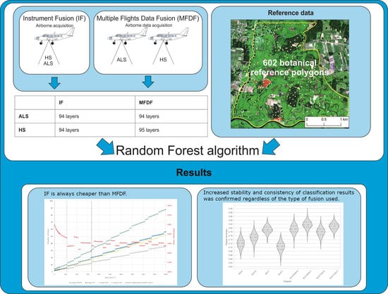
4.2. IF vs. MFDF Instrument Fusion vs. Multiple Flights Data Fusion

To our knowledge, until now, there have been no studies comparing results of classifications carried out using real data collected through MFDF or IF. Theoretical and experimental considerations suggest that IF data would yield higher accuracy [15,21], focusing on the analysis of the influence of the data’s geometric accuracy. Considering the conclusions from previous research, this study achieved subpixel co-registration accuracy of all integrated data in both MFDF and IF approaches. The results shown in Figure 2 and Table 6 indicate the resulting increase of Kappa accuracies of the classification on three non-forest Natura 2000 habitats when using MFDF or IF compared to using SS data (Table 6). Employing data fusion results in increased Kappa values regardless of the fusion type (IF, MFDF). Similar findings were observed by other researchers who used IF to increase the accuracy of tree species identification [49], or invasive species classification [50] compared to SS data classification.
MFDF data fusion of ALS17HS15 data with inherently low SS accuracy yielded an average increase in Kappa values by 0.10. As a comparison, the lowest increase in Kappa values, an average of 0.07, was recorded for MFDF data fusion of ALS15HS17 with inherently high SS accuracy (Figure 2, Table 6). Similar trends were observed in the classification of tree species, achieving an average Kappa value increase of 0.21 by fusing data with varying accuracy (0.53 using ALS, 0.73 using HS and 0.74 using IF) [49]. The range of output classifications of non-forest Natura 2000 habitats using data fusion remained in the Kappa 0.04 range (Table 6). This confirms the increased stability of output classification results, regardless of the type of data fusion used and the information load of SS data for which Kappa stayed within the 0.09 range (Table 6).
The two top classification results (ALS15HS17 and ALS17HS17) differed by only 0.01, leaning to the advantage of MFDF over IF (Figure 2, Table 6). It should be noted, however, that MFDF fusion results (ALS15HS17) were obtained by combining highly accurate SS data created artificially by combining data from different years. Conversely, when MFDF fusion was executed on SS data from the same year (ALS15HS15), the resulting classification accuracy was below that of IF data fusion (ALS17HS17). At the same time, the ALS17HS17 data fusion yielded the highest increase in Kappa value of 0.16, compared to ALS17, by fusing SS data with significantly differing accuracy (Figure 2, Table 6). Without complete knowledge of the influence of factors determined by the conditions of aerial data collection on SS data relevance, the application of data fusion minimizes the risk of not yielding consistent results that meet the expected classification accuracy levels. This finding is inconsistent with the findings of researchers studying savanna ecosystems [49], who argue that based on obtained tree classification results, the “classification with HS achieved results close enough to a fused classification approach and as such negated the need to include costly LiDAR”. Such conclusions were drawn with only one repetition and not considering the influence of data fusion on output stability, and without ensuring the application of comparable HS and ALS data parameters.
The differences in classification between MFDF and IF were expected to result from data incoherence ensuing from changes occurring in the study area between individual data collection runs using MFDF. The dynamic environment of a river valley can see changes in natural habitats occur in a matter of days due to varying water conditions or agricultural use, or in a matter of 1–2 years due to growth of expansive species or differing patterns of land use [51]. The 0.01 difference in Kappa values between the best classification results using MFDF (ALS15HS17) and IF (ALS17HS17) may lead to a conclusion that data coherence pursuant to simultaneous data collection (IF) is of lesser importance, compared to the data relevance of MFDF. However, we need to remember that during preparation of the set of reference polygons using MFDF, samples exhibiting real change that occurred between 2015 and 2017 were eliminated. The resulting number of reference polygons dropped by 17% (Table 4); this mitigated any inconsistency in training and validation datasets at the stage of machine learning. However, the data inconsistency problem remained unresolved at the stage of extrapolating the model onto the map—outside the reference polygon areas. Considering the above and Kappa differences of 0.01 between the two top classification results using MFDF (ALS15HS17) and IF (ALS17HS17), the use of IF classification seems to prevail over MFDF in terms of effectiveness.
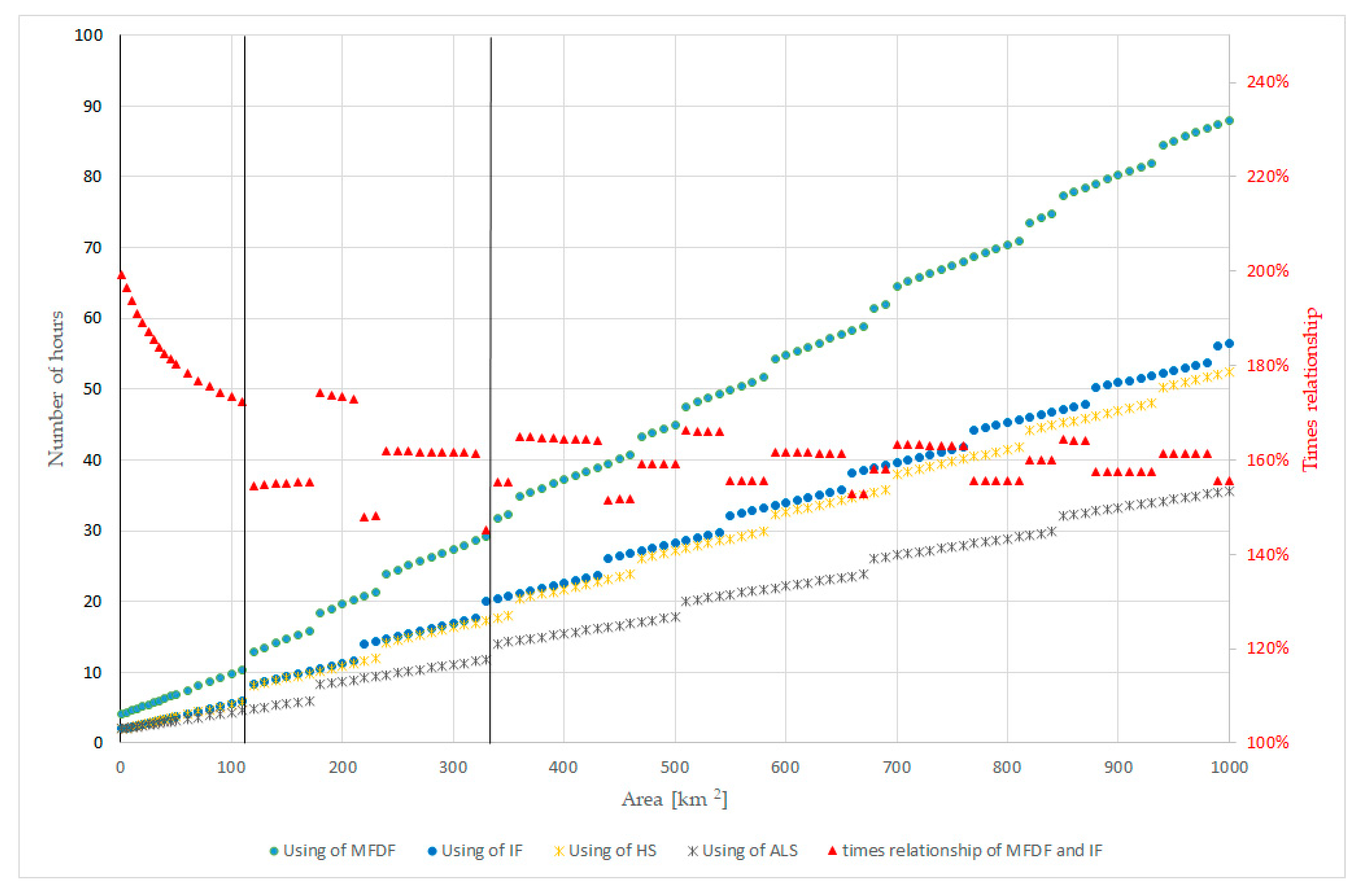
The most natural and simple solution for the application of data fusion is to combine data collected in MFDF [52,53,54]. This kind of data fusion does not require the use of non-standard technical solutions. There is evidence indicating that this method of data collection is prone to the risk of geometric incoherence [21] of terrain coverage of the data being fused. As a natural consequence, it became necessary to identify a solution to mitigate this risk. The solution was the application of IF, which yielded higher Kappa accuracy. In addition, the cost-effectiveness analysis of data fusion favors IF over MFDF. According to the assumptions used in similar analyses, the costs of collecting aerial data for similar purposes have been compared [55]. It was assumed that the data collection flights account for the highest cost in the remote sensing analysis budget [56] and the costs relating to processing and analysis of aerial remote sensing data are the same for MFDF and IF. As a consequence, the comparison of data collection flight time using MFDF and IF illustrates the benefit of using the IF method. MFDF data collection time equals the sum of total time collecting HS and ALS data, while the same data collected using IF equals to 106% of the HS data collection time. The time required to collect the data depends on the size of the studied area. Considering these two variables, the greater the area of data collection, the greater the difference between the time necessary for data collection using both data fusion methods. The greatest difference—of nearly 200%—in efficiency between IF and MFDF occurs when the collection area allows simultaneous data collection using IF during a single flight. For sensors used in the study, this was a study area of 110 km2. For areas larger than 330 km2, the difference in effectiveness between MFDF and IF stabilizes, oscillating (+/- 10%) at around 160%. The efficiency thresholds connected with the studied area size depend on attainable airspeed, single flight time, and selection of sensors with comparable efficiency at the given flight parameters. This is confirmed by similar findings [56] comparing the effectiveness of UAV airborne and orbital platforms. This is of particular importance, because aerial remote sensing data analysis using HS and ALS data fusion is most commonly conducted for areas up to 100 km2 e.g., [18,38] rarely reaching an area of 300 km2 e.g., [57,58].
The shorter time required for IF aerial data collection reduces the risk of data collection interruption caused by atmospheric conditions or another force majeure. Furthermore, IF ensures data consistency in terms of changes of the studied object over time. This is particularly important for areas undergoing dynamic changes in vegetation even within days (due to agricultural use or floods).

4.3. Further Development of Instrument Fusion

The development of IF is determined by the availability of applicable remote sensing equipment. During the last decade, several IF platforms have been engineered to integrate existing LiDAR and hyperspectral sensors, such as the CAO platform described by Asner et al. [14], the AOP platform by Kampe et al. [59] and the HabitARS platform built by the authors of this study. Cook et al. [15] created the G-LiHT platform combining LiDAR, hyperspectral and thermal scanners. It is to be expected that more and more sensors will be integrated and their working parameters can be optimized in a more consistent way, thus allowing data collection with even greater spatial resolution and data collection efficiency.

5. Conclusions

Based on these findings, it is impossible to determine which sensor—HS or ALS—used independently leads to higher classification accuracy of non-forest vegetation. Using only one data source is risky in terms of yielding consistent expected classification accuracy. The information relevance of ALS or HS data becomes known only during the data analysis stage. The findings show ALS sensors to be 40% more efficient than HS, with the difference depending on data parameters and employed sensors. ALS prevails over HS as an active sensor able to operate irrespective of lighting conditions.
The study shows the application of data fusion increases classification accuracy regardless of the type of data fusion (IF, MFDF). Findings also confirm the increase in stability and consistency of classification results irrespective of the type of data fusion and the degree of data relevance variation of collected SS data. Data collection using MFDF or IF does not determine the relevance level of ALS or HS data. Without complete understanding of the influence of factors determined by the conditions of aerial data collection on SS data relevance, the application of data fusion does minimize the risk of not yielding consistent and sufficiently accurate classification results. In comparison, IF yielded more accurate results than MFDF.
Data collection costs are 6% higher with the application of IF and 69% higher for MFDF, compared to the cost of SS data collection using HS. IF is always cheaper than MFDF. The difference in the efficiency of both methods becomes greater when the area of aerial data collection is larger. The highest efficiency of IF is for areas smaller than 110 km2, when data collection requires a single flight only. The efficiency of data collection using data fusion depends on the speed and duration of a single flight and the application of sensors with similar operating parameters to the given flight parameters. IF eliminates the risk of mutual data incoherence of HS and ALS data, in terms of geometry, terrain coverage and atmospheric conditions due to different collection times. The individual and specific need to combine data collection sensors for remote sensing studies ensures that the application of IF in the aerial data collection market is determined by the availability of existing technological solutions.

Author Contributions

Conceptualization—Ł.S., J.N. and D.K.; Investigation—Ł.S., J.N. and D.K.; Methodology—Ł.S., J.N. and D.K.; Project administration, Ł.S; Resources—Ł.S., D.K. and H.P.; Experiment design and execution—Ł.S., D.K., J.N. and A.K.; Supervision—D.K.; Validation—Ł.S., J.N. and D.K.; Visualization—Ł.S., J.N. and A.K.; Writing—original draft, Ł.S., J.N. and D.K.; Writing—review & editing, D.K.

Funding

The IF work and construction of the HabitARS multisensor platform was co-financed by the Polish National Centre for Research and Development (NCBR) and MGGP Aero under the programme, “Natural Environment, Agriculture and Forestry” BIOSTRATEG II: The innovative approach supporting monitoring of non-forest Natura 2000 habitats, using remote sensing methods (HabitARS); project number DZP/BIOSTRATEG-II/390/2015. The Consortium Leader is MGGP Aero. The project partners include University of Lodz, University of Warsaw, Warsaw University of Life Sciences, Institute of Technology and Life Sciences, University of Silesia in Katowice, and Warsaw University of Technology.

Acknowledgments

The MFDF work was made possible through a commercial contract for the “Collection of comprehensive remote sensing data and their analysis for the area of the Lower Biebrza Valley Basin,” commissioned in the years 2015–2016 by the Biebrzański National Park and financed by the National Fund for Environmental Protection and Water Management within the framework of the project “Assessment of the state of natural resources and emerging threats in the Lower Basin of Biebrza Valley”. The authors thank the reviewers and William Oxford for the helpful comments.

Conflicts of Interest

The authors declare no conflict of interest. The founding sponsors had no role in the design of the study; in the collection, analyses or interpretation of data; in the writing of the manuscript and in the decision to publish the results.

References

  1. Wald, L. Some terms of reference in data fusion. IEEE Trans. Geosci. Remote Sens. 1999, 37, 1190–1193. [Google Scholar] [CrossRef] [Green Version]
  2. Ruser, H.; León, F.P. Informationsfusion—Eine Übersicht (Information Fusion—An Overview). Tech. Mess. 2007, 74, 93–102. [Google Scholar] [CrossRef]
  3. Hackett, J.K.; Shah, M. Multi-sensor fusion: A perspective. In Proceedings of the IEEE International Conference: Robotics and Automation, Cincinnati, OH, USA, 13–18 May 1990. [Google Scholar]
  4. Stenzel, S.; Feilhauer, H.; Mack, B.; Metz, A.; Schmidtlein, S. Remote sensing of scattered Natura 2000 habitats using a one-class classifier. Int. J. Appl. Earth Obs. Geoinf. 2014, 33, 211–217. [Google Scholar] [CrossRef]
  5. Mücher, C.A.; Kooistra, L.; Vermeulen, M.; Borre, J.V.; Haest, B.; Haveman, R. Quantifying structure of Natura 2000 heathland habitats using spectral mixture analysis and segmentation techniques on hyperspectral imagery. Ecol. Indic. 2013, 33, 71–81. [Google Scholar] [CrossRef]
  6. Schmidt, J.; Fassnacht, F.E.; Neff, C.; Lausch, A.; Kleinschmit, B.; Förster, M.; Schmidtlein, S. Adapting a Natura 2000 field guideline for a remote sensing-based assessment of heathland conservation status. Int. J. Appl. Earth Obs. Geoinf. 2017, 60, 61–71. [Google Scholar] [CrossRef]
  7. Feilhauer, H.; Dahlke, C.; Doktor, D.; Lausch, A.; Schmidtlein, S.; Schulz, G.; Stenzel, S. Mapping the local variability of Natura 2000 habitats with remote sensing. Appl. Veg. Sci. 2014, 17, 765–779. [Google Scholar] [CrossRef]
  8. Hladik, C.; Schalles, J.; Alber, M. Salt marsh elevation and habitat mapping using hyperspectral and LIDAR data. Remote Sens. Environ. 2013, 139, 318–330. [Google Scholar] [CrossRef]
  9. Onojeghuo, A.O.; Onojeghuo, A.R. Object-based habitat mapping using very high spatial resolution multispectral and hyperspectral imagery with LiDAR data. Int. J. Appl. Earth Obs. Geoinf. 2017, 59, 79–91. [Google Scholar] [CrossRef]
  10. Kopeć, D.; Michalska-Hejduk, D.; Sławik, Ł.; Berezowski, T.; Borowski, M.; Rosadziński, S.; Chormański, J. Application of multisensoral remote sensing data in the mapping of alkaline fens Natura 2000 habitat. Ecol. Indic. 2016, 70, 196–208. [Google Scholar] [CrossRef]
  11. Simone, G.; Farina, A.; Morabito, F.C.; Serpico, S.; Bruzzone, L. Image fusion techniques for remote sensing applications. Inf. Fusion 2002, 3, 3–15. [Google Scholar] [CrossRef] [Green Version]
  12. Piiroinen, R.; Heiskanen, J.; Maeda, E.; Hurskainen, P.; Hietanen, J.; Pellikka, P. Mapping Land Cover in the Taita Hills, Se Kenya, Using Airborne Laser Scanning and Imaging Spectroscopy Data Fusion. ISPRS Int. Arch. Photogramm. Remote Sens. Spat. Inf. Sci. 2015, 40, 1277–1282. [Google Scholar] [CrossRef]
  13. Alonzo, M.; Bookhagen, B.; Roberts, D.A. Urban tree species mapping using hyperspectral and lidar data fusion. Remote Sens. Environ. 2014, 148, 70–83. [Google Scholar] [CrossRef]
  14. Asner, G.P.; Knapp, D.E.; Kennedy-Bowdoin, T.; Jones, M.O.; Martin, R.E.; Boardman, J.; Hughes, R.F. Invasive species detection in Hawaiian rainforests using airborne imaging spectroscopy and LiDAR. Remote Sens. Environ. 2008, 112, 1942–1955. [Google Scholar] [CrossRef]
  15. Cook, B.D.; Corp, L.A.; Nelson, R.F.; Middleton, E.M.; Morton, D.C.; McCorkel, J.T.; Masek, J.G.; Ranson, K.J.; Ly, V.; Montesano, P.M. NASA Goddard’s LiDAR, Hyperspectral and Thermal (G-LiHT) Airborne Imager. Remote Sens. 2013, 5, 4045–4066. [Google Scholar] [CrossRef] [Green Version]
  16. Pang, Y.; Li, Z.; Ju, H.; Lu, H.; Jia, W.; Si, L.; Guo, Y.; Liu, Q.; Xie, B.; Tan, B.; et al. LiCHy: The CAF’s LiDAR, CCD and Hyperspectral Integrated Airborne Observation System. Remote Sens. 2016, 8, 398. [Google Scholar] [CrossRef]
  17. García, M.; Riaño, D.; Chuvieco, E.; Salas, J.; Danson, F.M. Multispectral and LiDAR data fusion for fuel type mapping using Support Vector Machine and decision rules. Remote Sens. Environ. 2011, 115, 1369–1379. [Google Scholar] [CrossRef]
  18. Onojeghuo, A.O.; Blackburn, G.A. Optimising the use of hyperspectral and LiDAR data for mapping reedbed habitats. Remote Sens. Environ. 2011, 115, 2025–2034. [Google Scholar] [CrossRef]
  19. Jones, T.G.; Coops, N.C.; Sharma, T. Assessing the utility of airborne hyperspectral and LiDAR data for species distribution mapping in the coastal Pacific Northwest, Canada. Remote Sens. Environ. 2010, 114, 2841–2852. [Google Scholar] [CrossRef]
  20. Colgan, M.S.; Baldeck, C.A.; Feret, J.-B.; Asner, G.P. Mapping Savanna Tree Species at Ecosystem Scales Using Support Vector Machine Classification and BRDF Correction on Airborne Hyperspectral and LiDAR Data. Remote Sens. 2012, 4, 3462–3480. [Google Scholar] [CrossRef] [Green Version]
  21. Asner, G.P.; Knapp, D.E.; Boardman, J.; Green, R.O.; Kennedy-Bowdoin, T.; Eastwood, M.; Martin, R.E.; Anderson, C.; Field, C.B. Carnegie Airborne Observatory-2: Increasing science data dimensionality via high-fidelity multi-sensor fusion. Remote Sens. Environ. 2012, 124, 454–465. [Google Scholar] [CrossRef]
  22. Torabzadeh, H.; Morsdorf, F.; Schaepman, M.E. Fusion of imaging spectroscopy and airborne laser scanning data for characterization of forest ecosystems—A review. ISPRS J. Photogramm. Remote Sens. 2014, 97, 25–35. [Google Scholar] [CrossRef]
  23. Brennan, R.L.; Prediger, D.J. Coefficient Kappa: Some Uses, Misuses, and Alternatives. Educ. Psychol. Meas. 1981, 41, 687–699. [Google Scholar] [CrossRef]
  24. Borre, J.V.; Paelinckx, D.; Mücher, C.A.; Kooistra, L.; Haest, B.; De Blust, G.; Schmidt, A.M. Integrating remote sensing in Natura 2000 habitat monitoring: Prospects on the way forward. J. Nat. Conserv. 2011, 19, 116–125. [Google Scholar] [CrossRef]
  25. HySpex RAD. Available online: https://www.hyspex.no/ (accessed on 1 March 2018).
  26. PARGE ReSe Applications. Available online: https://www.rese-apps.com/software/parge/index.html (accessed on 1 March 2018).
  27. ATCOR4 Manual. ReSe Applications. Available online: https://www.rese-apps.com/pdf/atcor4_manual.pdf (accessed on 1 March 2018).
  28. RiProcess Data Sheet for RIEGL Scan Data. Available online: http://www.riegl.com/uploads/tx_pxpriegldownloads/11_Datasheet_RiProcess_2016-09-16_01.pdf (accessed on 16 September 2016).
  29. RiAnalyze Data Sheet for Automated Resolution of Range Ambiguities. Available online: http://www.riegl.com/uploads/tx_pxpriegldownloads/11_DataSheet_RiMTA-ALS_2015-08-24_03.pdf (accessed on 24 August 2015).
  30. TerraSolid Terrascan User Guide. Available online: http://www.terrasolid.com/guides/tscan/index.html (accessed on 20 July 2018).
  31. ENVI API Programming Guide. Harris Geospatial Solutions Documentation Center. Available online: http://www.harrisgeospatial.com/docs/ProgrammingGuideIntroduction.html (accessed on 21 December 2017).
  32. OPALS Reference Documentation. Department of Geodesy and Geoinformation—Technische Universität Wien. Available online: https://geo.tuwien.ac.at/opals/html/ref_index.html (accessed on 23 April 2018).
  33. SAGA GIS Documentation. SAGA User Group Association. Available online: https://sourceforge.net/p/saga-gis/wiki/General%20Documentation/ (accessed on 28 February 2019).
  34. Breiman, L. Random forest. Mach. Learn. 2001, 45, 1–33. [Google Scholar] [CrossRef]
  35. Chutia, D.; Bhattacharyya, D.K.; Sarma, K.K.; Kalita, R.; Sudhakar, S. Hyperspectral Remote Sensing Classifications: A Perspective Survey. Trans. GIS 2016, 20, 463–490. [Google Scholar] [CrossRef]
  36. Cutler, D.R.; Edwards, T.C.; Beard, K.H.; Cutler, A.; Hess, K.T.; Gibson, J.; Lawler, J.J. Random forests for classification in ecology. Ecology 2007, 88, 2783–2792. [Google Scholar] [CrossRef]
  37. Rodriguez-Galiano, V.F.; Ghimire, B.; Rogan, J.; Olmo, M.C.; Rigol-Sanchez, J.P. An assessment of the effectiveness of a random forest classifier for land-cover classification. ISPRS J. Photogramm. Remote Sens. 2012, 67, 93–104. [Google Scholar] [CrossRef]
  38. Pelletier, C.; Valero, S.; Inglada, J.; Champion, N.; Sicre, C.M.; Dedieu, G. Effect of Training Class Label Noise on Classification Performances for Land Cover Mapping with Satellite Image Time Series. Remote Sens. 2017, 9, 173. [Google Scholar] [CrossRef]
  39. Vegetation Classification Studio Software, Version 2.13/hb. Available online: http://www.definity.pl/vcs (accessed on 5 March 2019).
  40. STATISTICA (Data Analysis Software System), Version 12. Available online: www.statsoft.com (accessed on 1 March 2018).
  41. Zlinszky, A.; Deák, B.; Kania, A.; Schroiff, A.; Pfeifer, N. Biodiversity mapping via natura 2000 conservation status and ebv assessment using airborne laser scanning in alkali grasslands. ISPRS Int. Arch. Photogramm. Remote Sens. Spat. Inf. Sci. 2016, 41, 1293–1299. [Google Scholar] [CrossRef]
  42. Zlinszky, A.; Schroiff, A.; Kania, A.; Deák, B.; Mücke, W.; Vári, Á.; Székely, B.; Pfeifer, N. Categorizing grassland vegetation with full-waveform airborne laser scanning: A feasibility study for detecting natura 2000 habitat types. Remote Sens. 2014, 6, 8056–8087. [Google Scholar] [CrossRef]
  43. Haest, B.; Vanden Borre, J.; Spanhove, T.; Thoonen, G.; Delalieux, S.; Kooistra, L.; Mücher, C.; Paelinckx, D.; Scheunders, P.; Kempeneers, P. Habitat Mapping and Quality Assessment of NATURA 2000 Heathland Using Airborne Imaging Spectroscopy. Remote Sens. 2017, 9, 266. [Google Scholar] [CrossRef]
  44. Neumann, C.; Weiss, G.; Schmidtlein, S.; Itzerott, S.; Lausch, A.; Doktor, D.; Brell, M. Gradient-Based Assessment of Habitat Quality for Spectral Ecosystem Monitoring. Remote Sens. 2015, 7, 2871–2898. [Google Scholar] [CrossRef] [Green Version]
  45. Elmasry, G.; Kamruzzaman, M.; Sun, D.-W.; Allen, P. Principles and Applications of Hyperspectral Imaging in Quality Evaluation of Agro-Food Products: A Review. Crit. Rev. Sci. Nutr. 2012, 52, 999–1023. [Google Scholar] [CrossRef] [PubMed]
  46. Baltsavias, E.P. A comparison between photogrammetry and laser scanning. ISPRS J. Photogramm. Remote Sens. 1999, 54, 83–94. [Google Scholar] [CrossRef]
  47. Shaw, G.A.; Burke, H.K. Spectral Imaging for Remote Sensing. Lincoln Lab. J. 2003, 14, 3–28. [Google Scholar] [CrossRef]
  48. Zhang, J.; Erway, J.; Hu, X.; Zhang, Q.; Plemmons, R. Randomized SVD Methods in Hyperspectral Imaging. J. Electr. Comput. Eng. 2012, 2012, 1–15. [Google Scholar] [CrossRef] [Green Version]
  49. Sarrazin, M.J.D.; van Aardt, J.A.N.; Asner, G.P.; Mcglinchy, J.; Messinger, D.W.; Wu, J. Fusing small-footprint waveform LiDAR and hyperspectral data for canopy-level species classification and herbaceous biomass modeling in savanna ecosystems. Can. J. Remote Sens. 2011, 37, 653–665. [Google Scholar] [CrossRef]
  50. Marcinkowska-Ochtyra, A.; Jarocińska, A.; Bzdęga, K.; Tokarska-Guzik, B. Classification of Expansive Grassland Species in Different Growth Stages Based on Hyperspectral and LiDAR Data. Remote Sens. 2019, 10, 2019. [Google Scholar] [CrossRef]
  51. Adam, E.; Mutanga, O.; Rugege, D. Multispectral and hyperspectral remote sensing for identification and mapping of wetland vegetation: A review. Wetl. Ecol. Manag. 2010, 18, 281–296. [Google Scholar] [CrossRef]
  52. Grime, S.; Durrant-Whyte, H. Data fusion in decentralized sensor networks. Control Eng. Pract. 1994, 2, 849–863. [Google Scholar] [CrossRef]
  53. Buddenbaum, H.; Seeling, S.; Hill, J. Fusion of full-waveform lidar and imaging spectroscopy remote sensing data for the characterization of forest stands. Int. J. Remote Sens. 2013, 34, 4511–4524. [Google Scholar] [CrossRef]
  54. Kaasalainen, S.; Pyysalo, U.; Krooks, A.; Vain, A.; Kukko, A.; Hyyppä, J.; Kaasalainen, M. Absolute Radiometric Calibration of ALS Intensity Data: Effects on Accuracy and Target Classification. Sensors 2011, 11, 10586–10602. [Google Scholar] [CrossRef] [PubMed] [Green Version]
  55. Watkins, T.H. The Economics of Remote Sensing. J. Am. Soc. Photogramm. 1978, 44, 1167–1172. [Google Scholar]
  56. Matese, A.; Toscano, P.; Di Gennaro, S.F.; Genesio, L.; Vaccari, F.P.; Primicerio, J.; Belli, C.; Zaldei, A.; Bianconi, R.; Gioli, B. Intercomparison of UAV, Aircraft and Satellite Remote Sensing Platforms for Precision Viticulture. Remote Sens. 2015, 7, 2971–2990. [Google Scholar] [CrossRef] [Green Version]
  57. Anderson, J.E.; Plourde, L.C.; Martin, M.E.; Braswell, B.H.; Smith, M.-L.; Dubayah, R.O.; Hofton, M.A.; Blair, J.B. Integrating waveform lidar with hyperspectral imagery for inventory of a northern temperate forest. Remote Sens. Environ. 2008, 112, 1856–1870. [Google Scholar] [CrossRef]
  58. Mitchell, J.J.; Shrestha, R.; Spaete, L.P.; Glenn, N.F. Combining airborne hyperspectral and LiDAR data across local sites for upscaling shrubland structural information: Lessons for HyspIRI. Remote Sens. Environ. 2015, 167, 98–110. [Google Scholar] [CrossRef]
  59. Kampe, T.U.; Johnson, B.R.; Kuester, M.A.; Keller, M. NEON: The first continental-scale ecological observatory with airborne remote sensing of vegetation canopy biochemistry and structure. J. Appl. Remote Sens. 2010, 4, 043510. [Google Scholar] [CrossRef]
Figure 1. Study Area, Lower Biebrza, Poland.
Remotesensing 11 00970 g001
Figure 2. Violin plots illustrating averages, quartiles, and shape of distributions of Kappa accuracy values for eight classification scenarios using different raster sets of input data. Kappa accuracy values were calculated from the 1000 repetitions of the classification in each scenario, with varying randomized sets of training and validation sampled with 50%/50% proportion. All scenarios’ results differ statistically (one-way ANOVA with Tukey post-hoc test, p < 0.05). Abbreviations: HS—Hyperspectral; ALS—Aerial Laser Scanning; 15—year 2015; 17—year 2017.
Remotesensing 11 00970 g002
Figure 3. Number of hours using MFDF, IF, hyperspectral scanners, LiDAR scanner, and the time relationship of MFDF against IF data collection for flyover surface areas ranging from 1 to 1000 square kilometers. Abbreviations: HS—Hyperspectral images; ALS—Airborne Laser Scanning; MFDF—Multiple Flights Data Fusion; IF—Instrument Fusion.
Remotesensing 11 00970 g003
Table 1. Multiple flights data fusion—fusion of data collected with different sensors in multiple flights. Abbreviations: HS—Hyperspectral; ALS—Aerial Laser Scanning; VNIR—Visual-Near Infrared; SWIR—Short Wave Infrared; GSD—Ground Sampling Distance; AGL—Above Ground Level.
Data TypeSensor TypeData ParametersFlight Line Overlap [%]Swath Width [m]AircraftFlight Level [m] and Airspeed [m/s]Date of Flight
ALS point cloudRiegl LiteMapperDensity 4 [pts.m2] × 2 = 8 [pts./m2]60577Vulcan Air P68 Observer2500 AGL, 51.52 July 2015
HS imagesHySpex VNIR-1800 0.4–0.9 µmGSD 1 [m]30874Cessna 402B1450 AGL, 64.53 July 2015
HS imagesHySpex SWIR-384 0.9–2.5 µmGSD 2 [m]25813
Table 2. Fusion of data collected with different sensors in a single flight, using the HabitARS platform. Abbreviations: HS—Hyperspectral; ALS—Aerial Laser Scanning; VNIR—Visual-Near Infrared; SWIR—Short Wave Infrared; RGB—Red Green Blue; GSD—Ground Sampling Distance; AGL—Above Ground Level.
Data TypeSensor TypeData ParametersFlight Line Overlap [%]Swath Width [m]AircraftsFlight Level [m] and Airspeed [m/s]Date of Flight
ALS point cloudRiegl LiteMapperdensity 3.5 [pts./m2] × 2 = 7 [pts./m2]67843Cessna CT206H 730 AGL, 59.227 June 2017 and 1 July 2017
HS imagesHySpex VNIR-1800 0.4-0.9 µmGDS 0.49 [m]35440
HS imagesHySpex SWIR-384 0.9-2.5 µmGDS 1.07 [m]30410
RGB imagesRGB Digital CameraGDS 0.1 [m]60/60710
Table 3. Number of products broken down by source and data collection method. Abbreviations: HS—Hyperspectral; ALS—Aerial Laser Scanning.
Data SourceAcquisition Year (Method)2017 (IF)
2015 (MFDF)
ALS94 layers – ALS1594 layers – ALS17
HS95 layers – HS1595 layers – HS17
Table 4. Number of reference polygons before and after visual verification according to type of Natura 2000 habitats and backgrounds.
Name of the Natura 2000 Habitat TypeNatura 2000 Habitat CodeNumber of Reference Polygons
Before VerificationAfter Verification against Shadows and Mowed in 2015 and 2017
Xeric sand calcareous grasslands612011292
Alluvial meadows of river valleys of the Cnidion dubii6440202161
Species-rich Nardus grasslands62301313
Background9999380336
Sum 707602
Table 5. Sets of raster data used in individual classification scenarios. Abbreviations: HS—Hyperspectral images; ALS—Airborne Laser Scanning, SS—Single Sensor; MFDF—Multiple Flights Data Fusion; IF—Instrument Fusion; 15—year 2015; 17—year 2017.
Scenario NameHS15ALS15HS17ALS17ALS15HS15ALS15HS17ALS17HS15ALS17HS17
Fusion methodSSSSSSSSMFDFMFDFMFDFIF
HS2015
ALS2015
HS2017
ALS2017
Table 6. Accuracy gains between average single sensor Kappa accuracy and data fusion Kappa accuracy. Subtracted values are the average of 1000 classifications with randomly varying training and validation sets in 50%/50% proportion. Abbreviations: HS—Hyperspectral; ALS—Aerial Laser Scanning.
Type of FusionMultiple Flights Data FusionInstrument Fusion
Data fusion Kappa accuracyALS15HS15ALS17HS15ALS15HS17ALS17HS17
0.790.780.820.81
Single sensor Kappa accuracyALS15 0.75HS15 0.72ALS17 0.70HS15 0.72ALS15 0.75HS17 0.79ALS17 0.70HS17 0.79
Increase of Kappa accuracy after data fusion in comparison to Single sensor classification5.3%9.7%11.4%8.3%9.3%3.8%15.7%2.5%
Average increase of Kappa accuracy after data fusion in comparison to Single sensor classificationALS15HS15 7.5%ALS17HS15 9.7%ALS15HS17 6.5%ALS17HS17 9.1%
Table 7. Theoretical MFDF flight parameters equal to the parameters of IF data. Abbreviations: HS—Hyperspectral; ALS—Aerial Laser Scanning; VNIR—Visual-Near Infrared; SWIR—Short Wave Infrared; GSD—Ground Sampling Distance; AGL—Above Ground Level.
Data TypeSensor TypeData ParametersFlight Line Overlap [%]Swath Width [m]AircraftFlight Level [m] Airspeed [m/s]
ALS point cloudRiegl LiteMapperdensity 7 [pts./m2]25577Cessna CT206H500 AGL61,8
HS imagesHySpex VNIR-1800 0.4–0.9 µmGSD 0.49 [m]35440730 AGL66,9
HS imagesHySpex SWIR-384 0.9–2.5 µmGSD 1.07 [m]30410

